
Abstract
Protein interaction networks provide useful information to assess impacts of disease on cell functions. Statistical clustering methods applied to these networks can reveal impacts on particular functional groups of proteins. In addition, clustering methods can identify subsets of proteins that require additional study to provide updated information regarding their position within an interaction network, and hence increase our understanding of their relationships with other proteins in the network. These ideas are illustrated here by considering the impacts of sickle cell disease on the human erythrocyte interaction network. Statistical cluster analyses are performed based on a measure of similarity for nodes within a network called the Generalized Topological Overlap Measure. These analyses identify clusters of proteins that are similar in terms of shared interaction partners. Identification of clusters that contain proteins whose relative abundances have been significantly altered in sickle cell patients provides specific information about the impact of these proteins on erythrocyte functions.
Introduction
The human erythrocyte protein interactome (HEPI) is a complex network consisting of a set of nodes and edges connecting the nodes. The nodes are comprised of the set of all proteins present in erythrocytes. This set is referred to as the erythrocyte proteome. The edges of this network are the interactions between proteins in the proteome. The HEPI is partially known (1). We can obtain estimates of this interactome that are constructed from proteomic databases, but these estimates are dynamic. Additional nodes (proteins) may be added as more experiments are performed, and some nodes may be removed as differences in protein naming conventions are resolved. More edges (interactions) may be added and some edges may be removed (false positives) as experiments are performed to test some inferred interactions. Considerable effort is required to collect the results of research conducted globally to identify protein interactions. The Unified Human Interactome, described in (2), and STRING, described in (3), are examples of web-based databases for protein interactions that have been made available to the research community.
An example of the potential role these efforts can play in the study of systems biology of disease mechanisms is discussed in Goodman, et al. (1). This paper describes how proteomics can aid in the understanding of sickle cell disease (SCD). SCD is the result of a point mutation of the β-globin gene on chromosome 11. In homozygous sickle cell patients, thymine replaces adenine at one point within this gene, and the miscoding caused by this mutation results in a single amino acid substitution, valine for glutamic acid, in a component of hemoglobin. The discovery of this modified form of hemoglobin as the underlying cause of SCD in 1956 represented the first time the molecular basis of a genetic disorder was identified. Although the genetic basis for SCD has been known for more than fifty years, there is much about this disease that remains to be discovered. In particular, even though the same genetic mutation is responsible for the presence of SCD in patients, there is a wide range in severity of its symptoms. For example, acute pain associated with vaso-occlusive events or acute chest syndrome vary greatly among SCD patients, and those with high lifetime rates of these events exhibit higher mortality. Therefore, other processes must contribute to the differential severity of SCD symptoms. A greater understanding of the systems biology associated with this disease should greatly enhance the development of effective therapies that address the causes of SCD disease severity, not just its external symptoms.
To aid in our understanding of the impact sickle cell disease (SCD) has on the HEPI network, we examine clustering tools that place proteins into groups that are similar according to criteria defined by those tools. A number of studies (4–7) have shown that proteins with high overlap of the number of shared interactions are more likely to belong to the same functional class. Therefore, use of this criterion for clustering has the potential to expose functional group membership of proteins from protein interaction databases. If a protein that is not a member of a particular functional group but has links with a small proportion of that group’s proteins, then that protein would not be considered close to the group as measured by GTOM. Likewise, if a protein links with only a few members of a functional group but, due to lack of supporting research, this protein is a member of that group, then the protein would not be close to the group under the GTOM criterion. However, if studies indicate that the abundance of this protein is significantly impacted by the presence or severity of a disease, then it would be warranted to study this protein’s possible interactions with proteins in clusters to which it is has at least one link. Although application of these clustering tools to SCD is described here, these tools could be applied to other diseases, other families of proteins, and to other species.
Methods
Since protein interaction databases are frequently updated, an estimate of the HEPI was obtained by entering the proteome obtained from (1) into the Unified Human Interactome (UniHI) (2). Protein interactions with negative Spearman correlations were deleted. This updated interactome is shown in Supplemental Figure S1.
Clustering Based on the Generalized Topological Overlap Measure.
Recently a new measure of similarity between nodes in a network has been proposed called the Generalized Topological Overlap Measure (GTOM) (8). GTOM for proteins A and B is based on the intersection of the sets of proteins that are within an m-step neighborhood of A and B, respectively, in the protein interaction network. That is, proteins A and B are 1-step apart if A and B interact and they are 2-steps apart if there is a third protein which interacts with A and B. Two proteins with a large number of shared interactions will have a high GTOM score, and so have high GTOM similarity. See (8) for a detailed description of this measure. Since GTOM is defined so that 0 ≤ GTOM(A,B) ≤ 1, then the matrix of GTOM similarities between all pairs of proteins in the network, T, can be transformed into a distance matrix, D, by D = 1 – T. Hierarchical or agglomerative clustering can be applied to this distance matrix to identify modules of similar proteins. Since the cut points used to define modules in clustering can be arbitrary, cut points are selected to satisfy some specified optimality criteria. Good criteria should make the resulting protein modules reasonably consistent with well-established functional classes when known.
Since GTOM is based on the numbers of proteins within a specified number of interaction links, the full interaction network is reduced initially to contain just those proteins that are part of the large, connected subgraph shown in Figure S1. This reduction results in a network of 340 proteins, all of which are connected by at least one interaction. To compare results, m = 1 and m = 2 are used to obtain two distance matrices using GTOM, denoted by GTOM1 and GTOM2, respectively. These distance matrices then can be used with a clustering algorithm to generate clusters of proteins such that two proteins within the same cluster are closer to (have more shared interactions with) each other than they are to proteins outside the cluster.
Two clustering algorithms are considered here, Agnes (agglomerative nesting), and Diana (divisive analysis). Agnes is similar to classical hierarchical clustering in that it begins with each protein in its own cluster and then performs a series of merges to reduce the number of clusters until there is just one cluster that contains all proteins. The Diana algorithm begins with all proteins in one cluster and then performs a series of splits until each protein is contained in its own cluster. The Agnes and Diana algorithms are described in detail in (9).
Number of Clusters.
With any clustering procedure there is some ambiguity regarding the choice of how many clusters of proteins should be defined. One approach to this problem suggested by (9) is to base the number of clusters on silhouette width. The silhouette width of a particular protein is defined as
where w denotes the average distance between this protein and all other proteins in the same cluster (within-cluster distance), and b denotes the minimum of the average distances between this protein and the proteins in each of the other clusters (between cluster distance). Proteins with high silhouette widths are relatively close to their cluster neighbors, and so this gives a measure of cluster homogeneity. Therefore, the number of clusters can be selected to maximize the average silhouette width (ASW) over all proteins. Note that this process can be applied to any clustering procedure.
An alternative criterion for selecting the number of clusters is the Mean Silhouette Split (MSS) (10). This criterion is defined as follows. Suppose the proteins have been split into N clusters. For cluster n, 1 ≤ n ≤ N, apply the clustering algorithm to the proteins in the cluster, and let SS n denote the maximum ASW among the sub-clusters of this cluster. The MSS for N clusters is defined to be
Note that MSS(N) is a measure of cluster heterogeneity. We select the number of clusters K to be the value of N that minimizes MSS(N),
An alternative criterion is to use the median instead of the mean,
The number of clusters is then
Results
Average Silhouette Width.
The ASW criterion was applied to the results of the clustering algorithms for GTOM1 and GTOM2 and gave the following cluster sizes.
GTOM1, Agnes: 161 GTOM1, Diana: 184 GTOM2, Agnes: 118 GTOM2, Diana: 140
An image of the distance matrix, called a heatmap, is an effective graphical tool to evaluate the results of a clustering algorithm. Small distances are displayed with darker red colors and large distances are displayed with lighter red colors. Color bars are shown in the margins to represent the clusters. Distance matrices with clearly defined clusters have heatmaps with low distances concentrated along diagonal blocks, and these blocks correspond to clusters defined by the algorithm. Heatmaps for the four cluster methods using the number of clusters selected by ASW are shown in Figures 1 and 2.
The heatmaps for GTOM2 (Fig. 2) show that this is not a useful distance measure for this protein interaction network since there is little concentration of small distances within diagonal blocks. The heatmaps for GTOM1 show good concentration along the diagonals for the larger clusters (Fig. 1). However, there are large numbers of single-protein clusters that are the result of the relatively high numbers of clusters selected by the ASW criterion.
Mean Silhouette Split.
Plots of MSS for GTOM1 and GTOM2 are shown in Figure 3. The optimal number of clusters based on Agnes clustering of GTOM1 was 64, and the optimal number based on Diana clustering of GTOM1 was 105. Both clustering methods have one large cluster that contains proteasome proteins, but it can be seen from their heatmaps (Figs. 4, 5) that Agnes has more moderately sized clusters with reasonable concentrations of small distances around diagonal blocks, whereas Diana clustering contains one large cluster with most of the remaining proteins located within small clusters.
Minimizing MSS using GTOM1 and Agnes gives 4 large clusters containing 51, 19, 18, 16 proteins, respectively. These proteins are listed in Tables 1a–d. The complete list of clusters is given in the Supplementary Material. Cluster 1 is dominated by proteasome proteins and proteins involved in ubiquitination. Cluster 2 contains proteins involved in purine synthesis. Cluster 3 contains binding proteins and antioxidants. Cluster 4 is dominated by chaperonins, but also includes some proteins involved in cell shape and motility.
The three largest clusters defined by minimum MSS using GTOM1 and Diana contain 41, 10, 9 proteins, respectively. These proteins are listed in Tables 2a–c. The complete list of clusters is given in the Supplementary Material in the online version. Cluster 1 is also dominated by proteosome proteins. However, unlike Agnes clustering results, the chaperonins are contained in four different clusters.
Also of interest are clusters that contain just a few proteins, especially if those proteins are not similar to each other according to known functions. These proteins are not sufficiently close to other proteins to be included in larger clusters, which implies that they have few interaction partners. This could arise because they have not been studied sufficiently to identify all of their interacting partners.
SCD-Altered Proteins.
We next consider proteins that are modified by sickle-cell disease. Determination of these proteins is described in (1). Table 3 lists these proteins and how their abundances were modified in SCD subjects relative to normal subjects. The column headed by Symbol gives the gene symbol of each protein; the column headed by Ent-GID gives the Entrez Gene ID of the corresponding proteins; the column headed by Altered indicates whether the relative protein abundance increased or decreased. An entry of Both indicates that some forms of the protein increased while others decreased. See (1) for details.
SCD-Altered Proteins in Agnes Clusters.
Clusters defined by Agnes for GTOM1 that contain SCD-altered proteins are given in Table 4 with the altered proteins underlined. Since multiple SCD-altered proteins appear in clusters 1 (proteasomes) and 4 (chaperonins), it is likely that the functioning of proteins in these clusters will be impacted by SCD. Note that
SCD-Altered Proteins in Diana Clusters.
Clusters defined by Diana for GTOM1 that contain SCD-altered proteins are given in Table 5 with the altered proteins underlined. As was the case with Agnes clusters, the proteasome cluster contains multiple SCD-altered proteins.
The clustering tools described here have revealed a number of erythrocyte proteins that require further study to increase our understanding of the impact of SCD on the HEPI. The following list of such proteins is based on Agnes clustering.
EHD1 and PRDX3 are SCD-impact proteins with no interactions with other erythrocyte proteins that satisfied the interaction selection criteria. EPB49 is in a small cluster with a spectrin protein, rather than with other erythrocyte membrane proteins, EPB41 and EPB42. This indicates that EPB49 should be studied further to determine if it shares interactions with other proteins in the cluster that contains EPB41 and EPB42. Many of the heat shock proteins had interactions with erythrocyte proteins that did not satisfy the initial selection criteria of a Spearman correlation greater than 0. The two that did, HSPA8 and HSPA1A, are in separate clusters. Since the Spearman correlation for an interaction measures coexpression of the corresponding genes, and since HSPA8 and HSPA1A are among the SCD-impacted proteins, further study of the interactions for this family of proteins is needed. STOM is in a small cluster with CALR, CANX, and SLC2A1. RAB8B is in a small cluster with RALA and RALBP1. ANK1 is in a small cluster with TTN.
SCD-impacted proteins in small clusters have relatively few shared interactions with other erythrocyte proteins listed in the Unified Human Interactome. Therefore, it is important that these proteins also receive further study to better understand the full impact of SCD on the HEPI.
In the case of proteins altered in the red blood cell membrane of SCD patients (11), multiple proteins appear in the proteasomal and chaperonin clusters. These proteins fall within the ROD (Repair or Destroy) box of the HEPI (1). Because of the high oxidative stress experienced within SCD RBC’s (1), many proteins receive oxidative damage. The chaperonins attempt to repair these damaged proteins in an ATP-dependent manner. If the oxidatively damaged proteins are beyond repair, then they are digested by the proteasomal subunits. We have recently demonstrated the presence of functional proteasomes within RBC’s (12). The chaperonins and heat shock proteins are connected to the proteasomal proteins within the ROD box of the RBC HEPI. Together they create the repair or destroy function for the damaged RBC proteins.
Discussion
Clustering methods based on the Generalized Topological Overlap Measure provide effective tools to examine relationships among proteins and the impact of a particular disease on these relationships. Application of modern clustering algorithms such as Agnes or Diana combined with the Mean Silhouette Split can produce meaningful sets of clusters, many of which coincide with known functional properties of the respective proteins. For the protein interaction network considered here, GTOM1 distance with Agnes clustering and number of clusters determined by MSS provide an effective clustering of erythrocyte proteins based on their known interactions with other erythrocyte proteins. These tools also reveal proteins that require further study to better understand their role in diseases. Application of these methods to other protein networks and diseases may require use of GTOM2 rather than GTOM1, or different clustering algorithms. Their performance can be evaluated using the approaches utilized here.
SCD-Altered Proteins
Agnes Clusters with SCD-Altered Proteins
Diana Clusters with SDC-Altered Proteins
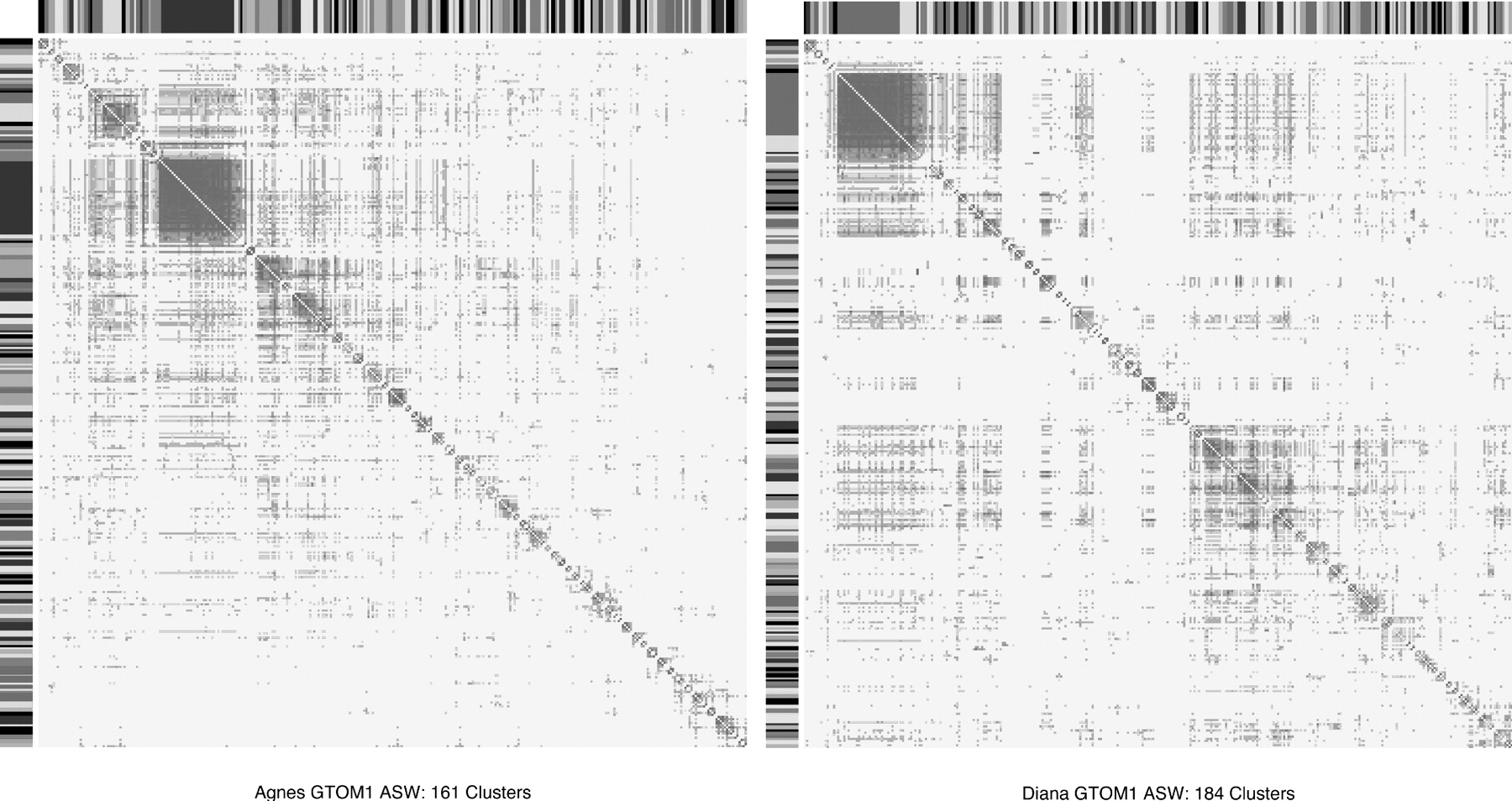
Heatmaps for Agnes and Diana clusters based on GTOM1 with ASW criterion for number of clusters. Clusters of proteins are represented by color bands in the margins. Distances between proteins are depicted by colors in the plot. Small distances between proteins are assigned darker colors and large distances are assigned lighter colors. Perfect clustering would result in a heat map with all dark colors concentrated within non-overlapping diagonal blocks. The concentration of dark colors (small distances) within diagonal blocks shown here indicates reasonable clustering of these proteins.
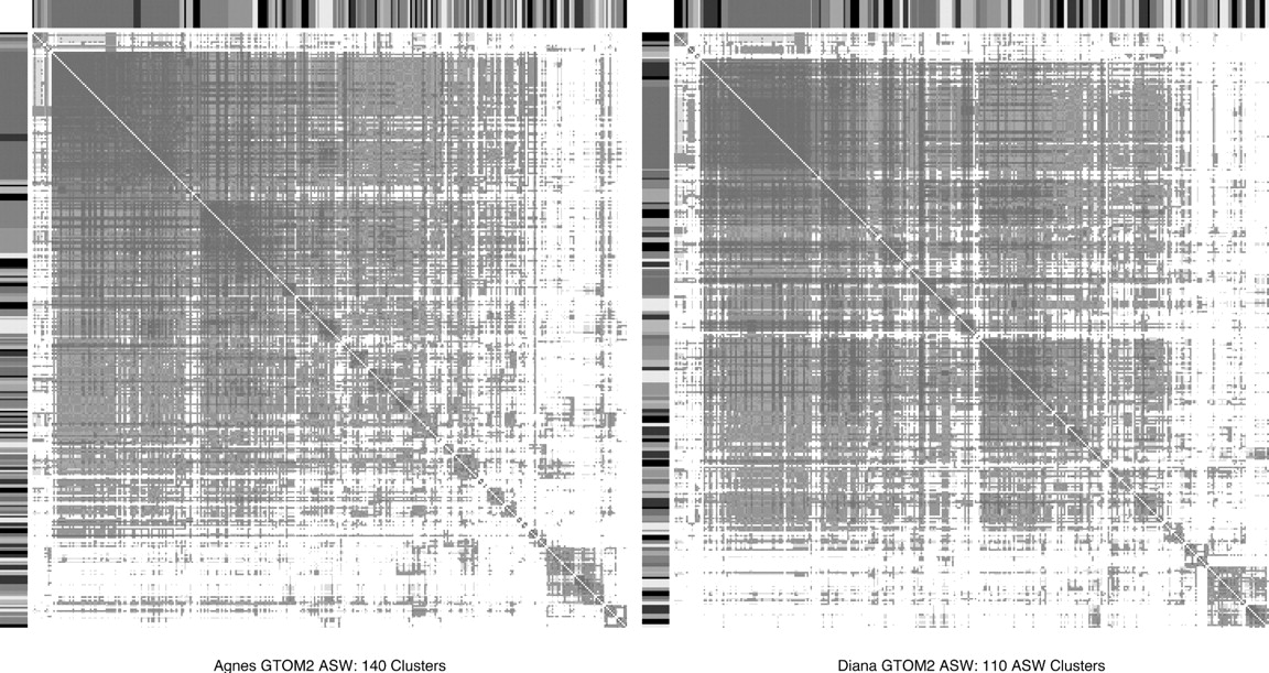
Heatmaps for Agnes and Diana clusters based on GTOM2 with ASW criterion for number of clusters. Since dark areas are not concentrated along the diagonal, these heatmaps show that GTOM2 with Agnes and Diana do not have clearly defined clusters.
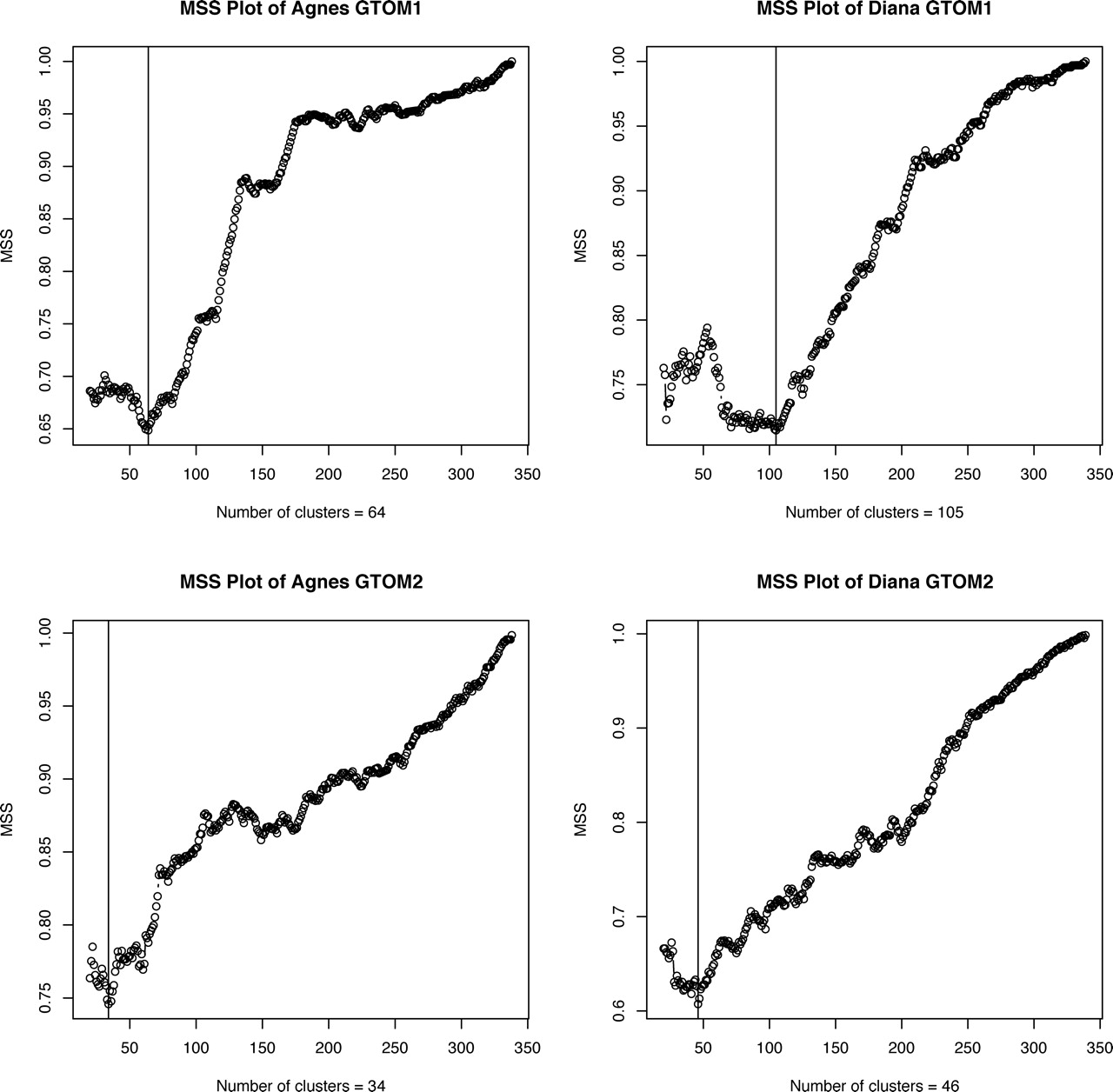
MSS vs cluster size for Agnes and Diana clustering based on GTOM1 and GTOM2. The optimal number of clusters is marked by the vertical line in each plot.

Heatmaps for Agnes and Diana clusters based on GTOM1 with MSS criterion for number of clusters.
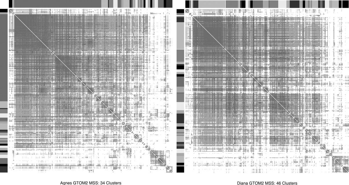
Heatmaps for Agnes and Diana clusters based on GTOM2 with MSS criterion for number of clusters.
Footnotes
Research partially supported by NIH HL070588 Project 1 (SRG).