Towards Improved Cancer Diagnosis and Prognosis Using Analysis of Gene Expression Data and Computer Aided Imaging

Abstract

With the increasing cost effectiveness of whole slide digital scanners, gene expression microarray and SNP technologies, tissue specimens can now be analyzed using sophisticated computer aided image and data analysis techniques for accurate diagnoses and identification of prognostic markers and potential targets for therapeutic intervention. Microarray analysis is routinely able to identify biomarkers correlated with survival and reveal pathways underlying pathogenesis and invasion. In this paper we describe how microarray profiling of tumor samples combined with simple but powerful methods of analysis can identify biologically distinct disease subclasses of breast cancer with distinct molecular signatures, differential recurrence rates and potentially, very different response to therapy. Image analysis methods are also rapidly finding application in the clinic, complementing the pathologist in quantitative, reproducible, detection, staging, and grading of disease. We will describe novel computerized image analysis techniques and machine learning tools for automated cancer detection from digitized histopathology and how they can be employed for disease diagnosis and prognosis for prostate and breast cancer.

Introduction and Motivation

In the last decade, the nature of diagnostic health care has changed significantly because of an explosion in the availability of patient data for disease diagnosis. Traditional methods of analysis of cancer samples were limited to a few variables, usually stage, grade and the measurement of a few clinical markers such as ER, PR, HER2 for breast cancer, PSA for prostate cancer, etc. The pathologist was trained to synthesize this information into a diagnosis which would help the clinician determine the best course of therapy. These data were also used to try to understand the molecular basis of cancer with the goal of improving therapy. In this paper we describe how the availability and analysis of a much larger set of variables combined with sophisticated imaging and analysis techniques promise to radically change this traditional paradigm.

It has always been accepted that cancer is a complex disease which we do not yet fully understand. The same treatment applied to two patients with very similar clinical presentation often has vastly different outcomes. A part of this difference is undoubtedly patient specific and another part is the result of our limited understanding of the relationship between treatment, disease progression and clinical presentation. However, some of the uncertainty results from the current relatively crude systems of tumor classification and the piecemeal approach to clinical data as used in diagnosis and treatment. There is a consensus among clinicians and researchers that a more detailed approach that effectively combines data from multiple diagnostic modalities to identify clinically relevant tumor classes will lead to better patient care and more effective therapeutics. At present, diagnostic information available to the clinician includes i) molecular features of tumor cell and microenvironment as measured by gene expression profiling, RT-PCR and FISH, and immunohistochemistry, ii) microscopic architectural/structural features of the tumor cellular architecture and microenvironment, as captured in histological features, iii) macroscopic features of tumor 3-D tissue architecture and vascularization, and extent of local and distant metastasis as measured by imaging techniques such as high resolution CT scans and dynamic contrast enhanced (DCE) MRI, and iv) its metabolic features, as seen by metabolic or functional imaging modalities such as Magnetic Resonance Spectroscopy (MRS) or Positron Emission Tomography (PET). It is likely that these different modalities are not independent: the gene expression profile of a tumor may well be reflected in its histology and perhaps its macroscopic architectural and metabolic features. The general goal of the analysis of tumor data is to apply computational algorithms to these different modalities of diagnostic data to understand how these features are interrelated and translate this understanding into defining clinically relevant disease categories, with the ultimate aim of improving therapy. In this paper we describe our own modest efforts towards this goal.

Microarray Analysis of Breast Cancer: Disease Subtypes with Distinct Biology and Recurrence Risk

In spite of the availability of vast amounts of breast cancer microarray data, the prevalent view seems to be that this technology provides only a noisy and confusing snapshot of the state of a tumor. This is an unfortunate and incorrect conclusion whose origin can be traced to the initial use of non-robust analysis techniques and the use of feature sets (genes used in the analysis) that were uncorrelated with the known biology of the disease. Because of this, these early studies were unable to show significant improvements compared to predictions that could be made using standard clinical markers such as stage, grade, ER, PR and HER2 status. Fortunately, recent developments, starting with the acceptance of the Oncotype DX panel into clinical practice, promise to overturn this prejudice. In what follows, we will give an example of a novel technique which combines clinical knowledge about breast cancer with robust feature selection and unsupervised consensus ensemble clustering techniques to improve disease stratification, risk and prognostic analysis. We will show that it is possible to devise techniques which combine knowledge of the pathology of breast cancer with new methods applied to microarray data to identify subclasses of disease that are strongly correlated with long-term survival and identify distinct and robust molecular signatures for these subclasses. The methods we describe are designed to be stable to data and feature perturbation and can easily be used to classify unseen data. Finally, these methods provide better (more informative) prognostic predictions than currently available panels for recurrence risk (such as Oncotype DX and MammaPrint). We also see preliminary indication that the subclasses of HER2+ disease identified by the analysis respond very differently to therapeutic agents such as Herceptin. This observation may provide clues to the identification of new therapeutics for the Herceptin non-responsive class of HER2+ breast cancer patients.

Since the methods we use are not described in detail in any one place, we describe them in some detail (see section titled, “Unsupervised Consensus Ensemble Clustering for the Analysis of Gene Expression Data”) as they were applied to a breast cancer microarray data. However, the methods are quite general and can easily be adapted to other types of tumors.

Status of Breast Cancer and Its Analysis by Microarray Profiling

There are over 200,000 cases of invasive breast cancer diagnosed each year in the United States. Although advances in diagnosis and treatment have led to improvements in survival, over 40,000 women die each year from this disease. It is becoming increasingly clear that breast cancer is not a single disease, but instead, consists of multiple subtypes with distinct clinical behaviors and treatment approaches. Approximately 60–70% of tumors express the estrogen receptor (ER), and are susceptible to treatments targeting the estrogen signaling pathway (1, 2). Approximately 20–30% of human breast cancer have amplification of the human epidermal growth factor receptor-2 (HER2) and are treated by Herceptin and other agents that target the HER2 transmembrane receptor tyrosine kinase (3). However, there remains significant heterogeneity in both natural history and treatment response in tumors with similar clinical classification (1–3).

Gene expression analyses have provided insight into this clinical heterogeneity. Supervised learning methods applied to gene expression data have resulted in several gene panels predictive of risk that are currently in clinical use (4, 5). In a different approach, unsupervised clustering of gene expression data using simple hierarchical clustering (6, 7) has identified breast cancer subtypes with distinct gene expression profiles correlated with recurrence risk and survival. The overall classification that has emerged from these early studies divides breast cancers into Luminal A (ER+ with good prognosis), Luminal B (ER+ with poor prognosis), Basal-like (ER-, PR-, HER2-) and HER2+ (HER2+, ER-). These subtypes have been validated in several subsequent studies (8–12).

Despite these advances, it is not clear that these classifications are an advance over simple methods already in use in the clinic based on standard histological analysis. Indeed, as we will show later, relatively expensive panels which are now in clinical use and which were developed based on gene expression data analysis (such as Oncotype DX) give results which may not be improving much on simpler predictions based on ER, PR, HER2 status and histologic grade.

The reason it is difficult to identify optimum markers for stratification and recurrence risk in gene expression data is that most breast cancers are ER+, and many genes are coordinately regulated by ER. As a result, data filtering methods (13–17) are strongly biased towards estrogen pathway genes. When clustering methods are applied to such a gene set, they tend to divide samples along an ER+/ ER- split (e.g., see (6)). Although this approach works well to distinguish Basal-like Cancers (BLC) from the luminal subtypes, it does not work as well for clustering HER2+ tumors. Only HER2+ tumors that are also ER- cluster into a unique subtype. The HER2+ tumors which are also ER+, which account for roughly 50% of HER2+ breast cancer, tend to cluster among the Luminal B, i.e., with other high grade ER+ tumors. However, such a splitting of HER2+ tumors into ER+/ER- clusters may not be biologically or clinically relevant and might arise simply from a combination of biases in sampling, gene choice and clustering method (see (18) and (19) for an analysis which suggest such a scenario based on a reanalysis of the data from (20) and (21), respectively).

Optimized Classification of Breast Cancer into Subtypes from Gene Expression Data

We have developed a general classification method that uses both clinical information and gene expression analysis to robustly identify subtypes of breast cancer which can be easily extended to other cancers. For breast cancer, our approach (18) is to first separate HER2+ samples using either clinical test results (IHC or FISH), or if these are unavailable, using gene expression levels for four Her2/neu amplicon genes (Her2/neu, GRB7, STARD3 and PPARB). This is followed by an analysis of the HER2+ and HER2-subtypes to find further substructure using a robust classification method (described in (18) and (19)) based on principal component analysis (PCA) and consensus ensemble clustering (22–26).

The robust unsupervised consensus ensemble clustering techniques we have developed are described in detail (see section titled Unsupervised Consensus Ensemble Clustering for the Analysis of Gene Expression Data) and were used to classify the 286 samples in the breast cancer data set from Wang et al. (20). We chose this data set because all cases were early stage (lymph node negative), were treated with only surgery and radiation therapy, and had long-term clinical follow-up. Since all these cancers were from a similar stage and were given similar treatment with no adjuvant therapy, the clinical outcome of these tumors should reflect the underlying biology. This means that the interpretation of results from the gene expression analysis would not be confounded by varying stage and treatment.

Our methods identified a total of eight robust BCA subtypes. Within the HER2- cases, we found one Luminal A cluster (ER+, good prognosis), three luminal B clusters (ER+ with mixed prognosis, which we will label LB₁, LB₂, and LB₃) and two Basal-like clusters (BA₁, BA₂). The HER2+ cases also clustered into two clear subtypes (HER2+ _I and HER2+ _NI) with significantly different distant metastasis-free survival rates (86% and 42%, respectively). However, the major pathway distinguishing these two subtypes of HER2+ was not estrogen signaling. Instead, the data demonstrated a strong upregulation of a wide variety of cytokines and other lymphocyte-associated genes in the good prognosis subtype HER2+ _I, suggesting that the presence of a lymphocytic infiltrate in node negative HER2+ tumors is correlated with an improved natural history.

Clinically, HER2+ breast cancer has a heterogeneous natural history and a heterogeneous response to treatment. Although HER2+ breast cancer is thought to have poorer prognosis than Luminal A breast cancers, it is clear from our analysis that subsets of early-stage HER2+ breast cancer associated with a prominent lymphocytic infiltrate have very good prognosis. Moreover, only about 50% of HER2+ primary untreated breast cancer show a measurable response to treatment with Herceptin, suggesting that not all HER2-amplified tumors respond to HER2-targeted therapy (27, 28). At present the vast majority of patients with HER2+ breast cancer is being treated with Herceptin-containing regimens, including growing numbers of early stage patients. It is likely that only a subset of these patients is actually having benefit from this potentially morbid and expensive treatment. Interestingly, there is some data to suggest that the presence of lymphocytic infiltrate at diagnosis may predict response to single agent Herceptin (28). These data suggest that understanding the biology of immune infiltrates in HER2+ breast cancer can lead to significant implications for the treatment of women with these cancers.

Figure 1 shows the metastasis-free Kaplan-Meier survival curves for the two HER2+ subtypes identified by our method. The difference in long-term rates for metastasis between HER2+_I and HER2+_NI is highly significant (P < 0.01). In contrast, the recurrence in the HER2+ group was not well separated by ER status (data not shown). These results suggest that ER status is not a good discriminator of recurrence in early stage HER2+ cases treated with local therapy alone.

A signal-to-noise ratio test comparing HER2+_I and HER2+_NI identified genes that were differentially expressed between these subtypes. The genes over-expressed in the good prognosis HER2+_I subtype included many cytokines, immunoglobulins and other lymphocyte-associated genes. A Gene Ontology analysis using the GSEA tool (29) showed an enrichment of the “immune support” pathway involving T-cell activation, inflammation mediated chemokine and cytokine signaling and B cell activation (P < 0.01). A cluster of chemokine genes adjacent to the HER2 amplicon, which included CCL2, CCL5, CCL8, CCL13, CCL18, CCL23, were among the top genes up-regulated in HER2+_I. Their presence suggests that the size of the Her2/neu amplicon in HER2+ breast cancers may play a role in inducing/eliciting the lymphocytic infiltrate. However, there were also other up-regulated and lymphocyte-associated genes identified by our analysis which were not located near the HER2 amplicon. This up-regulation of many cytokines, chemokines and other lymphocyte-associated genes in the HER2+_I subtype was highly suggestive of the presence of a strong lymphocytic or immune infiltrate in this subgroup of tumors.

Confirmation of the Presence of an Immune Infiltrate in HER2+_I.

Tumor RNA used to generate gene expression profiles in the Wang et al. data set (20) (and indeed in most breast cancer gene expression data sets) comes from bulk tumor. Microarray analysis of such tumor specimens tests not only the tumor cells but also non-tumor components of the tumor microenvironment. A likely explanation for the enrichment of lymphocyte-associated genes in HER2+_I was that these tumors have a strong lymphocytic infiltration. To directly test this hypothesis, we analyzed an independent set of HER2+ tumors for which both histology and gene expression data were available. This data was obtained from a previously reported (30) set of 21 HER2+ tumors which were part of a phase II neo-adjuvant trial of treatment with trastuzumab (Herceptin) and vinorelbine. Prior to treatment, core biopsies were obtained and separate cores were processed for histology and for RNA extraction, amplification and hybridization to Affymetrix U133a arrays to generate results for 21 HER2+ tumor samples.

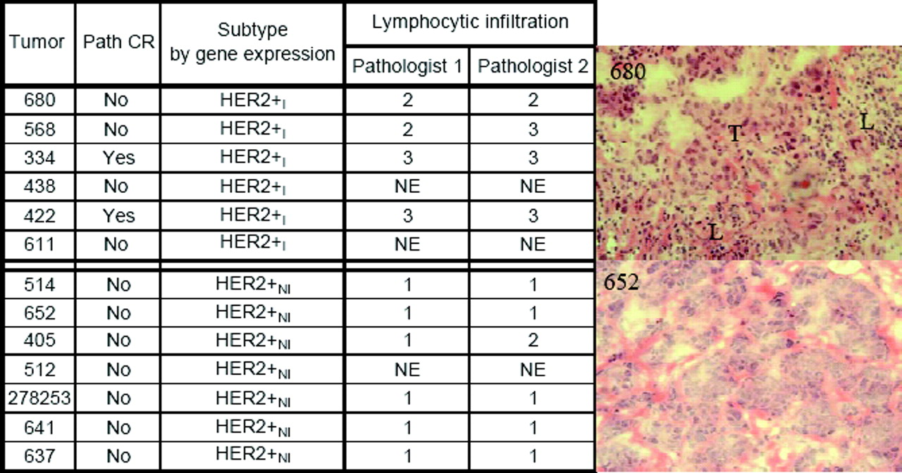
Our analysis of the gene expression data on these 21 samples split the new tumor samples into 3 clusters: cluster 1 had 6 samples with a strong lymphocyte-associated gene signature and was classified as HER2+_I; cluster 3 had 7 samples and little to no expression of these lymphocyte-associated genes and was classified as HER2+_NI; and cluster 2, with 8 samples, had a mixed signature, and was not easily classifiable as either HER2+_I or HER2+_NI. Core biopsies, being by nature small specimens, have more variable sampling of the tumor microenvironment and biases introduced by cDNA amplification. We believe that this is the reason it is difficult to clearly stratify the subset of HER2+ tumors in cluster 2.

Hematoxalin and eosin (H&E) stained frozen sections of pre-treatment core biopsies from these tumors were examined independently in a blinded fashion by two breast cancer pathologists who had no knowledge of the gene expression classification and who were asked to score for the presence of a lymphocytic infiltrate using a rating of 1 to 3, with 1 signifying minimal to no lymphocytes associated with tumor regions; 2 signifying moderate lymphocytic infiltrate present; and 3 signifying a marked lymphocytic infiltrate. The Fisher Exact test was used to generate the P values for the combined pathologists’ scores. When these pathologists’ scores were compared to the gene expression classification, the tumors classified as HER2+_I all scored as having a moderate to marked lymphocytic infiltrate, and almost all the HER2+_NI scored as having no or minimal lymphocytic infiltrate (see Fig. 2). The differences in histological scoring of lymphocytic infiltration between these groups was highly statistically significant based (Fisher Exact test overall P value < 0.0001). These data are consistent with the HER2+_I tumors being associated with a prominent lymphocytic infiltrate.

Correlation of Immune Infiltrate with Neo-Adjuvant Therapy with Trastuzumab (Herceptin) and Vinorelbine.

Of the 6 HER2+_I tumors in cluster 1, two had a documented complete pathologic response (pCR) to neoadjuvant treatment with trastuzumab and vinorelbine. In the 7 HER2+_NI tumors (cluster 3), there were no pCRs. In cluster 2, there was one documented pCR and this tumor showed histologic evidence of extensive lymphocyte infiltration in the original diagnostic biopsy, but a mixed gene expression profile. These data are suggestive that the presence of a lymphocytic infiltrate may predict which tumors will respond well to Herceptin-based treatment regimens. The positive correlation between better survival for HER2+_I patients and response to Herceptin suggests the disturbing possibility that patients in the HER2+_NI subtype may be getting little benefit from Herceptin therapy.

The Oncogene IKBKE Is Over-Expressed in HER2+_I and Basal-Like Subtypes.

The robust expression of a variety of cytokines and cytokine receptors in HER2+_I suggests that activation of cytokine-dependent cellular signaling may be a hallmark of these tumors. The NF-κB pathway is a central pathway in cellular growth signaling. A recent study (31) showed that IKBKE (IKKε), a kinase in the NF-κB pathway, is an oncogene over-expressed in a subset of breast cancers. They also found an allelic gain of Chr-1q in cell lines and tumors where IKBKE was over-expressed.

Using three independent datasets (20, 32, 33), we found that IKBKE is up-regulated only in the HER2+_I breast cancers and not in HER2+_NI. IKBKE is also up-regulated in the Basal-like subtype of breast cancer (see discussion below for further analysis of Basal-like subtypes). Data from one such analysis is shown in Figure 3. Interestingly, as shown in the figure, if data from all HER2+ tumors is combined, there is no clear IKBKE signal in the combined set; the signal only shows up when the HER2+ samples are subdivided into the two subgroups identified by our robust clustering analysis. Moreover, as suggested in (31), we also find that IKBKE correlates with a lymphocytic signature in HER2+_I and with the interferon pathway in the Basal-like subtypes (more prominently in BA₁ than BA₂—see below). Mapping the gene expression data to chromosomes, we found that the HER2+_I subtype exhibits amplicons in the Chr1q32 region (FLJ13310, CR2, CR1, IL10, IL19, IL24, FAIM3, PIGR, YOD1, PFKFB2, C4BPA) in the vicinity of the IKBKE gene, as well as in the Chr1q23 region. The latter region includes interferon gamma, immunoglobulin and several antigen genes: FCRL2, KIRREL, ELL2, CD1D, CD1A, CD1C, CD1B, CD1E, SPTA1, MNDA, PYHIN1, IFI16, AIM2, IGSF4B, FY, FCER1A. These results suggest a possible causal connection between immune activation in HER2+_I and IKBKE/NF-κB activation. Support for this link between NF-κB activation and HER2+cancers includes reports that HER2+ tumor specimens show nuclear localization of p65 in tumor cells (34). Pharmacologic or molecular inhibition of NF-κB activation inhibited growth of HER2+ cell lines, suggesting that NF-κB is required for continued growth of at least a subset of HER2+ breast cancers (34, 35).

Biological Basis of Lymphocytic Infiltrate in HER2+_I.

Our results support prior clinical observations (36, 37) that the histological presence of a lymphocyte infiltrate identifies a subgroup of early-stage HER2+ breast cancer that have a remarkably good natural history when treated with local therapy alone. In these prior studies, it was noted that the difference in natural history was limited to node negative HER2+ tumors, suggesting that the presence of a lymphocytic infiltrate may affect likelihood of metastasis in early lesions. Moreover, the correlation of lymphocytic infiltrate with better outcome was not seen in HER2- tumors, suggesting that the biologic basis, cellular makeup, and clinical impact of lymphocyte infiltration may be quite different in different subtypes of breast cancer.

The presence of specific immune infiltrates has also been associated with improved prognosis in some other cancer types, including ovarian cancer and colon cancer (38–40). However, the presence of certain T-cell subsets have also shown to negatively impact prognosis in other studies, suggesting that the exact composition of the immune infiltrate and/or its specific interactions with tumor cell biology may vary significantly in different tumors (41, 42). It may be that certain classes of cancers may induce distinct types of lymphocytic infiltrate that impact their natural history. In keeping with this, it has been reported that the immune infiltration in HER2+ tumors has a preponderance of macrophages, while immune infiltrate in HER2- tumors was composed mostly of T-cells (36, 43). Recently, infiltration of breast cancers with regulatory T-cells was shown to be associated with poor prognosis; however, it is not clear if these T-reg infiltrates were found only in a specific subclass of breast cancer (43). The biological basis for the lymphocytic infiltrate in these diverse tumor types, their exact nature and composition, and their impact on natural history needs further investigation.

The collection of tumors we examined were all early stage (lymph node negative) and none received adjuvant therapy. Thus we do not know if the subclasses of tumors we identified will have different responses to adjuvant treatment. For example, the question of whether the two HER2+ subgroups will respond differently to chemotherapy and/or trastuzumab remains open. One recent study suggests that HER2+ tumors with lymphocytic infiltrates may have high response rates when treated with trastuzumab alone (28). As we have shown above, in the subset of tumors we analyzed from a neoadjuvant trial of trastuzumab and vinorelbine, there also seems to be an association with lymphocytic infiltrate and achieving a complete pathologic response.

Our results raise multiple questions about the biology of HER2+ breast cancers. Why do certain tumors have a lymphocytic infiltrate? Does the size of the HER2 amplicon, i.e., whether it encompasses the nearby cytokine rich region on 17q, correlate with the lymphocytic infiltration? What is the exact composition of this infiltrate in different tumor subtypes? Is the tumor or tumor-associated stroma secreting key cytokines responsible for lymphocyte chemotaxis? Does the infiltrate reflect an autoimmune recognition of the tumor? Are the infiltrating lymphocytes providing a crucial growth factor for the tumor or tumor-associated stroma?

Although multiple studies in the past have looked at the presence of inflammatory and immune cells in breast cancer (43–49), these were mostly done without classification of breast cancer into robust subtypes. Thus the data are hard to interpret, and indeed conflicting results on the biological nature and clinical significance of these infiltrates have been reported. B-cell, T-cell, macrophages, and dendritic cells have been found to be associated with “invasive breast cancer” and have been reported to be associated with both good and bad prognosis. Our novel analysis suggests that by analyzing the nature and significance of immune infiltrates in biologically distinct subclasses of breast cancer identified by this analysis, it may be possible to gain new insights into the role of immune infiltrates in these tumors.

Subtypes of Luminal and Basal-Like Cancers and Their Risk of Distant Metastasis

In the Luminal cancers, we found four robust subtypes, with metastasis-free-survival rate above 79% for one of the subtypes and below 60% for the rest. Following Sorlie et al. (9), we labeled the “good prognosis” subtype Luminal A (LA) and the three “poor prognosis” clusters collectively as Luminal B (LB) or separately as LB₁, LB₂ and LB₃. The Kaplan-Meier curves for the Luminal A and Luminal B subtypes are shown in Figure 4. Within the Basal-like (ER-, PR-, HER2-) samples we identified two subtypes BA₁ and BA₂, with average recurrence rates of 32% and 41%, respectively.

It is clear from Figure 4 that samples in the four Luminal subtypes, when treated only with radiation following surgery, have very different long-term risk of metastasis, with LA having the lowest risk (21%) and LB₂ the highest (55%). The response of these subtypes to long-term therapy with Tamoxifen or similar agents remains to be tested. For the Basal-like cases, the conclusion is that although BA₁ and BA₂ are distinct molecular subtypes of disease, they do not display any significant difference in natural history under local treatment alone, at least for these early stage tumors (Fig. 5 ). However, given the absence of any specific targeted treatments available for Basal-like breast cancers, the identification/validation/characterization of the genetic profiles of BA₁ and BA₂ may be quite important. A variety of novel treatment strategies for BLC have been proposed. These include using specific categories of DNA damaging agents, such as cisplatin, EGFR targeted therapy, and broad spectrum tyrosine kinase inhibitors (50–52). As early phase clinical trials testing these and other strategies are either under way or being planned, it may be important to distinguish between BA₁ and BA₂ within these trials and determine whether these subtypes will have different responses to the treatments administered in these trials. In our preliminary results, we have discovered that almost all BRCA1 cases fall into the BA₁ subtype, have amplification of the NF-kB and IFN pathways and may be sensitive to tyrosine kinase inhibitors like Dasatinib (unpublished).

Comparison of Subtypes with Oncotype DX and MammaPrint Panels

The Oncotype Dx and MammaPrint gene panels (4, 5, 53, 54) have been proposed to distinguish good prognosis from bad prognosis breast cancer patients under different conditions and treatments. Strictly speaking, these apply only under their specific conditions; e.g., the Oncotype DX panel of Paik et al. is specific to recurrence in node negative, ER+ patients treated with Tamoxifen. Nevertheless, it is instructive to apply these panels to our subtypes.

Figure 6a show the ranges of raw scores for the ER+ samples in our subtypes for the Oncotype DX panel (5). To make a precise comparison, it is necessary to have the measured RT-PCR values for the 21 genes for all the samples, correct for possible variance bias for each gene and compute a normalized score using the scaling in (5). In the absence of such detailed data, for the ER+ samples, we averaged all correlated probe values for each gene per array followed by standard normalization of each gene across samples before using the weights in the Oncotype DX panel to compute a raw score for each sample. This is the scale shown for the Oncotype DX results in Figure 6a. It should give the correct relative recurrence risk score as an increasing function of the un-normalized (raw) score. The order of increasing risk predicted by the Oncotype DX panel is: Luminal A, LB₃, LB_1, LB₂, HER2+_NI, HER2+_I. Note that the relative order of risk in the Luminal B does not agree with the actual results in Figure 4 and the risk for the HER2+ subtypes is reversed from the actual measured values in Figure 1 . In Figure 6b we show the ranges of subtype scores using the MammaPrint panel (4, 54). Once again, although the Luminals cases are identified to have lower risk than the BLC or HER2, the relative recurrence risk for BLC and HER2 are reversed compared to Oncotype DX and the relative recurrence risk of the HER2+_I and HER2+_NI subtypes is once again inverted compared to measured values. A striking feature of Figures 6a, 6b is that the range of scores within a subtype is small, with most of the variability being between subtypes. This suggests that the Oncotype DX and MammaPrint stratification may be a surrogate for the global subtypes Luminal/Basal-like/ HER2+ which may be identified using simpler standard clinical tests (ER, PR, HER2, grade) alone. If this is the case, then these panels may not be adding much prognostic information within individual subtypes.

Application of Computerized Image Analysis Tools for Detection of Prostate and Breast Cancer

When a patient is suspected of cancer, the typical diagnostic procedure involves sending a biopsy specimen to a pathology lab for manual visual analysis, confirmation of the condition, and classification and grading of the cancer (if present). In the United States, approximately one million prostate cancer (CaP) biopsies are done every year, each one producing 10–15 tissue samples for analysis. With an overall CaP diagnosis rate of approximately 20%, pathologists across the country spend a large fraction of their time looking at benign tissue, which in most cases is easily distinguishable from cancer (55). This represents a huge waste of time and resources that might be better spent analyzing patients who actually have CaP, or to focus on the cases where the disease is difficult to identify/classify or presents with non-standard features.

A solution we propose to deal with this issue is to develop a computer aided diagnosis (CAD) system where an algorithm is used to guide and corroborate a pathologist in manual classification of digitized tissue images. At ×40 resolution, a single biopsy tissue sample when digitized may result in a digital image which is 10 GB in size. To be practical, a CAD system must quickly and efficiently analyze digitized images of histology and determine whether there are any cancerous regions present in the image. Such a system can improve the field of cancer research by: i) creating quantitative image metrics against which tissue patterns may be compared, thus reducing the variability seen in current diagnostic practice, ii) enabling pathologists to analyze tissue samples in greater detail, leading to faster treatment, and iii) improve patient diagnosis.

To accomplish this goal, we have utilized a hierarchical, multi-scale system that mimics the search methodology of a pathologist to analyze large histopathological images quickly and efficiently (56). We use a large set of texture features to describe each pixel in the image, and based on those feature values, train a classifier to distinguish between benign and cancerous pixels. Although the optimization of parameters may change from application to application, this basic framework can be applied to many tissue types that are currently examined manually. We will describe below how we have applied these methods to prostate and breast biopsy tissue samples.

Prostate Cancer Detection from Digitized Histopathology Obtained via Needle Biopsies

Slides of histological tissue are scanned into a computer using a high-resolution digital whole slide scanner, capable of producing high magnification (×40 optical zoom) images of glass tissue slides. An expert pathologist provides the ground truth for the histological sections. The images and their corresponding ground truths are then decomposed into constituent scales. At each scale, a number of image features is extracted. Exactly which features are used at each scale is determined by empirical offline testing of each feature in the set to determine which perform best in discriminating between the “cancer” and “non-cancer” classes. An example of this feature-selection process is the AdaBoost algorithm (57), which generates a weighted combination of features by choosing those combinations that focus on (and correctly classify) difficult-to-analyze samples. The full set of features includes low-level statistics such as intensity-based statistical features, second-order texture features, and wavelet filtered features, as well as local binary patterns, Laws texture features, and run-length matrix features. Each of these is evaluated at each scale, and those that perform well are kept for use in the finished system.

For pixel classification, we can choose from a number of pattern classification algorithms. It is very difficult a priori to determine which classifier will perform best on a given set of data without empirical tests; consequently our framework does not depend on the use of a specific classifier. For illustration purposes, we describe below a supervised Bayesian classification system. However, we have obtained similar results with other types of classifiers (including Support Vector machines (SVMs), Decision Trees, AdaBoost) as well.

Figure 7 shows results of cancer detection on two slices of prostate histology. The original prostate images in Figure 7(a), (f), with tumor regions denoted in black in Figure 7(b), (g), were analyzed at three image magnifications. The classifier (Bayesian classifier in this case) results (Fig. 7(c)–(e), (h)–(j)) are CaP probability which show the tumor regions as brighter areas, increasing in magnification scale from left to right. The increase in scale allows for greater specificity in classification.

Prostate Cancer Detection from Whole Mount Digitized Histopathology Prostatectomy Specimens

The analysis of whole-mount histological sections (WMHSs) is needed to help determine treatment following prostatectomy and to create the “ground truths’’ of CaP spatial extent required to evaluate other diagnostic modalities (e.g., MRI). The development of CAD algorithms for WMHS is significant for several reasons: i) CAD offers a viable means for analyzing the vast amount of the data present in WMHSs, ii) the consistent, quantified features and results inherent to CAD systems can be used to refine our own understanding of prostate histology, thereby helping doctors improve performance and reduce variability in grading and detection, and iii) the data mining of quantified morphometric features may provide means for biomarker discovery, enabling, for example, the discrimination of patients with and without disease recurrence following CaP treatment.

The CAD system focuses on the discrimination of benign and malignant glands in low-resolution images of WMHSs. This discrimination leverages two biological characteristics: i) gland size and morphology are noticeably different in cancerous and benign regions (58) and ii) cancerous glands tend to be proximate to other cancerous glands. This proximity information is modeled using Markov Random Fields (MRFs) (59).

The steps of the CAD algorithm (60) are as follows: i) gland segmentation is performed on the luminance channel of a color H&E stained WMHS, producing gland boundaries, ii) the system then calculates morphological features for each gland, iii) the features are classified, labeling the glands as either malignant or benign, and 4) the labels serve as the starting point for the MRF iteration which then produces the final labeling.

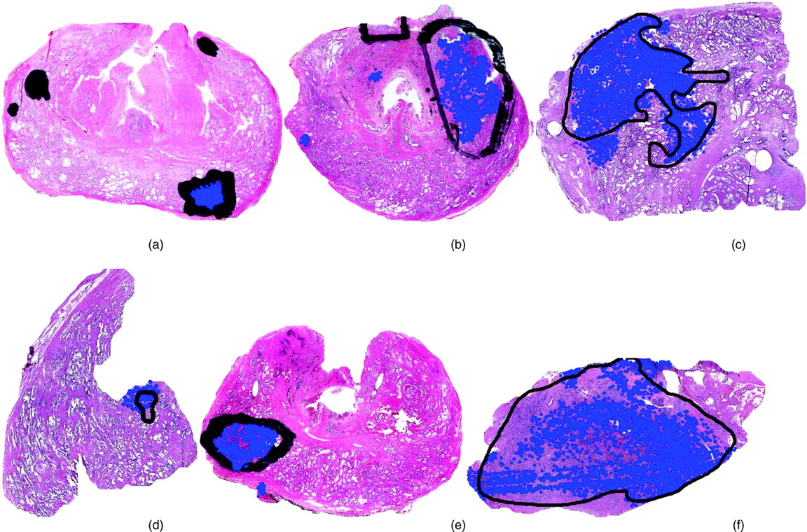
Figure 8(a)–(f) shows the performance of our CAD scheme on six H&E stained WMHSs of the prostate. The black marks indicate the spatial extent of CaP as determined by a pathologist. The CAD algorithm identifies the glands (the prominent white areas) in the WMHSs that are thought to be cancerous. The centroids of these glands are identified with blue dots. Some false positives and false negative are identifiable. However, this is not unexpected for several reasons: i) the CAD system analyzes the images at 20 times lower resolution than that available to a pathologist, ii) the system currently only uses gland area and proximity as features, iii) the truth provided by the pathologist is coarse and approximate and may contain false positive errors, and iv) the goal of the algorithm is not to provide precise results, but to determine which portions of the WHMSs should be analyzed at higher resolution.

Over a cohort of 20 studies we have demonstrated a simple, powerful, and rapid method for the detection of CaP from low-resolution whole-mount histology specimens, which requires only four to five minutes to analyze a 2100 × 3200 image on 2.4 GHz Intel Core2 Duo Processors. Relying only on gland size and proximity, the CAD algorithm highlights the effectiveness of embedding physically meaningful features in a probabilistic framework that avoids heuristics. Figure 9 shows Receiver Operating Characteristic (ROC) curves which show the performance of our CAD system in CaP detection on 20 WMH sections. The dotted ROC line shows CAD performance based solely on gland detection and classification (based on gland area) and without the MRF step. The inclusion of the MRF module significantly improves overall CAD performance (solid dark curve in Fig. 9 ).

Breast Cancer Detection from Digitized Histopathology

Breast cancer, like prostate cancer, is a prevalent problem in industrialized nations, and the analysis mechanisms are largely the same: if a patient is suspected of having a cancerous growth, a biopsy will be performed and analyzed under the microscope.

In our breast cancer study, we took a slightly different approach: instead of calculating pixel-wise probabilities of cancerous growth, we chose a particular image scale (×20 optical magnification) and calculated cancer in a patch-based manner. That is, we obtained regions of fairly homogeneous tissue from a pathologist along with their associated labels (“cancer” or “non-cancer”), and extracted features to represent the image patch. Figure 10 shows some examples of the features we calculated. The texture-based features (middle) are calculated as before, only now we are looking at the average, standard deviation and min/max ratio of the feature values for the region in question. In addition, we extract an entirely new set of graph-based features (right) that capture the arrangement of the nuclei within the image. Using the centroids of the nuclei as nodes, we can construct a Voronoi Diagram, a Delaunay Triangulation, and a Minimum Spanning Tree. From these graphs we calculate the branch lengths, areas of the triangles and Voronoi cells, perimeter, and other features that capture the nature of these graphs.

In this way we can quantify both the texture characteristics and the architectural or nuclear characteristics. The results of the cancer detection algorithm are shown in Figure 11 . We used dimensionality reduction techniques (61) to represent the high-dimensional feature data in a 3-dimensional space. In this image, each dot represents an image, and the distance between two dots is proportional to their similarity: two dots that appear close together represent two images that are similar in high-dimensional space, while two dots appearing far apart are very dissimilar. We would expect that, if the images are indeed from different classes, then they should cluster together. The two class clusters are shown, with black ellipses surrounding them. A classifier drawing a decision plane through these clusters gives a very high accuracy (98%).

Computer-Aided Image Analysis for Disease Prognosis and Survival Prediction

We will give two examples, for prostate and breast cancer respectively, of how image analysis can help improve prediction of disease progression and patient survival.

Computerized Gleason Grading of Digitized Prostate Histopathology

When dealing with a case of prostate cancer, the malignancy of the tumor is typically determined through visual analysis of histological patterns in the tissue. The malignancy is graded according to the Gleason grading scale, which assigns a number from 1 (most benign) to 5 (most aggressive) to different tissue patterns. The Gleason score of a patient is then the sum of the two most prevalent patterns in the image, the “primary” and “secondary” patterns. Higher Gleason scores are associated with worse prognoses since they correspond to more aggressive cancers. However, as with the cancer detection problem, there is still an issue of qualitative analysis leading to inter-and intra-observer variability among pathologists analyzing this tissue. Studies have shown that a significant amount of inter- and intra-observer variability exists between pathologists, especially with respect to identification of intermediate Gleason patterns (grades 3, 4) (62). CAD analysis for quantitative, reproducible Gleason grading on histology will help i) reduce inter- and intra-reader variability and pathologist errors, and ii) help in better prognosis and therapeutic recommendations. Such a system can be valuable for other reasons also, such as the creation of a content-based image retrieval and comparison system, an online database of quantifiable image data for “telepathology” Since image regions that cannot be easily classified as one class or another may constitute a new class, such a system can also aid in the discovery of subtle but unique differences between images of similar grade that might have prognostic of therapy-related differences and provide the basis for revising or augmenting the Gleason grading system (Fig. 12).

The methodology of our proposed system is similar in spirit to that illustrated above, with cancer detection from biopsy samples: i) a set of images is obtained via a whole-slide digital scanner; ii) ground truth is obtained from an expert pathologist in terms of the grade of the tissue sample; iii) samples are digitized based on the structures in the image; and iv) classification or image comparison takes place to identify the grade of a novel sample (63).

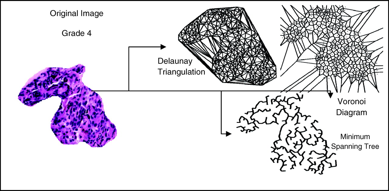
In this system, the features that are used to describe the tissue are augmented from just texture features to include morphology of glands and the arrangement of nuclei, or architecture, present in an image region. We are no longer computing features for individual pixels, but rather, are describing entire patches of tissue with a single set of features. An example of the architectural features is given in Figure 13. In determining the architecture of the nuclei, we employ a graph-based approach: by generating graphs such as the Voronoi Diagram, Delaunay Triangulation, and the Minimum Spanning Tree, we can quantify arrangement by calculating the average graph length, triangle area, Voronoi cell perimeter, and so forth. This gives us a quantitative signature of a particular image patch that can then be compared to other patches or classified using a traditional pattern analysis algorithm.

In Figure 14 , preliminary results showing the differences between quantitative image metrics of Gleason grade 3 (green circles) and grade 4 (blue squares) tissue regions are shown. In the scatter plot, each point represents an image, and its position in space is determined through its feature values. Thus, two images appearing close together are said to be similar in high-dimensional feature space. The two classes under consideration (Gleason grades 3 and 4) separate out nicely, indicating that the feature values we have calculated can accurately discriminate between the two image region types.

Computerized Detection, Segmentation, and Grading of Lymphocytic Infiltration on High Grade HER2+ Breast Cancer Histopathology

Molecular changes in breast cancer (BC) are sometimes accompanied by corresponding changes in phenotype. Therefore, the identification of these phenotypic changes in breast cancer histopathology is of significant prognostic and “theragnostic” value. For example, as we have shown above, robust consensus clustering of gene expression data led to the identification of two subclasses of HER2+ breast cancer, one of which, HER2+_I, was characterized by strong expression of lymphocyte associated genes. This gene expression feature could easily be appreciated in the histology of the tumors; the HER2+ breast cancers with high expression of lymphocyte associated genes had a robust lymphocytic infiltration (LI) that can be identified on visual inspection of standard histology. Early stage tumors that clustered as HER2+_I had a markedly improved natural history, and some data implies that these tumors may respond better to HER2-targeting antibody trastuzumab. Thus a robust method to identify this subset of HER2+ tumors with a robust LI using standard histologic sections and that does not require gene expression profiling could be of great clinical utility. To characterize LI computationally, we present a CAD methodology to automatically detect and quantitatively grade the extent of LI in HER2+ BC histopathology images (64).

The lymphocyte CAD algorithm comprises 3 main stages. First, we employ an automated lymphocyte detection scheme to identify lymphocyte nuclei from surrounding stroma and cancer cell nuclei. A region-growing algorithm initially segments all candidate nuclei (60). Since many cancer cell nuclei are also found, a Bayesian classifier is used in conjunction with a Markov Random Field (MRF) to refine the segmentation (60). The Bayesian classifier calculates features for each candidate nucleus and uses the size and luminance information to distinguish lymphocyte nuclei from cancer cell nuclei. The MRF is an iterative algorithm that models the infiltration phenomenon by incorporating the spatial proximity of lymphocytes in a histopathology image. Using the segmented lymphocytes, a total of 50 architectural (i.e., graph-based and nuclear) features are extracted for each image (65). We construct three graphs (Voronoi Diagram, Delaunay Triangulation, and Minimum Spanning Tree) and calculate 25 graph-based features for each image. The remaining 25 features represent nuclear statistics such as lymphocyte density and nearest neighbor statistics.

For a dataset containing 41 images, we distinguish images with high and low LI by reducing the architectural feature set with non-linear dimensionality reduction (NLDR) and applying a Support Vector Machine classifier (61). We compare our method to two textural feature sets: the popular Varma-Zisserman (VZ) texton-based features and global texture features (65, 66). While the architectural feature set achieves a classification accuracy of 92%, the texton-based and global texture feature sets perform at 60% and 50%, respectively.

Non-linear dimensionality reduction offers the possibility of reducing a high-dimensional feature set into a lower dimensional space, the low dimensional representation of the data in turn reflecting the most important components (61) of the original data. Since it is difficult to conceptualize a high-dimensional space, reducing the features to a 3-dimensional space allows us to visualize the underlying structure of the dataset. Figure 15 shows the stratification of the entire dataset in terms of the low-dimensional architectural feature set and reveals the presence of three distinct stages of LI.

This study demonstrates the ability of a CAD algorithm to automatically detect and quantitatively characterize the nature of LI in breast histopathology. These tasks are of particular importance due to the connection between LI in BC and patient outcome. Furthermore, since the methodology proposed in this study is independent of the underlying biology, it may also be applicable to the histopathology of other diseases. In future work, we plan to extend the clinical relevance of the CAD algorithm by establishing a correlation between degree of LI, prognosis, and “theragnosis”.

Computerized Outcome Prediction Based on Image Analysis of Breast Cancer Histopathology

Breast cancer is a heterogeneous disease, with a wide range of natural histories and responses to different treatments. Measurement of estrogen receptor (ER) expression is a routine part of clinical evaluation of individual breast cancers and is used to guide treatment. However not all ER+ breast cancers respond well to hormonal treatment. A gene-expression based assay, Oncotype DX, has been recently shown to robustly stratify early stage ER+ breast cancer and identify which ER+ breast cancers will have low recurrence rates when treated with adjuvant hormonal therapy. Oncotype DX is expensive and requires specialized facilities to perform, but is now widely used in clinical practice to help identify which early stage ER+ breast cancers will have good long-term prognosis when treated with hormonal therapy alone. Interestingly, standard pathologic grading, based on visual analysis of tumor morphology by trained pathologists, has a strong correlation with Oncotype DX recurrence scores; low recurrence tumors are mostly low grade, and high recurrence tumors are mostly high grade. The correlation of image features (histologic grading) with molecular features (Oncotype Dx score), demonstrates that the image features, if analyzed robustly, can provide similar prognostic information as molecular assays. In other words, tumors with similar molecular features, will have similar image-based features. However a major problem with use of pathologist-assigned histological grade as a prognostic tool is the lack of high reproducibility of histological grading between different pathologists.

To address this problem, we have developed CAD image analysis techniques to obtain a highly reproducible image-based prognostic assay of ER+ breast cancer that can be performed on digital images of standard histology and obtain good correlation between histological image derived signatures and long-term outcome as measured by Oncotype Dx recurrence scores.

For a total of 21 breast cancer studies, unsupervised analysis of image features (nuclear and graph based features) and dimensionality reduction was performed. The cases appeared on a manifold with clear separation of tumors with low, intermediate and high Oncotype DX recurrence scores (Fig. 16 ). This manifold can be reduced to a one-dimensional line to allow calculation of a distance metric which can be used to give each tumor an Image Based Risk Score (IbRiS). In this limited sample set there was nice separation of tumors with high Oncotype DX RS from those with low RS. These data clearly demonstrate that image-based information can provide classification of tumors that can parallel that seen with molecular assays.

Unsupervised Consensus Ensemble Clustering for the Analysis of Gene Expression Data

The unsupervised consensus clustering method we use for the analysis of gene expression data is described below as it applies to the identification of breast cancer subtypes (18). However, it should be obvious from the description that the method is general and can be used to identify stable patterns and/or subclasses in any dataset. The flow chart of the method as applied to the data of (20) is presented in Figure 17.

The first step is data Normalization, whose goal is to standardize the data and correct for inter-array variance in gene expression. Our method is to apply a log2 transformation to the data followed by “median array centralization”. The latter step involves first computing the median of the transformed data for each array across all genes. Next, the “median of medians” (mm) is computed across all arrays. Each entry in each array is then normalized by subtracting mm. This corrects for overall shifts in gene expression within the arrays, forcing them to all have the same median. Sometimes, to correct for high variability in gene expression ranges across the arrays, we also standard normalize (make mean = 0, variance = 1) the expression values of each gene across all samples.

In the next step, we apply principal component analysis to the data, which we will presently explain. However, at this point it is necessary to use as much of the clinical/ biological information as possible to avoid making errors due to sampling or gene choice biases. We explain this issue below in the specific instance of identifying breast cancer subtypes. However, the issue is quite general and the same care must be taken in all cases to ensure that the subtypes identified make sense.

The problem is that the assignment of samples to subtypes is sensitive to sample and gene set bias. In the case of breast cancer, most tumors are ER+, and many genes are coordinately regulated by ER. Data filtering methods are all strongly biased towards estrogen pathway genes because of an overabundance of such tumors in the data (sampling bias) and an overabundance of genes amplified on the array which are related to the estrogen pathway (gene selection bias). Clustering applied globally to such a sample and gene set will divide samples along an ER+/ER- split, which would be a misclassification of some of the subtypes. Specifically, HER2+ samples will split into two groups based on ER levels unless they are separated out first based on the biological insight that HER2+ cases have a completely different disease compared to HER2- cases. The biology of HER2 amplification trumps the biology of estrogen expression. To get the correct disease subtype clustering, the HER2+ cases must first be removed (and analyzed separately) before identification of subtypes in the remaining HER2- cases.

Our approach is to separate HER2+ samples using clinical markers. The best way to do this is to use IHC or FISH to assess HER2 status. If this is not available, one can also identify HER2+tumors to very good accuracy by using the signature of co-amplification of three or more of the Her2/neu amplicon genes. In our case we used the signature: HER2+=co-amplification of three out of four of the mRNA expression levels of Her2/neu, GRB7, STARD3 and PPARB. Once the HER2+ samples are separated, the analysis described below is applied separately to the HER2+ and HER2- cases.

The next step is to apply Principal Component Analysis (PCA) (67) and retain only those genes which contribute most to the variance in the data. PCA is applied to the expression matrix E_ij whose rows are samples and columns are genes or probes. The PCA analysis is done by singular value decomposition of the E matrix after it is centered and scaled to mean 0 and variance 1 per column. The eigenvalues λ_i are sorted in decreasing order and the k largest eigenvalues representing a fraction ρ of the variation in the data are identified by solving [∑_i=1 ^k λ_i] = ρ[∑_i=1 ^Nλ_i] where N is the total number of genes or probes. We typically chose ρ = 0.85. From an examination of the coefficients of the genes in the eigenvectors for these eigenvalues, we chose the subset of genes with coefficients in the top 25–50% in absolute value in the eigenvectors. This collection of genes is used to find robust clusters in the data using unsupervised ensemble consensus clustering.

Unsupervised clustering algorithms divide data into groups such that the intra-cluster similarity is maximized and the inter-cluster similarity is minimized. For gene expression data, unsupervised clustering can be performed for genes, for arrays, or for both. Several types of clustering techniques are available to group data into sets. These may be divided into hierarchical, partitioning, probabilistic and grid-based methods. Ensemble consensus clustering (22, 23) is a relatively recent method which uses a weighted combination of these methods to improve the quality and the robustness of the clusters identified by each individual technique. The consensus ensemble approach is divided into two parts: a method which generates a collection of clustering solutions, and a method that robustly combines the solutions to produce a single “best” clustering solution for the data. Unlike standard clustering techniques whose solutions divide all the data samples into groups, ensemble consensus clustering can sometimes only identify “core” groups of samples within clusters as those samples which are consistently clustered into the same group, independent of perturbations of the data and of the choice of clustering methods used. This allows one to identify strong signatures of gene expression within each core cluster which can then be used to classify the remaining samples. It also allows a robust (perturbation independent) characterization of the gene expressions which distinguish the disease classes identified. Often a study of these genes which have noise independent differential expression between disease classes allows a better understanding of the underlying biological mechanisms driving the subtypes.

We use several techniques to create robust “core” clusters. If the clustering method is stochastic, we reduce the effect of stochastic variation by applying the clustering method repeatedly and taking an appropriate average. To reduce the sensitivity of the results to random variation in the data, we apply each clustering method to multiple sample datasets obtained by bootstrapping both the features (genes/probes) as well as the samples clustered.

The core clusters are identified as those groups whose memberships consist of samples consistently classified into the same group over all the bootstrap and clustering experiments. Many implementations of software for consensus clustering are available: e.g., GenePattern (http://www.broad.mit.edu/cancer/software/genepattern/), R (http://cran.r-project.org/) and conpas (http://www.cs.ucdavis.edu/~filkov/software/conpas/).

The details of the clustering method we use are as follows: For each k = 2,. . . , 50, we create k clusters on re-sampled and random projected datasets based using many individual clustering methods.

Step 1.

We typically generate 150 datasets: 50 datasets by bootstrapping samples, 50 projecting the data onto subsets of genes identified from PCA, and 50 by both sample and gene bootstrapping. We then apply a mixture modeling scheme (implemented in the R package mclust http://cran.r-project.org/ and www.stat.washington.edu/mclust/) to identify the most suitable clustering models for the data (partitioning, agglomerative, probabilistic). The details of the clustering method used are given below.

Partitioning Relocation Methods.

These methods divide data into several subsets and use certain greedy heuristics in the form of iterative optimization to reassign points between the k clusters. The optimization is applied to an objective function defined on unique cluster representatives (e.g., centroid, medoid), which is usually a dissimilarity measure. We applied the following algorithms: a) Partition Around Medoids or PAM (25); b) CLustering LArge Applications (CLARA (25)); c) K-means (68); d) Graph partitioning (69). Clusters produced by centroid methods such as K-means, PAM and CLARA are generally of spheroidal shape. Thus, these methods are suitable for clustering datasets with uniform and relatively low variation among samples. Graph partitioning methods produce clusters in which samples are added in if they are “close” to at least one sample in the candidate cluster. Thus graph partitioning approaches can successfully identify clusters with unequal variance along the feature coordinates (i.e., they can find cluster with a “long” direction).

Agglomerative Methods.

These methods build the clusters by establishing a hierarchical order (25).

One starts by assigning each sample to its own cluster and then recursively merging two or more most similar clusters until a stopping criterion is fulfilled. The similarity between clusters is usually computed based on a linkage metric which reflects the connectivity and similarity between the clusters. In our study we applied hierarchical clustering techniques based on the following metrics for inter-cluster distances: a) Average linkage metric: distance = average distance between the pairs of points in clusters; b) Complete linkage metric: distance = maximum distance between pairs of points in the two clusters. c) Single linkage metric: distance = minimum distance between pairs of points in the two clusters; d) Mcquitty metric: distance = average distance between subclusters of the two clusters; e) Centroid metric: distance = distance between the centroids of the clusters; f) Ward metric: distance = the distance between the centroids of the two clusters weighted by the sizes of the two clusters.

Probability Based Methods.

In these methods, data is considered to be a sample independently drawn from a mixture model of several probability distributions and the clusters are associated with the area around the mean of each distribution. It is assumed that each point is assigned to a unique cluster. The probabilistic clustering method optimizes the log-likelihood of the data to be drawn from a given mixture model.

(EM) Method (70–72).

EM is a two-step procedure which starts by estimating the probability of belonging to a certain cluster. In the next step EM finds an approximation to the mixture model by maximizing the log-likelihood in an iterative way until the convergence to an optimal solution is reached.

Entropy-based-clustering (ENCLUST).

This method (73) starts by dividing the interval associated to each attribute into 1-dimensional bins (cells) and retaining only the cells with a high density. The iterative step consists in creating cells of higher dimensions by joining the cells with low dimension and retaining only those cells which have the entropy below a certain threshold as optimal for clustering.

Self Organizing Maps (SOM).

This method (74) is both a data visualization and a clustering technique which reduces the dimensions of data through the use of self-organizing neural networks. The way SOMs reduce dimensions is by producing a map of usually 1 or 2 dimensions which plot the similarities of the data by grouping similar data points together.

Step 2.

Each method is applied 50 times with different parameter initialization on the full dataset, and once on each of the 150 datasets obtained as described in Step 1. Based on the 200 clustering results, we construct an agreement matrix for each method whose entries m_ij represent the fraction of times the pair of samples (ij) occur in the same cluster out of the total number of times the pair of samples was selected in the 200 datasets.

Using d_ij = 1 μm_ij as the distance between the samples (ij), we apply simulated annealing to find k “core” clusters which satisfy thresholds for both a minimum pairwise distance between clusters and a maximum pairwise distance within clusters. We also require that each pair of samples in a core consensus cluster has an agreement score above some threshold (typically 0.75). At the end of this step, each method yields a best clustering into k core clusters.

Step 3.

For each k, we combine the results from Step 2 across different clustering methods into an agreement matrix to create an overall consensus matrix which is once again analyzed using a distance measure and simulated annealing to identify the final robust core clusters.

The subtypes of breast cancer described in this paper were identified using this method.

Summary and Conclusions

We are living in an exciting time when cancer diagnostics and treatment are becoming more accurate and patient specific. Computerized imaging methods are beginning to assist the pathologist and radiologist in making accurate diagnosis of disease and identify morphological features correlated with prognosis. Molecular profiling of disease promises to help the clinician understand the underlying biology of the disease and suggest new and more effective therapeutics. The motivation for this paper is our conviction that we are at the threshold of an era when predictive, preventive, and personalized medicine (PPP) will transform medicine by decreasing morbidity in cancer. We believe this transformation will be driven by the integration of multi-scale heterogeneous data. The goal of our research and the research of many other scientists is aimed at a future when disease diagnostics will involve the quantitative integration of multiple sources of diagnostic data, including genomic, imaging, proteomic, and metabolic data acquired across multiple scales/resolutions which can distinguish between individuals or between subtle variations of the same disease to guide therapy. Quantitative cross-modal data integration will also allow disease prognostics, allowing physicians to predict susceptibility to a specific disease as well as disease outcome and survival. Finally, the analysis will provide “theragnostics”: the ability to predict how an individual will react to various treatments, thereby providing i) guidance to develop customized therapeutic drugs and ii) enable the development of preventive treatments for individuals based on predicted disease risk. Such a theragnostic profile would be a synthesis of various biomarker and imaging tests from different levels of the biological hierarchy. It would be used as the “signature” of an individual patient, useful in predicting her/his response to drug treatment. A collection of these profiles, followed up over time would provide insights into the disease process and be useful for improvements in developing future treatment options. Our ultimate vision is that someday soon, surgeons, clinicians, pathologists, radiologists and the pharmaceutical industry will join hands with translational researchers from fields outside of traditional medicine, such as Biomedical Engineering, Molecular Biology, Statistics, Computer Science, Chemistry and Physics, to create new datasets and methods of analysis to provide a level of cancer treatment which can reduce this dreadful disease to a chronic condition.

Figure 1.
Kaplan-Meier curves for the HER2+ subtypes showing 86% and 42% long-term distant metastasis free survival for HER2+_I and HER2+_NI, respectively (P < 0.01). A color version of this figure is available in the online journal.

Figure 2.
HER2+_I breast cancers have a prominent lymphocytic infiltrate. Gene expression data were used to stratify a subset of HER2+ breast cancer specimens from a neoadjuvant phase II trial of trastuzumab and vinorelbine into HER2+_I and HER2+_NI subclasses. Hematoxylin and Eosin stained sections of each case were independently scored by two breast cancer pathologists for the presence of lymphocytic infiltration. A score of 1 indicates minimal to no tumor-associated lymphocytes, 2 indicates the presence of a moderate lymphocytic infiltrate, and 3 indicates the presence of a very robust lymphocytic infiltrate. The differences in scores between the two tumor classes are statistically significant (P < 0.0001, Fisher Exact test). The panels to the right show typical histological image of a tumor with a prominent lymphocytic infiltrate (upper right) and a tumor with no lymphocytic infiltrate (bottom right). In the upper right hand panel, a region with tumor cells is marked with T, and a region with prominent lymphocytes is marked with L. A color version of this figure is available in the online journal.

Figure 3.
Mean normalized IKBKE expression levels are shown for different breast cancer subtypes in a combined data set that incorporates samples from (32) and (44). CA, all cancer subtypes; BA, all basal; BA₁, BA₂ are basal subtypes; HER2, all HER2+, HER2+_I and HER2+_NI subtypes; Lum, all Luminal; LA, Luminal A; LB, Luminal B; N, Normal breast tissue. P < 0.001 for HER2+_I vs HER2+_NI. P < 0.0005 for HER2+_I vs N. A color version of this figure is available in the online journal.

Figure 4.
Kaplan-Meier survival curves for (a) Luminal A vs Luminal B and (b) Luminal B subtypes. A color version of this figure is available in the online journal.

Figure 5.
Kaplan-Meier survival curves for the two Basal subtypes BA₁ and BA₂. A color version of this figure is available in the online journal.

Figure 6.
(a) Oncotype DX and (b) MammaPrint panel scores for the 8 breast cancer subtypes identified by our methods. The arrows mark 95% confidence intervals for each core clusters. The relative risk increases from left to right. A color version of this figure is available in the online journal.

Figure 7.
(a), (f): Two digitized histological samples of prostate tissue. (b), (g): Tumor regions corresponding to the histological studies in (a), (f). Classification results are shown increasing in scale from left to right in (c)–(e) and (h)–(j). A color version of this figure is available in the online journal.

Figure 8.
(a)–(f): This figure contains six H&E stained WMHSs of the prostate. The black marks are rough delineations of the spatial extent of CaP. The CAD algorithm estimates which glands in the WMHSs are cancerous. The centroids of these glands are identified with blue dots. A color version of this figure is available in the online journal.

Figure 9.
Receiver operator characteristic curve averaged over 20 trials using randomized 3-fold cross-validation. Solid line indicates CAD performance. Dotted line indicates CAD performance without MRF iteration.

Figure 10.
Examples of breast tissue taken from biopsy. Shown are (a), (d) original patches; (b), (e) grey-level statistical feature image, and (c), (f) a Voronoi graph superimposed on the nuclei in the image. A color version of this figure is available in the online journal.

Figure 11.
Results of region-based cancer detection. Cancer images (red triangles) are in a distinct cluster apart from non-cancer images (black squares). The few outliers are due to image artifacts. A color version of this figure is available in the online journal.

Figure 12.
The Gleason grading scheme. Malignancy increases as tissue patterns change from top to bottom. Reprinted from: Gleason DF. The Veteran’s Administration Cooperative Urologic Research Group: Histologic grading and clinical staging of prostatic carcinoma. In Tannebaum M (ed.) Urologic pathology: The prostate. Philadelphia: Lea and Febiger. 1977. pp.171–198 with permission from Elsevier.

Figure 13.
(a): A digitized histology image of Grade 4 CaP and different graph-based representations of tissue architecture via Delaunay Triangulation, Voronoi Diagram, and Minimum Spanning Tree. A color version of this figure is available in the online journal.

Figure 14.
Distinguishing between Grade 3, Grade 4 CaP on digitized histology via morphometric image features. A color version of this figure is available in the online journal.

Figure 15.
Low-dimensional, architectural feature space showing progression from low (blue circles) to medium (green squares) and high (red triangles) levels of LI. All 41 images in the dataset are plotted with labels determined by an expert clinician. A color version of this figure is available in the online journal.

Figure 16.
(Left panel): Low dimensional embedding of ER+ breast cancer reveals innate structure that corresponds to Oncotype DX recurrence category. Left panel shows embedding in 3-D space with cases lying on a manifold. Right panel shows reduction of manifold to a 1-D line. 𝛉₁ and 𝛉₂ are the optimal thresholds that discriminate between low, medium recurrence and also between medium, high recurrence. A color version of this figure is available in the online journal.

Figure 17.
Flowchart of our unsupervised consensus ensemble clustering method as applied for the identification of molecular breast cancer subtypes. A color version of this figure is available in the online journal.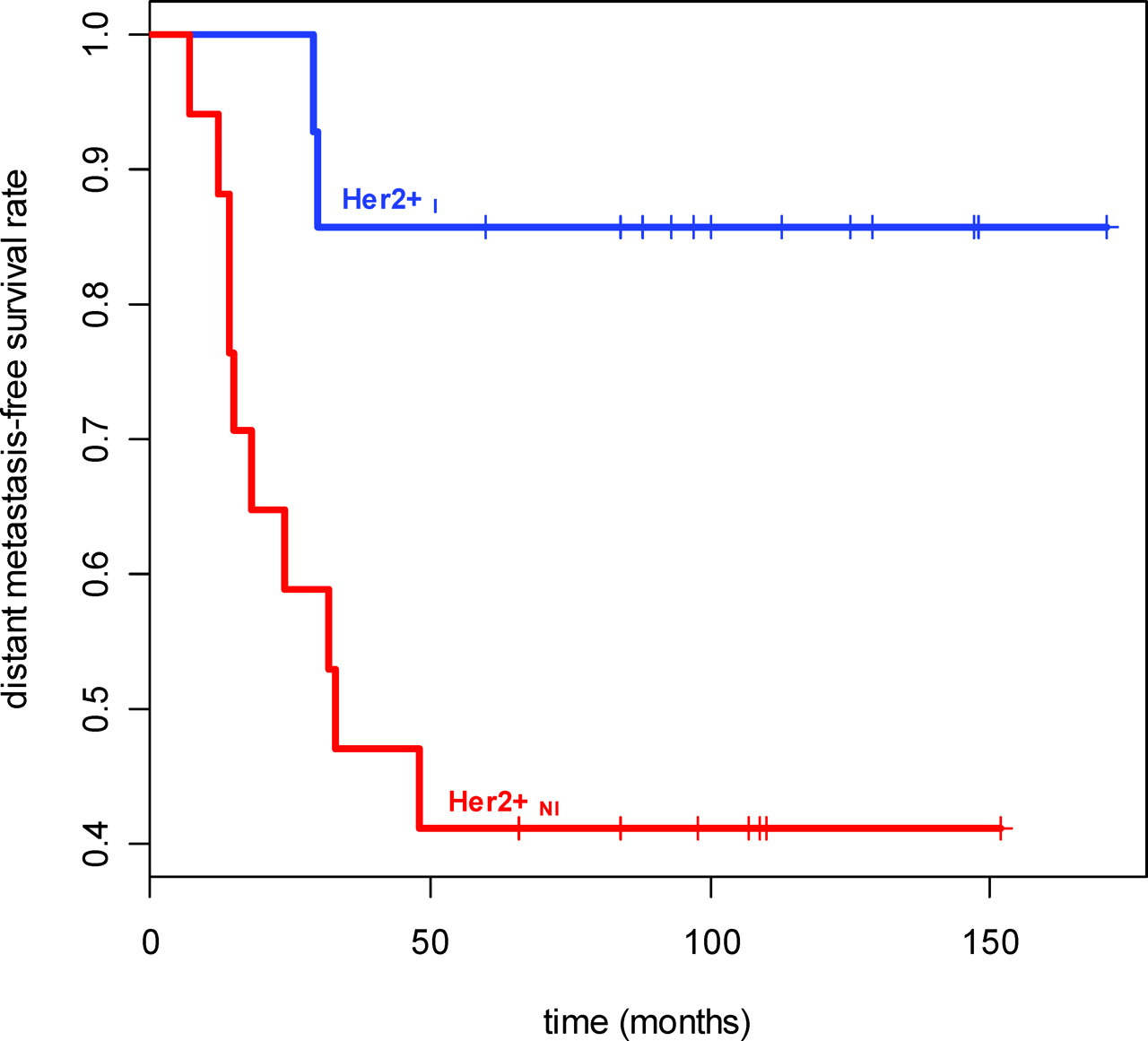

Footnotes

The work of AM was supported by the Coulter Foundation (WHCF 4–29368), the New Jersey Commission on Cancer Research, National Cancer Institute (R21CA127186–01, R03CA128081–01), the Society for Imaging Informatics in Medicine (SIIM), the Life Science Commercialization Award, and the US Department of Defense (427327).

1

Joint first authors.

2

Joint senior authors.

References

Anim JT, John B, Abdulsathar SS, Prasad A, Saji T, Akhtar N, Ali V, Al-Saleh M. Relationship between the expression of various markers and prognostic factors in breast cancer. Acta Histochem 107:87–93, 2005.

Gruvberger S, Ringner M, Chen Y, Panavally S, Saal LH, Borg A, Ferno M, Peterson C, Meltzer PS. Estrogen receptor status in breast cancer is associated with remarkably distinct gene expression patterns. Cancer Res 61:5979–5984, 2001.

Diermeier S, Horvath G, Knuechel-Clarke R, Hofstaedter F, Szollosi J, Brockhoff G. Epidermal growth factor receptor coexpression modulates susceptibility to Herceptin in HER2/neu overexpressing breast cancer cells via specific erbB-receptor interaction and activation. Exp Cell Res 304:604–619, 2005.

van de Vijver MJ, He YD, van’t Veer LJ, Dai H, Hart AA, Voskuil DW, Schreiber GJ, Peterse JL, Roberts C, Marton MJ, Parrish M, Atsma D, Witteveen A, Glas A, Delahaye L, van der Velde T, Bartelink H, Rodenhuis S, Rutgers ET, Friend SH, Bernards R. A gene-expression signature as a predictor of survival in breast cancer. N Engl J Med 347:1999–2009, 2002.

Paik S, Shak S, Tang G, Kim C, Baker J, Cronin M, Baehner FL, Walker MG, Watson D, Park T, Hiller W, Fisher ER, Wickerham DL, Bryant J, Wolmark N. A multigene assay to predict recurrence of tamoxifen-treated, node-negative breast cancer. N Engl J Med 351: 2817–2826, 2004.

Perou CM, Sorlie T, Eisen MB, van de Rijn M, Jeffrey SS, Rees CA, Pollack JR, Ross DT, Johnsen H, Akslen LA, Fluge O, Pergamenschikov A, Williams C, Zhu SX, Lonning PE, Borresen-Dale AL, Brown PO, Botstein D. Molecular portraits of human breast tumours. Nature 406:747–752, 2000.

Sorlie T, Perou CM, Tibshirani R, Aas T, Geisler S, Johnsen H, Hastie T, Eisen MB, van de Rijn M, Jeffrey SS, Thorsen T, Quist H, Matese JC, Brown PO, Botstein D, Eystein Lonning P, Borresen-Dale AL. Gene expression patterns of breast carcinomas distinguish tumor subclasses with clinical implications. Proc Natl Acad Sci U S A 98: 10869–10874, 2001.

Alexe G, Dalgin GS, Ramaswamy R, DeLisi C, Bhanot G. Data perturbation independent diagnosis and validation of breast cancer subtypes using clustering and patterns. Cancer Inform 2:243–274, 2006.

Sorlie T, Wang Y, Xiao C, Johnsen H, Naume B, Samaha RR, Borresen-Dale AL. Distinct molecular mechanisms underlying clinically relevant subtypes of breast cancer: gene expression analyses across three different platforms. BMC Genomics 7:127, 2006.

10.

Sotiriou C, Neo SY, McShane LM, Korn EL, Long PM, Jazaeri A, Martiat P, Fox SB, Harris AL, Liu ET. Breast cancer classification and prognosis based on gene expression profiles from a population-based study. Proc Natl Acad Sci U S A 100:10393–10398, 2003.

11.

Sotiriou C, Powles TJ, Dowsett M, Jazaeri AA, Feldman AL, Assersohn L, Gadisetti C, Libutti SK, Liu ET. Gene expression profiles derived from fine needle aspiration correlate with response to systemic chemotherapy in breast cancer. Breast Cancer Res 4(3):R3, 2002.

12.

Bertucci F, Eisinger F, Houlgatte R, Viens P, Birnbaum D. Gene-expression profiling and identification of patients at high risk of breast cancer. Lancet 360:173–174, 2002.

13.

Gosset WS. The probable error of a mean. Biometrika 6:1–25, 1908.

14.

Tusher VG, Tibshirani R, Chu G. Significance analysis of microarrays applied to the ionizing radiation response. Proc Natl Acad Sci U S A 98:5116–5121, 2001.

15.

Golub TR, Slonim DK, Tamayo P, Huard C, Gaasenbeek M, Mesirov JP, Coller H, Loh ML, Downing JR, Caligiuri MA, Bloomfield CD, Lander ES. Molecular classification of cancer: class discovery and class prediction by gene expression monitoring. Science 286:531–537, 1999.

16.

Lyons-Weiler J, Patel S, Becich MJ, Godfrey TE. Tests for finding complex patterns of differential expression in cancers: towards individualized medicine. BMC Bioinformatics 5:110, 2004.

17.

Alexe G, Hammer PL. Spanned patterns for the logical analysis of data. Discrete Appl Math 154:1039–1049, 2006.

18.

Alexe G, Dalgin GS, Scanfeld D, Tamayo P, Mesirov JP, DeLisi C, Harris L, Barnard N, Martel M, Levine AJ, Ganesan S, Bhanot G. High expression of lymphocyte-associated genes in node-negative HER2+ breast cancers correlates with lower recurrence rates. Cancer Res 67(22):10669–10676, 2007.

19.

Dalgin GS, Alexe G, Scanfeld D, Tamayo P, Mesirov JP, Ganesan S, DeLisi C, Bhanot G. Portraits of breast cancer progression. BMC Bioinformatics 8:291, 2007.

20.

Wang Y, Klijn JG, Zhang Y, Sieuwerts AM, Look MP, Yang F, Talantov D, Timmermans M, Meijervan Gelder ME, Yu J, Jatkoe T, Berns EM, Atkins D, Foekens JA. Gene-expression profiles to predict distant metastasis of lymph-node-negative primary breast cancer. Lancet 365:671–679, 2005.

21.

Ma XJ, Salunga R, Tuggle JT, Gaudet J, Enright E, McQuary P, Payette T, Pistone M, Stecker K, Zhang BM, Zhou YX, Varnholt H, Smith B, Gadd M, Chatfield E, Kessler J, Baer TM, Erlander MG, Sgroi DC. Gene expression profiles of human breast cancer progression. Proc Natl Acad Sci U S A 100:5974–5979, 2003.

22.

Monti S, Tamayo P, Mesirov JP, Golub T. Consensus clustering: a resampling-based method for class discovery and visualization of gene expression microarray data. Mach Learn 52(1–2):91–118, 2003.

23.

Strehl A, Ghosh J. Cluster ensembles: a knowledge reuse framework for combining partitioning. J Mach Learn Res 3:583–617, 2002.

24.

Tibshirani R, Walther G, Hastie T. Estimating the number of clusters in a dataset via the Gap statistic. J R Stat Soc Series B 63, part 2:411–423, 2001.

25.

Kaufmann L, Rousseeuw PJ. Finding Groups in Data: An introduction to cluster analysis. Hoboken, NJ: John Wiley & Sons, 1990, 2005.

26.

Fan C, Oh DS, Wessels L, Weigelt B, Nuyten DSA, Nobel AB, van’t Veer LJ, Perou CM. Concordance among gene-expression-based predictors for breast cancer. N Engl J Med 355:560–569, 2006.

27.

Mohsin SK, Weiss HL, Gutierrez MC, Chamness GC, Schiff R, Digiovanna MP, Wang CX, Hilsenbeck SG, Osborne CK, Allred DC, Elledge R, Chang JC. Neoadjuvant trastuzumab induces apoptosis in primary breast cancers. J Clin Oncol 23:2460–2468, 2005.

28.

Gennari R, Menard S, Fagnoni F, Ponchio L, Scelsi M, Tagliabue E, Castiglioni F, Villani L, Magalotti C, Gibelli N, Oliviero B, Ballardini B, Da Prada G, Zambelli A, Costa A. Pilot study of the mechanism of action of preoperative trastuzumab in patients with primary operable breast tumors overexpressing HER2. Clin Cancer Res 10:5650–5655, 2004.

29.

Subramanian A, Tamayo P, Mootha VK, Mukherjee S, Ebert BL, Gillette MA, Paulovich A, Pomeroy SL, Golub TR, Lander ES, Mesirov JP. Gene set enrichment analysis: a knowledge-based approach for interpreting genome-wide expression profiles. Proc Natl Acad Sci U S A 102:15545–15550, 2005.

30.

Harris LN, You F, Schnitt SJ, Witkiewicz A, Lu X, Sgroi D, Ryan PD, Come SE, Burstein HJ, Lesnikoski BA, Kamma M, Friedman PN, Gelman R, Iglehart JD, Winer EP. Predictors of resistance to preoperative trastuzumab and vinorelbine for HER2-positive early breast cancer. Clin Cancer Res 13:1198–1207, 2007.

31.

Boehm JS, Zhao JJ, Yao J, Kim S-Y, Firestein R, Dunn IF, Sjostrom SK, Garraway LA, Weremowicz S, Richardson AL, et al. Integrative genomic approaches identify IKBKE as a breast cancer oncogene. Cell 129:1065–1079, 2007.

32.

Richardson A, Wang Z, De Nicolo A, Lu X, Brown M, Miron A, Liao X, Iglehart J, Livingston D, Ganesan S. X chromosomal abnormalities in basal-like human breast cancer. Cancer Cell 9:121–132, 2006.

33.

Ivshina A, George J, Senko O, Mow B, Putti TC, Smeds J, Lindahl T, Pawitan Y, Hall P, Nordgren H, Wong JEL, Liu ET, Bergh J, Kuznetsov VA, Miller LD. Genetic reclassification of histologic grade delineates new clinical subtypes of breast cancer. Cancer Res 66: 10292–10301, 2007.

34.

Biswas DK, Shi Q, Bailey S, Strickland I, Ghosh S, Pardee AB, Iglehart JD. NF-kappa B activation in human breast cancer specimens and its role in cell proliferation and apoptosis. Proc Natl Acad Sci U S A 101:10137–10142, 2004.

35.

Singh S, Shi Q, Bailey ST, Palczewski MJ, Pardee AB, Iglehart JD, Biswas DK. Nuclear factor-kappaB activation: a molecular therapeutic target for estrogen receptor-negative and epidermal growth factor receptor family receptor-positive human breast cancer. Mol Cancer Ther 6:1973–1982, 2007.

36.

Pupa SM, Bufalino R, Invernizzi AM, Andreola S, Rilke F, Lombardi L, Colnaghi MI, Menard S. Macrophage infiltrate and prognosis in c-erbB-2-overexpressing breast carcinomas. J Clin Oncol 14:85–94, 1996.

37.

Rilke F, Colnaghi MI, Cascinelli N, Andreola S, Baldini MT, Bufalino R, Della Porta G, Menard S, Pierotti MA, Testori A. Prognostic significance of HER-2/neu expression in breast cancer and its relationship to other prognostic factors. Int J Cancer 49:44–49, 1991.

38.

Zhang L, Conejo-Garcia JR, Katsaros D, Gimotty PA, Massobrio M, Regnani G, Makrigiannakis A, Gray H, Schlienger K, Liebman MN, Rubin SC, Coukos G. Intratumoral T cells, recurrence, and survival in epithelial ovarian cancer. N Engl J Med 348:203–213, 2003.

39.

Pages F, Berger A, Camus M, Sanchez-Cabo F, Costes A, Molidor R, Mlecnik B, Kirilovsky A, Nilsson M, Damotte D, Meatchi T, Bruneval P, Cugnenc PH, Trajanoski Z, Fridman WH, Galon J. Effector memory T cells, early metastasis, and survival in colorectal cancer. N Engl J Med 353:2654–2666, 2005.

40.

Galon J, Costes A, Sanchez-Cabo F, Kirilovsky A, Mlecnik B, Lagorce-Pages C, Tosolini M, Camus M, Berger A, Wind P, Zinzindohoue F, Bruneval P, Cugnenc PH, Trajanoski Z, Fridman WH, Pages F. Type, density, and location of immune cells within human colorectal tumors predict clinical outcome. Science 313:1960–1964, 2006.

41.

Wolf D, Wolf AM, Rumpold H, Fiegl H, Zeimet AG, Muller-Holzner E, Deibl M, Gastl G, Gunsilius E, Marth C. The expression of the regulatory T cell-specific forkhead box transcription factor FoxP3 is associated with poor prognosis in ovarian cancer. Clin Cancer Res 11: 8326–8331, 2005.

42.

Dranoff G. The therapeutic implications of intratumoral regulatory T cells. Clin Cancer Res 11:8226–8229, 2005.

43.

Lee AH, Happerfield LC, Bobrow LG, Millis RR. Angiogenesis and inflammation in ductal carcinoma in situ of the breast. J Pathol 181: 200–206, 1997.

44.

Hussein MR, Hassan HI. Analysis of the mononuclear inflammatory cell infiltrate in the normal breast, benign proliferative breast disease, in situ and infiltrating ductal breast carcinomas: preliminary observations. J Clin Pathol 59:972–977, 2006.

45.

Treilleux I, Blay JY, Bendriss-Vermare N, Ray-Coquard I, Bachelot T, Guastalla JP, Bremond A, Goddard S, Pin JJ, Barthelemy-Dubois C, Lebecque S. Dendritic cell infiltration and prognosis of early stage breast cancer. Clin Cancer Res 10:7466–7474, 2004.

46.

Reome JB, Hylind JC, Dutton RW, Dobrzanski MJ. Type 1 and type 2 tumor infiltrating effector cell subpopulations in progressive breast cancer. Clin Immunol 111:69–81, 2004.

47.

Georgiannos SN, Renaut A, Goode AW, Sheaff M. The immunophenotype and activation status of the lymphocytic infiltrate in human breast cancers, the role of the major histocompatibility complex in cell-mediated immune mechanisms, and their association with prognostic indicators. Surgery 134:827–834, 2003.

48.

Lee AH, Happerfield LC, Millis RR, Bobrow LG. Inflammatory infiltrate in invasive lobular and ductal carcinoma of the breast. Br J Cancer 74:796–801, 1996.

49.

Chavey C, Bibeau F, Gourgou-Bourgade S, Burlinchon S, Boissiere F, Laune D, Roques S, Lazennec G. Oestrogen receptor negative breast cancers exhibit high cytokine content. Breast Cancer Res 9(1):R15, 2007.

50.

Finn RS, Dering J, Ginther C, Wilson CA, Glaspy P, Tchekmedyian N, Slamon DJ. Dasatinib, an orally active small molecule inhibitor of both the src and abl kinases, selectively inhibits growth of basal-type/”triple-negative” breast cancer cell lines growing in vitro. Breast Cancer Res Treat 105:319–326, 2007.

51.

Hoadley KA, Weigman VJ, Fan C, Sawyer LR, He X, Troester MA, Sartor CI, Rieger-House T, Bernard PS, Carey LA, Perou CM. EGFR associated expression profiles vary with breast tumor subtype. BMC Genomics 8:258, 2007.

52.

Cleator S, Heller W, Coombes RC. Triple-negative breast cancer: therapeutic options. Lancet Oncol 8:235–244, 2007.

53.

Morris SR, Carey LA. Gene expression profiling in breast cancer. Curr Opin Oncol 19:547–551, 2007.

54.

van ’t Veer LJ, Dai H, van de Vijver MJ, He YD, Hart AA, Mao M, Peterse HL, van der Kooy K, Marton MJ, Witteveen AT, Schreiber GJ, Kerkhoven RM, Roberts C, Linsley PS, Bernards R, Friend SH. Gene expression profiling predicts clinical outcome of breast cancer. Nature 415:530–536, 2002.

55.

Epstein JI, Allsbrook WC, Amin MB, Egevad LL. The 2005 International Society of Urological Pathology (ISUP) consensus conference on gleason grading of prostatic carcinoma. Am J Surg Path 29(9):1228–1242, 2005.

56.

Doyle S, Madabhushi A, Feldman M, Tomaszewski J. A boosting cascade for automated detection of prostate cancer from digitized histology. MICCAI 4191:504–511, 2006.

57.

Freund Y, Schapire R. Experiments with a new boosting algorithm. In: Saitti L, Ed., Proceedings of the Thirteenth International Conference, on Machine Learning, July 3–6, 1996, Bari, Italy, pp148–156, 1996.

58.

Kumar V, Fausto N, Abbas A. Robbin & Cotran Pathologic Basis of Disease (7th ed.). Philadelphia: Elsevier, 2005.

59.

Geman S, Geman D. Stochastic relaxation, Gibbs Distribution, and the Bayesian restoration of images. IEEE Trans on PAMI 6:721–741, 1984.

60.

Monaco JP, Tomaszewski JE, Feldman MD, Moradi M, Mousavi P, Boag A, Davidson C, Abolmaesumi P, Madabhushi A. Detection of prostate cancer from whole-mount histology images using Markov Random Fields. Workshop on Microscopic Image Analysis with Applications in Biology (in conjunction with MICCAI), 2008.

61.

Lee G, Rodriguez C, Madabhushi A. An empirical comparison of dimensionality reduction methods for classifying gene and protein expression datasets. IEEE/ACM Trans Comput Biol Bioinform 5(3): 170–181, 2008.

62.

Montironi R, Mazzuccheli R, Scarpelli M, Lopez-Beltran A, Fellegara G, Algaba F. Gleason grading of prostate cancer in needle biopsies or radical prostatectomy specimens: contemporary approach, current clinical significance and sources of pathology discrepancies. BJU Int 95(8):1146–1152, 2005.

63.

Doyle S, Hwang M, Shah K, Feldman M, Tomaszewski J, Madabhushi A. Automated grading of prostate cancer using architectural and textural image features. Proc IEEE Int Symp Biomed Imaging 1284–1287, 2007.

64.

Basavanhally AN, Agner S, Alexe G, Bhanot G, Ganesan S, Madabhushi A. Manifold learning with graph-based features for identifying extent of lymphocytic infiltration from high grade breast cancer histology. Workshop on Microscopic Image Analysis with Applications in Biology (in conjunction with MICCAI), 2008.

65.

Doyle S, Agner S, Madabhushi A, Feldman M, Tomaszewski J. Automated grading of breast cancer histopathology using spectral clustering with textural and architectural image features. In: 2008 IEEE International Symposium on Biomedical Imaging: From Nano to Macro, May 14–17, 2008, Paris, France, pp496–499. New York: IEEE, 2008.

66.

Varma M, Zisserman A. A statistical approach to texture classification from single images. Int J Comput Vis 62(1–2):61–81, 2005.

67.

Wall ME, Rechtsteiner A, Rocha LM. Singular value decomposition and principal component analysis. In: Berrar DP, Dubitzky W, Granzow M, Eds. A Practical Approach to Microarray Data Analysis. New York: Kluwer, pp91–109, 2003.

68.

Hartigan JA. Clustering. Annu Rev Biophys Bioeng 2:81–101, 1973.

69.

Karypis G, Kumar V. Multilevel graph partitioning schemes. 24th International Conference on Parallel Processing. New York: CRC Press, pp113–122, 1995.

70.

Dempster AP, Laird NM, Rubin DB. Maximum likelihood from incomplete data via the EM algorithm. J R Stat Soc, Series B39:1–38, 1977.

71.

Fraley B, Raftery AE. Model-based clustering, discriminant analysis, and density estimation. J Am Stat Assoc 97:611–631, 2002.

72.

Cheeseman P, Kelly J, Self M, Stutz J, Taylor W, Freeman D. AutoClass: A Bayesian classification system. The Fifth International Conference on Machine Learning, Ann Arbor, MI. San Francisco: Morgan Kaufmann Publishers, pp54–64, 1988.

73.

Cheng CH, Fu AW, Zhang Y. Entropy-based subspace clustering for mining numerical data. ACM SIGKDD International Conference on Knowledge Discovery and Data Mining (KDD-99). San Diego, 1999.

74.

Kohonen T. Self-Organizing Maps. Berlin, Heidelberg, New York: Springer, 2001.