A non-parametric inference for implied volatility governed by a Lévy-driven Ornstein

Abstract

We provide a non-parametric method for stochastic volatility modelling. Our method allows the implied volatility to be governed by a general Lévy-driven Ornstein–Uhlenbeck process, the density function of which is hidden to market participants. Using discrete-time observation we estimate the density function of the stochastic volatility process via developing a cumulant M-estimator for the Lévy measure. In contrast to other non-parametric estimators (such as kernel estimators), our estimator is guaranteed to be of the correct type. We implement this method with the aid of a support-reduction algorithm, which is an efficient iterative unconstrained optimisation method. For the empirical analysis, we use discretely observed data from two implied volatility indices, VIX and VDAX. We also present an out-of-sample test to compare the performance of our method with other parametric models.

Keywords

Non-parametric estimation stochastic volatility Ornstein-Uhlenbeck process acceptance-rejection out-of-sample

1 Introduction

The surface of implied volatility inferred from options provides a rich source of information about risks in the economy and their pricing. In particular, implied volatility is considered as a forward looking indicator of tail events which are hard to measure from asset return data alone. Nevertheless, to accurately extract information, one may have to determine various sources of risk, such as jumps as well as shocks to stochastic volatility and jump intensity. While the literature is mostly focused on finding an accurate parametric specification for the aforementioned mentioned determinants of risk, we argue that parametric models are subject to significant misspecification risk, the effects of which are rather unclear due to the highly nonlinear dependence of the option prices on the various sources of risk. Thus, we propose a non-parametric method to estimate the density function of a time-series of implied volatility data.

We consider the implied volatility to be governed Lévy measure of a hidden Lévy process driving a stationary Ornstein–Uhlenbeck process which is observed at discrete time points. This Lévy measure can be expressed in terms of the canonical function of the stationary distribution of the Ornstein–Uhlenbeck process, which is known to be self-decomposable. Therefore, based on the seminal paper of Jongbloed et al. (2005), we provide a robust non-parametric estimation technique for estimating the Lévy density of the invariant law of a stationary OU process that is driven by a subordinator. In contrast to other non-parametric estimators (such as kernel estimators), our estimator is guaranteed to be of the correct type. We implement this method with the aid of a support-reduction algorithm, which is an efficient iterative unconstrained optimisation method.

Despite the elegance of the method, it has never been implemented in any financial applications.

1.1 Background

Understanding volatility is of fundamental importance for effective portfolio choice, derivative pricing, and risk management, among other issues. The unobservable nature of volatility leads us to two substantive aspects of the non-parametric identification procedure which we propose: 1) We assume that the stochastic implied volatility follows an OU process driven by a hidden Lévy process, which is observed at discrete time points. 2) We provide a non-parametric estimation of the Lévy measure based on a preliminary estimator of the characteristic function of the stationary distribution. These claims are supported by a conclusive body of empirical studies on the behaviour of implied volatilities of exchange traded options. In particular, using a Karhunen-Loéve decomposition of time series of volatility surfaces, Cont and da Fonseca (2002) performed a joint study of dynamics of implied volatilities for all strikes and maturities of index options. They concluded, among many other interesting findings, that

Relative movements of implied volatilities have little correlation with the underlying asset;

The projections of the surface on its principal components exhibit high positive autocorrelation and mean reversion over a time-scale close to a month; and

The autocorrelation structure of principal component processes is well approximated by AR(1)/OU process.

The use of OU processes in volatility modelling to capture the mean reverting behaviour of data is so firmly established in the literature that it hardly requires further motivations (Hull and White (1987), Heston (1993) and Barndorff-Nielsen and Shephard (2001)). Much of the recent research has stemmed from the latter work where the volatility follows a non-Gaussian OU process. Notable references include, among others:

Roberts et al. (2004) who fit SV models with the changes in the log price modelled via a drift-less diffusion and volatilities through a superposition of OU processes with Gamma marginals; Griffin and Steel (2006) who, in addition, investigate models with jumps in the returns, an incorporation of a leverage effect and different risk premium coefficients for different component volatilities; Gander and Stephens (2007) look at such OU models when the marginal of the OU process is generalised inverse Gaussian or inverse gamma and introduce an approximation to fractional Brownian motion in the returns equation. The finance literature is slightly more varied, Li et al. (2008) consider the impact of models which include, in the jumps on the returns, infinite activity Lévy processes (e.g. Applebaum (2009)). In more recent papers, Zhang and Xu (2014) introduce stochastic state variables into volatility dynamics and analyse the influence of state-variable volatile characters on investment stopping boundaries; and Ma et al. (2015) use a discretised version of mean-reverting square root model for valuation of volatility options.

The Lévy density of the asset return process summarises the information about the jumps and has been the main object of study of a large body of statistical work (cf. Todorov (2011)). Todorov and Qin (2017) reasons that the Lévy density in the finite activity jump case can be viewed as the conditional probability of jump arrival of given size. Therefore, the Lévy density of time series of implied volatility data, would contain information both for future expected jump risk as well as for the so-called risk-neutral probability measure, which is of interest both from a theoretical and applied point of view. All of the aforementioned research (except for Todorov and Qin (2017)) exploit distinct parametric specifications for the Lévy measure in the information set. In contrast, the non-parametric volatility models are void of any specific functional form assumptions about the stochastic processes governing the dynamics. Additionally, they differ from the parametric models in their focus on providing measures of the notional volatility, rather than the expected volatility.

In contrast to the existing literature on non-parametric models of stochastic processes in financial mathematics, instead of estimating the drift function and the coefficient function of the Lévy measure (e.g. Soulier (1998), Ait-Sahalia (1996) and Bandi and Renò (2011)), we directly estimate the hidden Lévy measure of the OU process governing the stochastic volatility. For example, Bandi and Renò (2011) assume that the stochastic volatility is governed by a SDE consisting of a Brownian motion correlated with the underlying asset and a jump competent independent of the Brownian motion. Then they identify the relevant coefficient functions (through estimates of the system’s infinitesimal moments) using non-parametric kernel methods for jump-diffusion processes. Despite its efficiency, their method is still limiting because of the assumption of normality in the Brownian motion, as well as the Poisson (or Gaussian) jump distribution. We take one step further and make no distributional assumptions for the finite variation terms.

It is important to realise that traditional estimation techniques such as maximum-likelihood and Bayesian estimation are cumbersome. This is caused by the intractability of the likelihood. By the Lévy-Khintchine theorem, a Lévy process has its natural parametrisation in the Fourier domain and, in general, there exists no closed form for the marginal distribution of a Lévy process. For discrete time observations from a stationary OU-process, the estimation is further complicated by the fact that the observations are dependent, so that the transition density of the process is needed. The latter is even harder to get hold of than the marginal density. For this reason an alternative estimation method is proposed, which we will now explain briefly. As a starting point, we take a sequence of preliminary estimators such that for each point in time, we have an unbiased estimator of the characteristic functions, either almost surely or in probability. The canonical example of such an estimator is the empirical characteristic function, though other estimators are possible. To prove that the empirical characteristic function is an appropriate preliminary estimator, we can use the β-mixing result of Davydov (1973). Our estimator for the canonical function of the Lévy process is a Cumulant M-estimator (CME) that minimises the random criterion function. Our approach is closely related to the seminal work of Jongbloed et al. (2005), where the robust statistical properties of the M-estimator is developed. Since a stationary OU-process is β–mixing, the convergence is guaranteed by an application of Birkhoff’s ergodic theorem (Krengel and Brunel (1985)).

The CME is calculated by a high dimensional maximisation problem, for which there is no known analytical solutions. Apart from the classic expectation maximisation of Dempster et al. (1977) maximum, there are a number of recent innovations in optimisation in the field of statistics which can be used. Here, we employ the support reduction algorithm introduced in Groeneboom and Wellner (1992) and further developed in Groeneboom and Wellner (1992), Groeneboom et al. (2001) and Groeneboom et al. (2008).

After obtaining the non-parametric estimation of the distribution, we will examine the model’s explanatory power using Kolmogorov-Smirnov and Anderson-Darling goodness-of-fit tests. A fundamental issue in statistical analysis is testing the fit of a particular probability model to a set of observed data. A simulation approximation to the null distribution of the test provides a convenient and powerful means of testing model fit. In this paper we consider the acceptance-rejection method for the simulation part. Finally, we compare the forecasting performance of the estimation procedure, using out-of-sample observations, with two very well known stochastic volatility models; namely the Heston (1993) model and the Barndorff-Nielsen and Shephard (2001) (BNS) model.

The remainder of this paper is structured as follows. Section 2 explains the theoretical framework of our model and method for estimating the Lévy measure. Section 3 provides the details of the estimation via the support reduction algorithm, as well as the out-of-sample test to analyse the forecasting power of our method. Section 4 presents our conclusion.

2 Theoretical framwork

Let 𝒯 denote the time index set [0, T] of the economy, where T< ∞. To model uncertainty, we consider a complete probability space $(Ω, F, ℙ)$ , where $ℙ$ is a real-world probability measure. Suppose the dynamics of stochastic volatility is modelled by the following stochastic differential equation (SDE):

$dX (t) = - λ X (t) dt + dZ (λ t),$ (2.1) where λ > 0 and Z is an increasing Lévy process, also known as subordinator.

A solution X (t) to this equation is called a Lévy-driven OU process. The process (2.1) is generated by the subordinator Z, which is an increasing Lévy process, by definition. To ensure the existence of a unique stationary solution for (2.1), suppose the Lévy measure ν of Z satisfies the bounding condition $\int_{1}^{\infty} log y ν (dy)$ . We express the autocorrelation of (2.1) at lag h in terms of the ‘intensity parameter’ λ as e^-λ|h| .

It is easy to verify that a (strong) solution X = (X (t) , t ≥ 0) to the equation (2.1) is given by

$\begin{matrix} X (t) & = & e^{- λ t} X (0) \\ + \int_{(0, t]} e^{- λ (t - s)} dZ (λ s), t \geq 0 . \end{matrix}$ (2.2)

Up to indistinguishability, this solution is unique (Sato (1999), Section 17). Furthermore, since X is given as a stochastic integral with respect to a cadlag semi-martingale, the OU-process (X (t) , t ≥ 0) can be assumed cadlag itself. The stochastic integral in (2.2) can be interpreted as a pathwise Lebesgue-Stieltjes integral, since the paths of Z are almost surely of finite variation on each interval (0, t] , t ∈ (0, ∞).

Denote by $(F_{t}^{0})_{t \geq 0}$ the natural filtration of (X_t). That is, $(F_{t}^{0}) = σ (X (u), u \in [0, t])$ . As noted in Shiga (1990), Section 2, $(X (t), F_{t}^{0})$ is a temporally homogeneous Markov process. Denote by (E, ℰ) the state space of X, where ℰ is the Borel σ-field on E. We take E = [0, ∞). The transition kernel of X, denoted by P_t (x, B) (x ∈ E, B ∈ ℰ), has characteristic function

$\begin{matrix} \int e^{izw} P_{t} (y, dw) \\ = exp ({ize}^{- λ t} y + λ \int_{o}^{t} g (e^{λ (u - t)}) zdu), \end{matrix}$ (2.3) where g is the cumulant of Z (1). The proof of this roughly runs as follows: first note that for a measurable and suitably integrable function h $\begin{matrix} E [exp (\int_{s}^{t} izh (u) dZ (u))] \\ = exp [\int_{s}^{t} g (h (u) z) du], s \leq t . \end{matrix}$

This relation is easily proved for piecewise constant functions, the general form follows from approximation, which enables us to extend the result to (at least) continuous functions h. As a second step, we plug h (u) = e^-λ(t-u) into the above equation to obtain (2.3).

Let bℰ denote the space of bounded ℰ-measurable functions. The transition kernel induces an operator P_t : bℰ → bℰ by $\begin{matrix} P_{t} f (y) & : = & \int f (y) P_{t} (y, dw) \\ = & \int f (e^{- λ t} y + w) P_{t} (0, dw) . \end{matrix}$

Let C₀ (E) denote the space of continuous functions on E vanishing at infinity.

Theorem 1. (Markov Process) The transition operator of X (t) is of Feller type, which implies it is a Borel right Markov process (Getoor (1975)).

Proof. See Barndorff-Nielsen and Leonenko (2005). □

Theorem 2. (Self-decomposability) Suppose ν satisfies the integrability condition

$\int_{2}^{\infty} log y ν (dy) < \infty .$ (2.4)

Then P_t (y, .) converges weakly to a limit distribution π as t→ ∞ for each y ∈ E and each λ > 0. Moreover, π is self-decomposable with canonical function $k (y) = ν (y, \infty) I_{(0, \infty)} (y)$ .

Proof. See Sato (1999), Theorem 17.5. □

A self-decomposable distribution is a subclass of infinitely divisible distributions, which can be characterised by its generating triplet through the Lévy-Khintchine theorem. In general, all degenerate random variables are self-decomposable (cf. Sato (1999), Corollary 15.11), therefore, when a Lévy driven OU process, such as the X (t), is self decomposable, the Lévy measure of it can be expressed with a canonical function, k (y), similar to (2.5). In addition, Sato (1999) also shows that a self-decomposable distribution encompasses the parametric class of stable distribution.

Here, it is important to highlight that the close form expression of the density function in terms of k (.) is not known. As a result, the maximum likelihood techniques of estimating a self decomposable density functions are not possible. This has, also, been pointed out by Barndorff-Nielsen and Shephard (2001), where they showed it is impossible to obtain direct maximum likelihood estimators for their parameters indexing the stochastic volatility model.

However, similar to Jongbloed et al. (2005), we show that it is possible to calculate a non-parametric estimator for the characteristic function. Then, using the method of Schorr (1975), we will numerically invert this function to obtain a non-parametric estimator for the density function.

Theorem 3. (β-mixing) If condition (2.4) holds, then the OU process X (t) is β-mixing.

Proof. See Davydov (1973). □

The β-mixing property of general (multidimensional) OU processes is also treated in Masuda (2004). There it is assumed that the OU process is strictly stationary and ∫|y|^aπ (dy)< ∞, for some a > 0. The β-mixing condition guarantees the consistency of the Cumulant M-Estimator, discussed below.

In practice, observations from the financial market are recorded at discrete time intervals, though we will allow for the sampling interval to tend to zero by collecting more observations. Doing so allows us to develop our model under the continuous-time framework, which might be more complicated mathematically, but facilitates a unified investigation of the processes at different time scales. Discrete time models (time-series), typically, have to be adjusted for irregularly spaced data.

The process (2.1) is a general form of OU-type models, conventional to the stochastic volatility literature. For example, the BNS model for volatility takes advantage of a superposition of such processes (see Barndorff-Nielsen and Shephard (2001)). Further, Barndorff-Nielsen et al., (2002) studied two special cases of this model, namely BNS Model with Gamma stochastic volatility (BNSGSV) and BNS Model with inverse Gaussian stochastic volatility (BNSIGSV). They derived the risk–neutral characteristic function of the log stock price under under both model assumptions, employing the self-decomposability of Gamma processes.

Another well-known example for (2.1) in the mathematical finance literature is the integrated CIR time-change, introduced in Carr et al. (2003), as an extension to the Cox-Ingersoll-Ross model. This kind of time change gives rise to jumps in the rate of time change processes. It captures the empirically tested phenomena that volatility jumps up when new information is released; after the up-jump, it tends to gradually decrease.

2.1 Cumulant M-Estimator (CME)

We purpose to derive a nonparametric estimator of the process X (t), which is observed at equal time intervals between [0, T]. Each observation time is defined by $t_{n}^{m} = m Δ_{n} (m = 0, . . ., n - 1)$ . The invariant probability distribution of X, denoted by π, has characteristic function ψ which can be expressed explicitly in terms of k in the following way

$\begin{matrix} ψ_{k} (t) & = & \int e^{thity} π (dy) \\ = & exp (\int_{0}^{\infty} (e^{ity} - 1) \frac{k (y)}{y} dy), \\ t \in T, y > 0 . \end{matrix}$ (2.5)

Here, k (.) is a right-continuous, decreasing canonical function that describes the process Z by the relationship k (x) = ν (x, ∞) (x > 0). The special scaling in the defining equation for X, (2.1), allows for a separate estimation of λ and k. The former estimation problem is deferred to Section 2.2.

In this section we outline a new estimation method for the canonical function k. As pointed out in the introductory section, maximum likelihood techniques are hampered by the lack of a closed form expression for the density of π in terms of the “natural” parameter k (the density of a nondegenerate self-decomposable distribution always exists, see Sato (1999), Theorem 27.13). Even if such an expression would exist, we would in fact need more, namely, the transition densities of X, in terms of k. This motivates our choice for another type ofM-estimator.

This estimator is constructed by firstly defining a preliminary estimator ${\tilde{ψ}}_{n}$ for ψ₀, which denotes the “true” underlying characteristic function. Any reference to the true distribution will be denoted by a subscript 0. For example, F₀ denotes the true underlying distribution function of X (1) and k₀ denotes the true canonical function. In what follows, we choose ${\tilde{ψ}}_{n}$ such that for each n, ${\tilde{ψ}}_{n}$ is a ch.f and $\forall t \in ℝ$ , ${\tilde{ψ}}_{n} (t) \to ψ_{0} (t)$ , as n→ ∞. Here, the convergence is either almost surely, or in probability. Hence, ${\tilde{ψ}}_{n}$ estimates ψ₀ consistently pointwisely.

Jongbloed et al. (2005) discuss that the convergence and consistency of such estimator relies on three important properties of the OU process, namely, the Markov property, self-decomposability and β - mixing. We have proved these properties of (2.1), at the beginning of this section.

Let ℒ¹ (η) be the space of integrable functions on ℛ⁺, for the measure η defined by $\begin{matrix} η (dy) = \frac{1 \land y}{y} dy, y \in R^{+} . \end{matrix}$

The definition of the measure η precisely suits the integrability condition on k, which can now be formulated by ||k||_η< ∞. Then, let K : = {k ∈ ℒ¹ (η) : k (y) ≥0} for the measure η. Thus, we suppose K ⊆ ℒ¹ (η) is a convex cone, containing the functions of non-degenerate self-decomposable distributions.

Suppose ${\tilde{ψ}}_{n}$ is non-vanishing for sufficiently large n and thus admits a distinguished logarithm. Then a CME is defined as

${\hat{k}}_{n} = \underset{k \in K}{arg min} \int | log ψ_{k} - log {\tilde{ψ}}_{k} |^{2} w (t) dt,$ (2.6) where w is an integrable weight function with compact support S_w. We call this estimator a cumulant-M-estimator (CME).

Note that in (2.6) we are using the cumulant function (i.e. the distinguished logarithm of a characteristic function), instead of the characteristic function, directly. This is because, apart from the issue whether this estimator is well defined, one disadvantage of using characteristic function is that the objective function is non-convex in k (convexity being desirable from a computational point of view).

Now let G denote the set of cumulants corresponding to K. Then the cumulant corresponding to a particular canonical function k₁, or characteristic function ψ₁ is denoted by g₁. Define L : K → G by $\begin{matrix} [L (k)] (t) = \int_{0}^{\infty} (e^{ity} - 1) \frac{k (y)}{y} dy . \end{matrix}$

Jongbloed et al. (2005) proved that k is determined by the values of g = L (k) restricted to the compact support, S, under the assumption w is symmetric and strictly positive around the origin. Now let L² (w) denote the space of square integrable functions with respect to w (t) dt, such that for f, a measurable function of time, ∫|f (t) |²w (t) dt< ∞. Since elements of G are continuous and w is compactly supported, G ⊆ L² (w). Additionally, the mapping L : K → G is continuous, onto and one-to-one.

Next, define the mapping Γ_n : G → [0, ∞) by $\begin{matrix} Γ_{n} (g) & : = & | | g - log {\tilde{ψ}}_{n} | |_{w}^{2} \\ = & \int | g (t) - log {\tilde{ψ}}_{n} |^{2} w (t) dt . \end{matrix}$

Then the cumulant M-estimator, ${\hat{k}}_{n}$ is the minimiser of Γ_n ∘ L, such that $\begin{matrix} [Γ_{n} \circ L] (k) & : = & | | L (k) - log {\tilde{ψ}}_{n} | |_{w}^{2} \\ = & \int | [Lk] (t) - log {\tilde{ψ}}_{n} |^{2} w (t) dt, \\ k \in K, \end{matrix}$ over an appropriate subset of K, such that the estimator is well-defined. To find precise conditions, we will go along the following two steps:

Use the fact from Hilbert-space theory that every non-empty, closed, convex set in L² (w) contains a unique element of smallest norm. Since Γ_n is a squared norm, it suffices to specify a closed, convex subset G′ of G to obtain a unique minimiser of γ_n over G′.

Show that L admits an inverse on G′ so that ${\hat{k}}_{n} = L^{- 1} ({\hat{g}}_{n})$ exists. Next show that ${\hat{k}}_{n}$ minimises Γ_n over L^-1 (G′).

Let R > 0, and (i) K_R is a compact, convex subset of ℒ¹ (η), as well as (ii) G_R is a compact, convex subset of L² (w). Since Γ_n has a unique minimiser over G_R and to each G_R belongs a unique member of K_R, there exists a unique minimiser of Γ_nL over K_R. More precisely, Let ${\hat{g}}_{n} = \underset{g \in G_{R}}{arg min} Γ_{n} (g)$ and ${\hat{k}}_{n} = \underset{k \in K_{R}}{arg min} [Γ_{n} L] (k)$ . The arguments for the existence and uniqueness of ${\hat{k}}_{n}$ can be established based on the fact that L : K_R → G_R is onto and one-to-one, to each g ∈ G_r. Thus, there corresponds a unique k ∈ K_R such that L (k) = g.

For numerical purposes we will approximate the convex cone K by a finite-dimensional subset. For 1 ≤ j ≤ N, set Θ = {θ₁, . . . , θ_N} such that θ_j = jh corresponds to grid points of the mesh h. Then, set 𝒰_Θ : = {u_θ, θ ∈ Θ} and define a basis function by $\begin{matrix} u_{θ} (y) & : = & 1_{[0, θ)} (y), y \geq 0, \\ z_{θ} (t) & = & [{Lu}_{θ}] (t) = \int_{0}^{θ} \frac{e^{itu} - 1}{u} du, t \in R . \end{matrix}$

Now define a convex cone K_Θ by $\begin{matrix} K_{Θ} & = & {k \in K | k \\ = & \sum_{i = 1}^{N} α_{i} u_{θ_{i}}, α_{i} \in [0, \infty), 1 \leq i \leq N} . \end{matrix}$

Then define a unique sieved estimator by

$\begin{matrix} {\overset{ˇ}{k}}_{n} & = & \underset{k \in K_{Θ}}{arg min} Γ_{n} \circ L (k) \\ = & \underset{α_{i} \in [0, \infty)}{arg min} | | \sum_{i = 1}^{N} α_{i} z_{θ_{i}} - log {\tilde{ψ}}_{n} | |_{w}^{2} . \end{matrix}$ (2.7)

The consistency of $\overset{ˇ}{k}$ follows from the consistency of ${\tilde{ψ}}_{n}$ , as proven by Jongbloed et al. (2005). Further, Δ may be fixed or Δ ↓ 0. Since many procedures in the statistical theory for stochastic processes are tailor-made either for fixed Δ or for Δ ↓ 0, we must note that the presented algorithm is robust with respect to this sampling frequency. An elaborate discussion on the consistency of this CME is provided in Jongbloed et al. (2005), to which interested readers may refer.

2.2 Estimator of λ

Suppose X_1Δ, X_2Δ, …, X_nΔ are discrete-time observations from the stationary OU process, where Δ is a constant. The latter condition is very important, otherwise, nΔ→ ∞ should be a necessary condition to identify the drift, since for a fixed time horizon even with continuous observations Girsanov’s theorem shows that the corresponding laws are equivalent and thus their distance is fixed as long as nΔ is bounded.

With a slight abuse of notations set X_i : = X_iΔ. The chain X_n satisfies the first order auto-regressive relation $X_{n} = e^{- λ Δ} X_{n - 1} + W_{n} (λ),$ where (W_n (λ)) _n is an i.i.d. sequence of random variables distributed as $W_{λ} : = \int_{0}^{Δ} e^{λ (u - Δ)} dZ (λ u),$ with common infinitely divisible distribution.

Let θ = e^-λΔ and denote the true parameter by θ₀. As in Jongbloed et al. (2005), define the estimator ${\hat{θ}}_{n} = min_{1 \leq k \leq n} \frac{X_{k}}{X_{k - 1}} .$

Then, ${\hat{θ}}_{n} \geq θ_{0}$ , for each w. Hence, ${\hat{θ}}_{n}$ is biased upwards. However,

Theorem 4. ${\hat{θ}}_{n}$ is consistent: ${\hat{θ}}_{n} \to P θ_{0}$ as n→ ∞.

Proof. Let ɛ > 0. Since ${| {\hat{θ}}_{n} - θ_{0} | > ɛ} = {{\hat{θ}}_{n} > θ_{0} + ɛ},$ $\begin{matrix} p (n, ɛ) & : = & P (| \hat{θ} - θ_{0} | > ɛ) \\ = & P (X_{k} / X_{k - 1} > θ_{0} + ɛ, \forall k \in {1, \dots, n}) \\ = & P (W_{k} (λ) > ɛ X_{k - 1}, \forall k \in {1, \dots, n}) \end{matrix}$

Define $N_{n} : = \sum_{k = 1}^{n} 1 {X_{k - 1} > 1}$ , then $\begin{matrix} p (n, ɛ) & = & \sum_{j = 0}^{n} P (W_{k} (λ) > ɛ X_{k - 1}, \\ \forall k \in {1, \dots, n} | N_{n} = j) P (N_{n} = j) \\ \leq & \sum_{j = 0}^{n} (P (W_{1} (λ) > ɛ))^{j} P (N_{n} = j), \end{matrix}$ where the inequality holds since {W_k (λ)} _k≥1 is an i.i.d. sequence. Since W₁ (λ) has support [0, ∞) (Sato (1999), Corollary 24.8), α_ɛ : = P (W₁ (λ) > ɛ) ∈ [0, 1). This gives $p (n, ɛ) \leq \sum_{j = 0}^{\infty} α_{ɛ}^{j} P (N_{n} = j) .$

By dominated convergence, $lim_{n \to \infty} p (n, ɛ) \leq \sum_{j = 0}^{\infty} α_{ɛ}^{j} [lim_{n \to \infty} P (N_{n} = j)]$ . Finally, note that $lim_{n \to \infty} P (N_{n} = j) = 0$ , which concludes the proof. □

Then ${\hat{λ}}_{n} = - log {\hat{θ}}_{n},$ then ${\hat{λ}}_{n} \to P λ_{0}$ , as n→ ∞, where λ₀ denotes the true value of λ. Nielsen and Shephard (2003) provided the detailed asymptotic analysis, which showed that ${\hat{θ}}_{n}$ equals the maximum likelihood estimator for the model.

This approach is critically interesting, from the application point of view, compared to the parametric cases. The advantage is the flexibility and the ability to ‘let the data speak for themselves’. In other words, our data adaptive approach allows us to estimate the density function of the process for stochastic volatility, which is closer to the ‘true’ distribution. However, problems that can usually be solved using standard techniques in the parametric case, can be much more difficult in the non-parametric situation. For example, a M-estimator is defined as the minimiser of a random criterion function over an appropriate parameter set. In parametric models, estimates can be computed explicitly or approximated using some numerical technique; whereas, in non-parametric models, the computational issues often boil down to high dimensional constrained optimisation problems. From the practical point of view, this means higher computational expense, which may be a major deterrent to adopt to implementation. To overcome this problem, we use the support-reduction algorithm based on Groeneboom et al. (2008) for the computation of the estimator. See Section 3.1 further details.

3 Estimation and empirical results

We undertake an empirical examination of implied volatility over the period from January 1997 to December 2014. Our study used daily implied volatility indices of S&P500 (VIX) and DAX100 (VDAX). The VIX is derived from S&P500 index call and put options of a wide range of strike prices that are further weighted to represent a hypothetical at-the-money option with a constant maturity of 22 trading days (30 calendar days) to expiry. The VDAX is constructed by call and put DAX index options of eight different strike prices that are further linearly interpolated to a remaining life of 45 calendar days.

We opted to use 4250 data points, where $t_{n}^{k} = k Δ_{n} (k = 1, \dots, n)$ , such that σ_i denotes the i-th observation of samples of n = 4250 observations and Δ = 1. Some of the previous studies have examined the reaction of financial market volatility to news announcements by using intra-day data (see Chen et al. (1999), for an examination of stock market volatility). We focus instead on the daily closing prices of the implied volatility indices under consideration. This is because closing prices capture the “leakages” (if any) of the announcement information prior to the actual release (see Birru and Figlewski (2010)) as well as the adjustment of volatility to its equilibrium level after the occurrence of the announcement (see Ehrmann and Fratzscher (2005) and Birru and Figlewski (2010)). The U.S. stock index option markets close at 4:15pm Eastern Time (ET) and the European stock index option markets close at 11:30 am ET. Figure 1 exhibits the time series of daily implied volatility for VIX and VDAX indices during the period from 1997 to 2014.

Fig.1

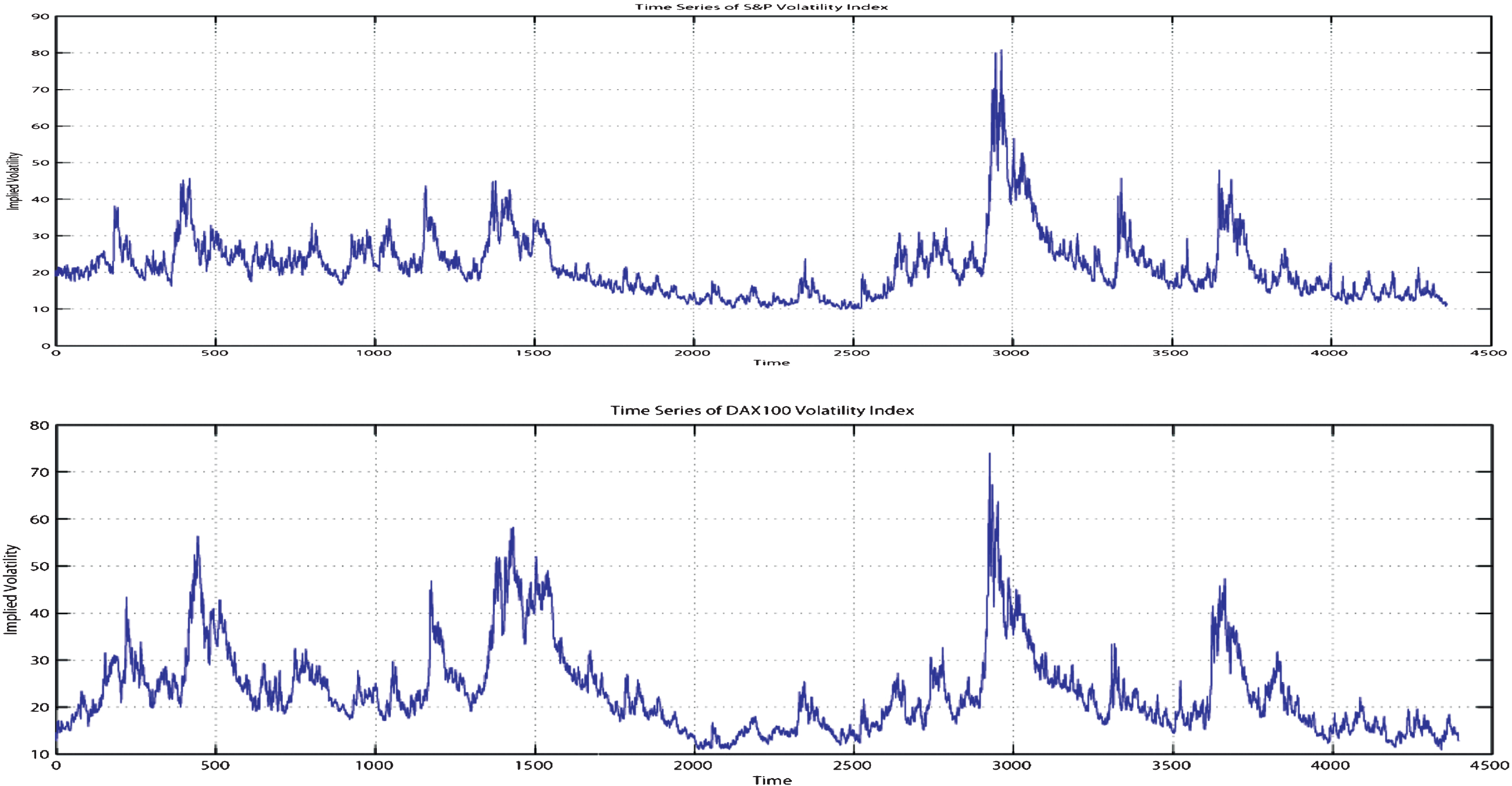
These figures present the time series of daily implied volatility for VIX (the top panel) and VDAX (the bottom panel) indices during the period 1997– 2014. The data sets show roughly the same behaviour during the time frame.This can be due to the effect of the global economic situation on the big markets. For instance, it can be observed that during the period of Subprime Lending Crisis, followed by the Global Financial Crisis (2007– 2009), the two markets exhibit a high level of volatility with a very similar pattern.

3.1 Support-reduction and local optimisation

The M-estimator is defined as the minimiser of a random criterion function over the parameter set. In parametric models, estimates can often be computed explicitly or approximated using some numerical technique for solving (low dimensional) convex unconstrained optimisation problems. Nevertheless, in our non-parametric case, we face a high dimensional constrained optimisation problem. Apart from the classic expectation maximisation of Dempster et al. (1977), there are a number of recent innovations in optimisation in the field of statistics. Here, we use the support-reduction (SR) algorithm, introduced in Groeneboom and Wellner (1992) and further developed in Groeneboom and Wellner (1992), Groeneboom et al. (2001) and Groeneboom et al. (2008). A version of this algorithm, known as the iterative convex minorant algorithm, was also used in Jongbloed et al. (2005) for the numerical approximation of the CME introduced in Section 2.1. However, the method of Groeneboom et al. (2008) (which is used in this paper) provides faster convergence, when computing non-parametric M-estimators in mixture models. Within the optimisation theory, the SR algorithm can be classified as a specific instance of an active set method. Within the field of statistical computing, the algorithm fits in the class of vertex direction algorithms. An algorithm, related to our support reduction algorithm, can be found in Meyer (1997), which led to the idea of the iterative spline algorithm for convex regression, as described in Groeneboom et al. (2001).

The algorithm discussed here is based on isotonic regression techniques as can be found in Härdle (1989). It is mostly used to compute shape-restricted estimators of distribution functions in semiparametric models. We apply the algorithm to compute M-estimators in mixture models, using unconstrained optimisations iteratively. It is to be noted that in each step the algorithm adds one support knot among several possible support knots to the existing iterate, resulting in a sparse next iteration. These reduced knots causes a low-dimensional unlimited optimisation problem during the next iteration. A fundamental advantage of this method is that in problems where the solution is a sparse mixture, the model can be handled well, due to the speed at which the low-dimensional optimisations are performed.

We seek to find an approximate solution for ${\overset{ˇ}{k}}_{n}$ , numerically and characterised by variational inequalities. The existence of a unique maximiser over the cone K_Θ is proven in Groeneboom et al. (2008), Lemma 1. Most importantly, they showed that ${\overset{ˇ}{k}}_{n}$ minimises Γ_n ∘ L (k) in (2.7) iff

$[D_{{\overset{ˇ}{k}}_{n}} (Γ_{n} \circ L)] (u_{θ_{j}}) {\begin{matrix} \geq 0 & \forall j \in {1, . . ., N}, \\ = 0 & \forall j \in J, \end{matrix}$ (3.8) where J : = {j ∈ {1, . . . , N} |α_j > 0} refers to the set of positive α-weights, and [D_aΦ] (b) is a directional derivative function from the right D_aΦ in the direction of a defined by $\begin{matrix} [D_{a} (Φ)] (b) : = lim_{ɛ \to 0} \frac{[Φ] (b + ɛ a) - [Φ] (b)}{ɛ} . \end{matrix}$

Note that whenever (Φ) (b)< ∞, convexity of Φ guarantees the existence of [D_a (Φ)] (b). Using straight forward, but tedious, calculations we can show $\begin{matrix} [D_{{\overset{ˇ}{k}}_{n}} (Γ_{n} \circ L)] (u_{θ_{j}}) = 2 〈 L u_{θ} - {\tilde{g}}_{n}, L {\overset{ˇ}{k}}_{n} 〉_{w} . \end{matrix}$

With a slight abuse of notations, let k^J from the cone K_Θ be the current iterate from each iteration. Then suppose k^J = ∑_j∈Jα_ju_{θ
_j}.

The optimisation algorithm in Groeneboom et al. (2008) prescribes to evaluate the optimality of k^J (3.8). If k^J is not optimal, then there exist an i ∈ {1, . . . , N} ∖ J with a negative directional derivative, which means u_{θ
_i} provides a direction of descent for the objective function. Therefore, our initial aim is to determine the set of grids with negative directional derivatives, all of which are non-optimal and provide a direction of descent. Then using a search algorithm, we pick a direction of descent and find a new iterate. In this stage, we must recalculate the optimal weights, using the standard least square technique. For doing so, we differentiate the objective functions with respect to α_j (j ∈ {1, . . . , m}) and set them to zero. This gives the following system

$〈 z_{θ_{i}}, z_{θ_{j}} 〉_{w} \underline{α} = 〈 z_{θ_{i}}, {\tilde{g}}_{n} 〉_{w}, i, j = 1, . . ., m,$ (3.9)

Equation (3.9) is easily proved by showing that the left-hand-side is symmetric and non-singular. This is briefly as follows.

Let A : = 〈z_{θ
_i}, z_{θ
_j}〉_w and ${\underline{α}}_{j}$ denote the j-th the column of A. We aim to show that if $\sum_{i = 1}^{m} = h_{i} {\underline{α}}_{i} = \underline{0}$ then all $h_{j} \in ℝ, j \in {1, \dots m}$ are zero. Now, $\sum_{k = 1}^{m} h_{k} w_{θ_{k}} (t) = 0$ for all t ∈ S, where $w_{θ} (t) = t \frac{d}{dt} z_{θ} (t) = cos (θ t) - 1 + i sin (θ t)$ .

Then also, $\begin{matrix} \frac{d^{p}}{{dt}^{p}} \sum_{k = 1}^{m} h_{k} w_{θ_{k}} (t) |_{t = 0} \\ = \sum_{k = 1}^{m} h_{k} (i θ_{k})^{p} = 0, p = 1, \dots, m . \end{matrix}$

Rewriting this in a linear system we find that $(\begin{matrix} i θ_{1} & i θ_{2} & \dots & i θ_{m} \\ - θ_{1}^{2} & - θ_{2}^{2} & \dots & - θ_{m}^{2} \\ ⋮ & ⋮ & ⋱ & ⋮ \\ (i θ_{1})^{m} & (i θ_{2})^{m} & \dots & (i θ_{m})^{m} \end{matrix}) (\begin{matrix} h_{1} \\ h_{2} \\ ⋮ \\ h_{m} \end{matrix}) = (\begin{matrix} 0 \\ 0 \\ ⋮ \\ 0 \end{matrix}) .$

Since the matrix in this display is a generalised Vandermonde matrix, its determinant is unequal to zero. Thus, h₁ = h₂ = ⋯ = h_m = 0.

Finally, we evaluate the new iterate by (3.8) for optimality, and repeat the process until the optimal solution is found.

Theorem 1 in Groeneboom et al. (2008) gives conditions to guarantee that the sequence of iterates {k⁽ⁱ⁾} _n (generated by the support-reduction algorithm) indeed converges to the solution of our minimisation problem. Since these conditions are met in our case, we have $(Γ_{n} L) (k^{(i)}) ↓ (Γ_{n} L) ({\overset{ˇ}{k}}_{n}), i \to \infty$

The support-reduction algorithm is summarised as follows

Step 1. In the current iterate, add a basis function u_θ for Γ_nL. Due to the linearity condition of L,

$\begin{matrix} [Γ_{n} L] (k + ɛ u_{θ}) - [Γ_{n} L] (k) \\ = ɛ c_{1} (θ, k) + \frac{1}{2} ɛ^{2} c_{2} (θ), \end{matrix}$ (3.10)

where $\begin{matrix} c_{1} (θ, k) & = & 2 〈 Lk - {\tilde{g}}_{n}, {Lu}_{θ} 〉_{w}, and \\ c_{2} (θ) & = & 2 | | {Lu}_{θ} | |_{w}^{2} . \end{matrix}$

Step 2. To obtain a direction of descent, pick a θ ∈ Θ for which c₁ (θ, k) <0. Since, (3.10) is quadratic in ɛ, it can be minimised explicitly, which yields

$\begin{matrix} \hat{θ} & = & \underset{{θ \in Θ : c_{1} (θ, k) < 0}}{arg min} - \frac{c_{1} (θ, k)^{2}}{2 c_{2} (θ)} \\ = & \underset{θ \in Θ}{arg min} \frac{c_{1} (θ, k)}{\sqrt{c_{2} (θ)}} . \end{matrix}$ (3.11)

Step 3. Compute optimal weights, for the support points. This is a standard least-squares problem which is solved by the normal equations.

We implement the Divide and Conquer (D&C) algorithm to search for the solution. In this algorithm, a successful join of points is determined when the new solution decreases the objective function and is not outside of K_Θ. Throughout the optimisation process, we may find solutions that contain support points in too close vicinity of each other. This is because the grids are not continuous. To prevent such situation we locally optimise the support by scanning for closely located points. If we found such support points, we determine a convex combination of them that minimises Γ_n ∘ L (k). This may have a smoothing effect that does not interfere with the convergence condition specified in Groeneboom et al. (2008). Additionally, the extra step can reduce the convergence speed dramatically; therefore, we will only implement the replacement when we find two points with two new directions of descend, that cause the algorithm zigzag between them.

Another issue that might arise is that the solution α_i may generate a measure ∑α_iu_{θ
_i}, not necessarily belonging to ℛ⁺ as α_i might be negative for some i. If this function happens to belong to ℛ⁺, it is a new iterate. Otherwise, one travels as far as possible along the line segment connecting the current iterate with this infeasible measure. A remedy for this problem is offered in Groeneboom et al. (2008), which we implement in our algorithm as part of Step 2. For this purpose, we use a sequence of unrestricted minimisations and support-reduction, to obtain a new subset of support-points that minimises Γ_n ∘ L (k).

Finally, in relation to the computational efficiency the support-reduction estimation has a very low run time. Even though the calculation of matrix c₂ (θ) needs a long time (in fact it depends on the total number of mesh grids), the algorithm works highly efficiently, once it is initialised, the determination of the vector is fast.

3.2 In-sample estimation

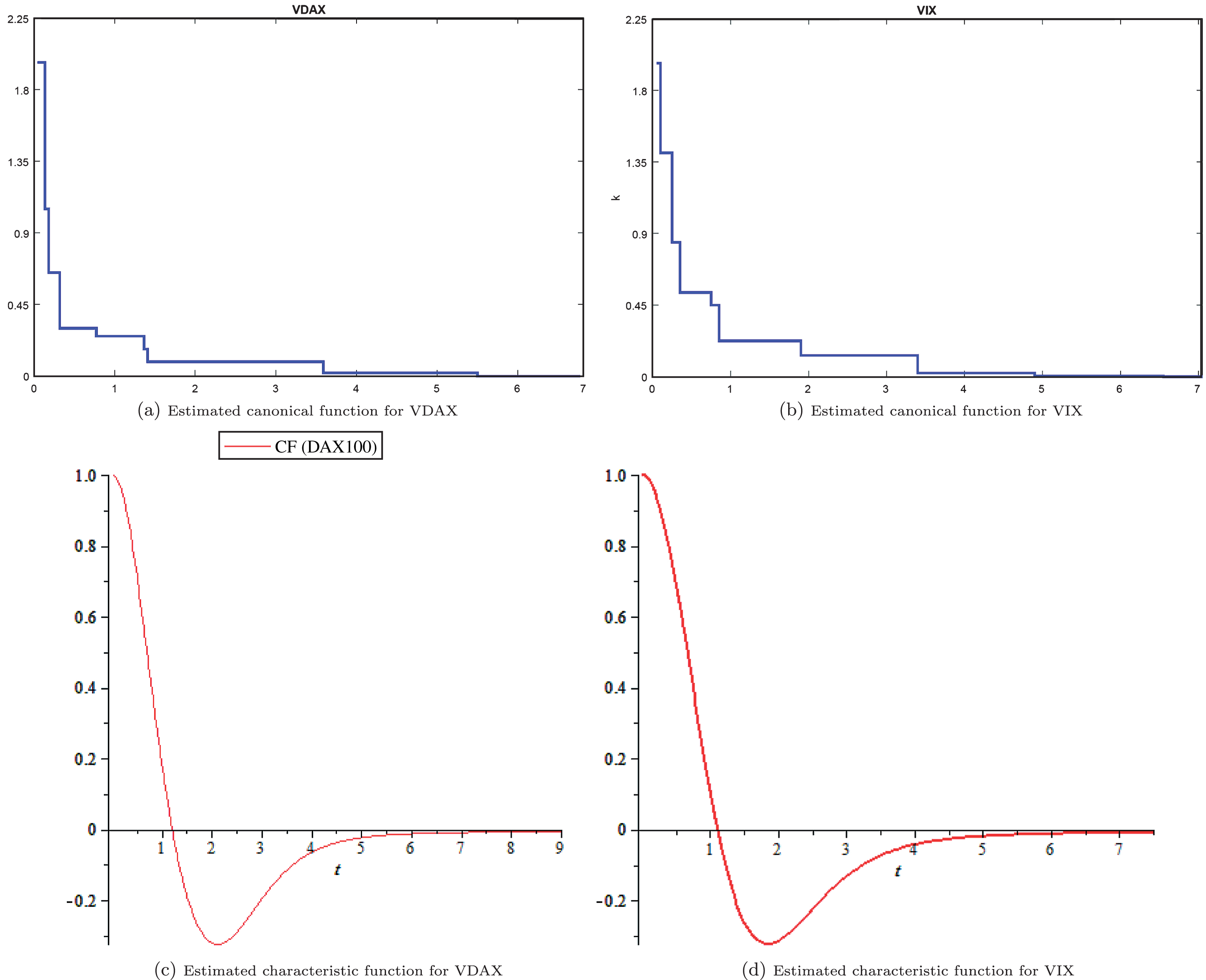
In this section, we approximate the canonical functions for VDAX and VIX, using the cumulant M-estimator. Further, we approximate the intensity parameter λ for the implied volatility of both indices. Table 1 presents the results for the support-reduction algorithm applied to the volatility data set. Additionally, Fig. 2 plot $\tilde{ψ} (t)$ for each of the volatility indices.

Fig.2

These figures exhibit the plots for the estimated canonical functions and characteristic functions for both VIX and VDAX. The shape of the characteristic functions remind us of log-normal distribution, therefore, we test the hypothesis that whether the data sets were drawn from log-normal distributions. The results are provided in Table 1.

Table 1

This table reports M-estimators estimates and corresponding weights and lambda estimation for the two different data sets. The algorithm ran until the directional derivative on all grid points was above 10^-15

Volatility Index	Cumulant M-estimators estimates				λ estimation
	α ₁	θ ₁	α ₂	θ ₂
VIX	1.9525	0.75	0.0483	1.10	0.6317
VDAX	2.1048	0.60	0.0540	3.00	0.7287

Next, we want to obtain the stationary distribution function f_n using fast Fourier transform. Note that $\begin{matrix} \tilde{ψ} (t) & = & exp (\int_{0}^{\infty} (e^{ity} - 1) \frac{\tilde{k} (y)}{y} dy), \\ = & exp (\sum_{j = 1}^{M} α_{j} z_{θ_{j}} (t)), \end{matrix}$ thus, $\begin{matrix} \tilde{f} (y) = \frac{1}{2 π} \int_{- \infty}^{\infty} e^{- ity + \sum α_{j} z_{θ_{j}} (t)} dt . \end{matrix}$

The characteristic function of a self-decomposable distribution does not need to be integrable. Such condition means that there is no guarantee that we can calculate the Fourier transform analytically. Here, we use an alternative method based on Schorr (1975), where we numerically approximate the Fourier transform. We only present the results for the numerical approximation, without the proof. Interested readers may refer to Schorr (1975) for the detailed calculations of similar examples. $\begin{matrix} f (y) = \sum_{κ = - \infty}^{+ \infty} a_{κ} exp (i κ wy), \end{matrix}$ where the parameters are defined as follow: $\begin{matrix} a_{k} & = & \frac{w}{2 π} \int_{- \infty}^{+ \infty} f (u) exp (- i κ wu) du \\ = & \frac{w}{2 π} \tilde{ψ} (- κ w) . \end{matrix}$ Here, $w = \frac{2 π}{T}$ , T = T₊ - T_-, where $\begin{matrix} T_{+} = (- 2 ln (ɛ_{+}))^{\frac{1}{2}} σ, \\ T_{-} = (- 2 ln (ɛ_{-}))^{\frac{1}{2}} σ, \end{matrix}$ where σ is the standard deviation of the data, so Fourier approximation follows

$\begin{matrix} \tilde{f} (y) & = & \sum_{κ = - \infty}^{\infty} T^{- 1} exp (\sum_{j = 1}^{M} α_{j} \\ \int_{0}^{jhw κ} \frac{e^{- iz} - 1}{z} dz + i κ wy) . \end{matrix}$ (3.12) Schorr (1975) shows that $\tilde{f} (y)$ is well defined.

We consider 60 grid points for the numerical approximation with lags of 0.05; therefore, we will have 60 basis functions. Moreover, for estimation of density functions based on the Fourier transform, T is considered to be 12 and κ takes values from -150 to 150. This interval is sufficiently large enough to obtain a reasonably accurate approximation.

Next, using the MLE method discussed in the previous section, we estimated the intensity parameters, λ, which are also reported in Table 1, then, in Fig. 3 we plot the non-parametrically estimated distributions for both indices, overlaying the histogram of the datasets.

Fig.3

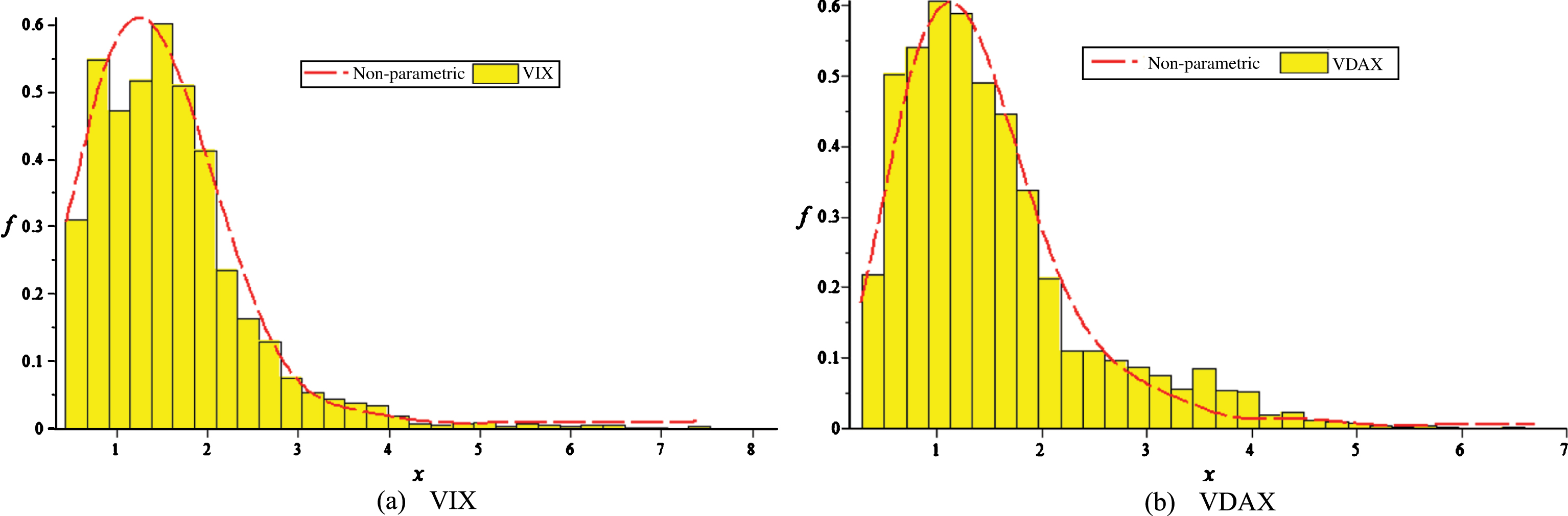
These figures exhibit the plots for the non-parametrically estimated density functions for VIX and VDAX, overlaying the histogram of the datasets.

Fig.4

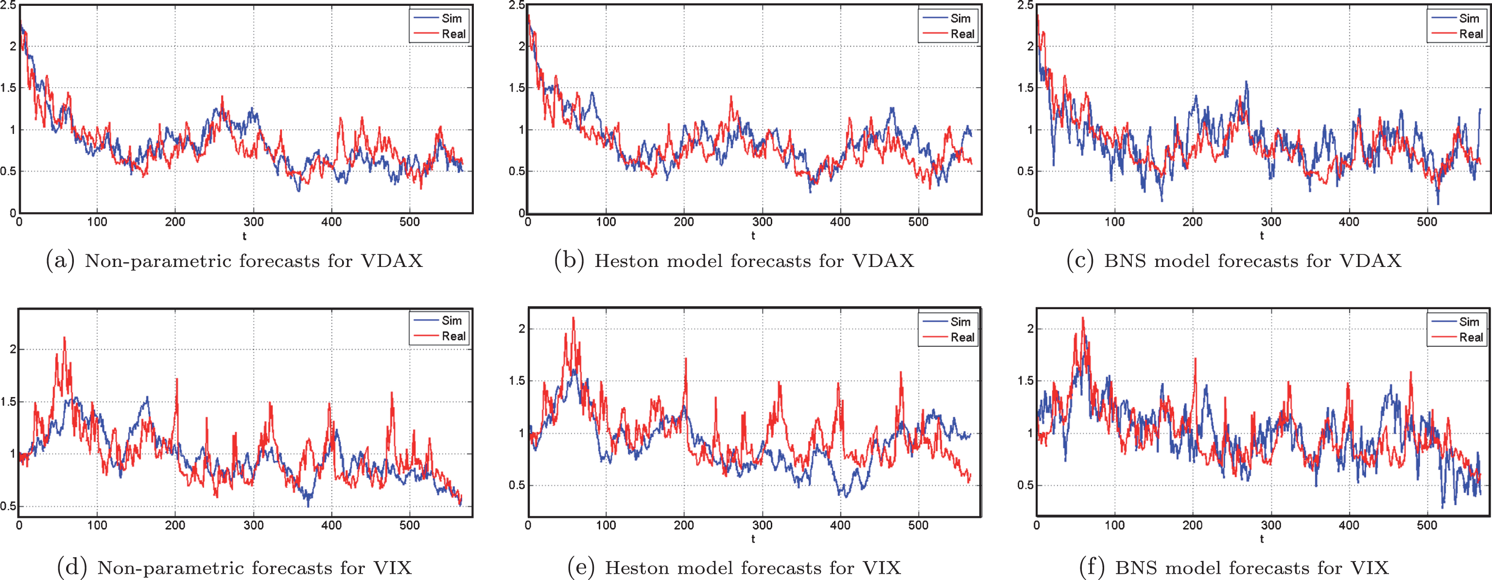
These figures present a comparison between different stochastic volatility models (i.e. non-parametric, Heston and BNS models) and their forecasting abilities. Out-of-sample simulated paths are indicated by blue lines and the times series (real) of daily implied volatility for the same time periods are indicated by red lines.

In order to compare the performance of our non-parametric model with some conventional parametric cases; namely, log-normal, Inverse Gaussian, Burr, and Gamma. At the beginning of the paper we argued that the flexibility of the non-parametric framework is a considerable advantage of our approach to model implied volatility, compared to the parametric cases. Here, we are interested to compare the statistical power of our model with the above mentioned parametric models. A fundamental issue in statistical analysis is testing the fit of a particular probability model to a set of observed data. A simulation approximation to the null distribution of the test provides a convenient and powerful means of testing model fit. Tu (2006) proposed a new Monte Carlo-based methodology to construct this type of approximation when the model is semi-structured. They showed that when there are no nuisance parameters to be estimated, the non-parametric Monte Carlo test can exactly maintain the significance level and when nuisance parameters exist, this method can allow the test to asymptotically maintain the level.

Generating random values from the estimated density function (3.12) requires some effort, since the quantile function is not available in closed form and the inversion method is, therefore, not possible. As an alternative, since $\tilde{f} (y)$ is unimodal, we consider the acceptance-rejection method, which is a type of Monte Carlo method based on the observation that to sample a random variable one can sample uniformly from the region under the graph of its density function. Acceptance-rejection method assumes the existence of a density g and the knowledge of a constant c such that $\tilde{f} (y) \leq cg (y), \forall y$ . Therefore, in order to apply the algorithm, one needs to be able to determine a suitable constant c. Besides, it is necessary to specify an appropriate random variable with density g, such that cdf G easily invertible and g has to dominate $\tilde{f}$ .

The basic idea is to search for a density function g, from which we already have an efficient algorithm to generate from, but also such that the function g is “close” to $\tilde{f}$ . Therefore, the ratio $\tilde{f} (y) / g (y)$ is bounded by c, that is

$sup {\tilde{f} (y) / g (y)} \leq c .$ (3.13)

As in Devroye (1986), the algorithm for generating random variables distributed as $\tilde{f}$ is

Step 1. Determine g and its parameters such that it dominates $\tilde{f}$ . The parameters of g are set such that the first four moments of g are as close as possible to the first four moments of $\tilde{f}$ .

Step 2. Use (3.13) to compute c graphically or numerically.

Step 3. Generate a r.v. X distributed as g.

Step 4. Generate a uniform r.v. U, independent from X.

Step 5. If $U \leq \frac{\tilde{f} (X)}{c . g (X)}$ , then set Y = X (accept), otherwise, go back to Step 3.

For the density functions of both of the datasets, we consider a wide range of candidates for g and their parameters specifications, such that the dominance condition is met. Choosing the most appropriate g is a heuristic process, for which our best guide is the constant c. It can be mathematically presented that the acceptance rate is 1/c, then the expected number of iterations of the algorithm required must be c (cf. Sigman (2007)). If this is not met, we must try a different g.

We found that for simulating (3.12), log-normal distribution is a suitable choice for g. Simulating from this distribution is relatively simple and fast, which is especially important since, in order for the $\tilde{f} (y)$ to be dominated, the factor c needs to grow with the kurtosis. As a result, the number of rejections also increases and, if the algorithm to generate from the dominating density is not sufficiently fast, computation becomes slow. Table 2 reports the parameter specifications of the log-normal distributions used for each data set, as well as the acceptance rate and the boundary constant, c. We can see that in all cases the inverse of the acceptance rate is very close to c, which verifies the appropriateness of choosing the log-normal distribution. We thus have two Kolmogorov-Smirnov (KS) tests and two Anderson-Darling (AD) tests, applied to the simulated distributions. The KS test is based on the maximum distance between the cumulated probability functions of the simulated density and the sample, whereas the AD test gives more weight to the tails than does the K-S test. In all four scenarios we accept the null hypothesis at the significance levelof 0.05.

Table 2

This table reports the parametric specifications of the log-normal distributions used as g for each dataset, as well as the acceptance rate and the boundary constant, c. On the right-hand side, the table reports the Kolmogorov-Smirnov and Anderson-Darling statistics and p-values from the respective goodness-of-fit tests

Sample	g ∼ ln 𝒩 (μ, σ²)		Accept -rate	c	Kolmogorov–Smirnov		Anderson–Darling
	μ	σ			Statistic (D)	p-value	Statistic (D)	p-value
VIX	0.464	0.3616	1.05	0.8936	0.0512	0.5799	0.5948	0.6618
VDAX	0.650	0.2159	1.04	0.8608	0.0499	0.6502	0.6090	0.6384

Next, we compare if our non-parametric estimation of the density better fits the data better than some conventional parametric cases. Table 3 reports this comparison using log-normal, Inverse Gaussian, Burr, and Gamma distributions. At a significant level of 0.05, we can clearly reject the null hypothesis that our samples (both VIX and VDAX) are from Inverse Gaussian, Burr or Gamma distributions. Nevertheless, the log-normal appears to be a contester for our model. For both VIX and VDAX we can accept the null hypothesis that our sample is from a log-normal distribution. In terms of the KS-test, the log-normal distribution has even slightly out performed our model, evident from their p-values. However, the p-values of the AD tests suggests that our non-parametric model might out perform the log-normal distribution in modelling the tail behaviours. The results are too close to conclusively identify the better model, however, due to the general advantageous of non-parametric approaches (discussed in Section 1), our method is still preferred.

Table 3

This table reports the Kolmogorov-Smirnov and Anderson-Darling statistics and p-values from the goodness-of-fit tests of different distributions; namely, log-normal, Inverse Gaussian, Burr, and Gamma, as well as our non-parametrically estimated density function

Sample	Distribution	Parameter estimation	Kolmogorov–Smirnov		Anderson–Darling
			Statistic (D)	p-value	Statistic (D)	p-value
VIX	Nonparametric	–	–	–	0.0512	0.5799	0.5948	0.6618
	Log-Normal	μ = 0.3616	σ = 0.4920	γ = 0.0006	0.0491	0.6131	0.8876	0.4215
	Inv-Gaussian	λ = 5.7473	μ = 1.6218	–	0.2423	0.0001	6.8270	0.0000
	Burr	k = 1.2909	α = 3.2758	β = 1.6159	0.2364	0.0002	5.8405	0.0000
	Gamma	α = 3.5438	β = 0.4577	γ = 0.0000	0.4789	0.0000	8.5550	0.0000
VDAX	Nonparametric	–	–	–	0.0499	0.6502	0.6090	0.6384
	Log-Normal	μ = 0.2159	σ = 0.5900	γ = 0.0549	0.0470	0.7248	0.7600	0.5741
	Inv-Gaussian	λ = 4.3982	μ = 1.5270	–	0.1225	0.0227	2.6827	0.0000
	Burr	k = 1.0953	α = 3.0051	β = 1.3652	0.1227	0.0213	3.1623	0.0000
	Gamma	α = 1.9915	β = 0.6253	γ = 0.2817	0.3614	0.0019	4.5020	0.0000

3.3 Out-of-sample forecasts

Model selection depends not only on the goodness-of-fit of a model to the data, but also on the objective of the analysis. For forecasting, a model that is best in the in-sample fitting does not necessarily provide more accurate forecasts. Thus, many people use the performance of out-of-sample forecasts to aid the selection of a statistical model.

Statistical tests of a model’s forecast performance are commonly conducted by splitting a given data set into an in-sample period, used for initial parameter estimation and model selection, and an out-of-sample period, used to evaluate forecast performance. Empirical evidence based on out-of-sample forecast performance is generally considered more trustworthy than evidence based on in-sample performance which can be more sensitive to outliers and data mining (White (2000)). Out-of-sample forecasts also better reflect the information available to the forecaster in “real time”. This has led many researchers to regard out-of-sample performance as the “ultimate test of a forecasting model” (Stock and Watson (2007)).

We divide the data for both VIX and VDAX into two sub-periods, namely, the estimation sub-sample which is the first period, and the forecasting sub-sample which is the remainder of the data set. Given T data points, say x₁, …, x_T, we divide the data as {x₁, …, x_n} and {x_n+1, …, x_T}, where n is the initial forecast origin.

Suppose, three competing models: A) the non-parametric model in the current work B) the Heston’s stochastic volatility model (Heston (1993)) and C) the BNS pure jump stochastic volatility model (Barndorff-Nielsen et al., (2002))) with Gamma marginal distribution as in Griffin and Steel (2006).

Let h be the forecast horizon, i.e. we are interested in 1-step to h-step ahead forecasts. The out-of-sample forecasting evaluation works as follows:

Let m = n be the initial forecast origin. Fit models A, B and C. Note that for the non-parametric case, we need to repeat the support-reduction algorithm for the new window. For brevity, we do not discuss the calibration of models B and C. Interested readers may refer to Schorr (1975) and Griffin and Steel (2006).

For each model, conduct a simulation experiment and calculate the 1-step to h-step ahead forecasts, denoted by ${\hat{x}}_{m} (1), \dots, {\hat{x}}_{m} (h)$ . Note that the for model A, it is required to simulate a sample path for the subordinator Z, which is a finite activity process. For simulation of Z, we use the concept of series representations for general Lévy measures introduced in Rosiński (2001), where the simulated mean measures are obtained by the “acceptance-rejection” method discussed in Section 3.

Advance the forecast origin by 1, i.e. m = m + 1, and go to Step 1.

The iteration stops when the forecast origin is m = T.

In this way, we will have (T - n - 1) 1-step ahead forecast errors for each model, and (T - n - 2) 2-step ahead forecast errors for each model, and so on. For l-step ahead forecasts of the model, we then compute the following three functions in the models out-of-sample forecast performance evaluation. $\begin{matrix} MSE (l) & = & \frac{1}{T - l} \sum_{t = 1}^{T - l} {(x_{t + l}^{2} - {\hat{x}}_{t}^{2} (l))}^{2}, \\ R^{2} LOG (l) & = & \frac{1}{T - l} \sum_{t = 1}^{T - l} {(log (\frac{x_{t + l}^{2}}{{\hat{x}}_{t}^{2} (l)}))}^{2}, \\ PSE (l) & = & \frac{1}{T - l} \sum_{t = 1}^{T - l} {(\frac{x_{t + l}^{2} - {\hat{x}}_{t}^{2} (l)}{{\hat{x}}_{t}^{2} (l)})}^{2}, \end{matrix}$ where l = 1, 2, …, h. These three criteria were all suggested by Griliches et al. (1994). The Mean Square Error (MSE) is the average of the squared deviations of the forecast from the implied volatility. Hence, one large deviation is given a much higher weighting than a sum of small deviations even if the sum of the deviations is equal to the one time large deviation. When evaluating volatility forecasting performance this can seem quite illogical since in general one large deviation is not more troublesome than a sum of small deviations that sum up to the size of the large deviation. Moreover, single outliers will have a significant impact on the MSE criteria. The R²LOG still assigns higher weighting to large deviations but they are not as penalised as in the case of MSE. The Percentage Squared Errors (PSE) measures the average of the squared percentage deviation. The deviations are expressed as a percentage of the forecasted volatility. Hence, the PSE takes into account the fact that it is harder to be accurate, in an absolute sense, when estimating high variances and thus measures the relative error as a percentage to account for this.

For all the three loss functions a smaller value is preferred. Table 4 reports the average MSE, R²LOG, and PSE for the two compared parametric implied volatility models, as well as the proposed non-parametric model. The results, unequivocally, suggest that our non-parametric model provides a better out-of-sample fit (in terms of MSE, R²LOG, and PSE) in all cases for both VIX and VDAX.

Table 4
Average MSE, R²LOG, and PSE for the compared parametric implied volatility models (i.e. Heston model and BNS model with Gamma marginal distribution) and the proposed non parametric model

MSE R2LOG PSE

VIX Non-parametric 0.0456 0.1713 0.0437

Heston 0.0635 0.2692 0.2736

BNS 0.0590 0.3435 0.2735

VDAX Non-parametric 0.0402 0.4410 0.2898

Heston 0.0476 0.3174 0.2774

BNS 0.0572 0.3967 0.4482

		MSE	R2LOG	PSE
VIX	Non-parametric	0.0456	0.1713	0.0437
	Heston	0.0635	0.2692	0.2736
	BNS	0.0590	0.3435	0.2735
VDAX	Non-parametric	0.0402	0.4410	0.2898
	Heston	0.0476	0.3174	0.2774
	BNS	0.0572	0.3967	0.4482

4 Conclusion

We developed an intuitive non-parametric framework to estimate stochastic implied volatility. We proposed that implied volatility can be modelled by a Lévy driven OU process, the Lévy measure of which is hidden to the market. Using discrete-time observation, we provide a robust non-parametric estimation technique for estimating the Lévy density of the invariant law of a stationary OU process that is driven by a subordinator. In contrast to other non-parametric estimators (such as kernel estimators), our estimator is guaranteed to be of the correct type. We implement this method with the aid of a support-reduction algorithm, which is an efficient iterative unconstrained optimisation method.

We present a comprehensive empirical analysis, using discretely observed data from two implied volatility indices, VIX and VDAX. Further, we analyse the goodness-of-fit of our estimated distribution by simulating it with the acceptance-rejection method. We have conducted the KS test and the AD test for the non-parametrically estimated density functions of VIX and VDAX data, as well as some conventional parametric cases for the purpose of comparison. We concluded that except for the case of log-normal distribution, our method clearly outperformed other methods. We also present an out-of-sample test to compare the forecasting power of our method with other parametric models; namely, Heston and BNS models. Our non-parametric method outperformed in every case, using different metrics.

This paper has extended an efficient and accurate statistical model for implied stochastic volatilities. Further research may investigate the application of this model in pricing derivatives, using the analytically tractable structure of (2.1).

References

Ait-Sahalia

, 1996. Nonparametric pricing of interest rate derivative securities, Econometrica 64, 527–560.

Applebaum

, 2009. Le´vy processes and stochastic calculus, Cambridge university press.

Bandi

F.M.

, Renò

, 2011. Nonparametric stochastic volatility, Available at SSRN 1158438.

Barndorff-Nielsen

O.E.

, Leonenko

, 2005. Spectral properties of uperpositions of ornstein-uhlenbeck type processes, Method¬ology and Computing in Applied Probability 7(3), 335–352.

Barndorff-Nielsen

O.E.

, Nicolato

, Shephard

2002. Some recent developments in stochastic volatility modelling, Quan¬titative Finance 2(1), 11–23.

Barndorff-Nielsen

, Shephard

, 2001. Non-gaussian ornstein–uhlenbeck-based models and some of their uses in financial economics, Journal of the Royal Statistical Society: Series B (Statistical Methodology) 63(2), 167–241.

Birru

, Figlewski

, 2010. The impact of the federal reserve’s interest rate target announcement on stock prices: A closer look at how the market impounds new information, Stern School of Business, New York University.

Carr

, Geman

, Madan

D.B.

, Yor

, 2003. Stochastic volatil-ity for le´vy processes, Mathe-matical Finance 13(3), 345–382.

Chen

, Mohan

, Steiner

, 1999. Discount rate changes, stock market returns, volatility, and trading volume: Evidence from intraday data and implications for market efficiency, Jour¬nal of Banking & Finance 23(6), 897–924.

10.

Cont

, da Fonseca

, 2002. Deformation of implied volatility surfaces: An empirical analysis, Springer.

11.

Davydov

, 1973. Mixing conditions for Markov chains, Teoriya Veroyatnostei i ee Primeneniya 18(2), 321–338.

12.

Dempster

, Laird

, Rubin

, 1977. Maximum likelihood from incomplete data via the emalgorithm, Journal of the Royal Statistical Society 39(1), 1–38.

13.

Devroye

, 1986. Sample-based non-uniform random variate generation, in Proceedings of the 18th conference on Winter simulation, ACM, pp. 260–265.

14.

Ehrmann

, Fratzscher

, 2005. Exchange rates and fundamen¬tals: New evidence from real-time data, Journal of International Money and Finance 24(2), 317–341.

15.

Gander

M.P.

, Stephens

D.A.

, 2007. Stochastic volatility mod¬elling in continuous time with general marginal distributions: Inference, prediction and model selection, Journal of Statistical Planning and Inference 137(10), 3068–3081.

16.

Getoor

, 1975. Markov processes: Ray processes and right pro¬cesses, Springer.

17.

Griffin

J.E.

, Steel

M.F.

, 2006. Inference with non-gaussian ornstein–uhlenbeck processes for stochastic volatility, Journal of Econometrics 134(2), 605–644.

18.

Griliches

, Engle

R.F.

, Intriligator

M.D.

, 1994. Handbook of econometrics, Elsevier.

19.

Groeneboom

, Jongbloed

, Wellner

, 2001. Estimation of a convex function: Characterizations and asymptotic theory, Annals of Statistics, pp. 1653–1698.

20.

Groeneboom

, Jongbloed

, Wellner

, 2008. The support reduction algorithm for computing non-parametric function estimates in mixture models, Scandinavian Journal of Statistics 35(3), 385–399.

21.

Groeneboom

, Wellner

, 1992. Information bounds and non-parametric maximum likelihood estimation, 19, Springer.

22.

Ha¨rdle

, 1989. Robertson, t., wright, ft and rl dykstra: Order restricted statistical inference, Statistical Papers 30(1), 316–316.

23.

Heston

S.L.

, 1993. A closed-form solution for options with stochastic volatility with applications to bond and currency options, Review of Financial Studies 6(2), 327–343.

24.

Hull

, White

, 1987. The pricing of options on assets with stochastic volatilities, The Journal of Finance 42(2), 281–300.

25.

Jongbloed

, 1998. The iterative convex minorant algorithm for nonparametric estimation, Journal of Computational and Graphical Statistics 7(3), 310–321.

26.

Jongbloed

, Van Der Meulen

, Van Der Vaart

, 2005. Nonparametric inference for le´vydriven Ornstein-Uhlenbeck processes, Bernoulli 11(5), 759–791.

27.

Krengel

, Brunel

, 1985. Ergodic theorems, 59, Cam¬bridge Univ Press.

28.

, Wells

M.T.

, Cindy

L.Y.

, 2008. A bayesian analysis of return dynamics with le´vy jumps, Review of Financial Studies 21(5), 2345–2378.

29.

, Li

, Han

, 2015. Stochastic lattice models for valua¬tion of volatility options, Economic Modelling 47, 93–104.

30.

Masuda

, 2004. On multidimensional ornstein-uhlenbeck pro¬cesses driven by a general le´vy process, Bernoulli 10(1), 97–120.

31.

Meyer

M.C.

, 1997. Shape restricted inference with applications to nonparametric regression, smooth nonparametric function estimation, and density estimation, PhD thesis, Department of Statistics, University of Michigan.

32.

Mikhailov

, No¨gel

, 2004. Hestons stochastic volatility model: Implementation, calibration and some extensions, John Wiley and Sons.

33.

Nielsen

, Shephard

, 2003. Likelihood analysis of a first-order autoregressive model with exponential innovations, Journal of Time Series Analysis 24(3), 337–344.

34.

Roberts

G.O.

, Papaspiliopoulos

, Dellaportas

, 2004. Bayesian inference for non-gaussian ornstein–uhlenbeck stochastic volatility processes, Journal of the Royal Statistical Society: Series B (Statistical Methodology) 66(2), 369–393.

35.

Rosi_nski

, 2001. Series representations of le´vy processes from the perspective of point processes, in Le´vy processes, Springer, pp. 401–415.

36.

Sato

, 1999. Le´vy processes and infinitely divisible distribu¬tions, Cambridge university press.

37.

Schorr

, 1975. Numerical inversion of a class of characteristic functions, BIT Numerical Mathematics 15(1), 94–102.

38.

Shiga

, 1990. A recurrence criterion for markov processes of ornstein-uhlenbeck type, Probability Theory and Related Fields 85(4), 425–447.

39.

Sigman

, 2007. Acceptance-Rejection Method, Columbia Uni¬versity.

40.

Soulier

, 1998. Nonparametric estimation of the diffusion coefficient of a diffusion process, Stochastic Analysis and Applications 16(1), 185.

41.

Stock

J.H.

, Watson

M.W.

, 2007. Introduction to econometrics, 104, Addison Wesley Boston.

42.

Todorov

, 2011. Econometric analysis of jump-driven stochastic volatility models, Journal of Econo-metrics 160(1), 12–21.

43.

Todorov

, Qin

, 2017. Nonparametric implied levy densities, Working Paper.

44.

, 2006. Nonparametric monte-carlo tests and their applica¬tions, Biometrics 62(3), 950–951.

45.

White

, 2000. A reality check for data snooping, Econometrica, pp. 1097–1126.

46.

Zhang

, Xu

, 2014. Optimal stopping time with stochastic volatility, Economic Modelling 41, 319–328.

A non-parametric inference for implied volatility governed by a Lévy-driven Ornstein–Uhlenbeck process

Abstract

Keywords

1 Introduction

1.1 Background

2 Theoretical framwork

3 Estimation and empirical results

References