Modeling the financial market with labyrinth chaos

Abstract

In the present study, a deterministic model is introduced to explain the stylized facts of financial data. The adaptation introduced by the labyrinth chaos model can reproduce phenomena such as heavy tails observed in financial returns, volatility clustering and jumps. The model is based on the assumption that many unstable stationary states arise from the interaction or feedback between financial prices. Model tests are performed, and the results show that the model generates series that reject a normal distribution of the returns and which can be represented by the GARCH model. An analysis applying symbolic dynamics shows similar behaviors in a system with three stock indices, three currency relations and three prices generated by the introduced model. We observe sequences that have not been produced by any of the three systems, suggesting that in a three-dimensional space, the paths traveled by the real series and those of the model may not be completely random.

Keywords

Financial markets stylized facts volatility clustering chaos financial time series brownian motion 0000-0002-8618-7456 C02;C60;G11;G12;G14

1 Introduction

In the present study, we introduce a deterministic model that attempts to explain stylized facts, a series of phenomena observed in the financial markets. The most common and known statistical regularities include heavy tails, volatility clustering, non-normal returns and jumps. Considering the extensive literature and to simplify and classify the present exposition, we classify studies on financial markets and stylized facts in two groups.

In the first group, we include the modern stochastic models applied in financial analysis, which are well accepted among economists and academics. Their developments are based on the Brownian process as a basic model, in which the financial variation of variables, such as stock prices, market indices or exchange rates, are represented as random processes. The discrete version of this model is the well-known random walk. Bachellier (1900) was the first to propose that stock prices and indices follow a Brownian process and Malkiel (1999) presented an excellent defense of the random walk model. This process is based on the efficient markets hypothesis proposed by Fama (1965). According to this hypothesis, stock prices already incorporate all the existing information and therefore, there is no way to predict the market. The main disadvantage of stochastic models is that randomness explains most of the evolution of a certain variable without clarifying the economic or financial causes behind the movements of that variable.

A second group of explanations is related with complex dynamical systems and, in particular, deterministic chaos. Complex dynamics is popular among mathematicians and physicists who in the last decades have been dedicated to studying economic phenomena. In this group, we found the research field known as econophysics, which uses methods that are applied in physics to the economy. Clearly, the application of physics to economics is not new, as the origin of many economic theories lie in physics explanations; however, there is a different approach. An introduction to econophysics can be found in Mantegna and Stanley (2000) and in Bouchaud and Potters (2003). According to this field, the phenomena observed in financial markets stem from complex interactions between economic agents that can be modeled not only by non-linear stochastic processes but also in deterministic form through complex dynamic systems, particularly those that arise from the theory of deterministic chaos. In this sense, Mandelbrot and Van Ness (1968) propose that prices follow a fractional Brownian motion and financial markets behave as fractals, while in Peters (1994; 1996) and Mandelbrot (1997), there is evidence of fractality in these markets. The theory of chaos stimulates interest because we can observe phenomena that are purely deterministic but appear to be random.

In fact, one of the aspects differentiating deterministic chaos from stochastic models is the subject of randomness. This issue remains one aspect of the philosophical and scientific debate. Notably, not even the example of flipping a coin is a random phenomenon, since knowing variables, such as the initial position of the coin, the force that is printed on it, the direction and force of the wind, among other initial conditions, would allow a prediction to be made regarding the trajectory and final position of the coin. However, our ignorance of all these variables allows us to consider the dynamics of flipping a coin as if they were random phenomena. Consider that the random number generators in statistical software are actually pseudorandom generators governed by highly complex dynamic systems. As mentioned, stochastic models use randomness to model uncertainty. However, in doing so, the main disadvantage is that part of the problem is left unexplained. The deterministic processes have the advantage of providing a possible explanation for the observed dynamics; however, the evidence for low level chaos remains weak, and it is therefore necessary to develop powerful statistical tests for determinism. Note that most of the statistical tests are based on assuming randomness in the null hypothesis, but it is more difficult to assume that determinism exists in a null hypothesis. This issue becomes more complex considering the large number of possible deterministic non-linear models.

Certain stylized facts and market failures have been observed that make the Brownian model mentioned above inappropriate for financial markets. Lo and MacKinlay (1998) use the variance ratio test and find that financial returns do not behave randomly. This has led scholars to seek explanations for the deviations that occur with respect to the model. Singal (2004) reviews all the anomalies found thus far. First, financial returns do not appear to follow a Gaussian distribution. That is, although they appear to behave randomly over time or have a very low autocorrelation, their empirical density function appears to have a higher probability in the tails than that which would have a normal distribution. This phenomenon is referred to as heavy tails or fat tails, see Fang and Lai (1997) for review of this information. This would mean that the empirical distribution of financial returns is leptokurtic, displaying a particularly sharper peak than that produced by a Gaussian distribution. Scholars have attempted to simulate this phenomenon using different density functions such as the t-Student, power-law or Pareto distributions, although they do not appear to completely reproduce this phenomenon. Additionally, there are no completely satisfactory explanations regarding this phenomenon; one explanation relates to another stylized fact that may cause it, volatility clustering, first discovered by Mandelbrot (1963). It is well known that volatility plays an important role in financial modeling as a measure of risk and is important in the modeling of financial derivatives, as seen in Hull (2006) and Black and Scholes (1973). Volatility clustering implies that there are periods of time for which volatility is higher and other periods for which the volatility of returns is lower, which forms two different clusters. This would show that there is some dependence within the dynamics of volatility; however, it is not possible to model this dependence with a classic Brownian process or to generate it with the traditional random walk. There are a series of models that attempt to reproduce this phenomenon based on the ARCH model proposed by Engle (1982). The ARCH model suggests that the variance of financial returns behaves as an autoregressive process. Although the model is very useful and appropriate for broad empirical application, for example, in the valuation of financial derivatives, it does not offer an explanation from the economic or financial point of view but rather attempts to simulate the observed behavior. Engle (2004) asserts that generalizations of the ARCH model have been proposed by many researchers, includingmodels such as the AARCH, APARCH, FIGARCH, FIEGARCH, STARCH, SWARCH, GJR-GARCH, TARCH, MARCH, NARCH, SNPARCH, SPARCH, SQGARCH, and CESGARCH, which all have important practical applications. Another stylized fact is associated with observed long movement in financial returns that occurs very infrequently, but that should not be treated as atypical data; these are referred to as jumps. This phenomenon has been widely studied by Andersen, Benzoni and Lund (2002), Barndorff-Nielsen and Shephard (2004), and Eraker, Johannes and Polson (2003), among others. Aït-Sahalia, Cacho-Diaz and Laeven (2010) remark that continuous models cannot generate jumping processes. However, Tsay (2005) asserts that certain stochastic models, such as jump diffusion, the GARCH-jump or the regime-switching models are able to capture the jump effect. Engle (2004) asserts that large price declines are related with greater volatility. In addition to the stylized facts mentioned above, some authors mention the existence of asymmetry between gains and losses that may be related to a greater probability of incurring losses than gains; therefore, the empirical distribution would tend to be asymmetric. In addition, a slow decline in the autocorrelation in returns has been observed; i.e., present returns would appear to have some degree of dependence on the past; therefore, the assumption that returns are uncorrelated over time would be questioned.

Considering these stylized facts and that the Brownian model does not appear to satisfactorily explain all these facts, research in this field has been growing, generating more complex models and applying more sophisticated stochastic methods in an attempt to reproduce or explain a part of this reality. Examples of this include the agent-based models based on the behavior of different groups of financial or economic agents. However, these models reproduce part of the reality and must incorporate a stochastic component to better fit the observed facts. Brock (1993), Farmer (1999), LeBaron (1995), Farmer and Lo (1999), and Hommes (2002) emphasize the dynamic interactions between agents of various types, where behavior is not always based on microeconomic assumptions regarding the optimization of expected utility and where markets are not always in balance. These models are constructed based on heuristic assumptions that approximate the behavior of agents. Complex dynamic modeling has similar characteristics. Generally, they are based on deterministic models of high complexity created to reproduce or simulate financial phenomena aiming to predict these phenomena instead of providing a thorough economic explanation for the phenomena. In particular, Maymin (2011) designed the smallest possible deterministic model of financial complexity, where a single investor generates realistic and complex security price paths.

In this paper, a complex dynamic model is introduced, classified in the second group mentioned above. This model is characterized by not including any stochastic component and producing dynamics of deterministic chaos. However, it is based on assumptions regarding the behavioral patterns of financial variables and results in an elegant and simple model. Simplicity does not mean that the model is not complex but rather that it has some of the implicit complexities that are involved in a chaotic model. Simplicity lies in the elegance of its presentation and in the ability to grasp the idea behind it. Additionally, unlike most existing models, this model will attempt to show that the dynamics of financial variables are interrelated. That is, the movement of a financial price is not independent of what occurs with another asset since one of the assumptions on which it is based is that when buying or selling an asset, the financial agents also observe and consider the evolution of the prices of the remaining assets and their relation with a series of possible equilibrium prices.

The present work is organized as follows: Section 2 presents the labyrinth chaos model and its main features. Section 3 proposes an adaptation of the model to the financial market. Section 4 examines the dynamics of the system and performs a series of statistical tests on the model using real financial data. Finally, Section 5 draws some conclusions and recommends future lines of research.

2 Labyrinth chaos

This model is based on a system of differential equations of three variables referred to as labyrinth chaos and was introduced by Thomas (1999) as a system of differential equations that generates a lattice of infinite unstable stationary states associated with a chaotic attractor. The model is presented at the theoretical level as a feedback loop of three variables and is developed in Sprott (2010), Sprott and Chlouverakis (2007), Yang, Chen and Huang (2007), Kaufman and Thomas (2003), Thomas et al. (2004), and Letellier and Vallée (2003). The continuous-time model presented by Thomas (1999) is as follows: ${\begin{matrix} {\dot{X}}_{t} = sin (Y_{t}) \\ {\dot{Y}}_{t} = sin (Z_{t}) \\ {\dot{Z}}_{t} = sin (X_{t}) \end{matrix}$ (1)

We can define a discrete time version of the system as follows: ${\begin{matrix} X_{t + 1} = X_{t} + sin (Y_{t}) \\ Y_{t + 1} = Y_{t} + sin (Z_{t}) \\ Z_{t + 1} = Z_{t} + sin (X_{t}) \end{matrix}$ (2)

Sprott and Chlouverakis (2007) note that this system is representative of a large class of autocatalytic models that occur in chemical reactions, ecology and evolution. In the present study, we attempt to show that an adaptation of the same model can represent phenomena observed in financial markets.

This model generates chaotic processes that are similar to Brownian processes. In fact, Thomas (1999) refers to them as deterministic fractional Brownian motion. The system presents an infinite series of unstable equilibria with x^* = ± lπ, y^* = ± mπ, and z^* = ± nπ, where l, m, y, and n are integers. The name labyrinth stems from the fact that the dynamics are moving through a lattice composed of infinite equilibrium points. This model, as any chaotic model, is sensitive to the initial conditions, producing increasingly different dynamics when there are small variations in the initial conditions.

Figure 1 shows the evolution of the variable X(t) in the case of starting from initial conditions X(0) = 100, Y(0) = 110, and Z(0) = 120 and then, making a small variation, to X(0) = 100.001. Note that the evolution of the same variable shows a remarkable distance that increases with time.

Fig.1

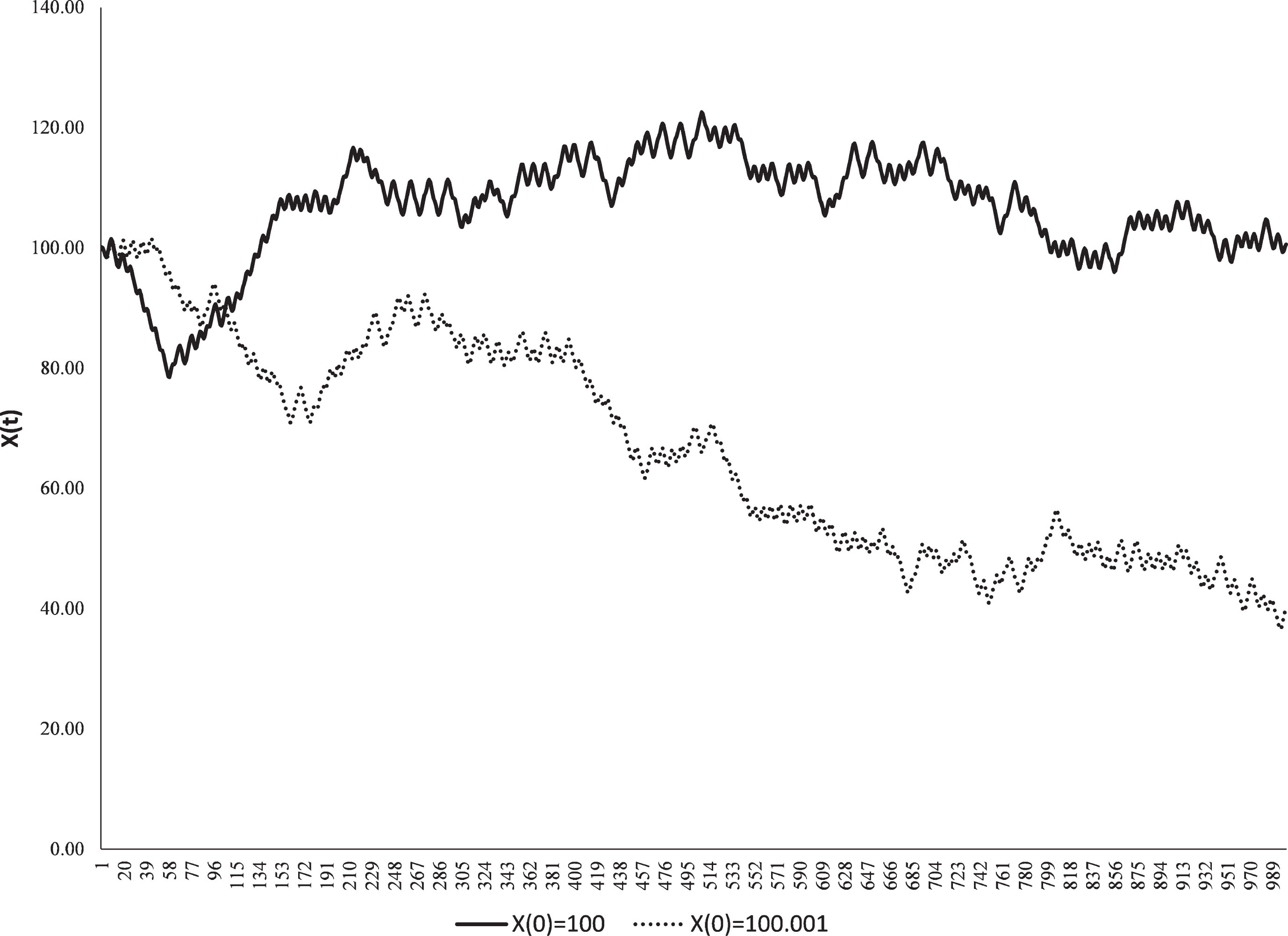
Evolution of X(t) considering small variations in the initial conditions. Source: Author’s elaboration.

The system presents an interesting symbolic dynamic that exploits the periodicity in 2π of the grid over the three axes that divide the space into an infinite number of cubes. Each cube can be subdivided into eight chambers characterized by the signs of $\dot{x}$ , $\dot{y}$ , and $\dot{z}$ . The trajectory of the three variables can be represented by an infinite sequence of symbols of an alphabet of 8 letters for which there are sequences that do not repeat. The symbol A represents the case where the differences in $\dot{x}$ , $\dot{y}$ , and $\dot{z}$ are all positive; for symbol B, the first is negative, the remaining are positive, and so on, as seen in Fig. 2. This figure also shows the transitions allowed by the symbolic model according to Sprott and Chlouverakis (2007). The symbols can be considered the vertices of the cube and the edges represent the allowed transitions, with a path entering along one edge and leaving at another.

Fig.2

Allowable transitions for symbolic sequence in the Thomas model. Source: Author’s elaboration based on the analysis conducted by Sprott and Chlouverakis (2007).

Thomas et al. (2004) introduce a generalization of the three-variable model considering n variables. This could be useful as a more general representation of the financial market. In this way, we can define: ${\dot{X}}_{i} = sin (X_{φ})$ (3) where i = 1, 2, …, n and φ = (i mod n) +1.

3 The labyrinth in the financial market

We attempt to show that labyrinth chaos, as a dynamic system, can be adapted to explain the evolution of prices in financial markets as well as in the motives and reasons that originate certain observed facts.

Before explaining the three-price model that we introduce in this study and to understand how this model can be applied to the financial markets, let us review an example of two assets presenting the economic assumptions considered in the model.

First, let us assume that for each price, there is an infinite series of equilibrium points and uncertainty zones among the equilibrium points. These prices are interrelated; what occurs at the price of one asset will impact the price of another asset. In this way, we consider that there is a lattice of equilibriums; i.e., if we consider two assets, we have to imagine the existence of a grid for which each point of intersection represents a point of equilibrium for the price pair. This grid of equilibriums is what is referred to as where the assets will walk.

Second, it must be assumed that the behavior of agents who observe the evolution of a price generates the movement of the remaining prices. Two possible explanations considered in the model are i) the agent sells or purchases an asset because a decrease or increase has been observed in the remaining assets, and ii) the agents observe the evolution of a particular price and consider that the same will occur with the remaining prices, thereby taking a position that the remaining prices generate the movement.

Let us consider an example. Suppose that there are two assets (X, Y) for which the price increases for one asset are modeled according to the sine function of the price of the other asset. First, assume, as in Fig. 3, that prices are in equilibrium at Px(0) and Py(0). Suddenly, by an external factor, such as news or the entry of a new agent, pushes the price of X to Px(1). This movement from the initial equilibrium will impact Y. Due to the type of equilibrium in which this increase is produced, it generates a decrease in the price of Y, which may have different explanations; for instance, the new price of X is more attractive, and agents start selling Y assets to purchase more of X. In this way, Y also leaves its initial equilibrium and decreases to a lower price Py(1). The decrease in the price of Y generates a decrease in the price of X, which could occur if the market is thought to be moving toward lower equilibrium prices. However, the price of X decreases to a level far below the new equilibrium to Px(2), which has a positive impact on Py, moving it to a level higher than the initial equilibrium Py(2), and the dynamics continue in this way.

Fig.3

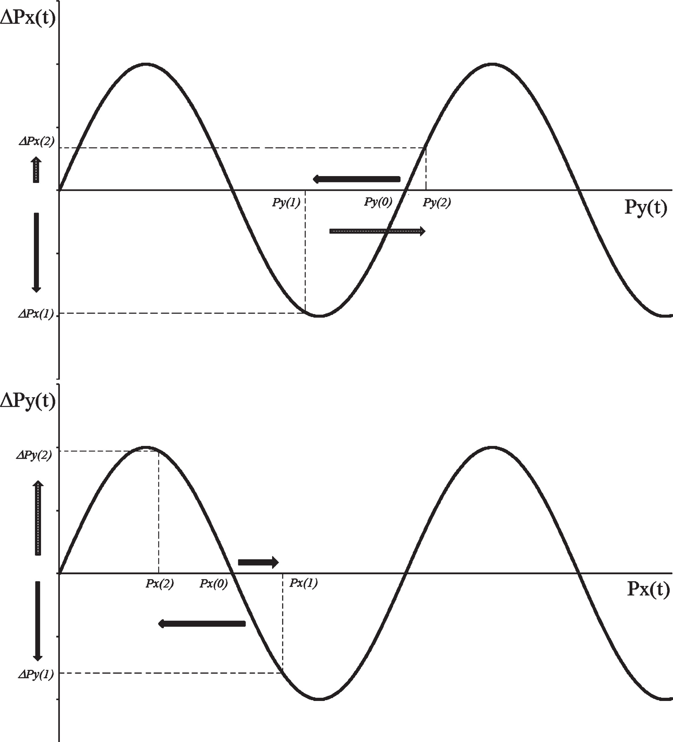
Graphical representation of the dynamics of the prices of two assets. Source: Author’s elaboration.

Note that the interaction between market prices generates a complex dynamic, causing the movement of one price to impact the movement of another price.

Considering the above example, a three-price model can be introduced by making some modifications to the original labyrinth chaos to adapt it to the dynamics of asset prices. First, we will assume that each price is affected by a linear combination of the sine function of the remaining prices. That is, the movement of the remaining market prices influences the price dynamics studied as indicated in (4). ${\begin{matrix} P_{x, t} = P_{x, t - 1} + α_{x} sin (P_{y, t - 1}) + (1 - α_{x}) sin (P_{z, t - 1}) \\ P_{y, t} = P_{y, t - 1} + α_{y} sin (P_{x, t - 1}) + (1 - α_{y}) sin (P_{z, t - 1}) \\ P_{z, t} = P_{z, t - 1} + α_{z} sin (P_{x, t - 1}) + (1 - α_{z}) sin (P_{y, t - 1}) \end{matrix}$ (4) where P_x, t, P_y, t and P_z, t represent the respective prices of x, y and z at moment t. However, α_x, α_y, and α_z are weights belonging to the closed interval [0, 1].

This system of equations can be generalized to an n-assets financial market by incorporating two additional parameters σ_i and A_i, which represent the amplitude and frequency of the sine function. The symbol of amplitude (σ_i) was selected due to its similarity with the statistical standard deviation. Each general equation of the system should be defined as follows: $P_{i, t} = P_{i, t - 1} + σ_{i} \sum_{l j = 1 j \neq 1}^{n} α_{j} sin (A_{j} P_{j, t - 1}) + γ_{i}$ (5)

For all i, j = 1, 2, … n with j ≠ i, each α_j belongs to the closed interval [0, 1], and the sum of (n - 1) α_j is equal to 1. Additionally, we can consider a constant parameter γ_i for each asset i.

To simplify the analysis, we will focus on the three-asset model and assume that α_i = 1/2, σ_i = 1 and A_i = 1. The equation system to be studied will be the following: ${\begin{matrix} P_{x, t} = P_{x, t - 1} + (1 / 2) [sin (P_{y, t - 1}) + sin (P_{z, t - 1})] + γ_{x} \\ P_{y, t} = P_{y, t - 1} + (1 / 2) [sin (P_{x, t - 1}) + sin (P_{z, t - 1})] + γ_{y} \\ P_{z, t} = P_{z, t - 1} + (1 / 2) [sin (P_{x, t - 1}) + sin (P_{y, t - 1})] + γ_{z} \end{matrix}$ (6)

First, we will assume that γ_x, γ_y, and γ_z are equal to zero.

4 Contrasting the model with empirical evidence

Table 1 presents statistical tests performed on a time series of financial prices and returns and on a simulated series using different stochastic and deterministic models.

Table 1
Tests on prices, returns and simulated series

Time ADF KPSS Variance ARCH Kolmogorov- Jarque-Bera Obs.

series test test ratio test Smirnov test test

Logistic –0.20 24.73* 0.52 0.21 0.31* 282.00* 3000

Anosov P1 –0.15 31.73* 0.94 3.81* 0.31* 169.57* 3000

Anosov P2 –0.16 31.85* –0.90 1.56 0.31* 193.65* 3000

Random Walk –0.41 44.76* 0.65 0.15 0.49* 0.01 3000

ARCH –1.25 37.83* 0.06 37.59* 0.46* 34.52* 3000

Labyrinth P1 –0.31 56.08* 34.65* 1383.13* 0.50* 44.62* 3000

Labyrinth P2 –0.44 55.84* 34.32* 1425.79* 0.50* 41.33* 3000

Labyrinth P3 –0.34 55.79* 34.62* 1361.62* 0.50* 56.49* 3000

EUR/USD –0.40 16.98* 5.82* 28.19* 0.49* 91.22* 953

USD/GBP –1.61 20.39* 7.72* 119.06* 0.48* 1835.43* 2381

US Real Estate 2.19 7.96* 3.54* 172.92* 0.46* 5621.97* 1106

Gold Fixing Price 1.18 32.57* 5.54* 46.01* 0.47* 7214.72* 2559

10 YR Bond –0.33 52.84* 2.84* 185.27* 0.47* 5184.36* 2884

20 YR Bond 0.29 12.41* 2.91* 86.53* 0.47* 452.02* 1227

NASDAQ 2.08 20.80* –0.67 106.72* 0.46* 5594.68* 2410

GSPC 2.80 62.74* –2.00 277.81* 0.47* 3621.99* 3510

NIKKEI –0.84 15.10* –0.20 27.75* 0.46* 909.12* 1377

INTC –0.07 7.62* 0.31 42.14* 0.44* 446.45* 1934

WMT 1.04 34.34* –4.35* 36.37* 0.45* 3650.81* 2328

AAPL 4.00 35.28* –1.04 19.91* 0.43* 1548.29* 2328

AXP 0.97 30.46* –1.47 172.30* 0.45* 1517.17* 2340

HD 4.26 18.6* –1.50 33.21* 0.44* 2331.57* 2466

JNJ 4.51 44.85* –0.89 183.69* 0.46* 701.50* 2466

MCD 4.71 44.64* –1.62 202.28* 0.45* 2254.73* 2466

MSFT 2.01 8.38* –0.84 20.04* 0.45* 555.81* 1621

PFE 0.98 15.30* –3.16* 62.38* 0.45* 541.14* 2340

PG 2.54 52.43* –2.52 8.75* 0.46* 18990.75* 2466

TRV 2.90 24.64* 0.26 105.21* 0.45* 1526.92* 1604

UNH 5.24 20.36* –0.88 45.80* 0.44* 3533.06* 1694

UTX 2.24 51.99* –2.09 19.07* 0.45* 2610.68* 2466

XOM 1.18 53.80* –2.36 74.29* 0.46* 501.13* 2466

BA 3.75 41.17* –2.19 37.30* 0.45* 993.68* 2883

CAT 1.01 55.22* –0.44 23.90* 0.45* 1079.68* 2883

GE 0.42 27.30* –1.84* 241.61* 0.46* 8142.78* 2883

IBM 1.15 51.45* –1.87* 45.68* 0.46* 1255.45* 2883

KO 1.85 47.34* –1.62 0.02 0.46* 2760901.14* 2883

Time	ADF	KPSS	Variance	ARCH	Kolmogorov-	Jarque-Bera	Obs.
Logistic	–0.20	24.73***	0.52	0.21	0.31***	282.00***	3000
Anosov P1	–0.15	31.73***	0.94	3.81*	0.31***	169.57***	3000
Anosov P2	–0.16	31.85***	–0.90	1.56	0.31***	193.65***	3000
Random Walk	–0.41	44.76***	0.65	0.15	0.49***	0.01	3000
ARCH	–1.25	37.83***	0.06	37.59***	0.46***	34.52***	3000
Labyrinth P1	–0.31	56.08***	34.65***	1383.13***	0.50***	44.62***	3000
Labyrinth P2	–0.44	55.84***	34.32***	1425.79***	0.50***	41.33***	3000
Labyrinth P3	–0.34	55.79***	34.62***	1361.62***	0.50***	56.49***	3000
EUR/USD	–0.40	16.98***	5.82***	28.19***	0.49***	91.22***	953
USD/GBP	–1.61	20.39***	7.72***	119.06***	0.48***	1835.43***	2381
US Real Estate	2.19	7.96***	3.54***	172.92***	0.46***	5621.97***	1106
Gold Fixing Price	1.18	32.57***	5.54***	46.01***	0.47***	7214.72***	2559
10 YR Bond	–0.33	52.84***	2.84***	185.27***	0.47***	5184.36***	2884
20 YR Bond	0.29	12.41***	2.91***	86.53***	0.47***	452.02***	1227
NASDAQ	2.08	20.80***	–0.67	106.72***	0.46***	5594.68***	2410
GSPC	2.80	62.74***	–2.00**	277.81***	0.47***	3621.99***	3510
NIKKEI	–0.84	15.10***	–0.20	27.75***	0.46***	909.12***	1377
INTC	–0.07	7.62***	0.31	42.14***	0.44***	446.45***	1934
WMT	1.04	34.34***	–4.35***	36.37***	0.45***	3650.81***	2328
AAPL	4.00	35.28***	–1.04	19.91***	0.43***	1548.29***	2328
AXP	0.97	30.46***	–1.47	172.30***	0.45***	1517.17***	2340
HD	4.26	18.6***	–1.50	33.21***	0.44***	2331.57***	2466
JNJ	4.51	44.85***	–0.89	183.69***	0.46***	701.50***	2466
MCD	4.71	44.64***	–1.62	202.28***	0.45***	2254.73***	2466
MSFT	2.01	8.38***	–0.84	20.04***	0.45***	555.81***	1621
PFE	0.98	15.30***	–3.16***	62.38***	0.45***	541.14***	2340
PG	2.54	52.43***	–2.52**	8.75***	0.46***	18990.75***	2466
TRV	2.90	24.64***	0.26	105.21***	0.45***	1526.92***	1604
UNH	5.24	20.36***	–0.88	45.80***	0.44***	3533.06***	1694
UTX	2.24	51.99***	–2.09**	19.07***	0.45***	2610.68***	2466
XOM	1.18	53.80***	–2.36**	74.29***	0.46***	501.13***	2466
BA	3.75	41.17***	–2.19**	37.30***	0.45***	993.68***	2883
CAT	1.01	55.22***	–0.44	23.90***	0.45***	1079.68***	2883
GE	0.42	27.30***	–1.84*	241.61***	0.46***	8142.78***	2883
IBM	1.15	51.45***	–1.87*	45.68***	0.46***	1255.45***	2883
KO	1.85	47.34***	–1.62	0.02	0.46***	2760901.14***	2883

Source: Author’s elaboration based on weekly data and data simulated by MATLAB. The ARCH model considers the same parameters presented in Hsieh (1991). In the case of the adjusted labyrinth chaos, the initial conditions are p1(0) = 204, p2(0) = 210, and p3(0) = 216. For the remainder of the models, the initial price was 200. ***indicates significance at p-value <0.01; **indicates significance at p-value <0.05; *indicates significance at p-value <0.10.

The purpose of this exercise is to analyze the characteristics of the financial markets and compare them with those produced with most known models, such as the classic random walk or the random walk adjusted by ARCH processes, as well as those produced by deterministic chaotic models. One of these chaotic models used in this analysis is the adjusted labyrinth chaos.

First, we apply the Dickey-Fuller unit root tests, the KPSS test and the variance ratio test on the series in levels. Then, we apply the ARCH test, the Kolmogorov-Smirnov normality test and the Jarque-Bera test on the returns.

Note that all series, such as prices, indices, currencies or even price series that are simulated by stochastic or deterministic models would present a unit root according to the ADF test or would be rejected as stationary processes according to the KPSS test. In this sense, all the selected models would reproduce the behavior of the real-time series.

The variance ratio shows different results and in part, this is consistent with the behavior of the real-time series. First, it is clear that the variance ratio rejects the null hypothesis in the cases of price relations, commodities such as gold, real estate, treasury bonds, stock indices and financial stock assets. Second, chaotic processes such as Anosov and logistic processes do not reject this hypothesis. This also occurs with the random walk process and the random walk adjusted by GARCH. However, in the case of the labyrinth, the variance ratio null hypothesis is rejected, as in the case of many of the real-time series.

Either the heteroskedasticity test on the standard deviation of the residuals of the returns or the ARCH test was applied. With the exception of Coca Cola (KO), all the real-time series reject the homoscedasticity of returns. As previously mentioned, this occurs because of volatility clustering, which would indicate that the ARCH models would be a good fit for the variance of the returns. In fact, the test is not rejected in the case of the common random walk, but the random walk adjusted by ARCH shows the same characteristics of the series. However, the logistical model and the Anosov model would not reproduce this, except in the case of one of the series in the latter model. In the case of the adjusted labyrinth chaos model, this is reproduced in the three series.

Finally, both the Kolmogorov-Smirnov test and the Jarque-Bera normality test reject normality in all financial series, as do all the proposed models. The only exception is that the Jarque-Bera test does not reject normality in the random walk.

In this way, the ARCH and adjusted labyrinth chaos models reproduce the phenomena observed in the financial time series. This does not occur with the common random walk, nor does it occur with the simple logistic model or the Anosov model.

As a second experiment, 10,000 Monte Carlo simulations were conducted for the GARCH model and the adjusted labyrinth chaos model, obtaining almost one and a half million observations. Table 2 shows the results of the application of the above tests to the series and their growth rates. Note that both the ADF and the KPSS tests indicate that the processes would be non-stationary. In fact, the unit root hypothesis is rejected 15.22% of the time in the case of the ADF and 5.12% of the time in the case of the GARCH model. However, the hypothesis of stationarity of the KPSS test is rejected 99.62% of the time in the case of the labyrinth and 100% of the time in the case of the GARCH model. The result the test variance ratio shows different results; the labyrinth rejects the test 100% of the time, and the model GARCH rejects the test 5.04% of the time. Notably, as shown in Table 1, the financial series do not appear to have a clear definition on this issue.

Table 2

Percent rejection of the tests applied to the labyrinth and GARCH models

Test	Labyrinth	GARCH
ADF	15.22%	5.12%
KPSS	99.62%	100.00%
Variance Ratio	100.00%	5.04%
ARCH	99.95%	99.99%
Kolmogorov-Smirnov	100.00%	100.00%
Jarque-Bera	94.94%	74.32%

Source: Author’s elaboration. The GARCH model is the same as used by Hsieh (1991).

The ARCH test rejects homoscedasticity of the variance in 99.95% of the cases for the adjusted labyrinth chaos model and 99.99% of the cases for the GARCH model. As mentioned before, ARCH-type models were designed to reproduce this type of behavior, but there is no explanation regarding the causes. The novel issue here is that the proposed chaotic model generates the same type of behavior, but the explanation originates in the dynamic interaction between the prices.

Figure 4 shows how volatility clustering is manifested in the adjusted labyrinth chaos model with a constant (γ = 0.00001) as in the real financial time series. Note that the S&P 500 daily returns present certain periods in which volatility is greater and other periods in which volatility is lower; this phenomenon is also observed in the series originated by the chaotic system. Note that even the jump issue is produced in the chaotic system. Note also that as Engle (2004) asserted, volatility is higher when prices are falling. Volatility tends to be higher in bear markets. In fact, Nelson (1991) remarks that the major episodes of high volatility are associated with market drops.

Fig.4

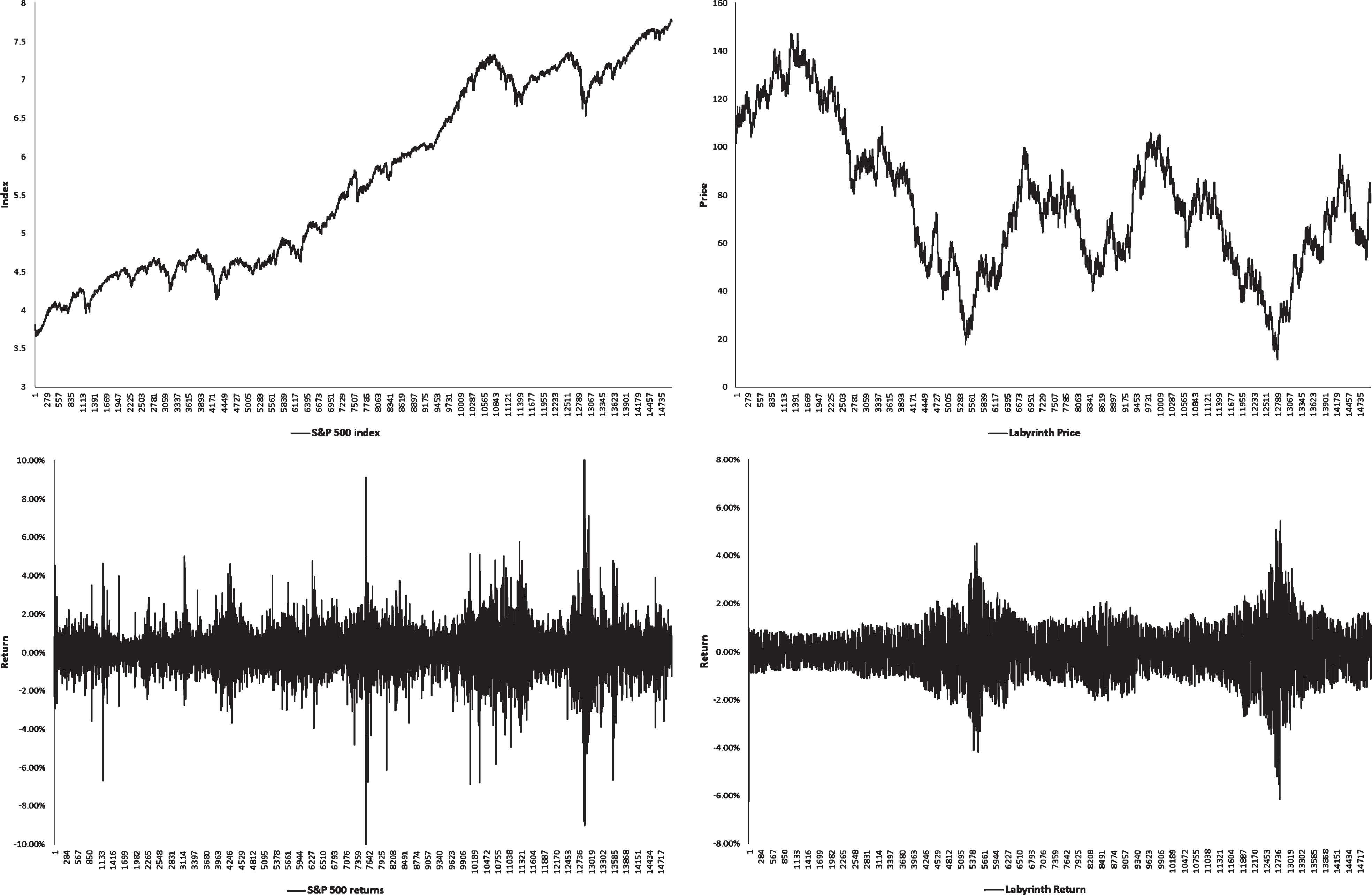
Volatility clustering in the S&P 500 index and the adjusted labyrinth chaos. Source: Author’s elaboration. The series Y is plotted from the labyrinth model considering initial conditions X₀= 219, Y₀= 200 and Z₀= 206 and a constant equal to 0.00001 in each equation.

Finally, both the Kolmogorov-Smirnov and Jarque-Bera tests show a high percentage of rejection of normal returns in both series. That is, 100% rejection in the case of the Kolmogorov-Smirnov test and 94.94% and 74.32% in the case of Jarque-Bera test. Figure 5 shows the histogram of the labyrinth and S&P returns compared to a Gaussian density. It can be observed that neither series behaves as a normal density. In fact, both series are leptokurtic and have negative asymmetry. In the case of the S&P 500, the kurtosis is 23.85, and the kurtosis of the labyrinth is 5.59; in both cases, there is a greater than normal distribution corresponding to 3. The Jarque-Bera test rejects the normality of the series with a statistic of 272,715.58 and 4,202.66 for the S&P 500 and labyrinth cases, respectively, which is well above the critical value of 5.99 to 5% of a Chi-2 with 2 degrees of freedom.

Fig.5

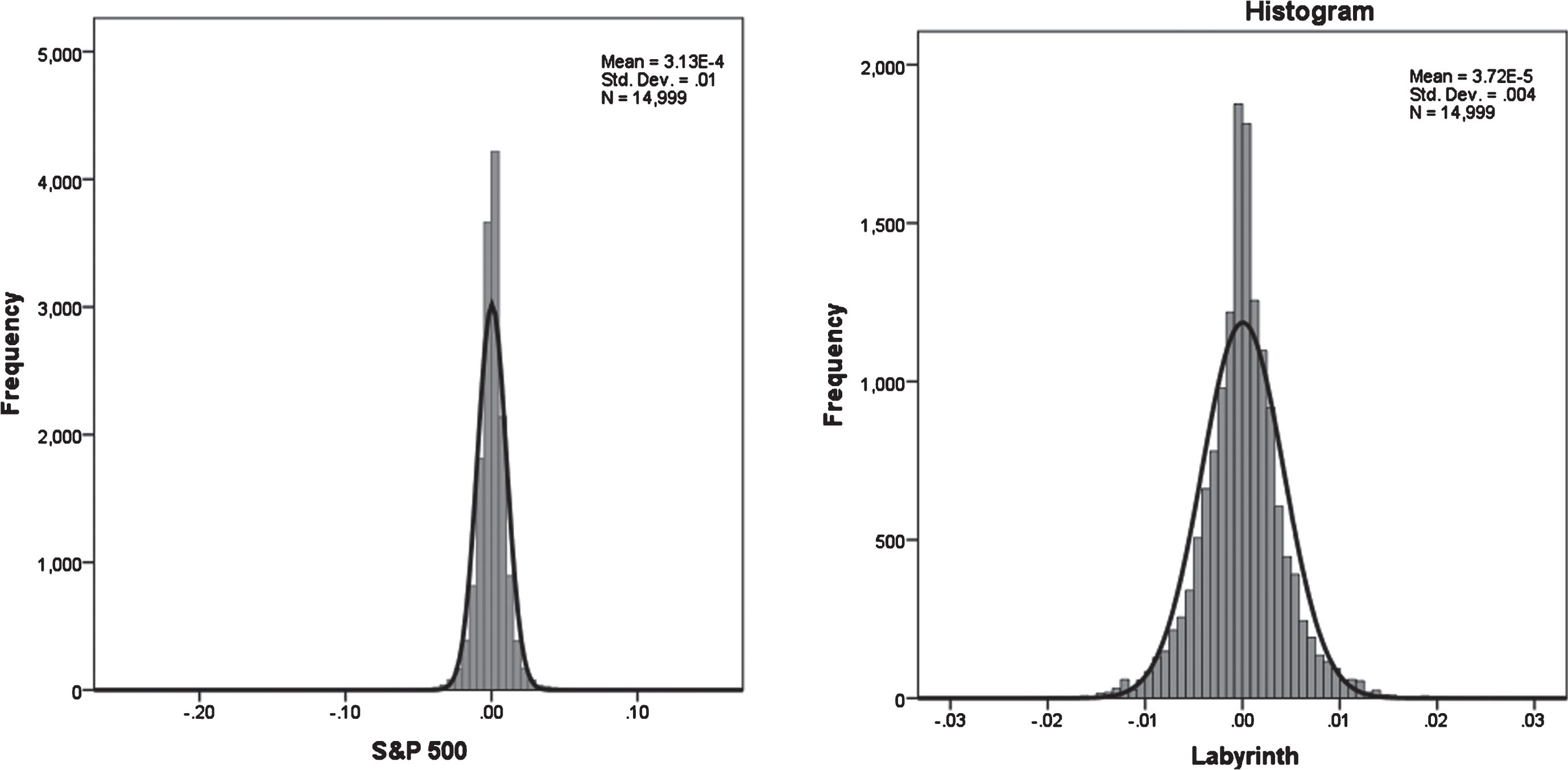
Histogram of the returns of S&P 500 and the adjusted labyrinth chaos. Source: Author’s elaboration.

Note that the phenomenon of heavy tails in the model is related to the volatility clustering that originates in the very dynamics of the chaotic system. It is interesting to note in Table 3 that a series originated in a completely deterministic model such as the labyrinth chaos, perfectly fits a GARCH stochastic model, which is similar to the S&P 500 financial index.

Table 3

Estimation of the model AR(1)-GARCH(1,1) for the S&P 500 and labyrinth

Parameter	S&P 500	Labyrinth
C	0.001***	0.000
AR(1)	0.083***	0.814***
Equation of the variance
C	0.000***	0.000***
RESID(–1)²	0.086***	0.716***
GARCH(–1)	0.908***	0.365***

Source: Author’s elaboration. The software Eviews 9.0 was applied. *** indicates significance at p-value <0.01.

As a next step, a symbolic analysis was carried out by performing a numerical analysis beginning with 5,000 different initial conditions and in each case, 30,000 observations of the model were run. Based on the aforementioned symbolic study by Sprott and Chlouverakis (2007), a symbolization of 8 letters A, B, C, D, E, F, G, and H was used according to whether each of the three series has a negative or positive value and their combinations, which generates information about the dynamics of the system. Following the symbolic analysis presented by these authors, the symbol A occurs when the increases for all three variables are positive, the symbol B occurs when the first variable has a negative increase and the remaining variables have positive increases and so on, as shown in Fig. 6. This figure also shows the transitions allowed by the symbolic model applied to the financial market. These symbols can be considered the vertices of a hexagonal bipyramid, and the edges represent the allowed transitions, with a path entering along one edge and leaving along another. Notably, the dynamics of the proposed model are different from those presented by the cube arising from the original Thomas model. Note that we can find similar symbolic analyzes in finance, for instance, Maymin (2011) considers transition diagrams for different sell-buy rules generating complex price paths.

Fig.6

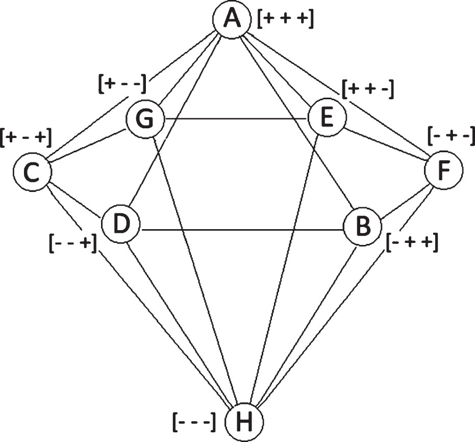
Allowed transitions in the financial model. Source: Author’s elaboration.

In this way, weekly data from the first week of January 1999 until the first of April 2017 (952 observations of returns) were obtained from an exchange market composed of the EUR/USD, USD/GBP and JPY/USD currencies. A stock market composed of the DAX, NIKKEI and S&P 500 indices was also considered from the last week of November 1990 until the second week of April 2017 (1376 observations of returns). Finally, we considered the labyrinth chaos model that has been analyzed.

We also compared the results with a GARCH model that randomly generated three sets of financial returns according to the following expression presented by Hsieh (1991): $r_{t} = σ_{t} μ_{t}$ (7) $σ_{t}^{2} = 1 + 0.1 r_{t - 1}^{2} + 0.8 σ_{t - 1}^{2}$

However, to analyze the possible effect of correlation between the assets, first, a VAR model was estimated with the returns of the three stock indices mentioned above. This model was used to generate random numbers and the three series of returns to be analyzed symbolically. The final model used for this analysis is the following: ${\begin{matrix} r_{1, t} = 0.01 - 0.12 r_{1, t - 1} - 0.05 r_{2, t - 1} + 0.21 r_{3, t - 1} + ɛ_{1, t} \\ r_{2, t} = - 0.01 + 0.03 r_{1, t - 1} - 0.11 r_{2, t - 1} + 0.20 r_{3, t - 1} + ɛ_{2, t} \\ r_{3, t} = 0.01 + 0.01 r_{1, t - 1} - 0.03 r_{2, t - 1} - 0.07 r_{3, t - 1} + ɛ_{3, t} \end{matrix}$ (8) where ɛ₁, ɛ₂ and ɛ₃ are normal random processes with a mean of 0 and standard deviation equal to 0.03, 0.03 and 0.02, respectively, that originated in the econometric estimation of the model.

Using sequences of 3 symbols results in 512 (8³) combinations. Notably, in Table 4, only the labyrinth is capable of reproducing some of the first five behaviors. The FOREX market is able to detect the pattern [EEE], which implies that for three weeks in a row, the returns of the first two currencies are positive, and the third currency is negative. In the case of the Indices, the patterns [AAA] and [HHH] are detected in both the three indices and in the labyrinth; this does not occur for any of the GARCH models or for the VAR model. These two dynamic patterns imply that for three consecutive weeks, there were either positive returns for all three indices or negative returns for all three indices, respectively.

Table 4

Most common dynamic patterns in the FOREX, indices and simulated models

FOREX		Labyrinth		GARCH		VAR
[EEE]	3.16	[HHH]	10.95	[CCF]	0.74	[CCC]	1.79
[DDD]	2.63	[AAA]	7.79	[DDH]	0.74	[CCA]	1.37
[EDD]	2.00	[EEE]	2.84	[BBG]	0.63	[CAC]	1.26
[DDH]	1.47	[FFF]	2.74	[CFA]	0.63	[ACA]	1.16
[AEE]	1.37	[HHF]	2.32	[FDD]	0.63	[DCA]	1.16
Indices		Labyrinth		GARCH		VAR
[AAA]	2.55	[HHH]	10.42	[CCF]	0.58	[CCC]	1.67
[AHA]	2.33	[AAA]	8.16	[CFA]	0.58	[CAC]	1.46
[HAA]	2.26	[EEE]	2.62	[EBB]	0.58	[CCA]	1.46
[AAH]	1.97	[FFF]	2.55	[FEB]	0.58	[CAD]	1.31
[HHH]	1.82	[HHF]	2.04	[ADD]	0.51	[ACA]	1.16

Source: Author’s elaboration.

However, we detect dynamic patterns that have not yet been covered. That is, in a random process, it would be expected that all combinations would be run with the same frequency. In the case of FOREX, where there are 952 weeks of returns, there are 179 non-traded patterns of the 512 possible; there are 381 possible patterns for the labyrinth and 184 for the VAR model. It is emphasized that in the case of GARCH processes, 84 patterns are not traveled in 952 observations.

In the case of stock indices with 1376 observations, 145 non-traded patterns are observed; with this same number of observations the labyrinth has 377 patterns, the VAR model falls to 139, and the GARCH models fall to only 34 patterns. On one hand, this means that the GARCH models, independently of each other, correspond to a random walk in space, traversing in a homogeneous manner through all the sectors of space. On the other hand, this could suggest the existence of a correlation between the indices that is collected by both a VAR model and the labyrinth. For the latter, the matching patterns between the models will be analyzed.

The GARCH model has only 24 patterns matching FOREX and only 10 with indices, while the VAR has 63 patterns with FOREX and 46 with indices. However, the labyrinth is able to detect 110 dynamic patterns for which the indices have not passed and 142 for which the three active FOREX market has not passed.

As a summary, Table 5 shows the 42 combinations that do not appear in the indices, the FOREX market, or the adjusted labyrinth chaos. For example, [BCB] means that neither the labyrinth nor any of the markets displayed the following: the first week, the first asset had a negative return, and the other two had positive returns; in the second week, the first and third assets had returns that were positive, and the second a negative return; and in the third week, the assets repeat the same behavior as the first week. That is, it has not been observed that the return of the first asset is negative and that of the other two is positive. These patterns should also be compared in light of the allowed transitions of Fig. 6. Note that both [BC] and [CB] are non-allowed transitions in the labyrinth model.

Table 5

Combinations that do not appear in the indices, FOREX or the labyrinth

[BCB]	[CDB]	[FBD]	[GDF]
[BDF]	[CDE]	[FBG]	[GDG]
[BEF]	[CEG]	[FEC]	[GFC]
[BFG]	[CFG]	[FEH]	[GFD]
[BGA]	[CGF]	[FFC]	[GFG]
[BGB]	[DBC]	[FGB]	[GGF]
[BGD]	[DFB]	[FHF]	[GHF]
[BGF]	[DHB]	[GBF]	[HBB]
[BHB]	[EBF]	[GCB]	[HBC]
[CBF]	[EBG]	[GCF]	[HBG]
[CBG]	[FAC]

Source: Author’s elaboration.

Although the main objective of the presented model is to attempt to provide a possible explanation for the characteristics of financial assets, in this section, an attempt is made to appreciate the ability to predict a model of this type in comparison with some that are already known. First, it was determined whether any transformation must be made to the variables for the labyrinth chaos model to produce better results. To analyze this issue, we proceeded to use stock series, considering a moving window of 50 observations and dynamically projecting a period (10 periods of time and 100 periods) to later compare the projections with the data observed in reality through indicators such as MAPE, MPE and Theil U. Once these projections were made, the average value of these indicators was calculated, and it was observed that this occurs when the base of the series used is changed. In a deterministic model such as the chaotic one in which the frequency (A) and the amplitude (σ) of the sine function are fixed, the transformation or change of the base of the value of the series is not trivial. However, it should be noted that this consideration has no effect on the GARCH models that are based on returns and not on prices, nor does this consideration impact the VAR models applied here that also use returns.

A series of projection exercises shows that the prediction capability improves around the normalization value of 200. Figure 7 shows the mean of the MAPE indicator in the case of the projection of the relationship between the British pound sterling and the dollar (GBPUSD) based on base price changes for projections of 1 month, 10 months and 100 months.

Fig.7

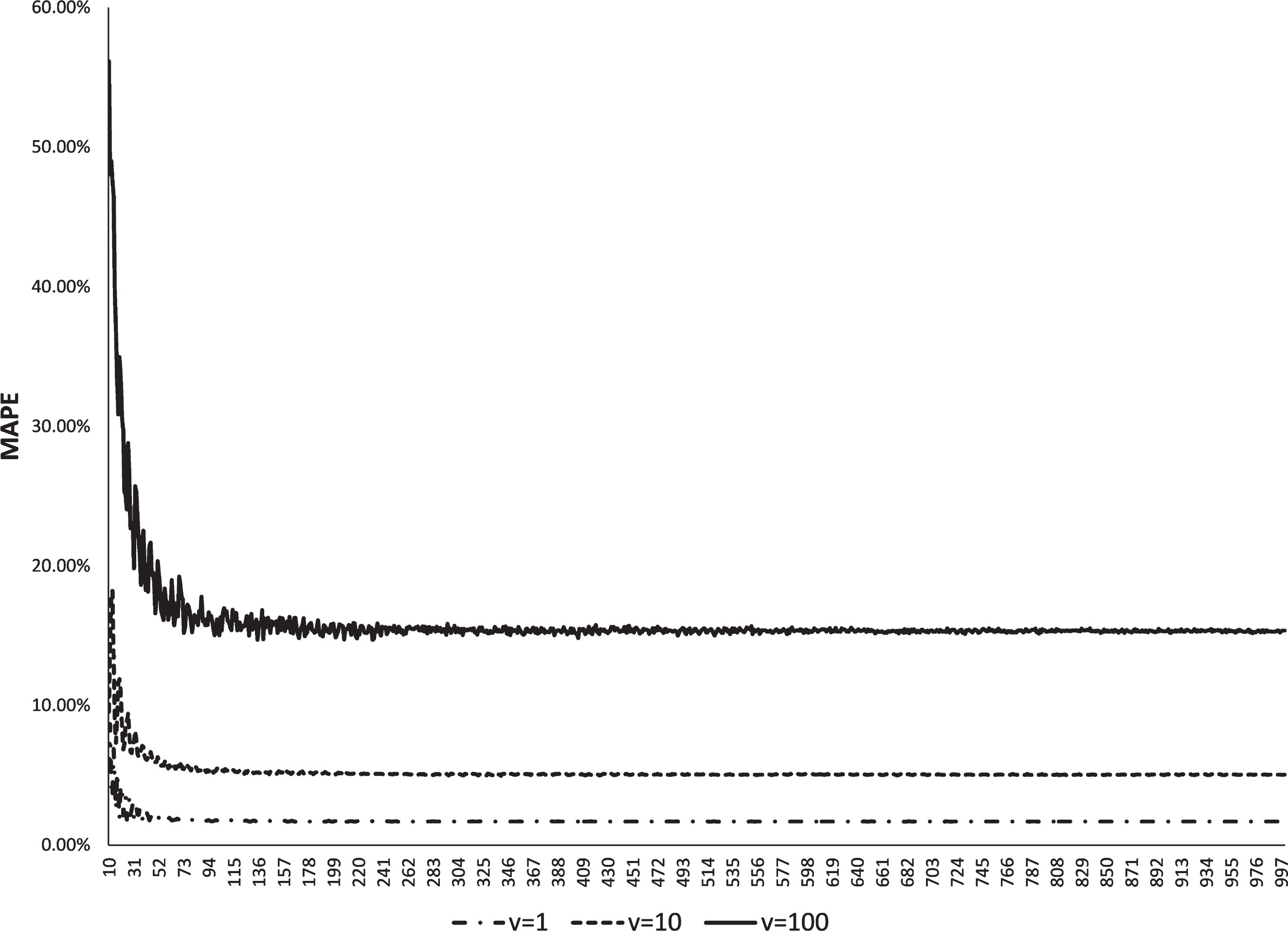
Mean of the MAPE error as a function of the normalization value of the monthly GBPUSD series. Source: Author’s elaboration.

First, a smaller error is observed as less projection, and an improvement in the projection is observed, as larger normalization values are used. It could be said that in this particular case, from 100, the prediction error is stabilized.

We proceeded to compare the predictive capacity of the labyrinth model with well-known econometric models and some form of naif projection. Three stocks (General Motors, IBM and Boeing) were randomly selected, and three global stock indices DJI, NIKKEI and FTSE were chosen. Likewise, three relationships were chosen between the FOREX market currencies, such as the relation between the euro and the dollar (EUR/USD), the relation between the pound and the dollar (GBP/USD) and the dollar and yen (USD/JPY). Finally, three other assets were considered, such as the yield on 20-year US bonds, gold (gold fixing price) and a real estate index (Wilshire US Real Estate). The data were obtained monthly and the time periods differ depending on the availability of the data. Shares began in January 1962, the indices in April 1984, the currencies in January 1999 and the remainder of the assets in October 1993; all end in March 2017.

The following models were chosen for the comparison: i) a simple projection taking the average of the past returns to project the future price (naif model); ii) an AR (1) -GARCH (1,1) model that, as mentioned, is widely used in stock market assets; iii) a VAR model (1) on returns of three series, due to the attempt to apply a model that shows interaction between prices; and finally, iv) a labyrinth model, presented in the system of Equations (6), where a second version of the labyrinth model was applied, which will include the estimation of the standard deviation of the series as an amplitude of the sine function, as shown in the system of Equations (7). ${\begin{matrix} P_{x, t} = P_{x, t - 1} + (1 / 2) σ_{x} [sin (P_{y, t - 1}) + sin (P_{z, t - 1})] \\ P_{y, t} = P_{y, t - 1} + (1 / 2) σ_{y} [sin (P_{x, t - 1}) + sin (P_{z, t - 1})] \\ P_{z, t} = P_{x, t - 1} + (1 / 2) σ_{z} [sin (P_{x, t - 1}) + sin (P_{y, t - 1})] \end{matrix}$ (7)

Tables 6 –9 show the average errors and their standard deviations when moving projections of the series were taken, beginning with an initial window of 50 months that grew as the dynamics of the observations progressed.

Table 6

Mean and standard deviation of the prediction error in actions

Projecting 1	GE	IBM	BA
Naïf
MAPE	5.23% (4.72%)	5.25% (4.64%)	7.16% (6.31%)
MPE	–0.34% (7.04%)	–0.41% (7.00%)	–0.93% (9.50%)
U	2.60% (2.27%)	2.61% (2.25%)	3.53% (2.97%)
AR-GARCH
MAPE	5.26% (4.74%)	5.32% (4.63%)	7.17% (6.29%)
MPE	–0.50% (7.07%)	–0.56% (7.03%)	–1.07% (9.48%)
U	2.61% (2.27%)	2.64% (2.25%)	3.53% (2.96%)
VAR
MAPE	4.79% (4.21%)	5.01% (4.56%)	7.19% (6.30%)
MPE	0.44% (6.36%)	0.24% (6.77%)	0.09% (9.56%)
U	2.40% (2.08%)	2.51% (2.25%)	3.58% (3.03%)
Labyrinth
MAPE	5.18% (4.69%)	5.21% (4.60%)	7.12% (6.12%)
MPE	0.54% (6.97%)	0.44% (6.94%)	0.27% (9.39%)
U	2.60% (2.30%)	2.61% (2.27%)	3.55% (2.94%)
Labyrinth 2
MAPE	5.18% (4.69%)	5.21% (4.58%)	7.11% (6.11%)
MPE	0.54% (6.97%)	0.45% (6.93%)	0.27% (9.38%)
U	2.60% (2.30%)	2.61% (2.26%)	3.55% (2.94%)
Projecting 10	GE	IBM	BA
Naïf
MAPE	12.12% (12.36%)	12.58% (9.00%)	18.63% (14.66%)
MPE	–1.96% (16.69%)	–2.37% (14.55%)	–5.80% (22.24%)
U	6.56% (4.74%)	7.01% (4.24%)	9.93% (6.39%)
AR-GARCH
MAPE	12.20% (12.61%)	12.71% (9.15%)	18.66% (14.55%)
MPE	–2.78% (16.80%)	–3.21% (14.60%)	–6.51% (21.98%)
U	6.53% (4.75%)	7.00% (4.21%)	9.90% (6.36%)
VAR
MAPE	12.23% (10.33%)	12.16% (7.91%)	17.69% (11.77%)
MPE	2.87% (15.14%)	2.14% (13.56%)	0.77% (20.42%)
U	7.09% (4.51%)	7.19% (4.33%)	10.26% (6.18%)
Labyrinth
MAPE	12.47% (10.59%)	12.29% (7.84%)	17.63% (11.68%)
MPE	2.86% (15.55%)	2.37% (13.58%)	1.07% (20.30%)
U	7.20% (4.55%)	7.26% (4.29%)	10.22% (6.06%)
Labyrinth 2
MAPE	12.45% (10.52%)	12.27% (7.58%)	17.63% (11.67%)
MPE	2.90% (15.46%)	2.39% (13.57%)	1.06% (20.29%)
U	7.19% (4.53%)	7.25% (4.30%)	10.23% (6.05%)
Projecting 100	GE	IBM	BA
Naïf
MAPE	59.55% (55.28%)	51.49% (34.43%)	129.30% (288.54%)
MPE	–25.89% (75.88%)	–26.81% (53.44%)	–102.90% (298.16%)
U	30.06% (13.03%)	25.98% (13.58%)	34.91% (19.97%)
AR-GARCH
MAPE	63.48% (61.82%)	57.79% (41.27%)	114.58% (181.82%)
MPE	–34.79% (80.31%)	–37.88% (57.91%)	–89.95% (193.94%)
U	29.45% (13.69%)	26.57% (13.86%)	37.15% (18.01%)
VAR
MAPE	40.09% (14.32%)	33.64% (15.31%)	54.98% (55.18%)
MPE	22.03% (34.31%)	19.06% (27.57%)	9.54% (74.32%)
U	34.14% (18.87%)	27.79% (17.41%)	37.31% (17.49%)
Labyrinth
MAPE	40.20% (14.30%)	33.88% (15.31%)	53.83% (48.17%)
MPE	21.94% (34.43%)	19.22% (27.71%)	10.72% (68.15%)
U	34.18% (18.88%)	27.93% (17.41%)	37.25% (17.44%)
Labyrinth 2
MAPE	40.07% (14.28%)	33.72% (15.27%)	53.98% (48.52%)
MPE	22.02% (34.25%)	19.30% (27.45%)	10.67% (68.55%)
U	34.12% (18.94%)	27.87% (17.44%)	37.30% (17.42%)
Observations	664	664	664

Source: Author’s elaboration. The standard deviation of the prediction errors is presented in parentheses.

Table 7

Mean and standard deviation of prediction error in and stock indices

Projecting 1	DJI	NIKKEI	FTSE
Naïf
MAPE	3.06% (2.87%)	4.83% (4.23%)	3.17% (2.77%)
MPE	–0.47% (4.17%)	–0.81% (6.37%)	–0.51% (4.18%)
U	1.52% (1.38%)	2.38% (2.00%)	1.57% (1.35%)
AR-GARCH
MAPE	3.07% (2.88%)	4.87% (4.28%)	3.18% (2.79%)
MPE	–0.44% (4.19%)	–1.08% (6.40%)	–0.54% (4.20%)
U	1.52% (1.38%)	2.40% (2.03%)	1.57% (1.35%)
VAR
MAPE	3.20% (2.81%)	4.89% (4.20%)	3.28% (2.71%)
MPE	0.52% (4.23%)	–0.49% (6.43%)	0.29% (4.25%)
U	1.60% (1.38%)	2.42% (2.02%)	1.64% (1.34%)
Labyrinth
MAPE	3.15% (2.68%)	4.76% (4.09%)	3.19% (2.62%)
MPE	0.59% (4.10%)	–0.30% (6.27%)	0.30% (4.12%)
U	1.58% (1.32%)	2.36% (1.95%)	1.59% (1.30%)
Labyrinth 2
MAPE	3.15% (2.71%)	4.78% (4.09%)	3.19% (2.65%)
MPE	0.57% (4.12%)	–0.31% (6.29%)	0.31% (4.14%)
U	1.58% (1.33%)	2.37% (1.96%)	1.59% (1.31%)
Projecting 10	DJI	NIKKEI	FTSE
Naïf
MAPE	7.12% (6.39%)	13.16% (9.39%)	7.40% (6.14%)
MPE	–2.71% (8.87%)	–5.04% (14.83%)	–2.92% (8.82%)
U	3.91% (2.91%)	7.03% (4.08%)	4.04% (2.84%)
AR-GARCH
MAPE	7.14% (6.25%)	13.80% (10.00%)	7.38% (6.07%)
MPE	–2.48% (8.86%)	–6.77% (15.13%)	–2.99% (8.74%)
U	3.93% (2.86%)	7.24% (4.26%)	4.03% (2.81%)
VAR
MAPE	7.50% (5.25%)	12.18% (7.85%)	7.49% (4.92%)
MPE	2.98% (8.29%)	–2.27% (13.74%)	1.66% (8.42%)
U	4.42% (2.70%)	6.73% (3.61%)	4.33% (2.47%)
Labyrinth
MAPE	7.55% (5.25%)	12.09% (7.66%)	7.44% (4.84%)
MPE	3.06% (8.28%)	–2.01% (13.58%)	1.65% (8.32%)
U	4.45% (2.68%)	6.70% (3.54%)	4.30% (2.42%)
Labyrinth 2
MAPE	7.50% (5.24%)	12.09% (7.68%)	7.40% (4.90%)
MPE	3.02% (8.26%)	–2.03% (13.60%)	1.66% (8.32%)
U	4.42% (2.68%)	6.70% (3.55%)	4.28% (2.46%)
Projecting 100	DJI	NIKKEI	FTSE
Naïf
MAPE	46.60% (29.76%)	101.79% (107.11%)	45.23% (33.43%)
MPE	–40.56% (36.20%)	–95.26% (112.09%)	–41.39% (36.09%)
U	21.34% (10.58%)	30.09% (16.53%)	19.83% (10.69%)
AR-GARCH
MAPE	42.56% (24.32%)	138.03% (113.06%)	43.23% (29.38%)
MPE	–35.6% (32.39%)	–133.47% (117.44%)	–39.55% (31.95%)
U	20.11% (9.00%)	37.48% (17.91%)	19.36% (9.66%)
VAR
MAPE	26.10% (12.83%)	35.66% (16.84%)	23.22% (8.34%)
MPE	20.78% (18.13%)	–25.42% (26.56%)	12.03% (20.05%)
U	21.11% (13.42%))	16.25% (4.89%)	16.71% (8.64%)
Labyrinth
MAPE	26.52% (12.75%)	35.08% (16.00%)	23.49% (8.45%)
MPE	21.04% (18.33%)	–24.56% (25.92%)	12.25% (20.22%)
U	21.43% (13.45%)	16.15% (4.75%)	16.91% (8.69%)
Labyrinth 2
MAPE	26.16% (12.80%)	35.25% (16.21%)	23.18% (8.22%)
MPE	20.88% (18.10%)	–24.96% (25.98%)	12.01% (19.98%)
U	21.16% (13.41%)	16.15% (4.76%)	16.69% (8.57%)
Observations	397	397	397

Source: Author’s elaboration. The standard deviation of the prediction errors is presented in parentheses.

Table 8

Mean and standard deviation of the prediction error in currencies

Projecting 1	EUR/USD	USD/JPY	GBP/USD
Naïf
MAPE	1.84% (1.52%)	1.82% (1.54%)	1.71% (1.58%)
MPE	–0.15% (2.39%)	–0.01% (2.39%)	–0.22% (2.32%)
U	0.92% (0.75%)	0.91% (0.77%)	0.85% (0.78%)
AR-GARCH
MAPE	1.83% (1.42%)	1.81% (1.45%)	1.70% (1.49%)
MPE	–0.17% (2.31%)	–0.03% (2.32%)	–0.18% (2.26%)
U	0.91% (0.71%)	0.90% (0.72%)	0.85% (0.73%)
VAR
MAPE	1.83% (1.53%)	1.86% (1.44%)	1.76% (1.49%)
MPE	–0.08% (2.39%)	0.03% (2.35%)	–0.15% (2.30%)
U	0.91% (0.76%)	0.93% (0.72%)	0.88% (0.73%)
Labyrinth
MAPE	1.88% (1.52%)	1.83% (1.50%)	1.73% (1.55%)
MPE	–0.01% (2.42%)	–0.06% (2.37%)	–0.17% (2.32%)
U	0.94% (0.75%)	0.91% (0.75%)	0.86% (0.76%)
Labyrinth 2
MAPE	1.83% (1.50%)	1.82% (1.52%)	1.70% (1.58%)
MPE	–0.03% (2.38%)	–0.06% (2.38%)	–0.17% (2.32%)
U	0.92% (0.75%)	0.91% (0.76%)	0.85% (0.78%)
Projecting 10	EUR/USD	USD/JPY	GBP/USD
Naïf
MAPE	5.31% (3.51%)	5.24% (3.31%)	5.14% (4.47%)
MPE	–0.99% (6.07%)	–0.35% (5.96%)	–1.33% (6.52%)
U	2.97% (1.75%)	3.03% (1.90%)	2.85% (2.19%)
AR-GARCH
MAPE	5.42% (3.62%)	5.21% (3.28%)	5.13% (4.41%)
MPE	–1.34% (6.19%)	–0.35% (5.91%)	–1.28% (6.48%)
U	3.03% (1.81%)	3.02% (1.66%)	2.85% (2.16%)
VAR
MAPE	5.36% (3.29%)	5.28% (3.26%)	5.20% (4.38%)
MPE	–0.50% (6.08%)	–0.41% (5.95%)	–1.08% (6.56%)
U	3.01% (1.64%)	3.03% (1.90%)	2.89% (2.14%)
Labyrinth
MAPE	5.36% (3.27%)	5.22% (3.25%)	5.17% (4.34%)
MPE	–0.26% (6.06%)	–0.56% (5.86%)	–1.03% (6.50%)
U	3.02% (1.66%)	3.01% (1.81%)	2.88% (2.11%)
Labyrinth 2
MAPE	5.22% (3.13%)	5.16% (3.18%)	5.05% (4.24%)
MPE	–0.30% (5.85%)	–0.59% (5.79%)	–1.01% (6.34%)
U	2.95% (1.58%)	2.98% (1.79%)	2.81% (2.08%)
Projecting 100	EUR/USD	USD/JPY	GBP/USD
MAPE	13.81% (10.52%)	20.66% (7.05%)	23.46% (10.56%)
Naïf
MPE	–5.32% (15.84%)	–17.42% (10.19%)	–19.84% (15.07%)
U	7.61% (4.41%)	10.10% (2.76%)	11.31% (3.97%)
AR-GARCH
MAPE	14.88% (11.82%)	20.97% (7.60%)	23.02% (10.63%)
MPE	–6.14% (17.32%)	–17.61% (10.89%)	–19.27% (15.18%)
U	8.10% (5.04%)	10.22% (2.95%)	11.11% (4.01%)
VAR
MAPE	10.67% (5.01%)	19.15% (4.89%)	15.52% (6.81%)
MPE	2.12% (11.20%)	–15.95% (7.96%)	–11.17% (10.76%)
U	6.36% (2.18%)	9.56% (1.85%)	7.71% (2.62%)
Labyrinth
MAPE	10.47% (4.67%)	18.97% (4.92%)	15.27% (6.59%)
MPE	2.78% (10.52%)	–15.97% (7.23%)	–10.74% (10.70%)
U	6.30% (2.22%)	9.46% (1.92%)	7.67% (2.59%)
Labyrinth 2
MAPE	10.09% (4.51%)	19.10% (4.44%)	15.34% (6.37%)
MPE	2.62% (10.20%)	–16.39% (6.54%)	–10.98% (10.47%)
U	6.11% (2.07%)	9.50% (1.71%)	7.66% (2.46%)
Observations	219	219	219

Source: Author’s elaboration. The standard deviation of the prediction errors is presented in parentheses.

Table 9

Mean and standard deviation of prediction error in bonds and commodities

Projecting 1	20Y	GOLD	RE
Naïf
MAPE	3.89% (3.83%)	2.98% (2.52%)	3.58% (4.47%)
MPE	–0.36% (5.46%)	0.27% (3.90%)	–0.32% (5.72%)
U	1.93% (1.82%)	1.50% (1.27%)	1.76% (2.03%)
AR-GARCH
MAPE	3.85% (3.71%)	2.98% (2.53%)	3.48% (4.32%)
MPE	–0.35% (5.34%)	0.36% (3.90%)	–0.38% (5.54%)
U	1.91% (1.77%)	1.50% (1.28%)	1.71% (1.99%)
VAR
MAPE	3.93% (3.78%)	3.04% (2.64%)	3.69% (3.99%)
MPE	–0.56% (5.43%)	0.66% (3.98%)	0.37% (5.43%)
U	1.95% (1.83%)	1.53% (1.33%)	1.83% (1.86%)
Labyrinth
MAPE	3.90% (3.83%)	3.02% (2.48%)	3.69% (3.99%)
MPE	–0.50% (5.45%)	0.57% (3.87%)	0.60% (5.66%)
U	1.93% (1.82%)	1.52% (1.26%)	1.83% (1.98%)
Labyrinth 2
MAPE	3.89% (3.85%)	2.99% (2.50%)	3.71% (4.31%)
MPE	–0.47% (5.45%)	0.55% (3.86%)	0.60% (5.66%)
U	1.93% (1.82%)	1.51% (1.27%)	1.84% (1.98%)
Projecting 10	20Y	GOLD	RE
Naïf
MAPE	9.73% (6.45%)	7.81% (4.67%)	10.82% (14.40%)
MPE	–2.78% (10.68%)	1.62% (8.62%)	–2.19% (17.50%)
U	5.39% (3.15%)	4.62% (2.60%)	5.60% (5.15%)
AR-GARCH
MAPE	9.78% (6.60%)	7.94% (4.58%)	10.70% (14.38%)
MPE	–2.87% (10.78%)	2.35% (8.52%)	–2.57% (17.35%)
U	5.41% (3.22%)	4.75% (2.64%)	5.52% (5.11%)
VAR
MAPE	9.93% (6.89%)	7.98% (4.62%)	11.43% (12.11%)
MPE	–3.52% (10.94%)	3.36% (8.26%)	2.56% (16.00%)
U	5.44% (3.25%)	4.82% (2.84%)	6.37% (4.59%)
Labyrinth
MAPE	9.65% (6.58%)	7.88% (4.53%)	11.56% (12.29%)
MPE	–3.38% (10.52%)	3.07% (8.21%)	2.87% (16.20%)
U	5.30% (3.10%)	4.75% (2.77%)	6.47% (4.66%)
Labyrinth 2
MAPE	9.74% (6.60%)	7.75% (4.47%)	11.55% (12.22%)
MPE	3.37% (10.63%)	3.09% (8.05%)	2.86% (16.14%)
U	5.35% (3.13%)	4.70% (2.76%)	6.46% (4.64%)
Projecting 100	20Y	GOLD	RE
Naïf
MAPE	24.07% (12.29%)	37.85% (10.19%)	44.78% (27.87%)
MPE	–21.51% (14.99%)	36.30% (13.27%)	–20.50% (45.11%)
U	11.04% (4.38%)	35.97% (11.64%)	22.80% (7.50%)
AR-GARCH
MAPE	25.47% (13.27%)	40.10% (11.51%)	44.81% (28.23%)
MPE	–22.58% (16.57%)	39.41% (12.57%)	–20.83% (45.22%)
U	11.56% (4.71%)	38.43% (12.65%)	22.74% (7.55%)
VAR
MAPE	26.51% (12.97%)	38.86% (10.41%)	36.13% (7.32%)
MPE	–24.85% (14.53%)	37.87% (12.02%)	24.05% (21.61%)
U	11.93% (4.46%)	36.41% (10.36%)	29.58% (11.73%)
Labyrinth
MAPE	26.52% (13.27%)	38.60% (10.29%)	36.17% (7.47%)
MPE	–24.90% (14.75%)	37.64% (11.83%)	24.25% (21.53%)
U	11.95% (4.61%)	36.19% (10.31%)	29.62% (11.86%)
Labyrinth 2
MAPE	26.39% (12.85%)	38.64% (10.32%)	36.14% (7.12%)
MPE	–24.89% (14.13%)	37.66% (11.83%)	24.40% (21.10%)
U	11.87% (4.43%)	36.27% (10.27%)	29.64% (11.63%)
Observations	282	282	282

Source: Author’s elaboration. The standard deviation of the prediction errors is presented in parentheses.

In general, the results show that less prediction errors are made when projected in the short term, which is quite reasonable. However, there is no clear superiority of any model over another in terms of the ability to project; even the naive model appears to be quite competitive in some cases. Regarding the projection capacity of the labyrinth model, it appears to present better results for long-term projections. In this particular case, this model would perform better within 10 months when it attempted to project Boeing stock, the Japanese NIKKEI index, the three currency relationships presented (EUR/USD, GBP/USD, USD/JPY) and the commodity gold.

5 Conclusions

There is a vast amount of varied research on the behavior and modeling of financial markets. Based on the efficient markets hypothesis, the Brownian process or its discrete version, the random walk, has been considered a model that governs the evolution of prices and stock indices. However, stylized facts such as heavy tails, volatility clustering and jumps have challenged this model. The model also reproduces the effect of high volatility associated with falling prices. Furthermore, the assumption of randomness that is the basis for the explanation of these movements can be somewhat uncomfortable, in the sense that it does not provide a thorough explanation of these movements. Thus, alternative explanations for stochastic models based on complex dynamical systems arise, such as deterministic chaos. These models, although they could explain part of the dynamics of the financial prices, do not explain all the observed behavior and for the most part, must resort to a residual random component.

In the present work, we considered the modification of a model referred to as labyrinth chaos, originally designed to reproduce phenomena of feedback circuits of three variables. Here, we base our analysis on this idea and attempt to apply it to the interrelationships among financial prices. The idea is relatively simple and based on simple assumptions. One must assume the existence of a lattice of unstable stationary states of financial prices, where each price movement has an impact on another price, and subsequently, this movement could have an impact on the previous price. In this way, the present study attempted to show that the observed effects in the returns, as a grouping of volatility, wide tails and even the jumps can be reproduced and explained by a model of this type.

Notably, the series from the deterministic process can be adjusted by a GARCH-type stochastic model. The symbolic dynamics analyzed show similar patterns of behavior for three currency relations, three stock indices, and a labyrinth model. Not only are the same sequences most likely to be observed, but there are certain unvisited sequences that do not appear in any of the systems. The latter implies that in a three-dimensional space, the path of the variables do not appear to be completely random, in the sense that some paths are not realized or perhaps in the future, they will be realized but present a frequency inferior to other sequences that in theory, should be equally likely.

From here, several lines of research can be derived. First, the proposed dynamic system was a possible approach to adapt the chaotic labyrinth to financial markets, but different adaptations may exist; for example, considering a different parameterization in amplitude (A) and frequency (σ) of the functions involved in the system that was presented did not use a generalization of the model considering n assets greater than three. These parameters should be calibrated according to the behavior of agents in the market. Second, although the presented system appears simple and elegant, it produces chaotic dynamics. A more in-depth study of how the dynamics of the model originate could be an important contribution to help explain the observed behaviors and their causes. A third line of research could be the application of these models not only to financial markets but also in other contexts of the economy for which the interactions among several variables produce dynamics, such as those usually modeled by random paths. Finally, as a line of research, the application of this type of model for the projection of certain variables could be studied. As previously mentioned, this study did not intend to use the model to predict the variables but to explain why certain phenomena or stylized facts occur. However, tests were performed to compare the predictive capacity of the model with other well-known models. From this perspective, a more thorough study could be developed in the form of calibrating this type of model to realize projections.

References

Aït-Sahalia

, Cacho-Diaz

, Laeven

, 2010. Modeling financial contagion using mutually exciting jump processes (No. 15850w). National Bureau of Economic Research.

Andersen

, Benzoni

, Lund

, 2002. An empirical investigation of continuous-time equity return models. The Journal of Finance57(3), 1239–1284.

Bachellier

, 1900. Theory of Speculation. In: P. Cootner, ed., The Random Character of Stock Market Prices, Cambridge.

Barndorff-Nielsen

, Shephard

, 2004. Power and bipower variation with stochastic volatility and jumps. Journal of Financial Econometrics, 2(1), 1–37.

Black

, Scholes

, 1973. The pricing of options and corporate liabilities. Journal of Political Economy81(3), 637–654.

Bouchaud

, Potters

, 2003. Theory of financial risk and derivative pricing: From statistical physics to risk management, Cambridge University Press.

Brock

, 1993. Pathways to randomness in the economy: Emergent nonlinearity and chaos in economics and finance. Estudios Economicos, 8, 3–55.

Engle

, 1982. Autoregresive conditional heteroscedaticity with estimates of the variance of the United Kingdom inflation. Econometrica50(4), 987–1008.

Engle

, 2004. Risk and volatility: Econometric models and financial practice. The American Economic Review94(3), 405–20.

10.

Eraker

, Johannes

, Polson

, 2003. The impact of jumps in volatility and returns. The Journal of Finance58(3), 1269–300.

11.

Fama

, 1965. The behavior of stock market prices. Journal of Business38, 34–105.

12.

Fang

, Lai

, 1997. Co-kurtosis and capital asset pricing. Financial Review32(2), 293–307.

13.

Farmer

, 1999. Market force, ecology, and evolution. Technical report. Santa Fe Institute. Santa Fe, NM.

14.

Farmer

, Lo

, 1999. Frontier of finance: Evolution and efficient markets. Proceedings of the National Academy of Sciences 96, 9991–9992.

15.

Hommes

, 2002. Modeling the stylized facts in finance through simple nonlinear adaptive systems. Proceedings of the National Academy of Sciences99(3), 7221–7228.

16.

Hull

, 2006. Options, futures, and other derivatives. Pearson Education India.

17.

Hsieh

, 1991. Chaos and nonlinear dynamics: Application to financial markets. The Journal of Finance46(5), 1839–1877.

18.

Kaufman

, Thomas

, 2003. Emergence of complex behaviour from simple circuit structures. Comptes Rendus Biologies326(2), 205–214.

19.

LeBaron

, 1995. Experiments in evolutionary finance. Technical report. The Universityof Wisconsin – Madison.

20.

Letellier

, Vallée

, 2003. Analytical results and feedback circuit analysis for simple chaotic flows. Journal of Physics A: Mathematical and General36(44), 11229–11245.

21.

, MacKinlay

, 1998. Stock market prices do not follow random walks: Evidence from a simple specification test. The Review of Financial Studies1(1), 41–66.

22.

Malkiel

, 1999. A random walk down Wall Street: Including a life-cycle guide to personal investing, WW Norton & Company.

23.

Mandelbrot

, 1963. The variance of some speculative prices. The Journal of Business36(4), 394–419.

24.

Mandelbrot

, Van Ness

, 1968. Fractional Brownian motions, fractional noises and applications. SIAM Review10(4), 422–437.

25.

Mandlebrot

, 1997. Fractals and Scaling in Finance– Discontinuity, Concentration, Risk, Springer.

26.

Mantegna

, Stanley

, 2000. An Introduction to Econophysics: Correlations and Complexity in Finance, Cambridge University Press.

27.

Maymin

, 2011. The minimal model of financial complexity. Quantitative Finance11(9), 1371–1378.

28.

Nelson

, 1991. Conditional heteroskedasticity in asset returns: A new approach. Econometrica: Journal of the Econometric Society59(2), 347–370.

29.

Peters

, 1994. Fractal Market Analysis. Wiley Finances Edition.

30.

Peters

, 1996. Chaos and order in the capital markets. Wiley Finance Edition.

31.

Singal

, 2010. Beyond the Random Walk: A Guide to Stock Market Anomalies and Low-Risk Investing. Oxford University Press.

32.

Sprott

, 2010. Elegant chaos: Algebraically simple chaotic flows. World Scientific.

33.

Sprott

, Chlouverakis

, 2007. Labyrinth chaos. International Journal of Bifurcation and Chaos19(6), 2097–2108.

34.

Thomas

, 1999. Deterministic chaos seen in terms of feedback circuits: Analysis, synthesis,” labyrinth chaos". International Journal of Bifurcation and Chaos9(10), 1889–1905.

35.

Thomas

, Basios

, Eiswirth

, Kruel

, Rössler

, 2004. Hyperchaos of arbitrary order generated by a single feedback circuit, and the emergence of chaotic walks. Chaos: An Interdisciplinary Journal of Nonlinear Science14(3), 669–674.

36.

Tsay

, 2005. Analysis of financial time series. Vol. 543. John Wiley & Sons.

37.

Yang

, Chen

, Huang

, 2007. Chaotic attractors of the conjugate Lorenz-type system. International Journal of Bifurcation and Chaos17(11), 3929–3949.