Portfolio selection in non-stationary markets

Abstract

We consider the task of portfolio selection as a time series prediction problem. At each time-step we obtain prices of a universe of assets and are required to allocate our wealth across them with the goal of maximizing it, based on the historic price returns. We assume these returns are realizations of a general non-stationary stochastic process, and only assume they do not change significantly over short time scales. We follow a statistical learning approach, in which we bound the generalization error of a non-stationary stochastic process, using analogues of uniform laws of large numbers for non-i.i.d. random variables. We use the learning bounds to formulate an optimization algorithm for portfolio selection, and present favorable numerical results with financial data.

Keywords

non-stationary time series portfolio selection sequential Rademacher complexity generalization bounds

1 Introduction

One of the main challenges in predicting financial markets is the non-stationary nature of the markets. One way to handle non-stationarity is to fit the data with a time series model, however, model assumptions are often simplistic and not valid in practice. An alternative approach to data modeling is algorithmic modeling Breiman (2001). In the i.i.d. setting, a method for deriving prediction algorithms is to use statistical learning theory to bound the generalization error by the empirical error and the complexity of the hypothesis class, which can lead to such algorithms, as in the case of the margin theories for the SupportVectorMachines and AdaBoost algorithms Mohri et al. (2012).

In Kuznetsov & Mohri (2015, 2020), the authors derived generalization bounds for non-stationary stochastic processes, without relying on assumptions of mixing or ergodicity that were assumed previously Dehling et al. (2002), Adams & Nobel (2010), Mohri & Rostamizadeh (2010). The bounds were derived using the non-i.i.d. measures of complexity introduced in Rakhlin et al. (2011, 2015a,b) based on binary trees. In the standard learning scenario with i.i.d. data, complexity measures as the Rademacher complexity are expressed as function of a sample of data. For non-stationary stochastic processes, the complexity measure has to capture the sequential nature of the data by some data structure, and the appropriate data structure is a binary tree. The other ingredient necessary to bound the generalization error introduced in Kuznetsov & Mohri (2015, 2020) is a measure of discrepancy between the future and past conditional distributions, which can be estimated from data. They used the bounds to derive a forecasting algorithm for kernel-based hypothesis with regression losses, in the non-stationary setting.

Here, we follow this approach and use the tree-based complexity measure in a concentration inequality from Rakhlin et al. (2015b), and the discrepancy measure, to bound the generalization error of a non-stationary stochastic process. We refine the bound for portfolio selection by bounding the sequential complexity of the hypothesis class. In portfolio selection without short sales, we wish to find the investment distribution across assets that will maximize the resulting wealth. In the framework of statistical learning, the hypothesis class is the probability simplex and the loss function is the negative wealth derived from the investment strategy. We use the learning bounds to obtain a sequential optimization problem for portfolio selection, this optimization problem is non-convex but it is possible to find a local minimum efficiently using the projected gradient descent algorithm. We present supportive numerical results with financial data.

The paper is organised a follows. In Section 2 we describe the framework of learning in a non-stationary environment, and the tools and concepts required to analyze it. We use a concentration inequality for a martingale difference sequence from Rakhlin et al. (2015b) to obtain a generalization bound for a non-stationary stochastic process in Section 3. In Section 4 we customize the generalization bound by bounding the sequential Rademacher complexity for portfolio selection. We use the learning bounds in Section 5 to formulate a sequential optimization problem which maximizes the expected wealth while taking into account the discrepancy between recent and earlier data, and provide affirmative numerical results. The paper is summarized in Section 6.

2 Preliminaries

Consider a scenario in which the learner receives a realization of some stochastic process $Z_{t} \in Z$ , in a sequential manner, Z₁, Z₂, . . . , Z_T ≡ Z_1:T. The goal of the learner is to select a hypothesis $h : Z \to ℝ \in H$ , that minimizes the generalization error conditioned on the data observed so far $E [L (h (Z_{T + 1})) | Z_{1 : T}]$ , where $L : h \times ℝ \to ℝ$ is a loss function. The set of loss functions associated to $H$ is denoted by $F$ , so that $L (h (Z)), h \in H$ is written as $f (Z), f \in F$ . This function is bounded |f (Z) |≤1, and we denote $[a, b]^{Z}$ as the set of all functions from the space $Z$ to the interval [a, b].

For i.i.d. random variables, statements about the convergence to zero of the supremum of the sum of the sequence ${E [f (Z_{t})] - f (Z_{t})}$ are known as uniform laws of large numbers. In Rakhlin et al. (2015b), analogues of uniform laws of large numbers are derived for dependent random variables and the sum of the martingale difference sequence ${E [f (Z_{t}) | Z_{1 : t - 1}] - f (Z_{t})}$ . In this section we describe the concepts and tools required to derive some of the results in Rakhlin et al. (2015b), and the ones required to analyze the problem of learning in a non-stationary environment described in Kuznetsov & Mohri (2015, 2020).

A $Z$ -valued treezof depthT is a complete rooted binary tree with nodes labeled by elements of $Z$ . The tree is identified with a sequence (z₁, . . . , z_T) of labeling functions $z_{t} : {\pm 1}^{t - 1} \to Z$ which provide the labels for each node. A path of length T is given by the sequence ε = (ε₁, . . . ε_T) ∈ {±1} ^T. We denote z_t (ε) although z_t depends only on (ε₁, . . . ε_t-1), so the root of the tree is z₁, the right child of the root is z₂ (+1), the left child of the root is z₂ (-1), and so on. Given a tree z and a function $f : Z \to ℝ$ , the composition f ∘ z is a real-valued tree identified by the functions (f ∘ z₁, . . . , f ∘ z_T). The sequential Rachemacher complexity of a function class $F$ is $R_{T} (F) = sup_{z} E [\frac{1}{T} sup_{f \in F} \sum_{t = 1}^{T} ε_{t} f (z_{t} (ε))],$ where ε = (ε₁, . . . ε_T) ∈ {±1} ^T is a sequence of i.i.d. Rademacher random variables. For the reader interested in getting an idea how empirical processes with dependent random variables are bounded by this supremum over trees, we present an example for T = 2 in Appendix A.

A set V of $ℝ$ -valued trees of depth T is a sequentialα-cover (with respect to the l_p norm) of $F$ on a tree z of depth T if

$\begin{matrix} \forall & f \in F, \forall ε \in {\pm 1}^{T}, \exists v \in V \\ s . t . & {(\sum_{t = 1}^{T} \frac{1}{T} {| v_{t} (ε) - f (z_{t} (ε)) |}^{p})}^{1 / p} \leq α, \end{matrix}$ and with respect to l_∞ if

$\begin{matrix} \forall & f \in F, \forall ε \in {\pm 1}^{T}, \exists v \in V \\ s . t . & | v_{t} (ε) - f (z_{t} (ε)) | \leq α \\ \forall & t \in {1, . . ., T} . \end{matrix}$ (1) To put the definition (1) in words, pick any tree in the set $F (z)$ , and any path ε in this tree, then there is a tree in the set V, and for the path ε in this tree, each of the nodes is no more than distance α away from the nodes of the original tree. The sequential covering number of a function class $F$ on a tree z is defined as size of the minimal sequential cover

$\begin{matrix} N_{p} (α, F, z) = min {| V | : V is an \\ α - cover w . r . t . l_{p} - norm of F on z}, \end{matrix}$ and the corresponding maximal sequential covering number is defined as $N_{p} (α, F) = sup_{z} N_{p} (α, F, z)$ . The generalization error is studied through the supremum of the empirical process Kuznetsov & Mohri (2015, 2020)

$\begin{matrix} Φ (Z_{1 : T}) = \\ sup_{f \in F} (E [f (Z_{T + 1}) | Z_{1 : T}] - \sum_{t = 1}^{T} q_{t} f (Z_{t})), \end{matrix}$ with the vector q = (q₁, . . . , q_T) assigning weights to losses at different times. This empirical process is linked to a martingale difference sequence through the discrepancy between the future and past conditional distributions

$\begin{matrix} disc (q) = sup_{f \in F} (E [f (Z_{T + 1}) | Z_{1 : T}] \\ - & \sum_{t = 1}^{T} q_{t} E [f (Z_{t}) | Z_{1 : t - 1}]), \end{matrix}$ which is a measure of the non-stationarity of the time series, and it can be estimated from data as follows. Since the suprema of sum is bounded by the sum of suprema we can bound the discrepancy by

$\begin{matrix} disc (q) \leq \\ sup_{f \in F} (\sum_{t = 1}^{T} (p_{t} - q_{t}) E [f (Z_{t}) | Z_{1 : t - 1}]) \\ + sup_{f \in F} (E [f (Z_{T + 1}) | Z_{1 : T}] & - \sum_{t = 1}^{T} p_{t} E [f (Z_{t}) | Z_{1 : t - 1}]) . \end{matrix}$ (2) If we take p_t to be a uniform distribution over the last s points, $p_{t} = {\begin{matrix} 0, & if t \leq T - s \\ 1 / s, & otherwise \end{matrix}$ , we can assume the second term on the right hand side, denoted disc_s, is small, indicating the sample does not change significantly in s ⪡ T time steps. It was shown in Kuznetsov & Mohri (2015, 2020) that this assumption is necessary for learning in this setting, since an upper bound on disc_s is related to a lower bound on the generalization error. Using the argument about suprema again, the first term on the right hand side is bounded by $sup_{f \in F} (\sum_{t = 1}^{T} (p_{t} - q_{t}) (E [f (Z_{t}) | Z_{1 : t - 1}] - f (Z_{t}))) + sup_{f \in F} (\sum_{t = 1}^{T} (p_{t} - q_{t}) f (Z_{t})),$ (3) and the second term in (3) is the empirical discrepancy, denoted $\tilde{disc} (q)$ , which is calculated from the available data. The first term in (3) is a supremum over a sum of a martingale difference sequence, which is bounded in the next section.

3 Generalization bound for non-stationary stochastic processes

In this section we upper-bound the generalization error of a non-stationary stochastic process by the supremum of a sum of a martingale difference sequence, which is further bounded by a concentration inequality from Rakhlin et al. (2015b). We denote u as a vector of uniform weights (u_t = 1/T), and use the empirical discrepancy to express the following learning guarantee for non-stationary sequences.

Theorem 1.Let Z_1:T be a sequence of random variables in $Z$ with T ≥ 2, then, for any δ > 0 with probability 1 - δ the following inequality holds for all $f \in F \subseteq [- 1, 1]^{Z}$ :

$\begin{matrix} E [f (Z_{T + 1}) | Z_{1 : T}] \leq \sum_{t = 1}^{T} q_{t} f (Z_{t}) \\ + & \tilde{disc} (q) + {disc}_{s} + 2 ∥ p - q + u ∥_{1} \\ + & 2 ∥ q - u ∥_{1} \\ + & 2 {log}^{3 / 2} (T) R_{T} (F) \sqrt{log (\frac{16 L}{δ}) c}, \end{matrix}$ under the mild assumptions $R_{T} (F) \geq 1 / T$ , and $N_{\infty} (2^{- 1}, F) \geq 4$ , where c is an absolute constant, and $L = max {e^{4}, \sum_{j = 1}^{\infty} N_{\infty} (2^{- j}, F)^{- 1}}$ .

Proof. A similar approach was used in the proof of Theorem 7 in Kuznetsov & Mohri (2015). Since the difference of suprema is bounded by the suprema of difference we have $\begin{matrix} Φ (Z_{1 : T}) - disc (q) \leq \\ sup_{f \in F} (\sum_{t = 1}^{T} q_{t} (E [f (Z_{t}) | Z_{1 : t - 1}] - f (Z_{t}))) \end{matrix}$

$\begin{matrix} \leq & sup_{f \in F} (\sum_{t = 1}^{T} \frac{1}{T} (E [f (Z_{t}) | Z_{1 : t - 1}] - f (Z_{t}))) \\ + & sup_{f \in F} (\sum_{t = 1}^{T} (q_{t} - \frac{1}{T}) (E [f (Z_{t}) | Z_{1 : t - 1}] - f (Z_{t}))), \end{matrix}$ and the second term is bounded by Holder’s inequality,

$\begin{matrix} \sum_{t = 1}^{T} (q_{t} - \frac{1}{T}) (E [f (Z_{t}) | Z_{1 : t - 1}] - f (Z_{t})) \\ \leq & ∥ q - u ∥_{1} ∥ E [f (Z_{t}) | Z_{1 : t - 1}] - f (Z_{t}) ∥_{\infty} \\ \leq & 2 ∥ q - u ∥_{1} . \end{matrix}$ This gives an upper bound expressed in terms of a martingale difference sequence, $\begin{matrix} Φ (Z_{1 : T}) - disc (q) - 2 ∥ q - u ∥_{1} \\ \leq & sup_{f \in F} | \sum_{t = 1}^{T} \frac{1}{T} (E [f (Z_{t}) | Z_{1 : t - 1}] - f (Z_{t})) |, \end{matrix}$ and we can use Lemma 15 in Rakhlin et al. (2015b) to write the following concentration inequality,

$\begin{matrix} ℙ (Φ (Z_{1 : T}) - disc (q) - 2 ∥ q - u ∥_{1} > α) \\ \leq & 8 L exp (- \frac{α^{2}}{c {log}^{3} (T) R_{T}^{2} (F)}), \end{matrix}$ (4) which is valid for all $F \subseteq [- 1, 1]^{Z}$ , T ≥ 2, and any α ≥ 0, under the mild assumptions $R_{T} \geq 1 / T$ and $N_{\infty} (2^{- 1}, F) \geq 4$ , where c is an absolute constant and $L = max {e^{4}, \sum_{j = 1}^{\infty} N_{\infty} (2^{- j}, F)^{- 1}}$ .

Similarly, we can bound the first term in (3),

$\begin{matrix} sup_{f \in F} (\sum_{t = 1}^{T} (p_{t} - q_{t}) (E [f (Z_{t}) | Z_{1 : t - 1}] - f (Z_{t}))) \\ \leq & sup_{f \in F} | \sum_{t = 1}^{T} \frac{1}{T} (E [f (Z_{t}) | Z_{1 : t - 1}] - f (Z_{t})) | \\ + & 2 ∥ p - q + u ∥_{1}, \end{matrix}$ (5) and use the inequalities (2), (3), and (5) to obtain the concentration inequality

$\begin{matrix} ℙ (disc (q) - \tilde{disc} (q) - {disc}_{s} - 2 ∥ p - q + u ∥_{1} > α) \\ \leq & 8 L exp (- \frac{α^{2}}{c {log}^{3} (T) R_{T}^{2} (F)}), \end{matrix}$ which is valid under the same assumptions as (4). To combine these two results, note that for two random variables a and b, if a + b > α at least one of the them has to be larger than α/2, so $ℙ (a + b > α) \leq ℙ ((a > α / 2) ⋃ (b > α / 2)) \leq ℙ (a > α / 2) + ℙ (b > α / 2)$ , where the last inequality is the union bound. This gives

$\begin{matrix} ℙ (Φ (Z_{1 : T}) - \tilde{disc} (q) - {disc}_{s} \\ - & 2 ∥ p - q + u ∥_{1} - 2 ∥ q - u ∥_{1} > α) \\ \leq & 16 L exp (- \frac{α^{2}}{4 c {log}^{3} (T) R_{T}^{2} (F)}), \end{matrix}$ (6) and by substituting the definition of Φ (Z_1:T) we obtain Theorem 1. □

Note that the bound (4) is different from the generalization bounds of Theorem 1 in Kuznetsov & Mohri (2015, 2020) in the sense that the complexity in those bounds is expressed in terms of expected covering numbers, which is a concept based on drawing random trees according to conditional distributions. Since they exploit information about the conditional distributions the data is drawn from, those bounds are tighter. However, commonly the conditional distributions are unknown, and the complexity terms are further bounded by the sequential Rademacher complexity.

4 Generalization bound for portfolio selection in non-stationary markets

We wish to customize Theorem 1 for the case of portfolio selection. We start by describing the framework and loss functions of sequential portfolio selection. At each trading period t we receive a vector of n asset returns, z_t = p_t/p_t-1 - 1, where p_t is the price, and need to find optimal portfolio weights in the simplex, $Δ_{n} = {w \in ℝ^{n} : w \cdot 1 = 1, w^{(i)} \geq 0 \forall i = 1, . . ., n}$ , that would maximize the return. Over the time T, the wealth accumulated in a buy-and-hold trading strategy is $w \cdot Π_{t = 1}^{T} (1 + z_{t})$ . Maximizing this objective amounts to solving a linear optimization problem over the simplex and the solution is to simply to put all the money on the best performing asset. A different trading strategy is to create a constant rebalanced portfolio, which requires rebalancing the portfolio at each time step to maintain the weights fixed due to price changes. The wealth of this trading strategy is $Π_{t = 1}^{T} w \cdot (1 + z_{t})$ . The wealth of the best constant rebalanced portfolio is at least as much as for the buy-and-hold strategy, since the best performing asset is the maximal objective over the set of single-asset portfolios, which is included in the simplex.

Considering the log wealth of the constant rebalanced portfolio strategy leads to the additive loss function - log(w · (z_t + 1)) = - log(w · z_t + 1). This loss function is α-exp concave for α ≤ 1 Cesa- Bianchi & Lugosi (2006), a property that enables the application of algorithms from the online learning literature, which produce wealth asymptotic to the wealth of the best constant rebalanced portfolio in hindsight, that is, after future prices are revealed Cesa-Bianchi & Lugosi (2006), Cover (1991), Hazan et al. (2007), Li & Hoi (2014). We consider this loss function due to its favorable properties. We take the asset returns to be in the space $\tilde{Z} = {z \in ℝ^{n} : - 1 < - l \leq z^{(i)} \leq u \forall i = 1, . . ., n}$ , implying that none of the assets reach a price of zero. Since in general price is bounded from below by zero but not bounded from above, we assume 0 < l ≤ u. The maximal value of the constant rebalanced portfolio loss function is then m = max {log(1 + u) , | log(1 - l) |}.

After defining the hypothesis class, we can state the learning bound for portfolio selection in non-stationary markets in the following theorem.

Theorem 2.Let $F = {z \mapsto -$ $\frac{1}{m} log (1 + w \cdot z) ∣ w \in Δ_{n}}$ with n ≥ 4. Then, if Z_1:T is a sequence of random variables in $\tilde{Z}$ with T ≥ 11, for any δ > 0 with probability 1 - δ, the following inequality holds for all $f \in F$ :

$E [f (Z_{T + 1}) | Z_{1 : T}] \leq \sum_{t = 1}^{T} q_{t} f (Z_{t})$

$\begin{matrix} + & \tilde{disc} (q) + {disc}_{s} + 2 ∥ p - q + u ∥_{1} \\ + & 2 ∥ q - u ∥_{1} + G (T) \sqrt{log (\frac{16 e^{4}}{δ})}, \end{matrix}$ under the mild assumption $R_{T} (F) \geq 1 / T$ , where $G (T) = \frac{\sqrt{c} 16 u {log}^{3 / 2} (T)}{m (1 - l)} (1 + 4 \sqrt{2} {log}^{3 / 2} (e T^{2})) \sqrt{\frac{2 log (n)}{T}}$ , and c is an absolute constant.

Proof. Consider the linear class $H = {z \mapsto w \cdot z / u ∣ w \in Δ_{n}}$ , with $z \in \tilde{Z}$ . To bound the sequential Rademacher complexity, note that $H = convexhull (G)$ , where $G = {z \mapsto w \cdot z / u ∣ w \in {e_{1}, . . ., e_{n}}}$ , and {e₁, . . . , e_n} are unit vectors in the positive cartesian directions. From proposition 14 in Rakhlin et al. (2015b), $R_{T} (G) = R_{T} (convexhull (G)) = R_{T} (H)$ . Since $G$ is a finite set, we can use Equation (7) after Lemma 3 in Rakhlin et al. (2015b), and obtain

$\begin{matrix} R_{T} (H) = R_{T} (G) \\ = & sup_{z} E [\frac{1}{T} \frac{1}{u} max_{w \in {e_{1}, . . ., e_{n}}} \sum_{t = 1}^{T} ε_{t} w \cdot z_{t} (ε)] \\ \leq & \sqrt{\frac{2 log (n)}{T}}, \end{matrix}$ this bound was derived in Rakhlin & Sridharan (2014). To derive a lower bound, note that $sup_{z_{1 : t}} R_{T}^{i . i . d .} (H, z_{1 : t}) \leq R_{T} (H)$ , where $R_{T}^{i . i . d .} (H, z_{1 : t}) = E [\frac{1}{T} sup_{h \in H} \sum_{t = 1}^{T} ε_{t} h (z_{t})],$ is the standard empirical Rademacher complexity. This inequality is true because the supremum over the standard Rademacher complexity can be seen as the sequential Rademacher complexity with trees that are independent of ε, which are trees restricted to have identical values in a level of the tree. Taking the supremum over such restricted trees is smaller or equal to taking the supremum without this restriction.

To obtain a lower bound on $sup_{z_{1 : t}} R_{T}^{i . i . d .} (H, z_{1 : t})$ , note that the expectation over Rademacher random variables is symmetric to a sign transformation so

$\begin{matrix} 2 sup_{z_{1 : t}} E [sup_{h \in H} \sum_{t = 1}^{T} ε_{t} h (z_{t})] \\ = & sup_{z_{1 : t}} 2 E [sup_{h \in H} \sum_{t = 1}^{T} ε_{t} h (z_{t})] \\ = & sup_{z_{1 : t}} (E [sup_{h \in H} \sum_{t = 1}^{T} ε_{t} h (z_{t})] + E [sup_{h \in H} \sum_{t = 1}^{T} - ε_{t} h (z_{t})]) \\ = & sup_{z_{1 : t}} E [sup_{h \in H} \sum_{t = 1}^{T} ε_{t} h (z_{t}) + sup_{h \in H} \sum_{t = 1}^{T} - ε_{t} h (z_{t})] . \end{matrix}$ We further bound $sup_{z_{1 : t}^{'}} R_{T}^{i . i . d .} (H, z_{1 : t}^{'}) \leq sup_{z_{1 : t}} R_{T}^{i . i . d .} (H, z_{1 : t})$ where $z_{1 : t}^{'}$ is restricted to have cash as one of the assets. This ensures that $0 \in h (z_{t}^{'})$ , and $sup_{h \in H} \sum_{t = 1}^{T} \pm ε_{t} h (z_{t}^{'}) \geq 0$ , so

$\begin{matrix} sup_{h \in H} \sum_{t = 1}^{T} ε_{t} h (z_{t}^{'}) + sup_{h \in H} \sum_{t = 1}^{T} - ε_{t} h (z_{t}^{'}) \\ \geq & max {sup_{h \in H} \sum_{t = 1}^{T} ε_{t} h (z_{t}^{'}), sup_{h \in H} \sum_{t = 1}^{T} - ε_{t} h (z_{t}^{'})} \\ \geq & sup_{h \in H} max {\sum_{t = 1}^{T} ε_{t} h (z_{t}^{'}), \sum_{t = 1}^{T} - ε_{t} h (z_{t}^{'})} \\ = & sup_{h \in H} | \sum_{t = 1}^{T} ε_{t} h (z_{t}^{'}) |, \end{matrix}$ and

$\begin{matrix} sup_{z_{1 : t}} E [sup_{h \in H} \sum_{t = 1}^{T} ε_{t} h (z_{t})] \\ \geq & \frac{1}{2} sup_{z_{1 : t}^{'}} E [sup_{h \in H} | \sum_{t = 1}^{T} ε_{t} h (z_{t}^{'}) |] . \end{matrix}$ Specifically for our class

$\begin{matrix} E [sup_{w \in Δ_{n}} | \sum_{t = 1}^{T} ε_{t} w \cdot z_{t}^{'} |] \\ = & E [sup_{w \in Δ_{n}} | w \cdot \sum_{t = 1}^{T} ε_{t} z_{t}^{'} |] \end{matrix}$

$\begin{matrix} = & E [max_{i \in {1, . . ., n}} {| \sum_{t = 1}^{T} ε_{t} z_{t}^{'} |}^{(i)}] \\ = & E [{∥ \sum_{t = 1}^{T} ε_{t} z_{t}^{'} ∥}_{\infty}] \\ \geq & E [\frac{{∥ \sum_{t = 1}^{T} ε_{t} z_{t}^{'} ∥}_{2}}{\sqrt{n}}] \\ \geq & \sqrt{\frac{1}{2} \sum_{t = 1}^{T} \frac{{∥ z_{t}^{'} ∥}_{2}^{2}}{n}}, \end{matrix}$ where the last inequality is due to Khintchine-Kahane inequality Mohri et al. (2012). The sequential Rademacher complexity of the linear class is therefore bounded by

$\begin{matrix} \sqrt{\frac{n - 1}{8 Tn}} & = & sup_{z_{1 : t}^{'}} \frac{1}{2 T} \frac{1}{u} \sqrt{\frac{1}{2} \sum_{t = 1}^{T} \frac{{∥ z_{t}^{'} ∥}_{2}^{2}}{n}} \\ \leq & R_{T} (H) \leq \sqrt{\frac{2 log (n)}{T}} . \end{matrix}$

The normalized loss function class for constant rebalanced portfolios is $F = φ \circ H$ , with $H$ defined above and $φ (x) = \frac{1}{m} log (1 + ux)$ . The sequential Rademacher complexity of this class is bounded using Lemma 13 in Rakhlin et al. (2015b) by $R_{T} (φ \circ H)$ (7) $\begin{matrix} \leq & 8 L (1 + 4 \sqrt{2} {log}^{3 / 2} (e T^{2})) R_{T} (H) \\ \leq & \frac{8 u (1 + 4 \sqrt{2} {log}^{3 / 2} (e T^{2}))}{m (1 - l)} \sqrt{\frac{2 log (n)}{T}}, \end{matrix}$ where $L = \frac{u}{m (1 - l)}$ is the Lipschitz constant of φ (x) in the space $\tilde{Z}$ . This lemma requires $R_{T} (H) \geq 1 / T$ , which is satisfied for T ≥ 8n/(n - 1). Note that in general this requirement is very mild since $T R_{T} (F)$ is a nonnegative, nondecreasing function of T for any class $F$ . To see that $\sum_{j = 1}^{\infty} N_{\infty} (2^{- j}, F)^{- 1} < e^{4}$ , note that for n ≥ 2, we can consider the case T = 1 to bound the maximal covering number from below, $N_{\infty} (α, F) \geq \frac{log (1 + u) + | log (1 - l) |}{2 α m}$ , and we have

$\begin{matrix} \sum_{j = 1}^{\infty} N_{\infty} (2^{- j}, F)^{- 1} \\ \leq & \frac{2 m}{log (1 + u) + | log (1 - l) |} \sum_{j = 1}^{\infty} 2^{- j} \\ = & \frac{2 m}{log (1 + u) + | log (1 - l) |} < 2 . \end{matrix}$ To see that $N_{\infty} (2^{- 1}, F) \geq 4$ for n ≥ 4, consider the class $\tilde{F} = φ \circ G$ , with $G$ and φ (x) as defined above, it is clear that $\tilde{F} \subseteq F$ . Consider the tree z = (z₁, z₂), with z₁ = (- l, - l, u, u) ^⊤, z₂ (+1) = z₂ (-1) = (- l, u, - l, u) ^⊤. The four trees of the set $\tilde{F} (z) = {f \circ z ∣ f \in \tilde{F}}$ are shown in Fig. 1. A minimal sequential 1/2-cover with respect to l_∞ for $\tilde{F} (z)$ is given by these four trees themselves. This shows that for n ≥ 4 and T ≥ 2, $N_{\infty} (2^{- 1}, F) \geq N_{\infty} (2^{- 1}, \tilde{F}) \geq N_{\infty} (2^{- 1}, \tilde{F}, z) = 4$ . Substituting the appropriate hypothesis class, and the bound (7) into Theorem 1, gives Theorem 2. □

Fig. 1

The four trees of the set $\tilde{F} (z)$ , defined in the text, we denote a = log(1 - l)/m, b = log(1 + u)/m. Since b - a > 1, there is no number that can 1/2-cover both a and b. Since no path is repeated in two trees, we have that $N_{\infty} (2^{- 1}, \tilde{F}, z) = 4$ . To see a case in which the minimal covering number is smaller than the size of set, note that there are eight possible three-node trees with possible values a and b, and they can be covered by these four trees. This is because if we pick any tree from the eight, and pick a path in this tree, this path exists in one of these four trees.

We extend Theorem 1 to hold uniformly over q in Appendix B, as done in Kuznetsov & Mohri (2015, 2020). This suggests devising an algorithm for optimizing over the parameters q and w to minimize the learning bounds, which is described in the next section.

5 Formulating the sequential optimization problem

We wish to use our learning bounds to obtain an algorithm for portfolio selection. This algorithm will include the instantaneous discrepancy Kuznetsov & Mohri (2015, 2020), which is independent of q,

$\begin{matrix} \tilde{disc} (q) = sup_{f \in F} (\sum_{t = 1}^{T} (p_{t} - q_{t}) f (Z_{t})) \\ = & sup_{f \in F} (\sum_{t = 1}^{T} \frac{1}{T} \sum_{t = 1}^{T} p_{t} f (Z_{t}) - \sum_{t = 1}^{T} q_{t} f (Z_{t}) \\ + & \sum_{t = 1}^{T} q_{t} \sum_{t = 1}^{T} p_{t} f (Z_{t}) - \sum_{t = 1}^{T} q_{t} \sum_{t = 1}^{T} p_{t} f (Z_{t})) \\ = & sup_{f \in F} (\sum_{t = 1}^{T} q_{t} (\sum_{t = 1}^{T} p_{t} f (Z_{t}) - f (Z_{t})) \\ + & \sum_{t = 1}^{T} (\frac{1}{T} - q_{t}) \sum_{t = 1}^{T} p_{t} f (Z_{t})) \\ \leq & sup_{f \in F} (\sum_{t = 1}^{T} q_{t} (\sum_{t = 1}^{T} p_{t} f (Z_{t}) - f (Z_{t}))) \\ + & sup_{f \in F} (\sum_{t = 1}^{T} (\frac{1}{T} - q_{t}) \sum_{t = 1}^{T} p_{t} f (Z_{t})) \\ \leq & sup_{f \in F} (\sum_{t = 1}^{T} q_{t} (\sum_{t = 1}^{T} p_{t} f (Z_{t}) - f (Z_{t}))) \\ + & ∥ q - u ∥_{1} \\ \leq & \sum_{t = 1}^{T} q_{t} sup_{f \in F} (\sum_{t = 1}^{T} p_{t} f (Z_{t}) - f (Z_{t})) \\ + & ∥ q - u ∥_{1} \\ = & \sum_{t = 1}^{T} q_{t} d_{t} + ∥ q - u ∥_{1}, \end{matrix}$ (8) with $d_{t} = sup_{f \in F} (\sum_{i = 1}^{T} p_{i} f (Z_{i}) - f (Z_{t}))$ , the instantaneous discrepancy.

Based on Theorems 2 and 3, and the inequality (8), the sequential optimization problem we want to solve is

$\begin{matrix} \min_{c w \in Δ_{n} q \in Δ_{T}} (\sum_{t = 1}^{T} - q_{t} log (1 + w \cdot z_{t}) + q_{t} d_{t} \\ + & λ_{1} | q_{t} - u_{t} | + λ_{2} | q_{t} - p_{t} - u_{t} |), \end{matrix}$ (9) where the weights q are taken to be in the simplex, which facilitates a weighted average of historical losses while taking into account their instantaneous discrepancy. Multiplicative constants are absorbed into the regularization parameters λ₁, λ₂, determined by cross-validation. Note that calculating the instantaneous discrepancy d_t requires solving a nonlinear constrained optimization problem for each data point, which might be computationally prohibitive. To avoid this, since the instantaneous discrepancy involves only a small number of samples, we can consider the return in a single time step to be much smaller than 1, and solve the linearized optimization problem, $sup_{w \in Δ_{n}} (log (1 + w \cdot z_{t}) - \sum_{i = 1}^{T} p_{i} log (1 + w \cdot z_{i})) ≃ sup_{w \in Δ_{n}} (w \cdot (z_{t} - \sum_{i = 1}^{T} p_{i} z_{i})) = max_{j = 1, . . ., n} {(z_{t} - \frac{1}{s} \sum_{i = T - s + 1}^{T} z_{i})}^{(j)}$ , which is just finding the maximal element of a vector.

The optimization objective in (9) is non-convex, and we use the projected gradient descent algorithm to reach a local minimum. The iterative step of the projected gradient descent algorithm is x^k+1 = argmin_x∈C ∥ x - (x^k - η ∇ g (x^k)) ∥ ², where g (x) is the optimization objective, and C is a convex set. This algorithm converges to a local minima of a constrained non-convex objctive, a proof is given in Bertsekas (1999). Since the regularization terms are not differentiable everywhere, we perform a differentiable approximation $| q_{t} - a | ≃ \sqrt{{(q_{t} - a)}^{2} + γ}$ , as in Lee et al. (2006), with γ = 10^-9. The projection step of the algorithm requires solving a quadratic constrained optimization problem, which might be computationally expensive, however, there is an efficient algorithm for projecting into the simplex Wang & Carreira- Perpiñán (2013). This algorithm can be applied to solve (9) because if we note x^⊤ = (w q) , y^⊤ = (y_w y_q), we have

$\begin{matrix} \min_{c w \in Δ_{n} q \in Δ_{T}} ∥ x - y ∥^{2} \\ = & \min_{c w \in Δ_{n} q \in Δ_{T}} (∥ w - y_{w} ∥^{2} + ∥ q - y_{q} ∥^{2}) \\ = & \min_{w \in Δ_{n}} ∥ w - y_{w} ∥^{2} + \min_{q \in Δ_{T}} ∥ q - y_{q} ∥^{2} . \end{matrix}$

After deriving an algorithm for portfolio selection, we evaluate it on a backtest. The data is generated from the daily adjusted closing prices of the top 10 market cap stocks of the S&P 500 index in 2006, which are: Exxon Mobile, General Electric, Microsoft, Citigroup, Bank of America, Procter & Gambel, Walmart, Johnson & Johnson, Pfizer, and AIG. The performance of an equal weight portfolio of these stocks is presented in Figure 2(a), the performance is inferior to that of the index, demonstrating that the dataset does not have a positive bias with respect to the benchmark, which is expected since the stocks were picked in 2006. The results of the backtest are shown in Figure 2(b), transaction costs are taken to be 0.5% of the portfolio turnover (including buy and sell transactions) as suggested in Bogle (2017), and we take l = u = 0.4, and s = 20. The figure shows the aggregated test samples of a walk-forward test with an in-sample training length of 1260 days (5 years), and an out-of-sample test length of 22 days (1 month). First, the data is trained on 1210 days and the last 50 days are used for selecting the hyperparameters λ_1,2 = {0.05, 0.1, 0.5, 1}. After this parameter is set, the full training sample of 1260 days is retrained with this value, the resulting portfolio return of the next 22 days is recorded, and this process is repeated with data shifted 22 days forward.

Fig. 2

A backtest of the algorithm (9). Figure 2(a) shows the difference between the S&P 500 index and an equal weight portfolio of its top assets, used for the backtest. In figure 2(b) we see that the discrepancy-based portfolio produced higher returns than other benchmarks, Sharpe ratios are reported in the main text. The instantaneous discrepancy is shown in 2(c) and features a batch of high discrepancy values around 2009. The corresponding values of the q variables are shown in 2(d) and we see lower values around 2009 as expected.

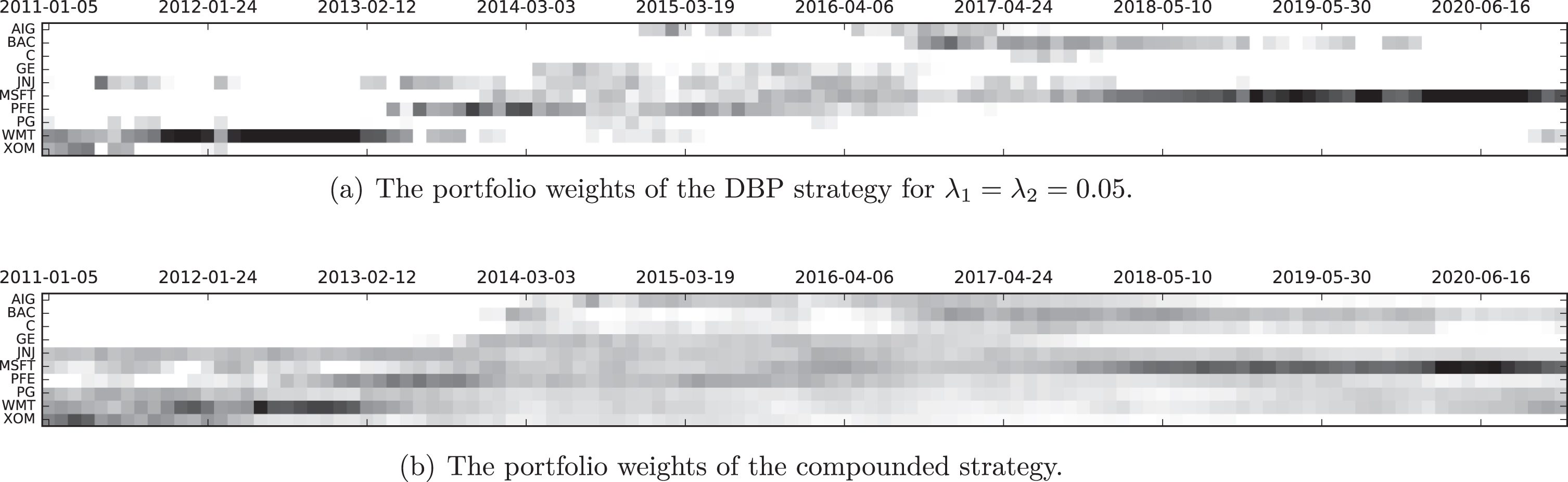
There are two benchmarks in the figure, the S&P 500 index, and a strategy that sets weights proportional to the compounded asset returns in the training dataset, where the weights of assets with negative returns are set to zero. We see that the discrepancy-based portfolio (DBP), obtained by solving the optimization problem (9), produces higher returns than these benchmarks. The Sharpe ratios of the strategies are: S&P 500: 0.7, compounded: 0.78, and DBP: 0.88. The instantaneous discrepancy d_t, and q_t variables for one training sample are shown in Figures 2(c) and 2(d), respectively. We see a batch of high discrepancy values around 2009, corresponding to the financial crisis, and that these dates have less weight in the optimization objective due to smaller or zero q_t values, as expected. In Figures 3(a) and 3(b) we plot portfolio weights, each time the portfolios are rebalanced, for the DBP and compounded strategies. We see that the temporal weight patterns of both strategies are similar, except that the DBP strategy produces portfolios that are more localized on the leading assets. This is understood since the algorithm is maximizing compounded returns rather than distributing weights proportional to individual asset performance, also recall that the solution of the linearized objective in w is a single asset.

Fig. 3

The portfolio weights of the of the DBP and compounded strategies, black is 1 and white is 0. We see that the weight-temporal patterns of both strategies are similar, except that the DBP strategy puts more weight on the leading assets.

6 Summary

We studied the problem of portfolio selection in non-stationary markets using a statistical learning approach. We bounded the generalization error of a non-stationary stochastic process by the sequential Rademacher complexity and the empirical discrepancy, and modified the bound for portfolio section by bounding the sequential Rademacher complexity. We used the learning bounds to obtain a sequential optimization algorithm for portfolio selection, and presented supportive numerical results with financial data.

Footnotes

Appendix

References

Adams,

T.M.

, Nobel,

A.B.

2010. Uniform convergence of vapnik–chervonenkis classes under ergodic sampling, Ann Probab38(4) 1345–1367.

Bertsekas,

1999. Nonlinear Programming, Athena Scientific.

Bogle,

J.C.

2017. The Little Book of Common Sense Investing, Wiley, 2nd edition.

Breiman,

2001. Statistical modeling: The two cultures, Statistical Science16(3), 199–231.

Cesa-Bianchi,

, Lugosi,

2006. Prediction, learning, and games., Cambridge University Press.

Cover,

T.M.

1991. Universal portfolios, Mathematical Finance1(1) 1–29.

Dehling,

, Mikosch,

, Sørensen,

2002. Empirical Process Techniques for Dependent Data, Birkhäuser Basel.

Hazan,

, Agarwal,

, Kale,

2007. Logarithmic regret algorithms for online convex optimization, Mach Learn69(2–3), 169–192.

Kuznetsov,

, Mohri,

2015. Learning theory and algorithms for forecasting non-stationary time series, in ‘Advances in Neural Information Processing Systems 28’, pp. 541–549.

10.

Kuznetsov,

, Mohri,

2020. Discrepancy-based theory and algorithms for forecasting non-stationary time series, Annals of Mathematics and Artificial Intelligence88(4), 367–399.

11.

Lee,

, Lee,

, Abbeel,

, Ng,

A.Y.

2006. Efficient l1 regularized logistic regression, in ‘In Proceedings of the Twenty-first National Conference on Artificial Intelligence (AAAI-06)’, pp. 1–9.

12.

Li,

, Hoi,

S.C.H.

2014. Online portfolio selection: A survey, ACM Comput Surv. 46(3).

13.

Mohri,

, Rostamizadeh,

2010. Stability bounds for stationary ϕ-mixing and β-mixing processes, J Mach Learn Res11, 789–814.

14.

Mohri,

, Rostamizadeh,

, Talwalkar,

2012. Foundations of Machine Learning, The MIT Press.

15.

Rakhlin,

, Sridharan,

2014. Statistical Learning and Sequential Prediction. Draft, chapter 10, available at http://www.mit.edu/ rakhlin/courses/stat928/stat928_notes.pdf.

16.

Rakhlin,

, Sridharan,

, Tewari,

2011. Online learning: Stochastic, constrained, and smoothed adversaries, in ‘Advances in Neural Information Processing Systems 24’, pp. 1764–1772.

17.

Rakhlin,

, Sridharan,

, Tewari,

2015a. Online learning via sequential complexities, Journal of Machine Learning Research16(6), 155–186.

18.

Rakhlin,

, Sridharan,

, Tewari,

2015b. Sequential complexities and uniform martingale laws of large numbers, Probability Theory and Related Fields161(1), 111–153.

19.

Wang,

, Carreira-Perpiñán,

2013. Projection onto the probability simplex: An efficient algorithm with a simple proof, and an application. Available at https://arxiv.org/abs/1309.1541.