Point-to-point stochastic control of a self-financing portfolio

Abstract

This paper aims at computing optimal control policies to drive a self-financing portfolio of financial assets from a given initial financial state to a final state in a given time horizon such that for the first case, the functional portfolio financial risk is minimized and, for the second case, the functional portfolio profit is maximized. The optimal control policies are the optimal investment allocation processes, the optimal state process is the optimal investor’s wealth process, also called the system response to the input control and is obtained by solving the combined system of differential equations formed by the state and costate system of differential equations derived and extracted from Pontryagin’s Minimum Principle. Computational simulations are provided to show the effectiveness and the reliability of the approach.

Keywords

Financial risk minimization Investment allocation optimal control portfolio construction portfolio optimization profit maximization self-financing portfolio stochastic differential equation

1 Introduction

Financial system dynamics involve considerable and significant randomness due to perturbation in the economic and political world. That’s why they are modelled by stochastic differential equations that enable researchers to rigorously analyse problems, solve them, and then interpret results to allow decision makers to prescribe reliable recommendations. Solving stochastic differential equations analytically is not easy. Consequently, the use of numerical methods is usually recommended. Financial operators and financial regulators in financial markets are mostly concerned with risk management and risk measurement to protect portfolios against random and harmful events. This article considers a self-financing portfolio with risk minimization and profit maximization. The study of portfolio dynamics is a critical topic in financial economics, financial engineering, financial mathematics, and in related areas. The control of self-financing portfolios is a relevant and critical issue that draws the attention of financial operators, financial managers, financial planners and financial regulators who have been dealing with similar and connected problems since some years. The literature defines a self-financing portfolio as one in which if there is no money coming in and no money moving out, then the purchase of a new financial asset is financed by the sale of an old one. Most of time the financial manager is concerned with maximizing the portfolio return and minimizing the portfolio risk which requires the use of Optimization and Optimal Control Theory techniques and tools. There exists a considerable body of research using Optimal Control Theory to rigorously and efficiently tackle financial optimization problems. Refer, for example, to Tomas (2010), Patrick and Ronnie (2016), Anton (2001), Li and Zhou (2006), Bielecki, Jin, PLiska and Zhou (2005) and Jiongming Yong and Xun Yu Zhou (1999). This paper aims to address, firstly, minimizing the self-financing integral functional portfolio risk, subject to the investor’s wealth dynamics and secondly, maximizing the integral functional portfolio expected profit subject to investor’s wealth dynamics; The wealth dynamics is described by a controlled stochastic differential equation, where the controls are the unknown investment allocation processes also called investment allocation policies which determine the instantaneous components of the portfolio. We are, firstly, dealing with a stochastic optimal control problem where the objective functional to minimize is the portfolio risk (defined by the portfolio variance), the control processes are the instantaneous investment allocation processes, the state process is the investor’s wealth process (where the wealth at the initial time is the capital). One of the papers in which is defined the wealth dynamics for the self-financing portfolio is Zhou and Li (2000). In such papers the wealth dynamics is left in terms of a stochastic differential equation. The authors optimized the portfolio at the final time. Unlike them, this paper solved the equation analytically and numerically and the portfolio is optimized over the whole time interval. In other words, this paper is concerned with computing the investment allocation processes to control the wealth dynamics at every point in time such that, firstly the functional risk is minimized, and secondly, the functional profit is maximized. The contributions (innovations) of this paper are the following:

Computation of the analytical and numerical solutions of the wealth equation. Indeed, the mean-variance presented by Markowitz constitutes a fundamental basis for portfolio optimization in a single period. It uses the variance to quantify the risk and offers to each financial operator the ability to maximize the portfolio expected return for an acceptable threshold of risk. The Markowitz theory did undergo some extensions. Zhou and Li (2000) used Markowitz theory as a starting point to maximize the return and minimize risk at the final time. The authors did transform their original optimal control problem into a class of auxiliary stochastic linear quadratic problems involving a stochastic Ricatti equation. This paper solved analytically and numerically, the original version of that equation.

Derivation of explicit numerical simulations of the wealth process in the self-financing portfolio by using successively and separately Euler-Maruyama, Milstein and Stochastic Runge-Kutta methods. For a judiciously provided control vector process, and depending on the researcher’s intuition and initiatives, each of the above numerical simulation can be coded into a function (or functions) to obtain numerical and computational solutions for the wealth stochastic differential equation. Since every derived numerical simulation concerns a stochastic model, it does not depend on the stationarity of the wealth time series, it then allows to obtain and forecast the value of wealth process as well as that of the financial portfolio process. Their solutions can be compared to the exact solution to assess their accuracies.

Approximation of the given controlled stochastic differential equation (the wealth equation) with a random ordinary differential equation. Such a trick enables the approximation of the Pontryagin Minimum Principle first-order necessary conditions for optimality (for the portfolio risk minimization problem) and the approximation of Pontryagin’s Maximum Principle first-order necessary conditions of optimality (for the portfolio profit maximization problem). Notice that the derivation of the first-order necessary conditions of optimality leads to the construction of the Hamiltonians systems, the computation, from the normal equations, of the control policy (Investment Allocation) processes in terms of the state (wealth) and costate (adjoint) processes. The expression of the control processes are substituted into the state and the costate system to judiciously vanish the unknown control and obtain everything in terms of only the state and costate processes.

As said above Zhou and Li (2000) minimize risk and maximize the expected return both at the final time. Unlike Zhou and Li (2000), this paper minimize the integral functional (whose integrand is the portfolio risk) and maximize the integral functional (whose integrand is the expected return) over the entire given time interval.

Development of computer programs consisting of interacting Matlab functions to solve the stochastic optimal control problem and obtain the control (investment allocation) processes, the state (wealth) process, the costate process, the Hamiltonian process, the risk process, the profit process, etc.

Computation of the numerical and computational portfolio risk (variance) process and the portfolio expected return process which are summarized by the associated computational simulations.

The paper is subdivided into the following sections: Section 2 presents the problem of portfolio risk minimization subject to wealth dynamics in the self-financing portfolio. Section 3 studies existence and uniqueness of solution of the wealth stochastic differential equation. Section 4 computes the analytical solution of the wealth equation. Section 5 derives, for a given control process, numerical simulation of the wealth equation by using successively numerical integration, Euler-Maruyama, Milstein, improved Euler-Maruyama, stochastic Runge-Kutta methods. Section 6 applies the Pontryagin Minimum principles of optimality to derive the Hamiltonian system containing differential equations involving random parameter for the state and the costate (adjoint) processes. Section 7 solves numerically the problem and obtain the optimal wealth (state) process which is the system response to the input control (investment allocation) processes, also called optimal state feedback control processes. The optimal investment allocation processes and the corresponding system response (which is the stochastic wealth process), are collectively called optimal pair, the stochastic costate process and the risk (variance) process are plotted to show the effectiveness of the approach and summarize the solutions. Section 8 presents the problem of portfolio profit maximization subject to wealth dynamics in the self-financing portfolio and suggests a method to find the solution. Section 9 concludes the paper by presenting the results and by discussing on them.

2 Portfolio risk minimization

The concern is to compute optimal investment allocation processes such that the functional portfolio risk is minimized. Such a problem is defined as follows:

$\begin{matrix} Minimize 𝔼 [J (ω)] & = & 𝔼 {\int_{0}^{T} \frac{1}{2} Ω Σ Ω dt} \\ = & 𝔼 {\int_{0}^{T} \frac{1}{2} \sum_{i = 1}^{N} \sum_{j = 1}^{N} ω_{i} σ_{ij} ω_{j} dt} \end{matrix}$ (1) subject to $\begin{matrix} dX (t) & = & {r (t) X (t) + \sum_{i = 1}^{m} [b_{i} (t) - r (t)] ω_{i}} dt \\ + \sum_{i = 1}^{m} \sum_{j = 1}^{m} σ_{ij} (t) ω_{i} (t) {dW}^{j} (t) \end{matrix}$ (2) $X (0) = X_{0} \geq 0$ (3) for t ∈ [0, T], where (1) is the running cost, the the functional portfolio risk defined by the portfolio variance, $\frac{1}{2} \sum_{i = 1}^{N} \sum_{j = 1}^{N} ω_{i} σ_{ij} ω_{j}$ is the rate of risk also called cost rate, Σ = (σ_i,j) _1≤i,j≤m is the covariance matrix for the portfolio financial risky asset profits (stocks), Ω = (ω₁ (t) , ..., ω_m (t)) is the risky portfolio where every component is a stochastic control process (investment allocation process), ω_i (t) is the investment allocation to the risky financial asset i at time t, {X (t)} _t≥0 is the stochastic state process, the investor’s stochastic wealth process, b_i (t) is the appreciation rate of portfolio stock i at time t, it is also called growth rate, r (t) is portfolio bond interest rate at time t, it is also called the bond growth rate, σ_ij (t) is the covariance between asset i and asset j at time t. From a stochastic control point of view, X (t) _t≥0 and ω_i (t) _{i=1,...,N t≥0} are respectively the unknown state stochastic process and stochastic control processes for the asset i at time t. The control processes constitute the investor’s portfolio stochastic process. By definition, a stochastic process is a finite or an infinite sequence (X_t = X (t)) _t≥0 such that at every time t ≥ 0, X_t is a random variable.

The investment allocation for asset i is given by:

$ω_{i} (t) = N_{i} (t) P_{i} (t) \forall i = 1, \dots, m .$ (4) where N_i (t) and P_i (t) are respectively the number of shares and the market value (price) for the risky asset (stock) number i at time t where the asset price P_i (t) follows the following stochastic process:

$\begin{matrix} {dP}_{i} (t) & = & P_{i} (t) {b_{i} (t) dt + \sum_{j = 1}^{m} σ_{ij} (t) {dW}_{j} (t)}, \\ i = 1, \dots, m \end{matrix}$ (5) For the riskless asset (bond) there is no stochastic component, then the equation is as follows:

${dP}_{0} (t) = {rP}_{0} (t) dt$ (6) where r is the growth rate for the bond whose price at time t is P₀ (t). The wealth X (t) is given by:

$X (t) = \sum_{i = 1}^{m} ω_{i} (t) = \sum_{i = 1}^{m} N_{i} (t) P_{i} (t)$ (7) At time t = 0, the wealth X (0)is called the capital. At that time the investment allocation (portfolio selection) problem is also called “Capital Budgeting” problem. The change in the wealth is:

$dX (t) = \sum_{i = 0}^{m} N_{i} (t) {dP}_{i} (t)$ (8)

3 Existence and uniqueness of solution

Redefine equation (2) in terms of functions f (.) and g (.) (which are respectively its drift and its diffusion coefficients) so that we can be able to address concisely and in compact way the existence and uniqueness of solution. We then have the following:

$\begin{matrix} f (t, X (t), ω_{1} (t), \dots, ω_{m} (t)) \\ = r (t) X (t) + \sum_{i = 1}^{m} [b_{i} (t) - r (t)] ω_{i} \end{matrix}$ (9) and

$\begin{matrix} g (t, X (t), ω_{1} (t), \dots, ω_{m} (t)) \\ = Σ (t) Ω (t) = \sum_{i = 1}^{m} \sum_{j = 1}^{m} σ_{ij} (t) ω_{i} (t) \end{matrix}$ (10) Then, the wealth equation (2) can be rewritten as:

$\begin{matrix} dX (t) & = & f (t, X (t), ω_{1} (t), \dots, ω_{m} (t)) dt \\ + g (t, (t), ω_{1} (t), \dots, ω_{m} (t)) dW \end{matrix}$ (11) From Ito calculus point of view, f (t, X (t) , ω₁ (t) , ..., ω_m (t)) and g (t, X (t) , ω₁ (t) , ..., ω_m (t))are the drift rate and the diffusion rate of the wealth. The equation admits a solution because for any given Wiener process {W (t)} _t≥0 and any feasible input control processes (ω₁ (t) , ..., ω_m (t)) , f (t, X (t) , ω₁ (t) , ..., ω_m (t)) and g (t, X (t) , ω₁ (t) , ..., ω_m (t)) are clearly and sufficiently continuous with respect to their arguments.

The solution is unique because function f (t, X (t) , ω₁ (t) , ..., ω_m (t)) and function g (t, X (t) , ω₁ (t) , ..., ω_m (t)) satisfy the Lipschitz condition. For any details on Lipschitz condition, the reader is kindly referred to articles and books on analytical and numerical solution of differential equations.

4 Computation of analytical solution of the SDE

Reconsider the controlled stochastic differential equation. $\begin{matrix} dX (t) & = & {r (t) X (t) + \sum_{i = 1}^{m} [b_{i} (t) - r (t)] ω_{i} (t)} dt \\ + \sum_{i = 1}^{m} \sum_{j = 1}^{m} σ_{ij} (t) ω_{i} (t) {dW}_{t}^{j} \end{matrix}$ (12) $X (0) = X_{0} \geq 0$ (13) It is clear that the coefficient of dt and the coefficients of dW^j are continuous with respect to their arguments and satisfy Lipschitz condition. Then, for any given Wiener process {W (t)} _t≥0 and any feasible input control processes (ω₁ (t) , ..., ω_m (t)), the solution exists, is unique and is a stochastic process X (t) _t≥0. The above stochastic differential equation can be explicitly solved since it is linear. It satisfies the following general form of stochastic differential equations:

$\begin{matrix} dX (t) & = & (a (t) X (t) + c (t)) dt + (b (t) X (t) \\ + d (t)) dW (t) \end{matrix}$ (14) Which has the solution

$\begin{matrix} X (t) & = & Φ_{t, t_{0}} (X (t_{0}) + \int_{t_{0}}^{t} Φ_{s, t_{0}}^{- 1} (c (s) - b (s) d (s)) ds \\ + \int_{t_{0}}^{t} Φ_{s, t_{0}} d (s)) dW (s)) \end{matrix}$ (15) Where

$\begin{matrix} Φ_{t, t_{0}} & = & \exp (\int_{t_{0}}^{t} (a (s) - \frac{b^{2} (s)}{2}) ds + \int_{t_{0}}^{t} b (s) dW (s)) \end{matrix}$ (16) By comparing equations (12) and (14) we have that $a (t) = r (t)$ (17) $c (t) = \sum_{i = 1}^{m} [b_{i} (t) - r (t)] ω_{i} (t)$ (18) $b (t) = 0$ (19) $d_{j} (t) = 0 \forall j = 1, \dots, m .$ (20) $d (t) = (d_{1} (t), \dots, d_{m} (t)) where$ (21) $\begin{matrix} d_{j} (t) & = & σ_{1 j} ω_{1} + σ_{2 j} ω_{2} + \dots + σ_{kj} ω_{k} \\ + \dots + σ_{mj} ω_{m} \end{matrix}$ (22) Therefore, the analytical solution of equation (12) is given as:

$\begin{matrix} X (t) & = & Φ_{t, 0} (X (0) + \int_{0}^{t} Φ_{s, 0}^{- 1} \sum_{i = 1}^{m} \\ [b_{i} (s) - r (s)] ω_{i} (s) ds \\ + \sum_{j = 1}^{m} \int_{0}^{t} Φ_{s, 0}^{- 1} d_{j} (s) {dW}_{s}^{j}) \end{matrix}$ (23) Where

$\begin{matrix} d_{j} (t) & = & σ_{1 j} ω_{1} + σ_{2 j} ω_{2} + \dots + σ_{kj} ω_{k} \\ + \dots + σ_{mj} ω_{m} \forall j = 1, \dots, m \end{matrix}$ (24)

5 Computation of numerical solutions of the SDE

Reconsider the above equation (2) defining the wealth dynamics. For an imposed or a provided optimal input control process Ω = (ω₁ (t) , ..., ω_m (t)), the numerical solution, also called the optimal system response (the optimal wealth) is as follows:

$\begin{matrix} X (t) & = & X (0) + \int_{0}^{t} {r (s) X (s) \\ + \sum_{i = 1}^{m} [b_{i} (s) - r (s)] ω_{i}} ds \\ + \int_{0}^{t} \sum_{i, j = 0}^{m} σ_{ij} (s) ω_{i} (s) {dW}_{s}^{j} \end{matrix}$ (25) where $\int_{0}^{T} \sum_{i, j = 0}^{m} σ_{ij} (s) ω_{i} (s) {dW}_{s}^{j} = \int_{0}^{T} \sum_{i, j = 0}^{m} σ_{ij} (s) ω_{i} (s) {dW}^{j} (s)$ is called the Ito integral. We obviously have that

$\int_{0}^{t} {r (s) X (s) + \sum_{i = 0}^{m} [b_{i} (s) - r (s)] ω_{i}} ds < \infty$ (26) and

$\int_{0}^{t} \sum_{i, j = 0}^{m} σ_{ij} (s) ω_{i} (s) {dW}_{s}^{j} < \infty$ (27) Then, the solution defined by the expression (25) exists and that at every t ∈ [0, T] and it can be computed analytically and / or numerically.

Divide the given time interval [0, T] into N subintervals 0 = t₀ < t₁ < ... < t_N = T where $h = Δ t_{i} = t_{i + 1} - t_{i} = \frac{T}{N}$ and $Δ W_{i}^{j} = W_{i + 1}^{j} - W_{i}^{j} = Z_{i}^{j} \sqrt{Δ t_{i}}$ (where for practical applications $Z_{i}^{j}$ is generated randomly) and let Y_i = X (t_i).

5.1 Numerical simulation of the state (wealth) stochastic differential equation using Euler-Maruyama method

By applying the Euler-Maruyama numerical method to solve the given wealth equation (2), provided a Wiener process {W (t)} _t≥0 discretized into {W_kk≥0 and any feasible input control processes (ω₁ (t) , ..., ω_m (t)), discretized into (ω_1,k, ..., ω_m,k) one finds the approximate solution given as follows: $\begin{matrix} Y_{0} & = & X_{0} \\ Y_{k + 1} & = & Y_{k} + {r_{k} Y_{k} + \sum_{i = 0}^{m} [b_{i, k} - r_{k}] ω_{i, k}} Δ t_{k} + \sum_{i, j = 0}^{m} σ_{ij, k} ω_{i, k} Δ W_{k}^{i} \end{matrix}$ (28) where b_i,k = b_i (t_k)is the appreciation rate of stock i at time t_k, r_k = r (t_k), is the interest rate of the bond at time t_k, Y_k, is the approximate value of the wealth Y (t_k)at time t_k, $Δ W_{k}^{i} = W_{k + 1}^{i} - W_{k}^{i}$ is the approximate value of ΔWⁱ (t_k). It is the change between two random variables of a Wiener process. By using equation (7), (28) is simplified as follows:

$\begin{matrix} Y_{0} & = & X_{0} \\ Y_{k + 1} & = & Y_{k} + Δ t_{k} \sum_{i = 0}^{m} b_{i, k} ω_{i, k} + \sum_{i, j = 0}^{m} σ_{ij, k} ω_{i, k} Δ W_{k}^{i} \end{matrix}$ (29)

For some optimal input control processes judiciously designed, one can kindly compute and obtain the investor’s optimal wealth process.

5.2 Numerical simulation of the state (wealth) stochastic differential equation by using milstein method

By using the Milstein numerical simulation, the approximate solution to the stochastic differential equation (2) is the following:

$\begin{matrix} Y_{0} & = & X_{0} \\ Y_{k + 1} & = & Y_{k} + {r_{k} Y_{k} + \sum_{i = 0}^{m} [b_{i, k} - r_{k}] ω_{i, k}} Δ t_{k} + b (Y_{k}, t_{k}) Δ W_{k}^{i} + \frac{1}{2} b (Y_{k}, t_{k}) \frac{\partial b}{\partial X} (Y_{k}, t_{k}) (Δ W_{k}^{i 2} - Δ t_{k}) \end{matrix}$ (30) By using equation (7), (30) is simplified as follows:

$\begin{matrix} Y_{0} & = & X_{0} \\ Y_{k + 1} & = & Y_{k} + Δ t_{k} \sum_{i = 0}^{m} b_{i, k} ω_{i, k} + b (Y_{k}, t_{k}) Δ W_{k}^{i} + \frac{1}{2} b (Y_{k}, t_{k}) \frac{\partial b}{\partial X} (Y_{k}, t_{k}) (Δ W_{k}^{i 2} - Δ t_{k}) \end{matrix}$ (31) For an optimal input control processes judiciously designed, one can kindly compute and obtain the investor’s optimal wealth process.

5.3 Numerical simulation using an improved euler method

Consider the wealth equation (2) as rewritten in compact form by (11). The numerical solution is given by:

$\begin{matrix} X (0) & = & X_{0} \\ K_{1} & = & hf (t_{k}, X_{k}, ω_{1, k}, \dots, ω_{m, k}) + (Δ W_{k} - S_{k} \sqrt{h}) g (t_{k}, X_{k}, ω_{1, k}, \dots, ω_{m, k}) \\ K_{2} & = & hf (t_{k + 1}, X_{k} + K_{1}, ω_{1, k}, \dots, ω_{m, k}) + (Δ W_{k} + S_{k} \sqrt{h}) g (t_{k + 1}, X_{k} + K_{1}, ω_{1, k}, \dots, ω_{m, k}) \\ X_{k + 1} & = & X_{k} + \frac{1}{2} (K_{1} + K_{2}) \end{matrix}$ (32) where $Δ W_{k} = \sqrt{h} Z_{k}$ for normal random Z_k ≈ N (0, 1)and S_k = + -1. Each alternative chosen with probability 0.5

5.4 Numerical simulation using Runge-Kutta method

Consider the wealth equation (2) as rewritten in compact form by (11). Then the Runge Kutta numerical simulation of the wealth stochastic differential equation is as follows:

$\begin{matrix} Y_{i} & = & y_{n} + h \sum_{j = 1}^{s} a_{ij} f (t_{j}, Y_{j}, ω_{1} (t), \dots, ω_{m} (t)) \\ + J_{1} \sum_{j = 1}^{s} b_{ij} g (t_{j}, Y_{j}, ω_{1} (t), \dots, ω_{m} (t)) \end{matrix}$ (33)

$\begin{matrix} y_{n + 1} & = & y_{n} + h \sum_{j = 1}^{s} α_{i} f (t_{j}, Y_{j}, ω_{1} (t), \dots, ω_{m} (t)) \\ + J_{1} \sum_{j = 1}^{s} γ_{j} g (t_{j}, Y_{j}, ω_{1} (t), \dots, ω_{m} (t)) \end{matrix}$ (34)

where A = (a_ij)andB = (b_ij)ares * s real matrices, α^T = (α₁, ..., α_s) are now vectors belonging to R. Runge-Kutta numerical simulation may be used to approximate, for a judiciously designed and provided control processes (Investment Allocations), compute the numerical solution of the wealth equation. For each of the above considered numerical simulation method, for a designed optimal control policy, the solution to the stochastic differential equation (2) is the optimal wealth for the investor.

where $b = Σ Ω = (\sum_{i, j = 0}^{m} σ_{ij} (t) ω_{i} (t))_{1 \leq i \leq m}$ is a vector, $b (Y_{i}, t_{i}) Δ W_{i} = \sum_{i, j = 0}^{m} σ_{ij} (t) ω_{i} (t) {dW}^{j} (t)$ Σ = (σ_i,j) _1≤i,j≤morder m , Ω = (ω₁, ..., ω_m)is a vector of the proportions to be held in the portfolio, W = (W₁, ..., W_m), Δt_i = t_i+1 - t_i and $Δ W_{i}^{j} = W_{i + 1}^{j} - W_{i}^{j}$ , i refer to time and j refer to a stock, ${W_{i}^{j}, i = 1, \dots, N and, j = 1, \dots, N}$ is a discrete stochastic process in which $W_{i}^{j}$ is a discrete random variable related to stock number j at time i. By dividing the left hand side and the right hand side of equation (2) by dt and by letting

$Θ_{j} (t) = \frac{{dW}_{j}}{dt} (t)$ , then the above problem (1)-(2)can be approximately reformulated as follows:

$\begin{matrix} Minimize 𝔼 [J (ω)] = 𝔼 {\int_{0}^{T} \frac{1}{2} Ω Σ Ω dt} \\ = 𝔼 {\int_{0}^{T} \frac{1}{2} \sum_{i = 1}^{N} \sum_{j = 1}^{N} ω_{i} σ_{ij} ω_{j} dt} \end{matrix}$ (35) subject to $\begin{matrix} \frac{dX}{dt} (t) & = & {r (t) X (t) + \sum_{i = 1}^{m} [b_{i} (t) - r (t)] ω_{i} (t)} \\ + \sum_{j = 1}^{m} \sum_{i = 1}^{m} σ_{ij} (t) ω_{i} (t) Θ_{j} (t) \end{matrix}$ (36) $X (0) = X_{0} > 0$ (37) Equation (36) expresses the rate of change of total investor’s wealth.

6 Auxiliary optimal control problem

Let Ω₀ denotes the set of control processes as above defined,

$U_{0} = {ω_{i} \in R : ω_{i} = N_{i} P_{i}} .$ (38) Let U denotes the set of all piecewise continuous control processes ω_i ∈ Ω₀, t ∈ [0, T].

The feasible control problem is formulated as follows: Given an initial wealth X (0) = X₀ ∈ R, compute a control vector process strategy ω (·) ∈ U to bring the system (36) from the specified initial state to a certain free X (T) final state such that the portfolio risk is minimized. This stochastic control strategy will be called a feasible control process strategy, feasible investment allocation processes.

Define the auxiliary optimal control problem such that the computation of a feasible control approximating the optimal control can be achieved. Numerical and computational methods are expected to be used to obtain the results.

The Hamiltonian function is given by:

$\begin{matrix} H (t, X, ω_{1}, \dots, ω_{m}, λ) \\ = L (t, X, ω_{1}, \dots, ω_{m}) - λ f (t, X, ω_{1}, \dots, ω_{m}) . \end{matrix}$ (39) where

$L (t, X, ω_{1}, \dots, ω_{m}) = \frac{1}{2} \sum_{i = 1}^{m} \sum_{j = 1}^{m} ω_{i} σ_{ij} ω_{j}$ (40)

$\begin{matrix} f (t, X, ω_{1}, \dots, ω_{m}) & = r (t) X (t) + \sum_{i = 0}^{m} [b_{i} (t) - r (t)] ω_{i} \\ + \sum_{j = 0}^{m} \sum_{i = 0}^{m} σ_{ij} (t) ω_{i} (t) Θ_{j} (t) \end{matrix}$ (41)

To compute Ω = (ω₁ (t) , ..., ω_m (t)), first calculate the following expressions:

$\begin{matrix} \frac{\partial H}{\partial ω_{1}} & = & \sum_{j = 1}^{m} σ_{1 j} ω_{j} - λ {(b_{1} - r) + \sum_{j = 1}^{m} σ_{1 j} Θ_{j}} \\ \frac{\partial H}{\partial ω_{2}} & = & \sum_{j = 1}^{m} σ_{2 j} ω_{j} - λ {(b_{2} - r) + \sum_{j = 1}^{m} σ_{2 j} Θ_{j}} \\ ⋮ & ⋮ & ⋮ \\ \frac{\partial H}{\partial ω_{k}} & = & \sum_{j = 1}^{m} σ_{kj} ω_{j} - λ {(b_{k} - r) + \sum_{j = 1}^{m} σ_{kj} Θ_{j}} \\ ⋮ & ⋮ & ⋮ \\ \frac{\partial H}{\partial ω_{m - 1}} & = & \sum_{j = 1}^{m} σ_{m - 1, j} ω_{j} - λ {(b_{m - 1} - r) + \sum_{j = 1}^{m} σ_{m - 1, j} Θ_{j}} \\ ∥ \frac{\partial H}{\partial ω_{m}} & = & \sum_{j = 1}^{m} σ_{mj} ω_{j} - λ {(b_{m} - r) + \sum_{j = 1}^{m} σ_{mj} Θ_{j}} \end{matrix}$ (42)

The first-order optimality conditions, ∀i = 1, ..., m let $\frac{\partial H}{\partial ω_{i}} = 0$ , lead to the following linear system of equations (where the unknowns are ω₁, ..., ω_m):

$\begin{matrix} \sum_{j = 1}^{m} σ_{1 j} ω_{j} & = & λ {(b_{1} - r) + \sum_{j = 1, j \neq 1}^{m} σ_{1 j} Θ_{j}} \\ \sum_{j = 1}^{m} σ_{2 j} ω_{j} & = & λ {(b_{2} - r) + \sum_{j = 1, j \neq 2}^{m} σ_{2 j} Θ_{j}} \\ ⋮ & ⋮ & ⋮ \\ \sum_{j = 1}^{m} σ_{kj} ω_{j} & = & λ {(b_{k} - r) + \sum_{j = 1, j \neq k}^{m} σ_{kj} Θ_{j}} \\ ⋮ & ⋮ & ⋮ \\ \sum_{j = 1}^{m} σ_{m - 1, j} ω_{j} & = & λ {(b_{m - 1} - r) + \sum_{j = 1, j \neq m - 1}^{m} σ_{m - 1, j} Θ_{j}} \\ ∥ \sum_{j = 1}^{m} σ_{mj} ω_{j} & = & λ {(b_{m} - r) + \sum_{j = 1, j \neq m}^{m} σ_{mj} Θ_{j}} \end{matrix}$ (43)

which can be rewritten in matrix form as:

$\begin{matrix} [\begin{matrix} σ_{11} & σ_{12} & \dots & σ_{1 m} \\ σ_{21} & σ_{22} & \dots & σ_{2 m} \\ ⋮ & ⋮ & ⋱ & ⋮ \\ σ_{k 1} & σ_{k 2} & \dots & σ_{km} \\ ⋮ & ⋮ & ⋱ & ⋮ \\ σ_{m 1} & σ_{m 2} & \dots & σ_{mm} \end{matrix}] [\begin{matrix} ω_{1} \\ ω_{2} \\ ⋮ \\ ω_{m} \end{matrix}] \\ = λ [\begin{matrix} b_{1} - r \\ b_{2} - r \\ ⋮ \\ b_{m} - r \end{matrix}] + [\begin{matrix} σ_{11} & σ_{12} & \dots & σ_{1 m} \\ σ_{21} & σ_{22} & \dots & σ_{2 m} \\ ⋮ & ⋮ & ⋱ & ⋮ \\ σ_{k 1} & σ_{k 2} & \dots & σ_{km} \\ ⋮ & ⋮ & ⋱ & ⋮ \\ σ_{m 1} & σ_{m 2} & \dots & σ_{mm} \end{matrix}] [\begin{matrix} Θ_{1} \\ Θ_{2} \\ ⋮ \\ Θ_{m} \end{matrix}] \end{matrix}$ (44) By letting $Σ = [\begin{matrix} σ_{11} & σ_{12} & \dots & σ_{1 m} \\ σ_{21} & σ_{22} & \dots & σ_{2 m} \\ ⋮ & ⋮ & ⋱ & ⋮ \\ σ_{k 1} & σ_{k 2} & \dots & σ_{km} \\ ⋮ & ⋮ & ⋱ & ⋮ \\ σ_{m 1} & σ_{m 2} & \dots & σ_{mm} \end{matrix}]$ , $Ω = [\begin{matrix} ω_{1} \\ ω_{2} \\ ⋮ \\ ω_{m} \end{matrix}]$ , $b = [\begin{matrix} b_{1} \\ b_{2} \\ ⋮ \\ b_{m} \end{matrix}]$ and $Θ = [\begin{matrix} Θ_{1} \\ Θ_{2} \\ ⋮ \\ Θ_{m} \end{matrix}]$ , the system can be rewritten as:

$Σ Ω = λ (B - rI) + Σ Θ$ (45) and then we find the value of Ω as

$Ω = λ Σ^{- 1} (B - rI) + Θ$ (46) where r ≥ 0, λ ∈ R, I is a column vector of the same size as B and that contains one everywhere. Ω, Σ and Θ are as above specified. Therefore we have

$Ω = λ Σ^{- 1} (B - rI) + Θ$ (47) Given an initial condition of the system X (0) = X₀, consider the risk functional J given by (1), consider the problem of computing a control ω (·) ∈ U for the wealth stochastic system such that J is minimized. By applying Pontryagin Minimum Principle Victor Emmanuel Becerra (2004), Dimitri P. Bertsekas (2000) and Jiongming Yong & Xun Yu Zhou (1999), the following is implied:

Since $Ω^{*} (t) = (ω_{1}^{*}, \dots, ω_{m}^{*}) \in U_{0}, t \in [0, T]$ is the optimal stochastic control process (the optimal investment allocation process strategies) for the above problem and X^* (t) , t ∈ [0, T] is the corresponding system response stochastic process, then there exists a function λ^* (t) , t ∈ [0, T], called the costate (or adjoint) process, such that the following equations are satisfied:

$\begin{matrix} Ω^{*} & = & (ω_{1}^{*}, \dots, ω_{m}^{*}) = λ^{*} Σ^{- 1 *} (B - rI) + Θ^{*} \end{matrix}$ (48)

$\begin{matrix} \frac{{dX}^{*}}{dt} (t) & = & r (t) X^{*} (t) + \sum_{i = 0}^{m} [b_{i} (t) - r (t)] ω_{i}^{*} \\ + \sum_{j = 0}^{m} \sum_{i = 0}^{m} σ_{ij} (t) ω_{i}^{*} (t) Θ_{j} (t) \end{matrix}$ (49)

$X^{*} (0) = X_{0}^{*} \geq 0$ (50)

$\frac{d λ^{*}}{dt} (t) = r (t) λ^{*} (t), λ^{*} (0) = λ_{0}^{*}$ (51)

7 Computational simulations

The equations (48) – (51) state Pontryagin’s Minimum Principle of optimality. Such equations form a system of equations which is solved using a fourth-order Runge-Kutta method.

For the inputs, numerical data for the stocks were randomly generated three times to show the effectiveness of the approach. For the first case, random data were generated as six time series for the stock returns where every time series has a hundred elements. Every time series gives a stock profile from time t = 1to timet = 100. From those time series a covariance matrix was computed to show the correlation between stocks. Such a covariance matrix serves as input for the objective functional represented by the risk function which is the variance of the portfolio profit. Such a function also involves the unknown investment allocations representing the stochastic control processes. Some elements of the covariance matrix are also needed in the diffusion component of the wealth equation. After solving the system of equations representing Pontriagin’s Minimum Principle of optimality we obtain the stochastic control processes which constitute the portfolio stock investment allocations given in Figure 1. At every time tthere is an investment allocation. From the second plot of Figure 1, the reader can notice that the second function is zero at every time which instructs the investor to allocate nothing to the associated stock (stock number 2) during the considered time interval. Money will be allocated only to stocks number 1, 3, 4, 5 and 6 according to the results in the plots. Such stocks will constitute the portfolio. The amount of investment to allocate for a stock depends on the performance of the associated stock. The better it performs, the greater is the amount allocated. Then, the system state response (also called the wealth) to the input control processes, and the associated costate process (also called adjoint process), are obtained. This is shown in Figure 2 and Figure 3, respectively where one can notice that the wealth is increasing.

Fig. 1

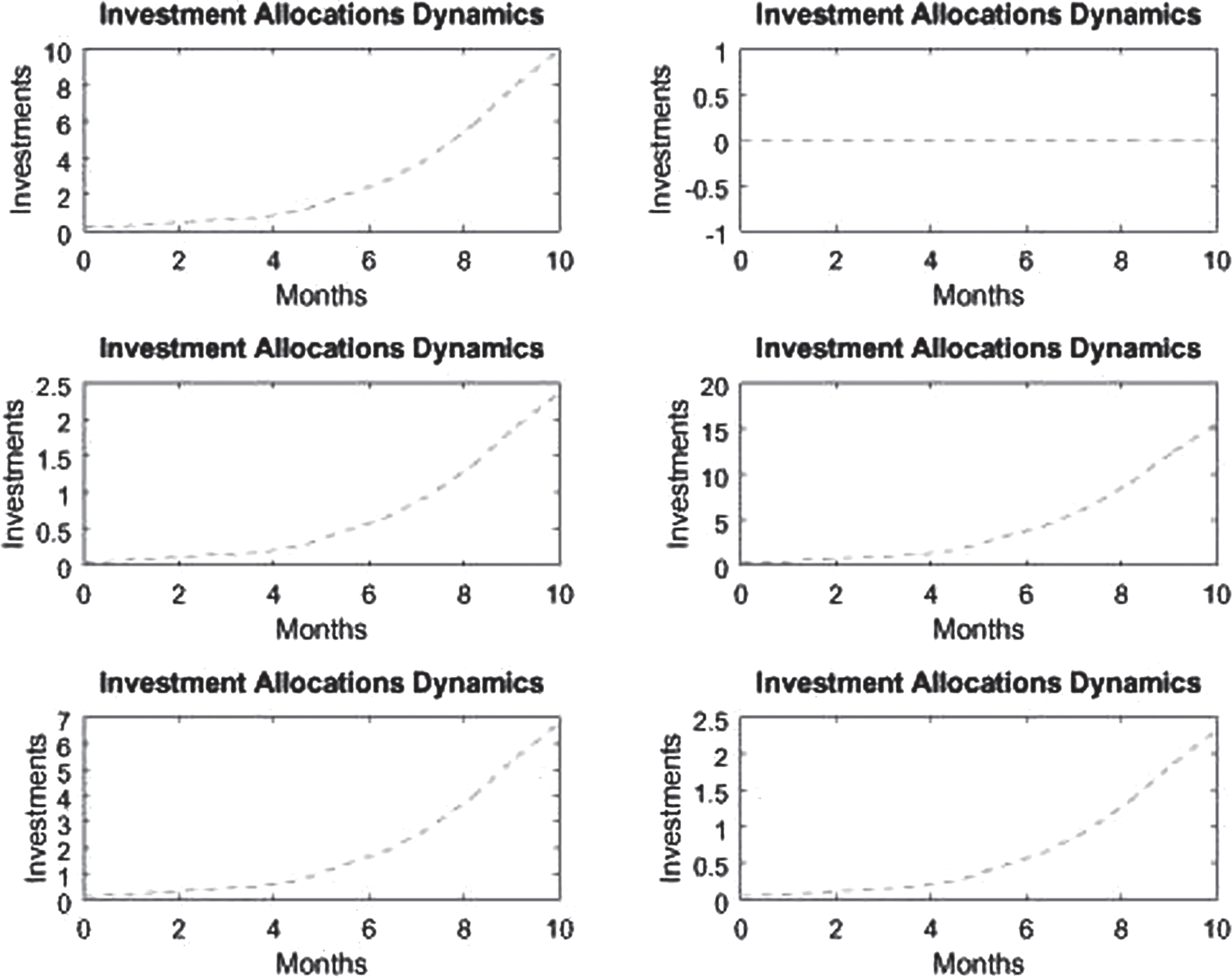
Plot of the Portfolio Stock Investment allocations.

Fig. 2

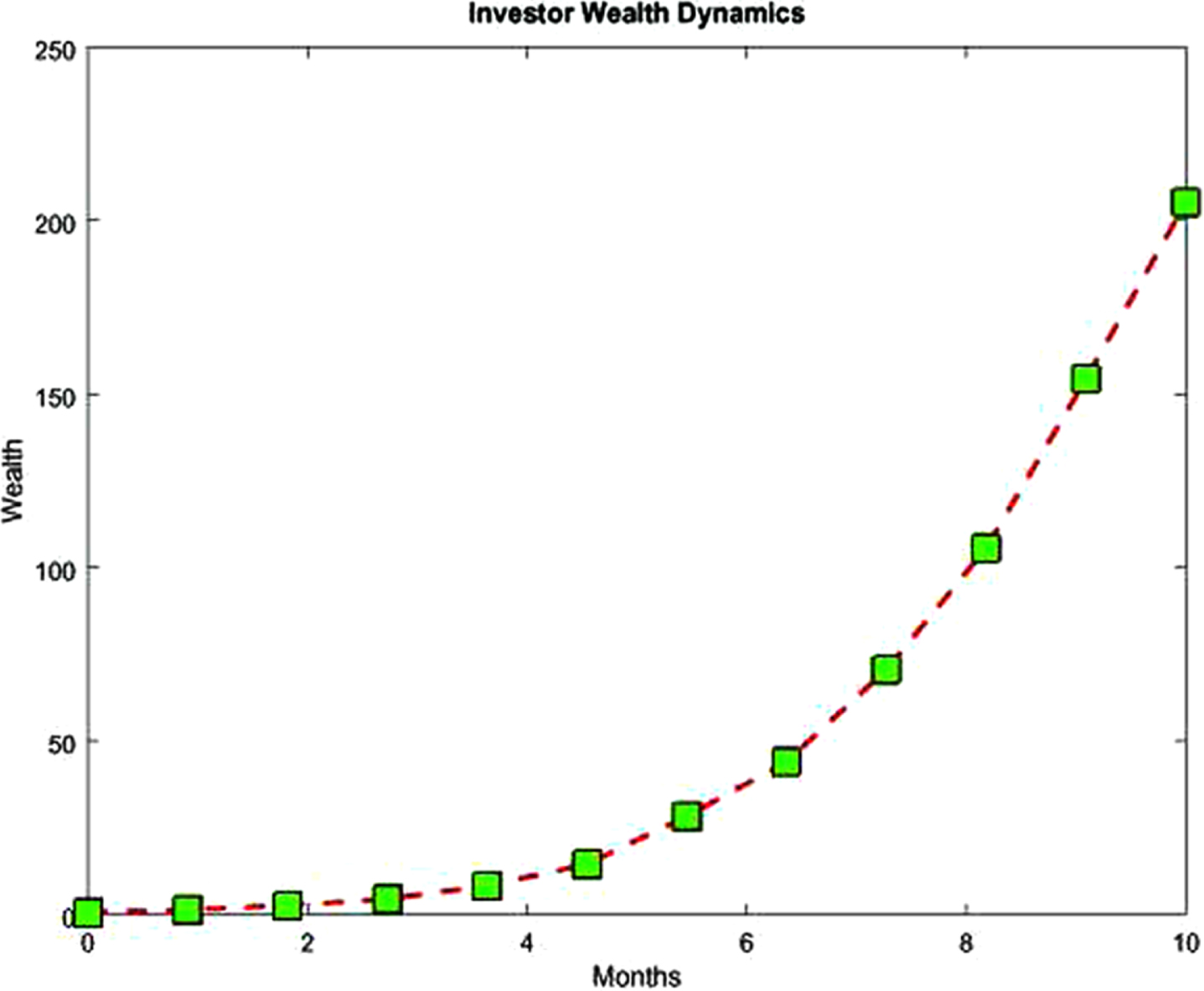
Plot of Wealth versus Time.

Fig. 3

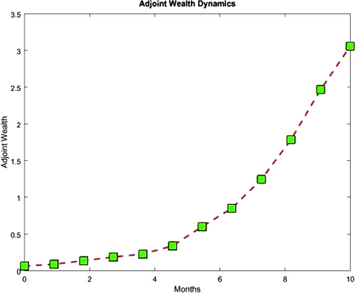
Plot of the costate process.

As in the first case, the same procedure is performed in the second case, and yields the input control processes which are the stock investment allocations as shown in Figure 4. One will notice that there is nothing to allocate to stock number 1, 2 and 5 during the considered time interval since their associated investment allocation functions are zero at every time. The portfolio is only constituted by stocks 3, 4 and 6 from the first month to the last. Then, the related system response, and its adjoint, are shown in Figure 5 and Figure 6 respectively. Again, the wealth is increasing. The risk (variance) is plotted and represented in Figure 7 which shows a considerable, significant and reliable risk minimization.

Fig. 4

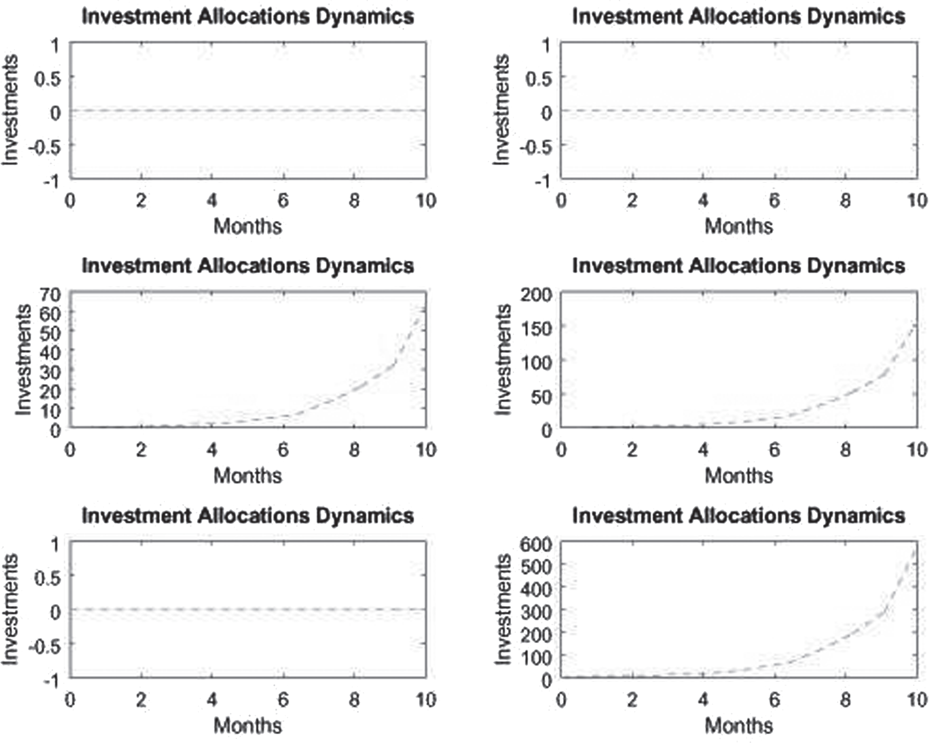
Plot of the Portfolio Stock Investment allocations.

Fig. 5

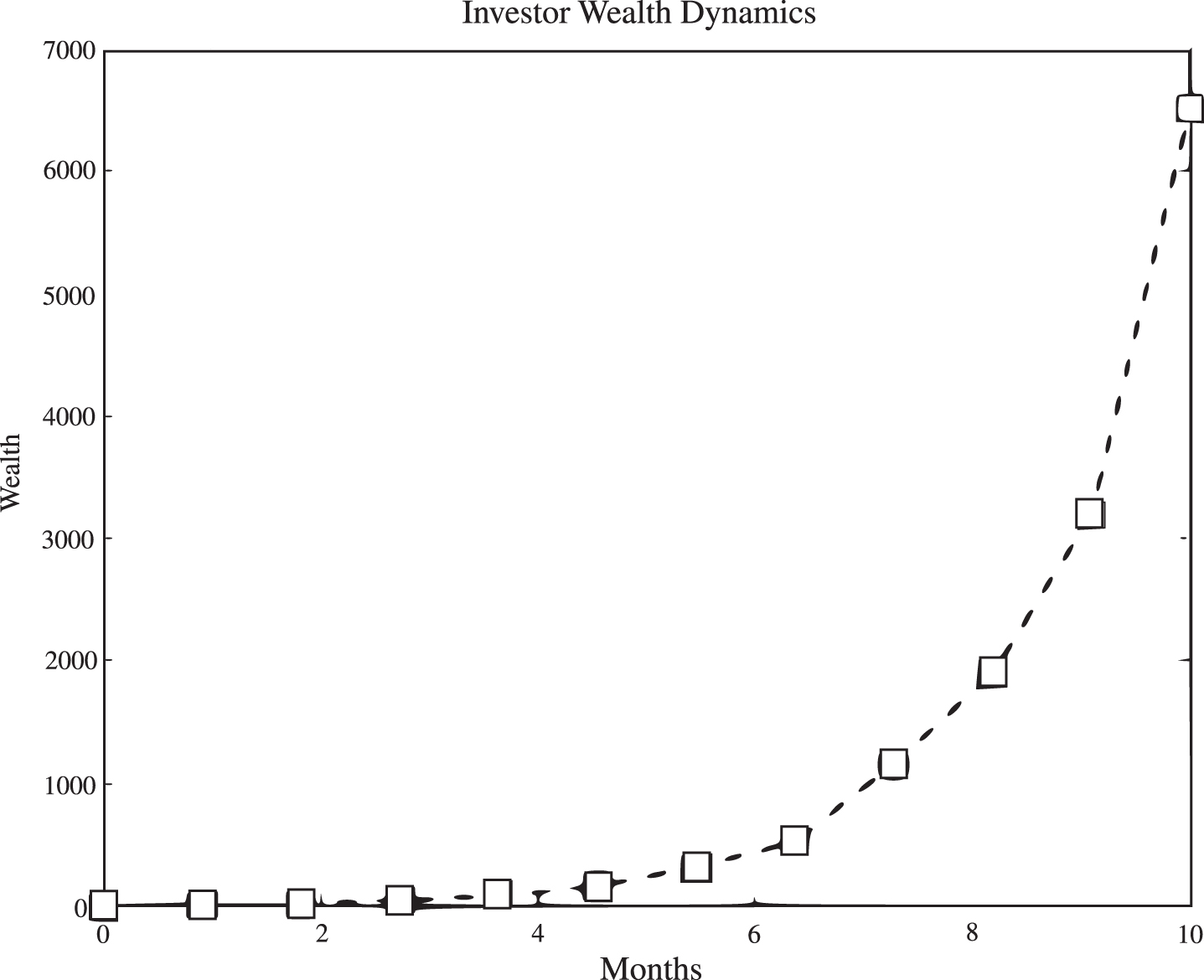
Plot of Wealth versus Time.

Fig. 6

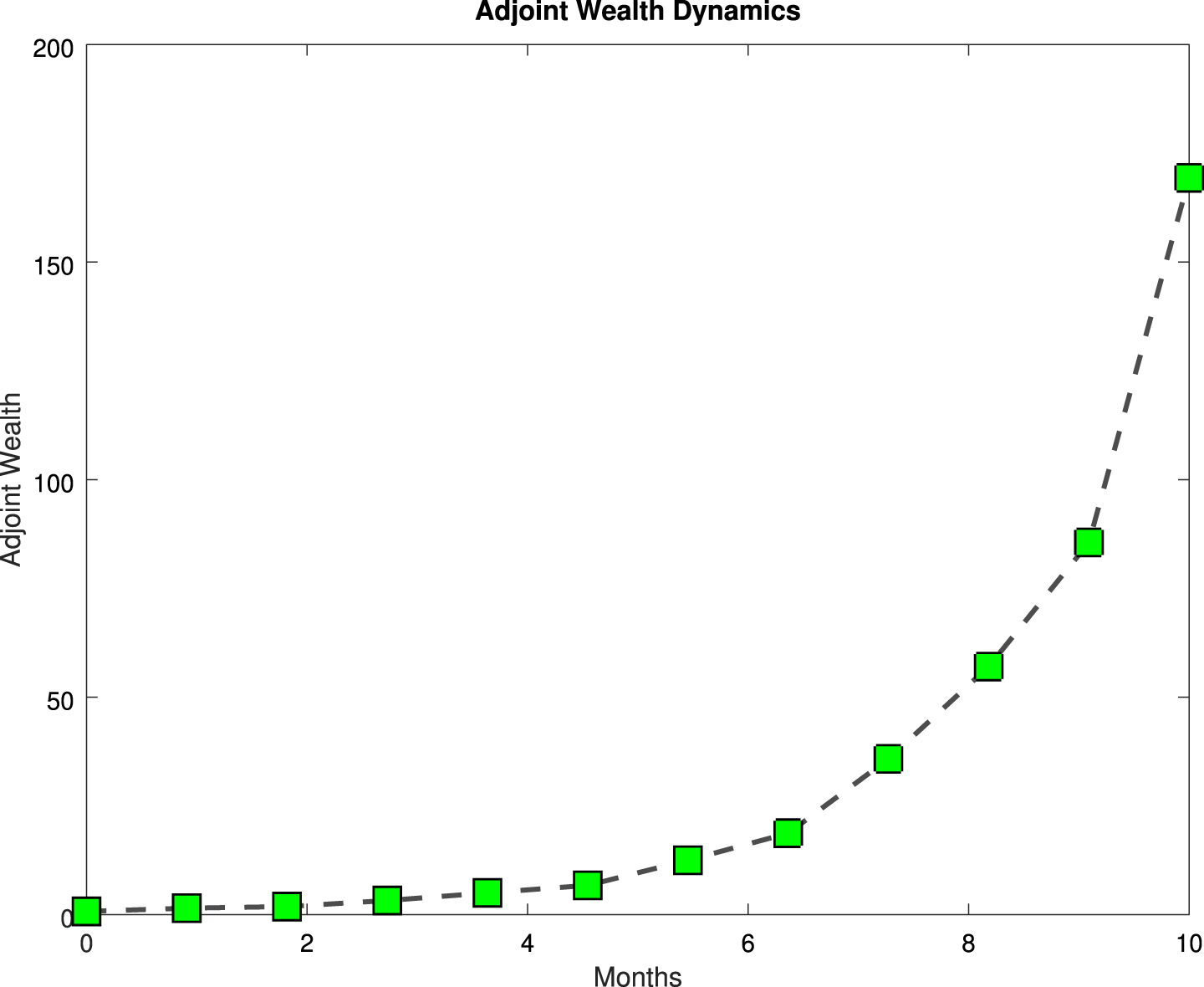
Plot of the costate process related to the wealth process.

Fig. 7

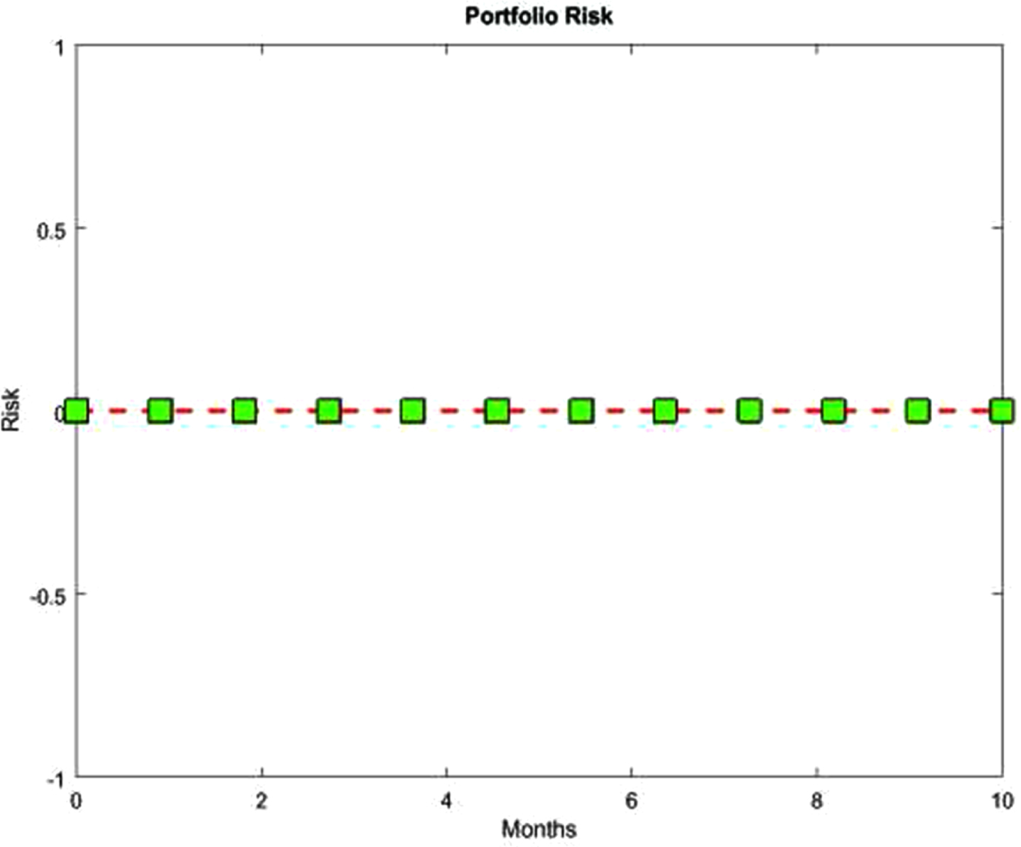
Plot of risk versus Time.

As for the two previous cases, the third case shows that the generated input data to the optimal control problem together with Pontryagin’s Minimum Principle gives the optimal input control processes to the financial system (the portfolio) as shown in Figure 8 where all the stocks are included in the portfolio. They are financed from the first month to the last. Such investments are increasing from the first month to the last. Such control processes determine the system response represented by the wealth process (which is increasing) as shown in Figure 9, and the cowealth process shown in Figure 10. From the control processes and the covariance matrix of the financial stock returns, the optimal risk (variance) process is obtained, significantly minimized as shown in Figure 11. Figure 7 and Figure 11 represent the risk function from the first month to the last (where at every time (month) there is an optimal investment allocation). From these figures, one can notice that the risk is significantly minimized.

Fig. 8

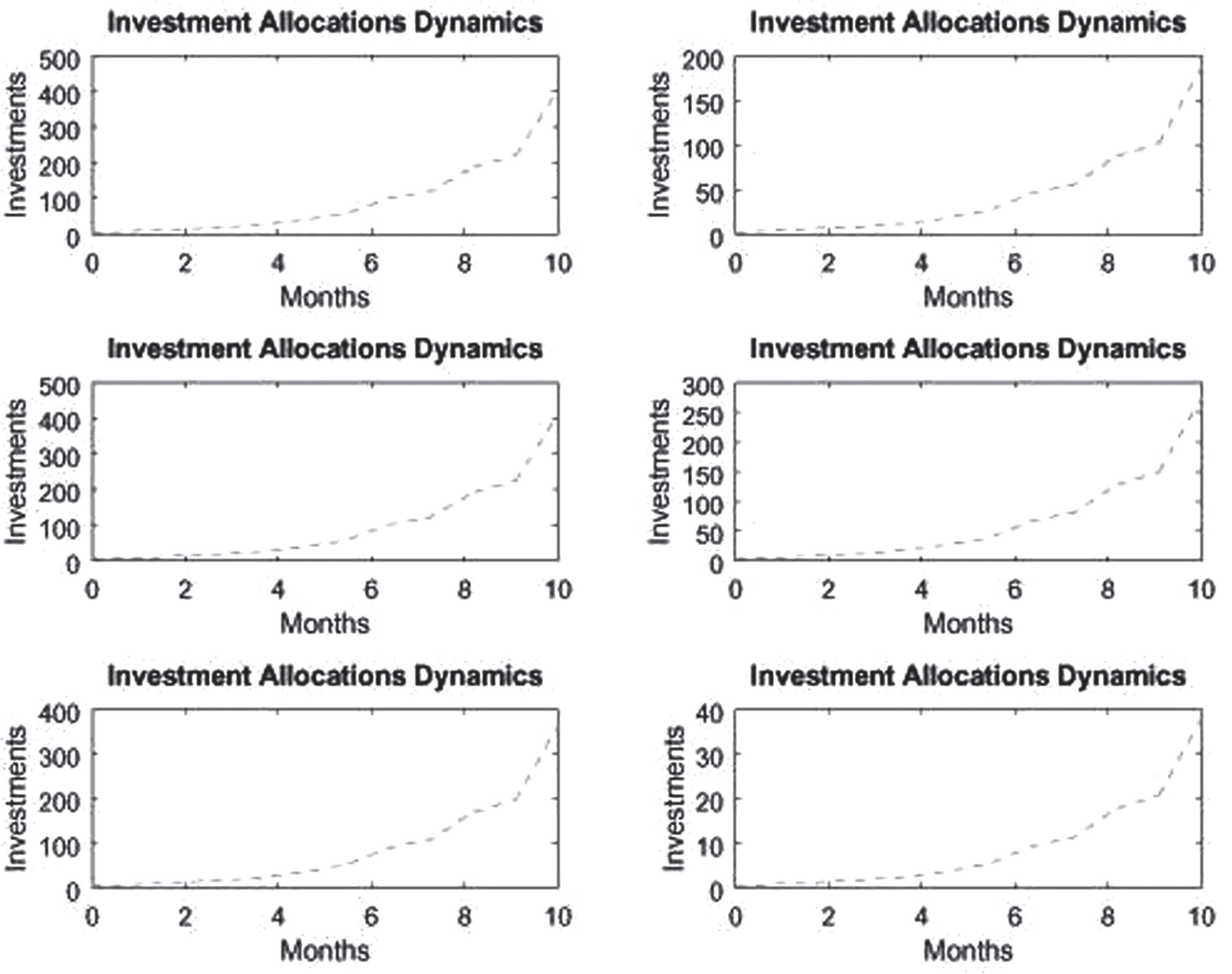
Plot of the Portfolio Stock Investment allocations.

Fig. 9

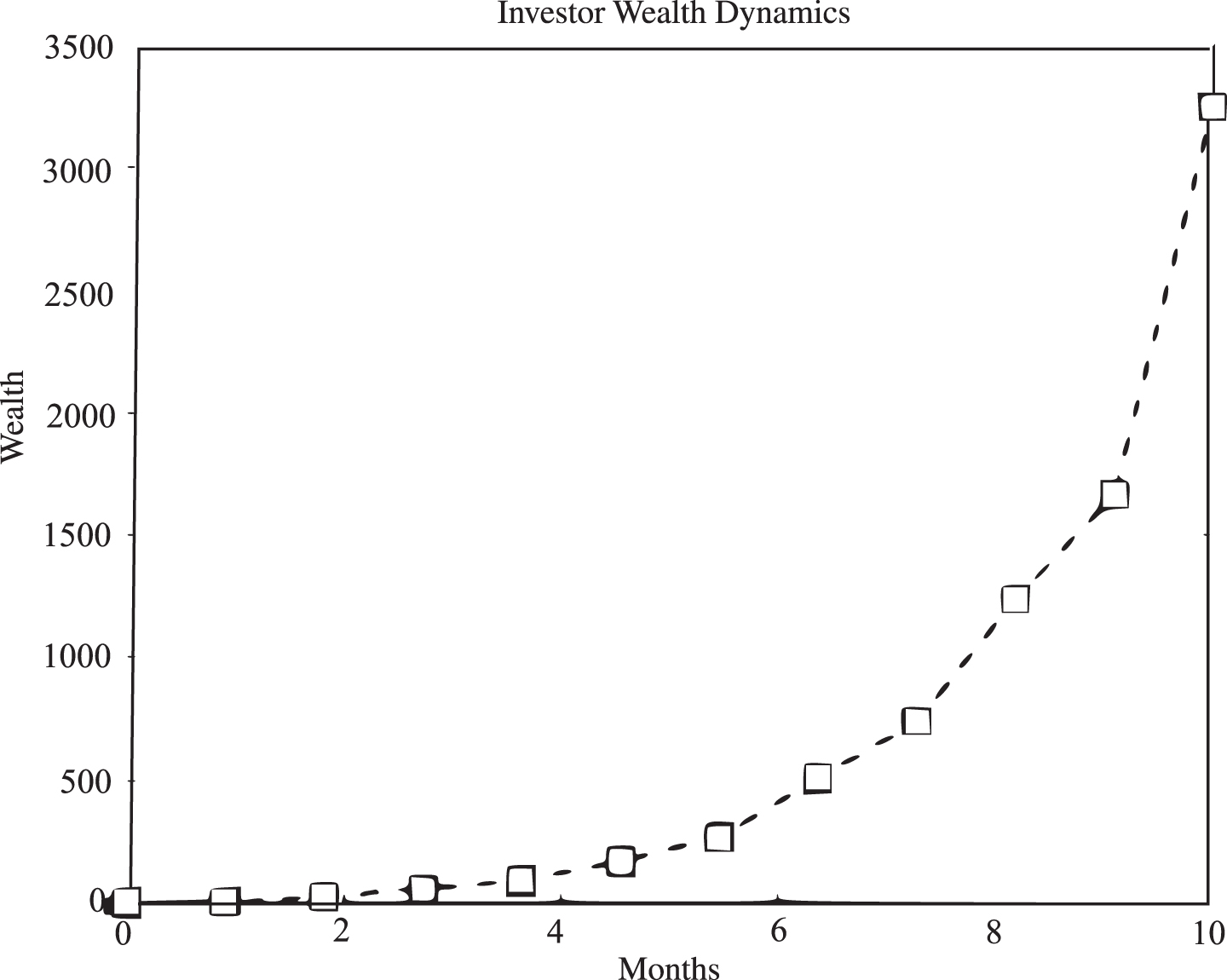
Plot of Wealth versus Time.

Fig. 10

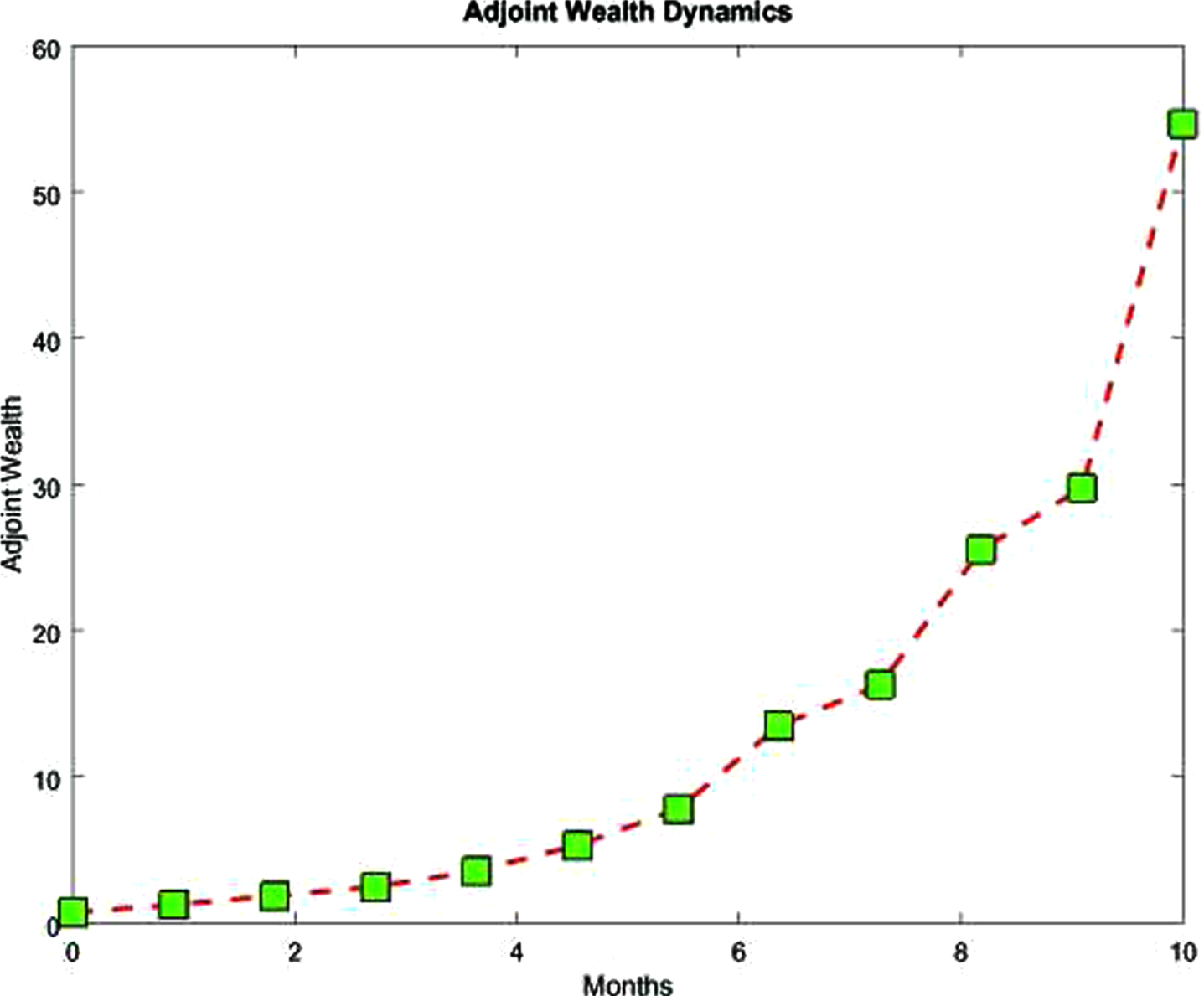
Plot of the costate process.

Fig. 11

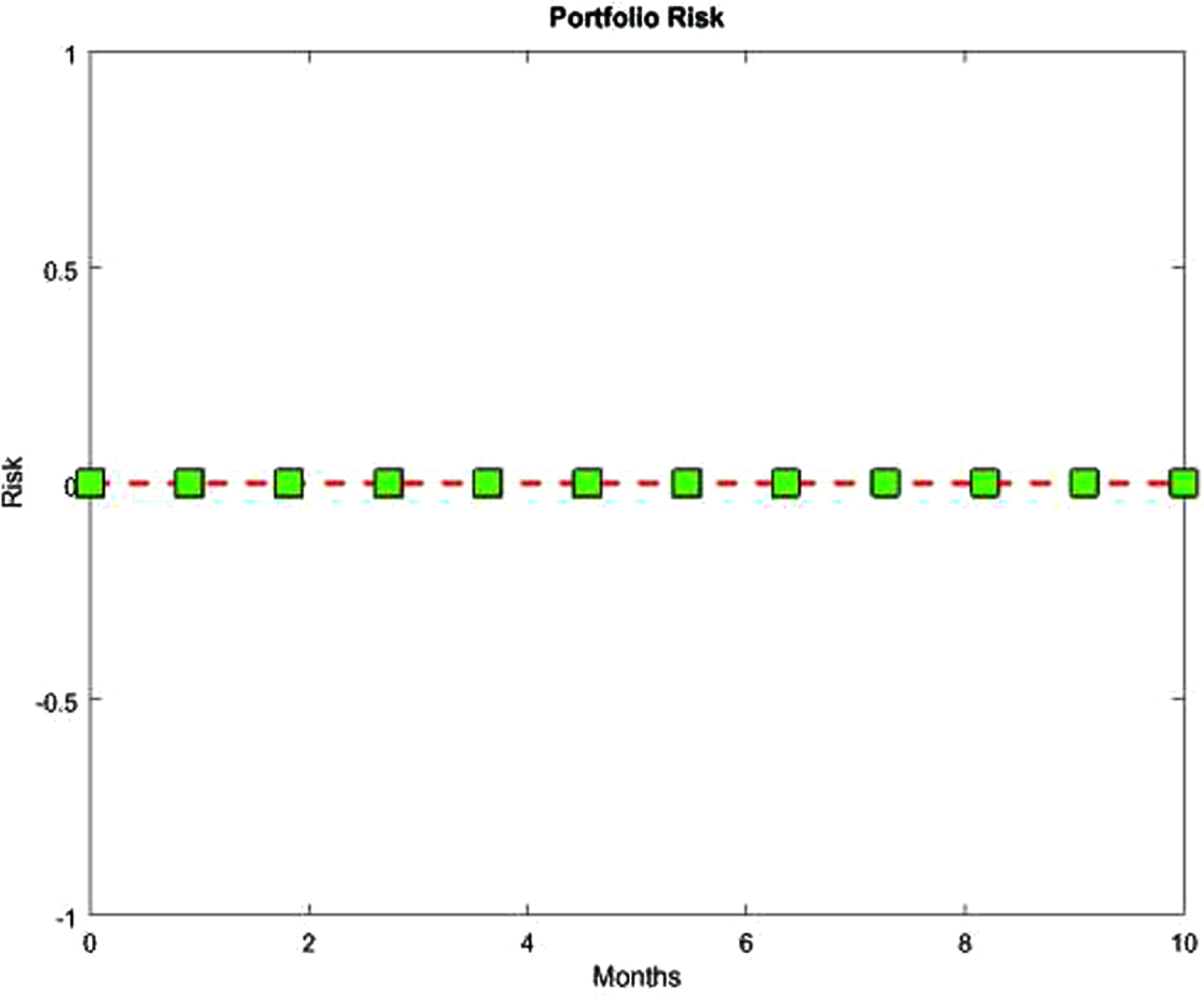
Plot of risk versus Time.

8 Portfolio profit maximization

The concern here is to compute optimal investment allocation processes such that the functional portfolio profit is maximized. Such a problem is defined as follows:

$\begin{matrix} Maximize 𝔼 [J (ω)] = 𝔼 {\int_{0}^{T} (μ Ω)^{2} dt} \\ = 𝔼 {\int_{0}^{T} (\sum_{i = 1}^{N} μ_{i} ω_{i})^{2} dt} \end{matrix}$ (52) subject to $\begin{matrix} dX (t) & = & {r (t) X (t) + \sum_{i = 1}^{m} [b_{i} (t) - r (t)] ω_{i}} dt \\ + \sum_{i = 1}^{m} \sum_{j = 1}^{m} σ_{ij} (t) ω_{i} (t) {dW}^{j} (t) \end{matrix}$ (53) $X (0) = X_{0} > 0$ (54) By dividing the left-hand side and the right-hand side of equation (2) by dt and by letting $Θ_{j} (t) = \frac{{dW}_{j}}{dt} (t)$ , then the above problem (52)-(2)can be approximately reformulated as follows:

$\begin{matrix} Maximize 𝔼 [J (ω)] = 𝔼 {\int_{0}^{T} (μ Ω)^{2} dt} \\ = 𝔼 {\int_{0}^{T} (\sum_{i = 1}^{N} μ_{i} ω_{i})^{2} dt} \end{matrix}$ (55) subject to $\begin{matrix} \frac{dX}{dt} (t) & = & {r (t) X (t) + \sum_{i = 1}^{m} [b_{i} (t) - r (t)] ω_{i} (t)} \\ + \sum_{j = 1}^{m} \sum_{i = 1}^{m} σ_{ij} (t) ω_{i} (t) Θ_{j} (t) \end{matrix}$ (56) $X (0) = X_{0} > 0$ (57) Equation (36) expresses the rate of change of total investor’s wealth. The Hamiltonian function is given by:

$\begin{matrix} H (t, X, ω_{1}, \dots, ω_{m}, λ) = L (t, X, ω_{1}, \dots, ω_{m}) \\ - λ f (t, X, ω_{1}, \dots, ω_{m}) . \end{matrix}$ (58) where

$L (t, X, ω_{1}, \dots, ω_{m}) = (\sum_{i = 1}^{N} μ_{i} ω_{i})^{2}$ (59)

$\begin{matrix} f (t, X, ω_{1}, \dots, ω_{m}) = r (t) X (t) + \sum_{i = 0}^{m} [b_{i} (t) - r (t)] ω_{i} \\ + \sum_{j = 0}^{m} \sum_{i = 0}^{m} σ_{ij} (t) ω_{i} (t) Θ_{j} (t) \end{matrix}$ (60)

To compute Ω = (ω₁ (t) , ..., ω_m (t)), first calculate the following expressions:

$\begin{matrix} \frac{\partial H}{\partial ω_{1}} & = & 2 μ_{1} \sum_{j = 1}^{m} μ_{j} ω_{j} - λ {(b_{1} - r) + \sum_{j = 1}^{m} σ_{1 j} Θ_{j}} \\ \frac{\partial H}{\partial ω_{2}} & = & 2 μ_{2} \sum_{j = 1}^{m} μ_{j} ω_{j} - λ {(b_{2} - r) + \sum_{j = 1}^{m} σ_{2 j} Θ_{j}} \\ ⋮ & ⋮ & ⋮ \\ \frac{\partial H}{\partial ω_{k}} & = & 2 μ_{k} \sum_{j = 1}^{m} μ_{j} ω_{j} - λ {(b_{k} - r) + \sum_{j = 1}^{m} σ_{kj} Θ_{j}} \\ ⋮ & ⋮ & ⋮ \\ \frac{\partial H}{\partial ω_{m - 1}} & = & 2 μ_{m - 1} \sum_{j = 1}^{m} μ_{j} ω_{j} - λ {(b_{m - 1} - r) + \sum_{j = 1}^{m} σ_{m - 1, j} Θ_{j}} \\ \frac{\partial H}{\partial ω_{m}} & = & 2 μ_{m} \sum_{j = 1}^{m} μ_{j} ω_{j} - λ {(b_{m} - r) + \sum_{j = 1}^{m} σ_{mj} Θ_{j}} \end{matrix}$ (61)

The first-order necessary conditions for optimality imply, ∀i = 1, ..., m let $\frac{\partial H}{\partial ω_{i}} = 0$ , lead to the following linear system of equations (where the unknowns are ω₁, ..., ω_m):

$\begin{matrix} 2 μ_{1} \sum_{j = 1}^{m} μ_{j} ω_{j} & = & λ {(b_{1} - r) + \sum_{j = 1}^{m} σ_{1 j} Θ_{j}} \\ 2 μ_{2} \sum_{j = 1}^{m} μ_{j} ω_{j} & = & λ {(b_{2} - r) + \sum_{j = 1}^{m} σ_{2 j} Θ_{j}} \\ ⋮ & ⋮ & ⋮ \\ 2 μ_{k} \sum_{j = 1}^{m} μ_{j} ω_{j} & = & λ {(b_{k} - r) + \sum_{j = 1}^{m} σ_{kj} Θ_{j}} \\ ⋮ & ⋮ & ⋮ \\ 2 μ_{m - 1} \sum_{j = 1}^{m} μ_{j} ω_{j} & = & λ {(b_{m - 1} - r) + \sum_{j = 1}^{m} σ_{m - 1, j} Θ_{j}} \\ 2 μ_{m} \sum_{j = 1}^{m} μ_{j} ω_{j} & = & λ {(b_{m} - r) + \sum_{j = 1}^{m} σ_{mj} Θ_{j}} \end{matrix}$ (62)

which can be rewritten in matrix form as:

$\begin{matrix} [\begin{matrix} μ_{11} & μ_{12} & \dots & μ_{1 m} \\ μ_{21} & μ_{22} & \dots & μ_{2 m} \\ ⋮ & ⋮ & ⋱ & ⋮ \\ μ_{k 1} & μ_{k 2} & \dots & μ_{km} \\ ⋮ & ⋮ & ⋱ & ⋮ \\ μ_{m 1} & μ_{m 2} & \dots & μ_{mm} \end{matrix}] [\begin{matrix} ω_{1} \\ ω_{2} \\ ⋮ \\ ω_{m} \end{matrix}] \\ = λ [\begin{matrix} b_{1} - r \\ b_{2} - r \\ ⋮ \\ b_{m} - r \end{matrix}] + [\begin{matrix} σ_{11} & σ_{12} & \dots & σ_{1 m} \\ σ_{21} & σ_{22} & \dots & σ_{2 m} \\ ⋮ & ⋮ & ⋱ & ⋮ \\ σ_{k 1} & σ_{k 2} & \dots & σ_{km} \\ ⋮ & ⋮ & ⋱ & ⋮ \\ σ_{m 1} & σ_{m 2} & \dots & μ_{mm} \end{matrix}] [\begin{matrix} Θ_{1} \\ Θ_{2} \\ ⋮ \\ Θ_{m} \end{matrix}] \end{matrix}$ (63) By letting $μ = [\begin{matrix} μ_{11} & μ_{12} & \dots & μ_{1 m} \\ μ_{21} & μ_{22} & \dots & μ_{2 m} \\ ⋮ & ⋮ & ⋱ & ⋮ \\ μ_{k 1} & μ_{k 2} & \dots & μ_{km} \\ ⋮ & ⋮ & ⋱ & ⋮ \\ μ_{m 1} & μ_{m 2} & \dots & μ_{mm} \end{matrix}]$ , $Ω = [\begin{matrix} ω_{1} \\ ω_{2} \\ ⋮ \\ ω_{m} \end{matrix}]$ , $b = [\begin{matrix} b_{1} \\ b_{2} \\ ⋮ \\ b_{m} \end{matrix}]$ and $Θ = [\begin{matrix} Θ_{1} \\ Θ_{2} \\ ⋮ \\ Θ_{m} \end{matrix}]$ , where μ_ij = μ_iμ_j with 1 ≤ i, j ≤ m, the system can be rewritten as:

$μ Ω = 0.5 λ (B - rI) + μ Θ$ (64) and then we find the value of Ω as

$Ω = 0.5 λ μ^{- 1} (B - rI) + Θ$ (65) where r ≥ 0, λ ∈ R, and I is a column vector of the same size as B and that contains one everywhere. Ω, Σ and Θ are specified as above. Given an initial condition of the system X (0) = X₀, consider the profit functional J given by (52), and consider the problem of computing a control ω (·) ∈ U for the wealth stochastic system such that J is maximized. By applying Pontryagin’s Maximum Principle Victor Emmanuel Becerra (2004), Dimitri P. Bertsekas (2000) and Jiongming Yong & Xun Yu Zhou (1999), the following is implied:

Since $Ω^{*} (t) = (ω_{1}^{*}, \dots, ω_{m}^{*}) \in U_{0}, t \in [0, T]$ is the optimal stochastic control process (the optimal investment allocation process strategy) for the above problem and X^* (t) , t ∈ [0, T] is the corresponding system response stochastic process, then there exists a function λ^* (t) , t ∈ [0, T], called the costate (or adjoint) process, such that the following equations are satisfied:

$\begin{matrix} Ω^{*} = (ω_{1}^{*}, \dots, ω_{m}^{*}) = λ^{*} μ^{- 1 *} (B - rI) + Θ^{*} \end{matrix}$ (66)

$\begin{matrix} \frac{{dX}^{*}}{dt} (t) = r (t) X^{*} (t) + \sum_{i = 0}^{m} [b_{i} (t) - r (t)] ω_{i}^{*} \\ + \sum_{j = 0}^{m} \sum_{i = 0}^{m} σ_{ij} (t) ω_{i}^{*} (t) Θ_{j} (t), X (0) = X_{0} \end{matrix}$ (67)

$\frac{d λ^{*}}{dt} (t) = r (t) λ^{*} (t), λ^{*} (0) = λ_{0}^{*}$ (68) The computational simulations for the profit maximization problem can be developed similarly as for the minimization problem and are left for the reader.

9 Conclusion

The aim of this paper was to compute optimal control processes to drive a controlled stochastic system from a given initial state to a final one such that the portfolio variance is minimized. To solve the problem, the following approach was used: Pontryagin’s Minimum Principle was applied to derive an Hamiltonian system of equations. Control processes were explicitly derived in terms of the state and costate processes. Finally, such control expressions were substituted into the state and the costate system of differential equations and a Matlab function was developed to code a fourth-order Runge-Kutta numerical method to solve, through a developed main function, the system formed by the state and costate equations (which were also coded into a Matlab function). From the above computational simulation comments, we can assess the relevance of approach. The above problem can also be solved by focusing on the objective functional and the Euler-Maruyama, Milstein, improved Euler or stochastic Runge-Kutta numerical method, as well as the initial state and define judiciously the control processes. Since the above problem is a stochastic linear quadratic problem, it can also be solved by using the stochastic Riccati equation as well as the stochastic Hamilton-Jacobi-Bellman principle or the control parameterization method.

Footnotes

Acknowledgment

The author thanks the university for the financial support.

References

Bjork,

, KHT, 2010. Stochastic Optimal Control with Finance Applications.

Chan,

, Sircar,

, 2016. Optimal trading with Predictable return and Stochastic Volatilty.

Chachuat,

B.C.

, 2007. Nonlinear and Dynamic Optimization, From Theory to Practice, Course Notes, Automatic Control Laboratory, Switzerland: EPFL.

2003, Formula Sheet for Optimal Control, Division of Optimization and System Theory, Royal Institute of Technology, Sweeden.

Kirk,

D.E.

, 1970. Optimal Control Theory, An Introduction, New-York: Prentice-Hall.

Kleywegt,

A.J.

, 2001. An Optimal Control Problem of dynamic Pricing. School of Industrial and System Engineering, Georgia institute of Technology. Atlanta, Georgia 30332-0205, USA.

Li,

, Zhou,

X.Y.

, 2006. Continuous-Time Mean-Variance Efficiency: The 80% Rule, The Annals of Applied Probability 16(4), 1751–1763.

Bielecki,

T.R.

, Jin,

, PLiska,

S.R.

, Zhou,

X.Y.

, 2005. Continuous Time Mean-Variance Portfolio Selection with bankruptcy prohibition. math. Finance 15, 213–244. MR2132190.

Li,

, NG,W.L. 2000. Optimal dynamic portfolio selection: Multi-period meanvariance formulation, Mathematics of Finance 10, 387–406. MR1800322.

10.

Powell,

W.B.

, 2018. A unified framework for Stochastic Optimization, European Journal of Operational Research.

11.

Mete Soner,

, Stochastic Optimal Control in Finance. Koc University. Istanbul, Turkey. msoner@ku.edu.tr.

12.

Lim,

A.E.B.

, 2004. Quadratic hedging and mean-variance portfolio selection with random parameters in an incomplete market, Math Oper Res 29, 132–161. MR2065719.

13.

Zhu,

, 2010. Uncertain Optimal Control with Application to a Portfolio selection Model. Cybernetics and Systems. September.

14.

Lim,

A.E.B.

, Zhou,

X.Y.

, 2002. Mean-variance portfolio selection with random parameters in an incomplete market, Math Oper Res 27, 101–120. MR1886222.

15.

Xia,

, 2005. Mean-variance portfolio choice: Quadratic Partial hedging, Math Finance 15, 533538, MR2147160.

16.

Zhou,

X.Y.

, Li,

, 2000. Continuous-Time Mean-Variance Portfolio Selection: A stochastic Linear Quadratic Framework. Applied Mathematics and Optimization 42, 19–33. Springer-Verlag New-York Inc.

17.

Becerra,

V.E.

, 2004. Solving Optimal Control Problems with State Constraints Using Nonlinear Programming and Simulation Tools, IEEE Transactions on Eduction 47(3).

18.

Markowits Harry,

, 1959. Portfolio selection: efficient diversification of investments, NewYork: Wiley.

19.

Carmona,

, Webster,

The Self-Financing Equation in High Frequency Markets.

20.

Duffie,

, 2001. Dynamic Asset Pricing Theory. Princeton, 3rd Edition.

21.

Bertsekas,

D.P.

, 2000. Dynamic Programming and Optimal Control, second edition, Athena Scientific, USA.

22.

Jiongming Yong Xun Yu Zhou., 1999. Stochastic Controls, Hamiltonian Systems and HJB Equations, Springer, New-York(USA).

23.

Jiang,

, Chen,

, Wang,

, Zhang,

J.E.

, Recovery of implied volatility: An optimal control approach.

24.

Krotov,

V.F.

, 1996. Global Methods In Optimal Control, Marcel Dekker, New-York, pp. 21–133.

25.

Becerra,

V.M.

, 2008. Optimal Control, UK: Scholarpedia.