Computation of financial risk using principal component analysis

Abstract

This article uses Principal Component Analysis to compute and extract the main factors for the financial risk of a portfolio, to determine the most dominating stock for each risk factor and for each portfolio and finally to compute the total risk of the portfolio. Firstly, each dataset is standardized and yields a new datasets. For each obtained dataset a covariance matrix is constructed from which the eigenvalues and eigenvectors are computed. The eigenvectors are linearly independent one to another and span a real vector space where the dimension is equal to the number of the original variables. They are also orthogonal and yield the principal risk components (pcs) also called principal risk axis, principal risk directions or main risk factors for the risk of the portfolios. They capture the maximum variance (risk) of the original dataset. Their number may even be reduced with minimum (negligible) loss of information and they constitute the new system of coordinates. Every principal component is a linear combination of the original variables (stock rate of returns). For each dataset, each financial transaction can be written as a linear combination of the eigenvectors. Since they are mutually orthogonal and linearly independent and that they capture the maximum variance of the original data, the risk of the portfolio is calculated by using the principal components, then they have been used to calculate the total risk of the portfolio which is a weighted sum of the variance explained by the principal components.

Keywords

Covariance matrix,eigenvalues and eigenvector financial transaction linear maps principal component analysis portfolio optimization risk analysis singular value decomposition stock price vector space

1 Introduction

Principal Component Analysis is an Unsupervised Machine Learning technique which is fundamentally a Mathematical Statistics and Data Analysis method. Very often Research in Engineering, in Economics and Finances, in Social, Political and Administrative sciences, in Psychology and Educational sciences, etc. involve hundreds of variables to represent the answer to a survey question. It is difficult even sometimes impossible to handle a big number of variables in a regression model, classification model and it poses a problem of dimensionality and redundancy preventing to analyse data easily and clearly and to visualize the results in a clear and understandable manner. Some of the variables are positively correlated in a such a way that they describe almost the same things so that using them together creates a problem of dimensionality and redundancy. Sometimes performing database queries for some selections in order to make relevant and reliable decisions becomes a tedious task. Principal Component Analysis is a technique of Mathematical Multivariate Statistics and Machine Learning to reduce dimensionality and remove redundancy while capturing maximum of data variation (minimizing loss of information). It enables to extract important information which can lead to the computation of relevant parameters in a simpler way. In this technique, the original variables can be combined in a particular manner so that they produce new variables where each of the new variables is a linear combination of the original variables. The new variables are linearly independent and called Principal Components. They generate a new axis coordinate system, a new reference system of coordinates. They indicate “latent” features that are not directly observable from the study subjects. The Principal Components are uncorrelated, linearly independent. The minimum number of principal components is one and the maximum number of Principal Components is the same as the number of the original variables. Depending on the researcher’s own judgement, the number of Principal Components can be reduced to a certain number while capturing information as much as possible.

In this article, a set of financial transactions of the original reference system of axis coordinate (where some of the underlying variables are linearly dependent vectors) will be orthogonally transformed into a set of financial transactions of the new reference system (where the underlying variables are linearly independent vectors), where each of these vectors is a linear combination of the original variables. Such vectors are called Principal Components, they produce Principal Axis, they are Principal variables, Principal Directions or principal factors. For each principal component, the order in which the coordinates (coefficients) in the matrix of eigenvectors are displayed is the same as the order in which the original variable values are listed at the starting table. Each principal component is a linear combination of the original variables. The components of the eigenvectors are the loadings, the weights of the principal components with respect to the original coordinate system variables. After having computed the eigenvalues and the associated eigenvectors of the covariance /correlation matrix of the rates of return, we have initially that the number of principal components is equal to the number of the original variables. It is important for the researcher to check rapidly after computation that the principal components are linearly independent. To check that the principal components are linearly independent it suffices to compute their covariance matrix and notice that it is a diagonal matrix with no zero element.

The theory of Principal Component Analysis can be intensively and popularly applied in Sciences, Humanities, Medicine (healthcare), Economics and Finances, Engineering, etc. and it has attracted a considerable research attention the last two decades. It can be used for crime signal detection, determination of the cities dominated by crime, disease signal detection, any feature detection, in crime intelligence, in crime detection, in security intelligence and analytics, in financial fraud detection, in principal disease sign detection, in face recognition, in earthquake signal detection, in tsunami detection, in remote sensing, in performance analysis, in disease diagnostic, in cancer detection, in drug effect estimation, in financial risk estimation, in data Filtering, data denoising, in data Compression for optimal storing and transfer, in noise detection and management, etc. It is used in Geology and Geo-Physics to solve the problem of Earth Quake Detection, Petrol and Mining Exploration, etc. It is used in Cellular and Molecular Biology and also in Medecine to analyze and solve heath problems related to Cardiology, Epidemiology, Cancer detection, the effect of different types of drugs in the human body, etc., in Biology to compare species, in Finances to detect inflation or growth, to detect fraud, to classify financial assets, to select a portfolio of financial instruments contributing the most to the life of the portfolio while minimizing the ones whose actions are negligible. There exist some works carried out on Principal Component Analysis. In Perlibakas (2004) the author proposed PCA or Karhunen-Loeve transform (KLT)-based face recognition method. It was studied by computer scientists and Psychologists and used as a baseline method for comparison of face recognition methods and implemented in commercial applications. Using PCA we find a subset of principal directions (principal components) in a set of training faces. Then we project faces into this principal components space and get feature vectors. Perlibakas (2004) compared 14 distance measures and their modifications between feature vectors with respect to the recognition performance of the pca-based face recognition method and propose modified sum square error (SSE)-based distance. Zong, Marcel and Galvasas (2014) proposed a different reconstruction method to perform compressed sensing by using pca. Such the experiment, demonstrate that this method can reduce analysis. They showed through the experiments, demonstrate that this method can reduce analysis. They showed through the experiments that this method can reduce a liasing artefacts and achieve a high peak signal to noise. Murali (2015) used a simple and efficient method to extract feature vector from images and to reduce the dimension of data. PCA is used for face recognition technique for feature...Khan and Farooq (2011) uses pca and LDA to design a system. It presents the realization of such technologies which demands reliable and error-free high dimensional patterns are not permitted due to eigen-decomposition in high dimensional image space ad degeneration of scattering matrices. Wang, Quanxue, Xinbo and Nie (2017) proposed a novel formulation of PCA, namely angle PCA. Such a formulation was developed to handle the fact that the development of many l₁-norm based pca methods do not explicitly consider the reconstruction error and variance of projected data.

In this paper, the theory of Principal Component Analysis is applied to compute and extract the main financial risk factors for each of the portfolios, to determine (for each risk factor) the most dominating stock, to determine the total risk (for each portfolio) and to determine (for each portfolio risk) the stock contributing the most. Risk Estimation is an important issue for financial market operators. There exist many ways of estimating portfolio financial risk. In this paper financial risk is going to be analysed and estimated by using Principal Component Analysis. Such a risk is going to be estimated from a given dataset which is constituted by historical data of stock rates of return. This paper is related to Quantitative Finances, Algorithmic Finance, Data Science and Optimization. The aim is to use an unsupervised machine learning technique called PCA to compute the main financial risk factors for each portfolio and then the portfolio risks. It proposes a way of computing and measuring the financial risk of a stock portfolio.

It is generally known that the PCA technique allows the user to determine the axis which capture the maximum variance of a given dataset. Since financial risk is strongly related to variation of the data, this article aims to see if the PCA can also constitute a way of calculating the risk for a portfolio. Firstly, each multivariate time series for rate of return for stocks was normalized to prepare all the time series to have the same scale to ease the interpretation of the results. Secondly, for each multivariate time series, a covariance matrix was designed and diagonalized. Thirdly, the eigenvalues and the associated eigenvectors were computed. From the eigenvectors, the principal components scores are computed. Such principal components constitute the main factors of risk. From each factor, the dominating stock is extracted. From the eigenvalues, the total risk of the portfolio was computed.

It is stated that to each multivariate time series is associated a portfolio. For each of the portfolios the substantive contributions of this article are the main factors of risk, the proportions of risk explained by the principal components, the dominating stock for each factor, the total portfolio risk and the dominating stock for each portfolio. The main factors of risk are obtained from the eigenvectors of the covariance matrices. The proportions of variances (risks) explained by the principal components are obtained from the eigenvalues of the covariance matrices. Each of the covariance matrices is obtained from a standardized multivariate time series.

The research associated to this paper provides rigorous ways for collecting, cleaning, processing and analyzing financial data, for computing, predicting and managing the associated risk factors which are major issues for the financial market operators and which are very interesting to financial engineers, financial economists, financial mathematicians and financial computer scientists. Such ways can also be adapted in other areas. Since the technique used shows how much variation is captured by the obtain principal components, the PCA technique can also be used to solve Capital Budgeting Design, Financial Portfolio Construction, Portfolio Immunization, Financial Data Compression, Financial Noise Management, Financial Noise Removal, Drug effect on human body, Financial Data Encryption in Cryptography, Image Analysis for Heathcare, Financial Signal Processing and Analysis, Financial Anomaly Detection. It can also be used to predict the feasibility of a Telecommunication system configuration, to predict the feasibility of a Power network system configuration, to predict the performance of a computer network system, to assess the feasibility of a short term or a long term project.

The contributions of this paper are the computation of the main financial risk factors, the determination of the dominating stock for each risk factor, the determination of the dominating stock for the whole portfolio and the computation of the portfolio risk based on the principal components algebraic and statistical properties.

The paper is subdivided into the following sections: Section 2 states precisely the problem. Section 3 describes some linear algebra and algebraic geometry notions associated to the notion of principal component analysis. Section 4 presents briefly the approach to solve the problem. Section 5 solves the problem by applying PCA on each of the three multivariate time series and discusses on the results. Section 5 concludes the article.

2 Problem Formulation

Given three historical datasets D₁,D₂andD₃. They are associated respectively to the multivariate time series R₁,R₂andR₃where each of them presents as a matrix with M periods of time representing the rows and Nfinancial variables representing the columns. For each multivariate time series, the variables are the rates of return for stocks and constitute respectively the three portfolios π₁,π₂andπ₃. By normalizing (standardizing) each of the above multivariate timeseries and by computing the covariance matrix of each of them we obtain the covariance matrices respectively denoted as Σ₁,Σ₂andΣ₃. Notice that R₁, R₂andR₃are obtained respectively from D₁,D₂andD₃by excluding the first column listing the period of time labels and the first row listing the stock labels. The dataset D₁,D₂andD₃correspond to the portfolios π₁,π₂andπ₃. This paper addresses for each of the portfolios the following problems:

Computation and extraction of the main factors of financial risk.

Determination of the dominating stock for each of the computed factors.

Computation of the resultant of the main factors.

Determination of the dominating stock for each resultant.

Computation of the total risk.

3 Linear Algebra, Algebraic Geometry and Multivariate Statistics Background

The questions of this paper take us to the application of some notions of Linear Algebra and Multivariate Statistics. The original reference system of coordinates as well as the new reference system of coordinates spanned a real vector space where the dimension is equal to the number of the original variables. So, the theory of vector space is relevant. The orthogonal transformation of the original reference system of coordinates into the new reference system of coordinates is performed through a linear map. Each eigenvalue of the covariance matrix of the multivariate time series is associated to an eigen subspace which is also a vector space from which a basis of eigenvector(s) can be extracted. The eigenvectors all together form a linearly independent family of vectors. Such vectors lead to the computation of the principal components which shows how relevant is the theory of linear dependence in the principal component analysis as an unsupervised machine learning technique. The principal component analysis as an unsupervised machine learning technique in data analysis is based on the fact that the number of variables is big and that some of the variables in the multivariate time series under study are correlated so that they create redundancy and confusion. One of the aim of the computation of principal components is to remove redundancies in the given multivariate time series by performing orthogonal projection of each of the given financial transactions from the original vector space into the new vector space, the vector space spanned by the set of principal components and by keeping the most relevant principal components, the ones capturing the maximum of variation of the data. This technique consists of linearly grouping the original variables and generate others which must be uncorrelated and thus linearly independent. In the orthogonal projection, the rotation matrix (the matrix storing the eigenvectors as columns) is multiplied by each of the financial transactions to generate new dataset where the underlying variables are linearly independent and from which we can select the most relevant, the ones capturing the maximum of variability of the information. If the new variables undergo the same operations as the original ones the covariance matrix will give a diagonal matrix. When the dataset is very big, one may perform matrix factorization to decompose the underlying matrix and process data in a very judicious way. The computation of eigenvalues and eigenvectors is performed through the solving linear system of algebraic equations. The question aiming to compute the principal components involves the applications of function spaces, projection of a function in a function space without excluding the notion of variance of a random variable which corresponds to the notion of a norm of a vector, norm of a random vector, correlation and covariance between random variables which correspond to the notion of projection of a vector in the direction of another vector also similar to scalar (dot) product between two vectors. The notion of risk(variance) and factors corresponds to that of eigenvalue and eigenvectors.

In tackling the problem using PCA, one must assume that some of the variables which are the rate of return stock time series are linearly correlated. The aim may also be to reduce the number of variables / columns of the associated matrix storing them so that data can be displayed and described in a understandable and efficient manner. We need also to investigate on the variability of the multivariate time series under study and see how each of the stocks contributes to this variability. Indeed, to normalize or standardize a multivariate time series, for each stock time series, the mean must be subtracted from each element of that time series and divided by the standard deviation. Such an operation is performed to normalise the data and change them into the same scale to avoid ambiguous interpretation of results. From the normalized data, compute the covariance / correlation matrix Σ. The covariance matrix Σ, as a symmetric matrix, is subject to a certain number of properties which involve and constrain the range for the eigenvaluesλ₁, . . . , λ_Nand eigenvectors s v₁, . . . , v_N.

Since the covariance / correlation matrix is symmetric positive definite, then all its eigenvalues are real and positive. It is obviously known that the eigenvalues are the roots of a characteristic polynomial and that the characteristic polynomial of a matrix is obtained by computing the determinant of the matrix obtained by subtracting a diagonal matrix where having the same diagonal on the diagonal from the original matrix.

From the covariance / correlation matrix denoted Σ, construct the characteristic polynomial and the associated characteristic equation to compute the eigenvalues and the associated eigenvectors. Notice that every eigenvector is extracted from the basis of the associated eigensubspace. The transformation is performed such that the first principal component has the highest possible variance and each succeeding principal component has the largest variance and is orthogonal to the preceding.

The first eigenvector (first principal component) is the eigenvector associated with the largest eigenvalue. The second eigenvector is the eigenvector associated with the second largest eigenvalue and is orthogonal to the first principal component. Every following eigenvector is associated to a following eigenvalue and is orthogonal to each of the previous eigenvector. Once all the results of the principal component analysis are obtained, the interpretations and recommendations are based on the size and sign of eigenvalues, the components of the eigenvectors, the proportion of variance that each component explains.

4 Solution approach to the problem

Three datasets D₁,D₂andD₃are considered. To tackle the problem in a precise way, ∀k = 1, 2, 3do the following: To each dataset D_kis associated a multivariate time series R_k = R_ij. To each multivariate time seriesR_k = R_ijis associated a portfolio π_k. ∀k = 1, 2, 3 R_k = R_ijcan then be displayed as a matrix storing the rates of return during M periods of time and which concern N financial stocks. Thus the matrix R_k = R_ijhas M rows and N columns. We have that ∀i = 1, . . . , M j = 1, . . . , NR_k = R_ijis the rate of return at period i and for the stock number j, the rate of return in month i and for stock number j.

Indeed, notice that for each of the portfolios we are given N stocks and each stock is concerned with a time series of size M. By picturing, displaying and storing vertically all the time series in a matrix we then have the above-mentioned matrix R_k where the rows are the observation periods also called transaction periods and the columns are the variables concerning the stocks. each variable is a rate of return for a certain stock. In this paper every period of time is a month. 30 months are considered for each of the three multivariate time series, and each multivariate time series is associated to a portfolio. In total, for each portfolio we have 30 financial transactions and each transaction involves seven stocks.

Based on the matrix R_k, computer programs are written in Matlab and Scilab to compute the covariance matrices, from each covariance matrix the eigenvalues and the associated eigenvectors are computed. Each eigenvalue indicates the proportion of variance explained by its corresponding principal component. From each of the eigenvector components and the original variables we obtain the principal component scores. For each multivariate time series / portfolio the principal components we determine the main factors for the risk. From the expression of each principal component as a linear combination of the original variables, the original variables (rates of return) with the maximum absolute value coefficient is the most dominating. After running the computer programs, we obtain the eigenvalues and for each eigenvalue the associated eigensubspace was obtained from which a basis of the eigenvector was extracted. The eigenvectors give the coefficients of each of the principal components with respect to the original variables. From the eigenvectors, the principal component scores are determined. the Hotelling as well as the means of the original variables are computed.

5 Application of the PCA to the given dataset (multivariate time series)

5.1 Application of the PCA to the first dataset

5.1.1 Introduction

The first given dataset D₁ is constituted by the stock time series. D₁ is the collection of the time series of stocks. In this case we have 7 stocks. Statistically speaking, D₁ is a multivariate time series and store it into Table 1. The rows of D₁ in Table 1 are the stock observations (the instantaneous stock rate of return vectors) and the columns are the data variables called stocks. By letting D₁ = [X₁, X₂, X₃, X₄, X₅, X₆, X₇], we have that Xi = Stock_i ∀i = 1, . . . , 7. The columns of Table 1 are represented by the variables X₁, X₂, X₃, X₄, X₅, X₆ and X₇. Each of them is a stock rate of return time series of length 30. By letting D₁ = (R_ij) we have that R_ij is the rate of return at period i of stock j. Let Σ be the covariance matrix of D₁. It means that we have Σ = (cov (X_i, X_j)) , i, j = 1, . . . , 7. The eigenvectors of Σ are linearly independent and spanned a vector space of dimension equal to the number of the original variables which is 7. Their components represent the coefficients of the principal components (new variables) with respect to the original variables (the stocks). They are the columns and are stored in matrix cfA. The matrix cfA can be rewritten and stored explicitly in Table 2. We have that X_i, i = 1, …, 7are the original variables and the pc_i, i = 1, …, 7are the new variables called principal components, principal axis, principal factors.

Table 1
Stock Returns during 30 months

Months Stock1 Stock2 Stock3 Stock4 Stock5 Stock6 Stock7

January 0.5500 0.0600 0.5900 0.5100 0.0800 0.1600 0.1000

February 0.4000 0.1100 0.3900 0.4600 0.3400 0.3800 0.1800

March 0.3800 0.2200 0.3300 0.0800 0.1000 0.5700 0.1200

April4 0.2200 0.2000 0.4000 0.2600 0.3700 0.2700 0.1000

May 0.3000 0.0100 0.5400 0.3900 0.0100 0.0800 0.3900

June 0.4700 0.3600 0.3500 0.3000 0.5000 0.2900 0.5900

July 0.5800 0.0700 0.1400 0.0400 0.5600 0.2000 0.6200

August 0.4700 0.1000 0.3000 0.1500 0.6000 0.2700 0.1500

September 0.0200 0.4200 0.2800 0.5500 0.6500 0.5500 0.3200

October 0.4400 0.5600 0.6300 0.0200 0.3300 0.2700 0.2500

November 0.2900 0.6400 0.4100 0.5700 0.1800 0.2600 0.3500

December 0.2900 0.3800 0.4600 0.0600 0.0700 0.2400 0.1800

January 0.0800 0.6500 0.4700 0.4400 0.3400 0.1000 0.0500

February 0.5300 0.3600 0.2300 0.3300 0.3900 0.1700 0.2900

March 0.2200 0.3400 0.3400 0.1500 0.5000 0.0600 0.1200

April 0.1700 0.2200 0.3700 0.3800 0.0600 0.2800 0.0200

May 0.2300 0.2800 0.1100 0.0800 0.4400 0.1700 0.6300

June 0.2500 0.3200 0.3700 0.4400 0.3400 0.2000 0.2800

July 0.3600 0.0500 0.4600 0.3900 0.1200 0.2800 0.6300

August 0.3700 0.5800 0.2800 0.0400 0.6200 0.0800 0.5000

September 0.2600 0.0500 0.5500 0.0400 0.3900 0.3300 0.0100

October 0.2600 0.2900 0.4800 0.1000 0.2900 0.4600 0.4500

November 0.3400 0.5400 0.2400 0.0200 0.6200 0.1600 0.4600

December 0.4300 0.2600 0.3000 0.2900 0.4300 0.5200 0.4200

January 0.6200 0.4000 0.2600 0.5500 0.3000 0.0500 0.3600

February 0.4700 0.5400 0.5100 0.4100 0.5500 0.2600 0.1500

March 0.2700 0.5800 0.4800 0.3400 0.3500 0.0100 0.5100

April 0.5500 0.6100 0.2800 0.5700 0.3700 0.1500 0.1500

May 0.0900 0.1300 0.4600 0.0700 0.4500 0.0100 0.2500

June 0.0400 0.1700 0.6200 0.6000 0.2400 0.1300 0.5800

Months	Stock1	Stock2	Stock3	Stock4	Stock5	Stock6	Stock7
January	0.5500	0.0600	0.5900	0.5100	0.0800	0.1600	0.1000
February	0.4000	0.1100	0.3900	0.4600	0.3400	0.3800	0.1800
March	0.3800	0.2200	0.3300	0.0800	0.1000	0.5700	0.1200
April4	0.2200	0.2000	0.4000	0.2600	0.3700	0.2700	0.1000
May	0.3000	0.0100	0.5400	0.3900	0.0100	0.0800	0.3900
June	0.4700	0.3600	0.3500	0.3000	0.5000	0.2900	0.5900
July	0.5800	0.0700	0.1400	0.0400	0.5600	0.2000	0.6200
August	0.4700	0.1000	0.3000	0.1500	0.6000	0.2700	0.1500
September	0.0200	0.4200	0.2800	0.5500	0.6500	0.5500	0.3200
October	0.4400	0.5600	0.6300	0.0200	0.3300	0.2700	0.2500
November	0.2900	0.6400	0.4100	0.5700	0.1800	0.2600	0.3500
December	0.2900	0.3800	0.4600	0.0600	0.0700	0.2400	0.1800
January	0.0800	0.6500	0.4700	0.4400	0.3400	0.1000	0.0500
February	0.5300	0.3600	0.2300	0.3300	0.3900	0.1700	0.2900
March	0.2200	0.3400	0.3400	0.1500	0.5000	0.0600	0.1200
April	0.1700	0.2200	0.3700	0.3800	0.0600	0.2800	0.0200
May	0.2300	0.2800	0.1100	0.0800	0.4400	0.1700	0.6300
June	0.2500	0.3200	0.3700	0.4400	0.3400	0.2000	0.2800
July	0.3600	0.0500	0.4600	0.3900	0.1200	0.2800	0.6300
August	0.3700	0.5800	0.2800	0.0400	0.6200	0.0800	0.5000
September	0.2600	0.0500	0.5500	0.0400	0.3900	0.3300	0.0100
October	0.2600	0.2900	0.4800	0.1000	0.2900	0.4600	0.4500
November	0.3400	0.5400	0.2400	0.0200	0.6200	0.1600	0.4600
December	0.4300	0.2600	0.3000	0.2900	0.4300	0.5200	0.4200
January	0.6200	0.4000	0.2600	0.5500	0.3000	0.0500	0.3600
February	0.4700	0.5400	0.5100	0.4100	0.5500	0.2600	0.1500
March	0.2700	0.5800	0.4800	0.3400	0.3500	0.0100	0.5100
April	0.5500	0.6100	0.2800	0.5700	0.3700	0.1500	0.1500
May	0.0900	0.1300	0.4600	0.0700	0.4500	0.0100	0.2500
June	0.0400	0.1700	0.6200	0.6000	0.2400	0.1300	0.5800

Table 2

Eigenvectors

variables	pc₁	pc₂	pc₃	pc₄	pc₅	pc₆	pc₇
X₁	0.1319	-0.0525	0.1447	0.8576	-0.3887	0.1051	0.2476
X₂	0.3359	0.7649	-0.2552	-0.0741	-0.1521	0.4544	-0.0425
X₃	-0.3536	0.0380	-0.0630	-0.2865	-0.2019	0.1275	0.8547
X₄	-0.4166	0.5970	0.4429	0.2211	0.3798	-0.2814	0.0396
X₅	0.6202	0.0603	-0.2023	0.0530	0.3764	-0.4997	0.4202
X₆	-0.0724	-0.2043	-0.1421	0.2331	0.7062	0.6037	0.1236
X₇	0.4258	-0.0941	0.8079	-0.2664	0.0161	0.2700	0.1141

5.1.2 Interpretation of the eigenvector coefficients

Table 2 below displays the eigenvectors of the covariance matrix of the dataset defined by Table 1. It displays every eigenvector coefficients with respect to the original variables from whichthe results displayed in Table 2, one can notice the following:

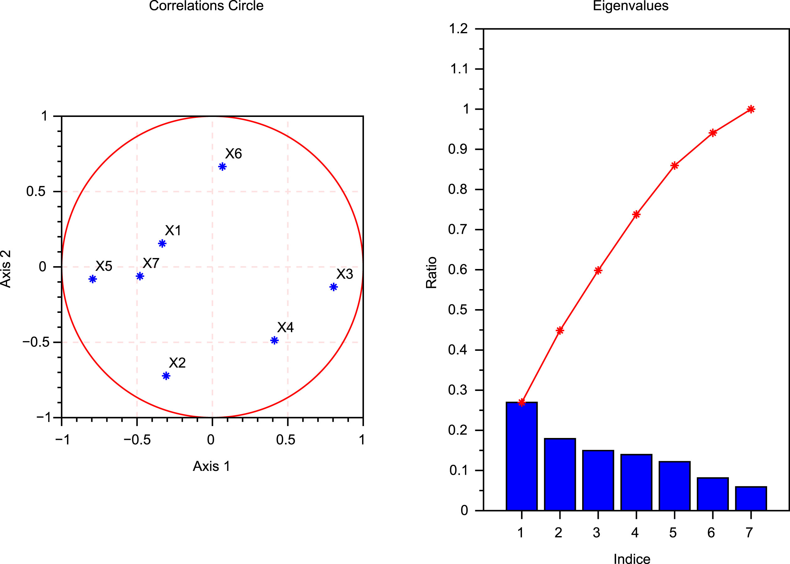
0.6202 is the first column’s maximum value in absolute value. It is the coefficient of the first principal component with respect to variable 5 which is the stock number 5. Thus, the first principal component has the largest positive association with the stock number 5. In other words, stock number 5 is the most dominating variable to the construction of the first factor.

0.7649is the second column’s maximum value in absolute value. It is the coefficient of the second principal component with respect to variable 2 which is the stock number 2. Thus, the second principal component has the largest positive association with the stock number 2. In other words, stock number 2 is the most dominating variable for the construction of the second factor.

0.8079is the third column’s maximum value in absolute value. It is the coefficient of the third principal component with respect to variable 7 which is the stock number 7. Thus, the third principal component has the largest positive association with the stock number 7. In other words, stock number 7 is the most dominating variable for the construction of the third factor.

0.8576is the fourth column’s maximum value in absolute value. It is the coefficient of the fourth principal component with respect to variable 1 which is the stock number 1. Thus, the fourth principal component has the largest positive association with the stock number 1. In other words, stock number 1 is the most dominating variable in the construction of the fourth factor.

0.7062is the fifth column maximum’s value in absolute value. It is the coefficient of the fifth principal component with respect to variable 6 which is the stock number 6. The fifth principal component has the largest positive association with the stock number 6. In other words, stock number 6 is the most dominating variable in the construction of the the fifth factor.

0.6037is the sixth column maximum’s value in absolute value. It is the coefficient of the sixth principal component with respect to variable 6 which is the stock number 6. The sixth principal component has the largest positive association with the stock number 6. In other words, stock number 6 is the most dominating variable in the construction of the sixth factor.

0.8547is the seventh column maximum value in absolute value. It is the coefficient of the seventh principal component with respect to variable 3 which is the stock number 3. The seventh principal component has the largest positive association with the stock number 3. In other words, stock number 3 is the most dominating variable in the construction of the seventh factor.

5.1.3 Derivation of the principal components

It is known that each principal component pcA_i, as a new variable, is a linear combination of the original variables X_i. The linear combination coefficients are obtained from the orthogonal matrix whose columns are the eigenvectors. Define cfA₁, cfA₂, cfA₃, cfA₄, cfA₅, cfA₆ and cfA₇ to be the columns of cfA.

Then we may write cfA = [cfA₁, cfA₂, cfA₃, cfA₄, cfA₅, cfA₆, cfA₇] which is the orthogonal matrix of the problem. cfA_i is the column number i of matrix cfA.

Define pcA_i i = 1, . . . , 7 to be the columns of the matrix pcA containing the detailed principal components also called principal component analysis scores. Every pcA_i is a column vector of length equal to that of every original variable. We obtain the principal component analysis scores by using the following rules: ${pcA}_{1} = \sum_{i = 1}^{7} cfA (i, 1) * X_{i};$ (1) ${pcA}_{2} = \sum_{i = 1}^{7} cfA (i, 2) * X_{i};$ (2) ${pcA}_{3} = \sum_{i = 1}^{7} cfA (i, 3) * X_{i};$ (3) ${pcA}_{4} = \sum_{i = 1}^{7} cfA (i, 4) * X_{i};$ (4) ${pcA}_{5} = \sum_{i = 1}^{7} cfA (i, 5) * X_{i};$ (5) ${pcA}_{6} = \sum_{i = 1}^{7} cfA (i, 6) * X_{i};$ (6) ${pcA}_{7} = \sum_{i = 1}^{7} cfA (i, 7) * X_{i} .$ (7) where cfA (i, j)is the coefficient or component number i of the principal component number j. It is the component of pcA_j with respect to the original variable X_i ∀ i, j = 1, . . . , 7.

The principal components pcA_i, i = 1, . . . , 7of the given dataset, are columns of pcA.

Each principal component is a linear combination of the original variables. The principal component scores are stored in the matrix pcA. One can notice that the principal components are linearly independent and orthogonal. each row of pcA is obtained by performing orthogonal projection of the corresponding row of D₁.

$cfA = [\begin{matrix} 0.1319 & - 0.0525 & 0.1447 & 0.8576 & - 0.3887 & 0.1051 & 0.2476 \\ 0.3359 & 0.7649 & - 0.2552 & - 0.0741 & - 0.1521 & 0.4544 & - 0.0425 \\ - 0.3536 & 0.0380 & - 0.0630 & - 0.2865 & - 0.2019 & 0.1275 & 0.8547 \\ - 0.4166 & 0.5970 & 0.4429 & 0.2211 & 0.3798 & - 0.2814 & 0.0396 \\ 0.6202 & 0.0603 & - 0.2023 & 0.0530 & 0.3764 & - 0.4997 & 0.4202 \\ - 0.0724 & - 0.2043 & - 0.1421 & 0.2331 & 0.7062 & 0.6037 & 0.1236 \\ 0.4258 & - 0.0941 & 0.8079 & - 0.2664 & 0.0161 & 0.2700 & 0.1141 \end{matrix}]$

$pcA = [\begin{matrix} - 0.4738 & - 0.0496 & 0.0810 & 0.2213 & - 0.1592 & - 0.0934 & 0.0994 \\ - 0.2059 & - 0.0778 & 0.0178 & 0.1790 & 0.1674 & - 0.0734 & 0.0329 \\ - 0.1802 & - 0.2694 & - 0.2046 & 0.1344 & 0.0692 & 0.2922 & - 0.1273 \\ - 0.1271 & - 0.0867 & - 0.1755 & - 0.0319 & 0.0781 & - 0.0968 & - 0.0250 \\ - 0.3701 & - 0.1635 & 0.2674 & - 0.1012 & - 0.1681 & - 0.0500 & - 0.0140 \\ 0.2485 & 0.0022 & 0.2075 & 0.0749 & 0.0528 & 0.0639 & 0.1019 \\ 0.4046 & - 0.3694 & 0.2204 & 0.1676 & - 0.0427 & - 0.0861 & - 0.0308 \\ 0.1174 & - 0.2366 & - 0.1623 & 0.1931 & 0.0619 & - 0.1992 & 0.0537 \\ 0.0891 & 0.1996 & - 0.0433 & - 0.0997 & 0.5634 & - 0.0263 & 0.0024 \\ 0.0806 & 0.0261 & - 0.2270 & - 0.0309 & - 0.2125 & 0.2472 & 0.2015 \\ - 0.1134 & 0.3987 & 0.1008 & - 0.0178 & 0.0251 & 0.1809 & - 0.0581 \\ - 0.1451 & - 0.0893 & - 0.1741 & - 0.0908 & - 0.1974 & 0.2097 & - 0.0926 \\ - 0.1217 & 0.4126 & - 0.2455 & - 0.1934 & - 0.0139 & - 0.0499 & - 0.0512 \\ 0.0990 & 0.0585 & 0.0339 & 0.2134 & - 0.0659 & - 0.0520 & - 0.0799 \\ 0.0913 & 0.0013 & - 0.2365 & - 0.0968 & - 0.0719 & - 0.1962 & - 0.0557 \\ - 0.3934 & - 0.0115 & - 0.1361 & - 0.0339 & 0.0352 & 0.0088 & - 0.1973 \\ 0.3549 & - 0.1697 & 0.1723 & - 0.1467 & 0.0165 & 0.0020 & - 0.2034 \\ - 0.0841 & 0.1054 & 0.0413 & - 0.0325 & 0.0647 & - 0.0723 & - 0.0419 \\ - 0.1645 & - 0.1959 & 0.4142 & - 0.0412 & 0.0052 & 0.0949 & 0.0291 \\ 0.4935 & 0.0765 & - 0.0411 & - 0.0832 & - 0.1310 & 0.0066 & 0.0119 \\ - 0.1639 & - 0.3318 & - 0.3236 & - 0.0391 & 0.0199 & - 0.0778 & 0.1163 \\ 0.0324 & - 0.1890 & 0.0034 & - 0.1157 & 0.0816 & 0.2527 & 0.0729 \\ 0.4758 & 0.0214 & - 0.0852 & - 0.0697 & - 0.0569 & 0.0233 & - 0.0235 \\ 0.0990 & - 0.1153 & 0.0701 & 0.1553 & 0.2232 & 0.1386 & 0.0328 \\ 0.0048 & 0.2294 & 0.2241 & 0.2763 & - 0.1470 & - 0.0910 & - 0.0696 \\ 0.0524 & 0.2622 & - 0.1612 & 0.1528 & 0.0254 & - 0.0267 & 0.2025 \\ 0.1265 & 0.2655 & 0.1374 & - 0.1933 & - 0.1695 & 0.0325 & 0.0490 \\ - 0.0026 & 0.4099 & - 0.0301 & 0.2824 & - 0.0546 & - 0.0374 & - 0.0601 \\ 0.0225 & - 0.2007 & - 0.1224 & - 0.2937 & - 0.0961 & - 0.2376 & 0.0081 \\ - 0.2464 & 0.0868 & 0.3768 & - 0.3392 & 0.0972 & - 0.0870 & 0.1160 \\ ∥ \end{matrix}]$

The eigenvalues of Σ are as follows: $λ_{A} = [\begin{matrix} 0.0578 \\ 0.0462 \\ 0.0370 \\ 0.0272 \\ 0.0231 \\ 0.0181 \\ 0.0095 \end{matrix}]$

The percentage of total variance explained by each principal component are stored in the vector

$pcWeightsA = [\begin{matrix} 26.4068 \\ 21.1257 \\ 16.9135 \\ 12.4110 \\ 10.5349 \\ 8.2620 \\ 4.3463 \end{matrix}]$

From the above matrix one can see that the first principal component explains 26.4% of the variance of the data, the second explains 21.1%, the third explains 16.9%, the fourth explains 12.4%, the fifth explains 10.5%, the sixth explains8.2%, and the seventh explains 4.3%. The component number i gives the variance of the principal component number i.

The Hottelings T-squares statistic for each observation are: 8.5422, 3.6803, 10.5643, 2.1607, 6.6421, 3.8776, 8.7216, 6.1998, 15.2258, 11.1648, 6.1408, 6.6841, 7.3681, 2.9614, 4.6807, 7.3765, 8.7605, 1.1035, 6.5842, 5.4048, 7.5054, 5.6638, 4.5312, 4.8147, 7.2122, 7.4761, 5.2448, 7.1830, 7.9925, 11.5326.

The Hotelling T-Squared Statistic, which is the sum of squares of the standardized scores for each observation, is returned as column vector. It is a statistical measure of the multivariate distance of each observation from the center of data. Estimated means of each variable in the original dataset is stored in the matrix MeansA. $\begin{matrix} MeansA & = & [0.3317 0.3167 0.3877 0.2877 \\ 0.3530 0.2320 0.3070] \end{matrix}$ The related computational simulations defined in Fig. 1 are as follows:

Fig. 1

Computational Simulations of Table 1.

Consider the first diagram of the computational simulations of Table 1: Axis 1 is for the first principal component while Axis 2 is for the second principal component. Each of the points x₁, x₂, x₃, x₄, x₅, x₆ and x₇ in that coordinate system axis are situated inside the correlation circle. ∀i = 1, 2, 3, 4, 5, 6, 7 we have x_i = (corr (pcA₁, stock_i) , corr (pcA₂, stock_i)) equivalent to x_i = (corr (pcA₁, X_i) , corr (pcA₂, X_i)) which can be expanded as follows: $x_{1} = (corr ({pcA}_{1}, X_{1}), corr ({pcA}_{2}, X_{1}))$ (8) $x_{2} = (corr ({pcA}_{1}, X_{2}), corr ({pcA}_{2}, X_{2}))$ (9) $x_{3} = (corr ({pcA}_{1}, X_{3}), corr ({pcA}_{2}, X_{3}))$ (10) $x_{4} = (corr ({pcA}_{1}, X_{4}), corr ({pcA}_{2}, X_{4}))$ (11) $x_{5} = (corr ({pcA}_{1}, X_{5}), corr ({pcA}_{2}, X_{5}))$ (12) $x_{6} = (corr ({pcA}_{1}, X_{6}), corr ({pcA}_{2}, X_{6}))$ (13) $x_{7} = (corr ({pcA}_{1}, X_{7}), corr ({pcA}_{2}, X_{7}))$ (14)

By reconsidering the results in Table 2, notice the resultant of all the principal components is also a linear combination of the original variables and is given by

1.0457X₁ + 1.0313X₂ + 0.1152X₃ + 0.9824X₄+0.8281X₅ + 1.2478X₆ + 1.2734X₇. Notice that before tackling the problem, the data of all the original variables are standardised, converted to a same scale and from this obtained resultant we see that the variable number 7 is the one having the maximum coefficient then we conclude that the stock number 7 is the dominating one in the portfolio.

5.1.4 Computation of the Portfolio Risk

It is known that the portfolio is represented by a multivariate time series of stocks. Such a multivariate time series has undergone a transformation to yield a new multivariate time series. The variables in the original multivariate time series are the stocks and the new variables in the new multivariate time series are the principal components. Such a transformation has consisted on performing orthogonal projection on each financial transactions to give new ones. Notice that this transformation enables to describe the variation of data in an efficient manner. Since the new variables, principal components involve the original ones, they enable to describe the variation of the original data. With the orthogonal transformation of the original data the total risk of the portfolio is conserve. Since the principal component analysis of the data have been applied, we do not need to use the original variables to calculate the portfolio risk. We can use the new variables since they involve the original ones and that the fact for them to be linearly independent ease and simplifies our task. It is known that the financial risk of the portfolio defined by the original dataset is the same as the one defined by the projections of the same data in the new coordinate system. it is also known that the principal components are linearly independent so that there is no correlation between them. Let Ω = (ω_i), i = 1, …, N be the proportion of stock i to be held in the portfolio π₁. Then the total risk of the portfolio is

$\begin{matrix} Risk (D_{1}) & = & \sum_{i = 1}^{7} \sum_{j = 1}^{7} ω_{i} Cov ({pcA}_{i}, {pcA}_{j}) \\ ω_{j} & = & \sum_{i = 1}^{7} Var ({pcA}_{i}) = \sum_{i = 1}^{7} λ_{A} (i) \end{matrix}$ (15) where Var (pcA_i) is the variance of the principal component number i, λ_A (i)is the eigenvalue number iof the first multivariate time series.

5.2 Application of the PCA on the second dataset

5.2.1 Introduction

The second given dataset D₂ is stored in Table 3. The rows of D₂ in Table 3 are the stock observations (the instantaneous stock rate of return vectors) and the columns are the data variables called stocks. By letting D₂ = [Y₁, Y₂, Y₃, Y₄, Y₅, Y₆, Y₇], we have that Yi = Stock_i ∀i = 1, . . . , 7. The columns of Table 3 are represented by the variables Y₁, Y₂, Y₃, Y₄, Y₅, Y₆ and Y₇. Each of them is a stock rate of return time series of length 30.

Table 3
Stock Returns during 30 months

Months Stock1 Stock2 Stock3 Stock4 Stock5 Stock6 Stock7

January 0.4000 0.5100 0.5300 0.3800 0.5200 0.3700 0.0400

February 0.5600 0.2400 0.1600 0.4600 0.6500 0.6300 0.3100

March 0.6500 0.4900 0.6100 0.4900 0.1100 0.4900 0.2200

April 0.6100 0.5800 0.5000 0.5000 0.1600 0.4400 0.4100

May 0.2700 0.1600 0.5400 0.2600 0.4600 0.3500 0.1500

June 0.0100 0.0900 0.3800 0.2800 0.2500 0.1700 0.3800

July 0.3600 0.1500 0.5200 0.6300 0.6400 0.6300 0.4000

August 0.1400 0.2300 0.2200 0.3800 0.6400 0.3600 0.3900

September 0.1500 0.1900 0.1500 0.5600 0.4200 0.0200 0.3000

October 0.2200 0.6100 0.2100 0.1800 0.5600 0.4600 0.0300

November 0.0700 0.0400 0.3800 0.4100 0.2700 0.3400 0.3400

December 0.4900 0.3900 0.5400 0.3900 0.4200 0.0400 0.2700

January 0.4900 0.1100 0.1900 0.6300 0.6500 0.5800 0.0800

February 0.3600 0.5500 0.2700 0.0600 0.3700 0.2200 0.3000

March 0.2200 0.1100 0.5700 0.3300 0.6100 0.1500 0.3000

April 0.5500 0.3300 0.4000 0.3400 0.4700 0.0800 0.3600

May 0.3600 0.6500 0.6500 0.0600 0.3200 0.2100 0.5300

June 0.6300 0.2400 0.1400 0.5900 0.4200 0.1500 0.4600

July 0.5900 0.0400 0.5400 0.5800 0.5800 0.4300 0.5700

August 0.2400 0.1400 0.4400 0.2900 0.1300 0.0500 0.0400

September 0.3600 0.2600 0.1700 0.5100 0.2600 0.1800 0.1500

October 0.2300 0.2200 0.3100 0.1000 0.6500 0.1900 0.3000

November 0.4100 0.1500 0.2600 0.4100 0.2700 0.5800 0.6300

December 0.5200 0.6100 0.3900 0.1700 0.4300 0.2900 0.5200

Janvier 0.4900 0.4500 0.5300 0.2900 0.5900 0.5000 0.3000

February 0.0900 0.6300 0.0700 0.5500 0.6500 0.4000 0.2200

March 0.5400 0.2900 0.5400 0.1300 0.4300 0.5100 0.0400

April 0.0200 0.6200 0.5500 0.2000 0.0800 0.0800 0.4900

May 0.2700 0.0100 0.2400 0.3200 0.0300 0.6400 0.3300

June 0.4800 0.4000 0.2800 0.2200 0.4100 0.5600 0.1300

Months	Stock1	Stock2	Stock3	Stock4	Stock5	Stock6	Stock7
January	0.4000	0.5100	0.5300	0.3800	0.5200	0.3700	0.0400
February	0.5600	0.2400	0.1600	0.4600	0.6500	0.6300	0.3100
March	0.6500	0.4900	0.6100	0.4900	0.1100	0.4900	0.2200
April	0.6100	0.5800	0.5000	0.5000	0.1600	0.4400	0.4100
May	0.2700	0.1600	0.5400	0.2600	0.4600	0.3500	0.1500
June	0.0100	0.0900	0.3800	0.2800	0.2500	0.1700	0.3800
July	0.3600	0.1500	0.5200	0.6300	0.6400	0.6300	0.4000
August	0.1400	0.2300	0.2200	0.3800	0.6400	0.3600	0.3900
September	0.1500	0.1900	0.1500	0.5600	0.4200	0.0200	0.3000
October	0.2200	0.6100	0.2100	0.1800	0.5600	0.4600	0.0300
November	0.0700	0.0400	0.3800	0.4100	0.2700	0.3400	0.3400
December	0.4900	0.3900	0.5400	0.3900	0.4200	0.0400	0.2700
January	0.4900	0.1100	0.1900	0.6300	0.6500	0.5800	0.0800
February	0.3600	0.5500	0.2700	0.0600	0.3700	0.2200	0.3000
March	0.2200	0.1100	0.5700	0.3300	0.6100	0.1500	0.3000
April	0.5500	0.3300	0.4000	0.3400	0.4700	0.0800	0.3600
May	0.3600	0.6500	0.6500	0.0600	0.3200	0.2100	0.5300
June	0.6300	0.2400	0.1400	0.5900	0.4200	0.1500	0.4600
July	0.5900	0.0400	0.5400	0.5800	0.5800	0.4300	0.5700
August	0.2400	0.1400	0.4400	0.2900	0.1300	0.0500	0.0400
September	0.3600	0.2600	0.1700	0.5100	0.2600	0.1800	0.1500
October	0.2300	0.2200	0.3100	0.1000	0.6500	0.1900	0.3000
November	0.4100	0.1500	0.2600	0.4100	0.2700	0.5800	0.6300
December	0.5200	0.6100	0.3900	0.1700	0.4300	0.2900	0.5200
Janvier	0.4900	0.4500	0.5300	0.2900	0.5900	0.5000	0.3000
February	0.0900	0.6300	0.0700	0.5500	0.6500	0.4000	0.2200
March	0.5400	0.2900	0.5400	0.1300	0.4300	0.5100	0.0400
April	0.0200	0.6200	0.5500	0.2000	0.0800	0.0800	0.4900
May	0.2700	0.0100	0.2400	0.3200	0.0300	0.6400	0.3300
June	0.4800	0.4000	0.2800	0.2200	0.4100	0.5600	0.1300

By letting D₂ = (R_ij) we have that R_ij is the rate of return at period i of stock j. Let Σ be the covariance matrix of D₂. It means that we have Σ = (cov (Y_i, Y_j)) , i, j = 1, . . . , 7. The eigenvectors of Σ are linearly independent and spanned a vector space of dimension equal to the number of the original variables which is 7. Their components represent the coefficients of the principal components (new variables) with respect to the original variables (the stocks). They are the columns and are stored in the matrix cfB.

$cfB = [\begin{matrix} 0.2600 & 0.6350 & - 0.3113 & - 0.2220 & 0.0752 & - 0.4013 & - 0.4650 \\ - 0.4616 & 0.5978 & 0.3735 & - 0.1391 & - 0.4227 & 0.0033 & 0.3033 \\ - 0.2693 & 0.2667 & - 0.3629 & 0.0135 & 0.6942 & 0.0909 & 0.4840 \\ 0.4688 & - 0.1101 & - 0.2050 & - 0.2914 & - 0.2863 & - 0.3621 & 0.6543 \\ 0.3873 & 0.0795 & 0.6250 & - 0.4833 & 0.4151 & 0.2164 & 0.0178 \\ 0.5233 & 0.3864 & - 0.0293 & 0.5540 & - 0.1307 & 0.4828 & 0.1376 \\ - 0.0562 & - 0.0231 & - 0.4453 & - 0.5530 & - 0.2499 & 0.6478 & - 0.1004 \end{matrix}]$

The above matrix can be rewritten and stored explicitly in Table 4.

Table 4

Eigenvectors

Variables	pcB₁	pcB₂	pcB₃	pcB₄	pcB₅	pcB₆	pcB₇
Y₁	0.2600	0.6350	-0.3113	-0.2220	0.0752	-0.4013	-0.4650
Y₂	-0.4616	0.5978	0.3735	-0.1391	-0.4227	0.0033	0.3033
Y₃	-0.2693	0.2667	-0.3629	0.0135	0.6942	0.0909	0.4840
Y₄	0.4688	-0.1101	-0.2050	-0.2914	-0.2863	-0.3621	0.6543
Y₅	0.3873	0.0795	0.6250	-0.4833	0.4151	0.2164	0.0178
Y₆	0.5233	0.3864	-0.0293	0.5540	-0.1307	0.4828	0.1376
Y₇	-0.0562	-0.0231	-0.4453	-0.5530	-0.2499	0.6478	-0.1004

In Table 4 Y₁, Y₂, Y₃, Y₄, Y₅, Y₆ and Y₇ represent the original variables of the input dataset and pcB₁, pcB₂, pcB₃, pcB₄, pcB₅, pcB₆ and pcB₇ are the new variables, the principal components.

5.2.2 Interpretation of the eigenvector coefficients

From the results displayed in Table 4, one can notice the following:

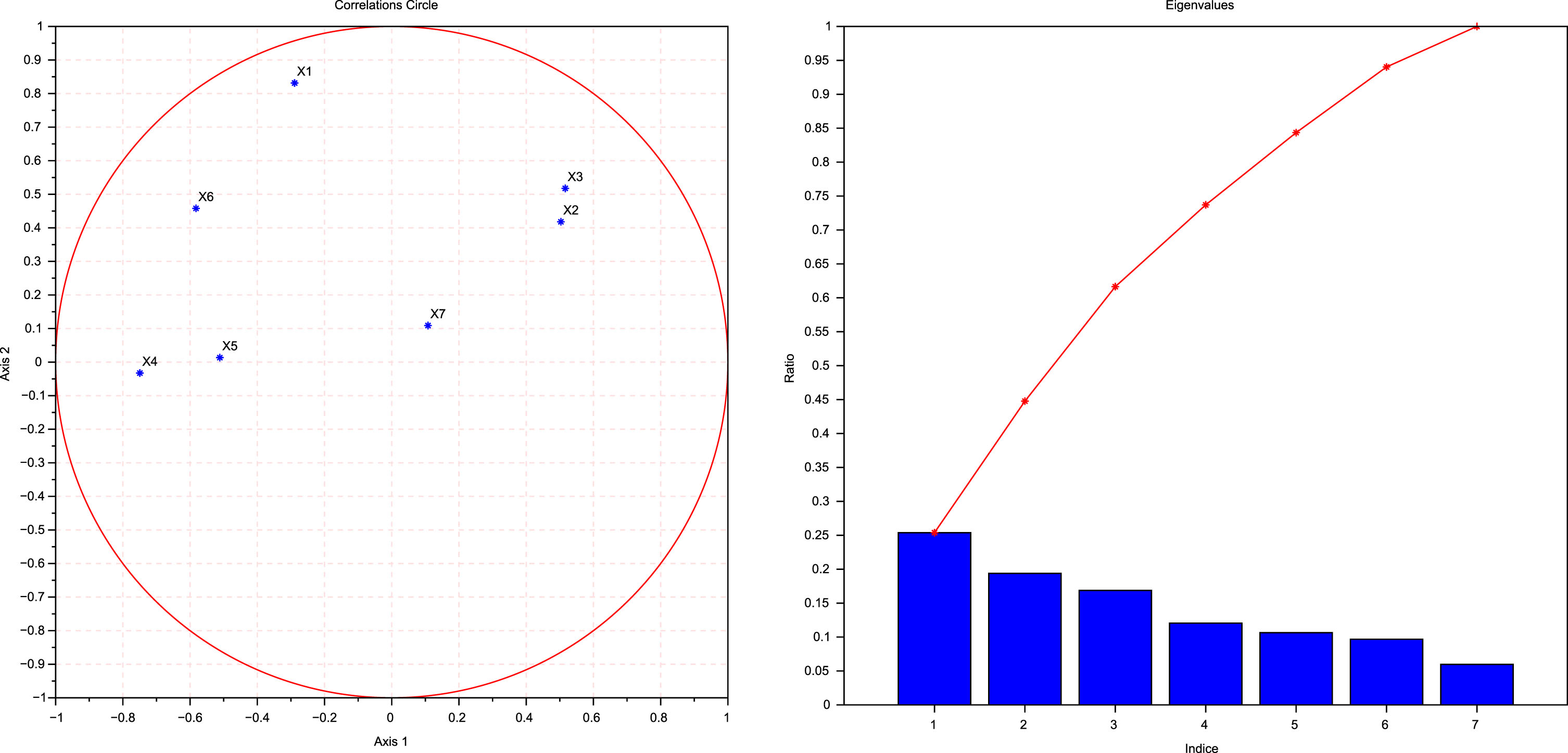
0.5233is the first column’s maximum value in absolute value. It is the coefficient of the first principal component with respect to variable number 6 which is the stock number 6. Thus, the first principal component has the largest positive association with the stock number 6. In other words, stock number 6 is the most dominating variable to the construction of the first factor.

0.6350is the second column’s maximum value in absolute value. It is the coefficient of the second principal component with respect to variable number 1 which is the stock number 1. Thus, the second principal component has the largest positive association with the stock number 1. In other words, stock number 1 is the most dominating variable for the construction of the second factor.

0.6250is the third column’s maximum value in absolute value. It is the coefficient of the third principal component with respect to variable number 5 which is the stock number 5. Thus, the third principal component has the largest positive association with the stock number 5. In other words, stock number 5 is the most dominating variable for the construction of the third factor.

0.5540is the fourth column’s maximum value in absolute value. It is the coefficient of the fourth principal component with respect to variable number 6 which is the stock number 6. Thus, the fourth principal component has the largest positive association with the stock number 6. In other words, stock number 6 is the most dominating variable in the construction of the fourth factor.

0.6942is the fifth column maximum’s value in absolute value. It is the coefficient of the fifth principal component with respect to variable number 3 which is the stock number 3. The fifth principal component has the largest positive association with the stock number 3. In other words, stock number 3 is the most dominating variable in the construction of the the fifth factor.

0.6478is the sixth column maximum’s value in absolute value. It is the coefficient of the sixth principal component with respect to variable 7 which is the stock number 7. The sixth principal component has the largest positive association with the stock number 7. In other words, stock number 7 is the most dominating variable in the construction of the sixth factor.

0.6543is the seventh column maximum value in absolute value. It is the coefficient of the seventh principal component with respect to variable 4 which is the stock number 4. The seventh principal component has the largest positive association with the stock number 4. In other words, stock number 4 is the most dominating variable in the construction of the seventh factor.

5.2.3 Derivation of the principal components

Define cfB₁, cfB₂, cfB₃, cfB₄, cfB₅, cfB₆ and cfB₇ to be the columns of cfB.

Then we have cfB = [cfB₁, cfB₂, cfB₃, cfB₄, cfB₅, cfB₆, cfB₇] which is the orthogonal matrix of the problem. cfB_i is the column number i of matrix cfB. In other words, cfB is a matrix containing all the elements of Table 4 except the first row and the first column of that table.

Define pcB_i i = 1, . . . , 7 to be the columns of the matrix pc containing the detailed principal components also called principal component analysis scores. Every pcB_i is vector of length equal to that of every original variable. we obtain the principal component analysis scores as follows: ${pcB}_{1} = \sum_{j = 1}^{7} cfB (j, 1) * Y_{j};$ (16) ${pcB}_{2} = \sum_{j = 1}^{7} cfB (j, 2) * Y_{j};$ (17) ${pcB}_{3} = \sum_{j = 1}^{7} cfB (j, 3) * Y_{j};$ (18) ${pcB}_{4} = \sum_{j = 1}^{7} cfB (j, 4) * Y_{j};$ (19) ${pcB}_{5} = \sum_{j = 1}^{7} cfB (j, 5) * Y_{j};$ (20) ${pcB}_{6} = \sum_{j = 1}^{7} cfB (j, 6) * Y_{j};$ (21) ${pcB}_{7} = \sum_{j = 1}^{7} cfB (j, 7) * Y_{j} .$ (22) In general we have

${pcB}_{k} = \sum_{j = 1}^{7} cfB (j, k) * Y_{j} .$ (23) where cfB (j, k)is the coefficient or component number j of the principal component pcB_k. It is the component of pcB_k with respect to the original variable number j which is Y_i.

The principal components pcB_k, j = 1, . . . , 7of the given dataset, are columns of pcB and stored in Table 3.

Each column of cfBcontains the coefficients for one principal component. Such columns are written in descending order of the variances that the components explain. Each principal component is a linear combination of the original variables. The principal component scores are stored in the matrix pcB. $pcB = [\begin{matrix} - 0.0367 & 0.2073 & 0.1793 & 0.0706 & 0.1255 & - 0.1395 & 0.1622 \\ 0.4380 & 0.1446 & 0.0999 & - 0.0237 & - 0.0755 & 0.0613 & - 0.1099 \\ - 0.0385 & 0.3730 & - 0.2976 & 0.1520 & - 0.0540 & - 0.1867 & 0.1417 \\ - 0.0736 & 0.3512 & - 0.2655 & - 0.0130 & - 0.1945 & - 0.0742 & 0.1158 \\ - 0.0077 & - 0.0836 & 0.0241 & 0.1404 & 0.2552 & 0.0045 & 0.0279 \\ - 0.1790 & - 0.4270 & - 0.0955 & 0.0744 & 0.0273 & 0.1035 & 0.0116 \\ 0.4013 & 0.0382 & - 0.0833 & - 0.0565 & 0.1221 & 0.1686 & 0.2321 \\ 0.1301 & - 0.2102 & 0.1876 & - 0.0940 & - 0.0272 & 0.1836 & 0.0137 \\ - 0.0037 & - 0.4131 & 0.0706 & - 0.1763 & - 0.1340 & - 0.1621 & 0.0392 \\ - 0.0741 & 0.1277 & 0.4566 & 0.1867 & - 0.0878 & 0.0220 & 0.0045 \\ 0.0196 & - 0.3649 & - 0.1342 & 0.1368 & 0.0119 & 0.0926 & 0.0814 \\ - 0.1802 & 0.0535 & - 0.0545 & - 0.1971 & 0.1313 & - 0.2107 & 0.0250 \\ 0.5381 & - 0.0023 & 0.1313 & 0.0602 & 0.0103 & - 0.1430 & 0.0252 \\ - 0.2967 & 0.0958 & 0.1615 & 0.0093 & - 0.0909 & 0.0324 & - 0.1918 \\ - 0.0279 & - 0.2138 & 0.0286 & - 0.1278 & 0.3243 & 0.0348 & 0.0564 \\ - 0.0874 & 0.0413 & - 0.0445 & - 0.2412 & 0.0713 & - 0.1412 & - 0.1242 \\ - 0.4827 & 0.2438 & - 0.0724 & - 0.1080 & 0.0537 & 0.2006 & - 0.0028 \\ 0.1738 & - 0.0379 & - 0.1378 & - 0.3151 & - 0.1916 & - 0.2000 & - 0.1523 \\ 0.3456 & 0.0434 & - 0.3003 & - 0.2532 & 0.1728 & 0.0965 & 0.0231 \\ - 0.2439 & - 0.2842 & - 0.0923 & 0.1938 & 0.1131 & - 0.2910 & - 0.0291 \\ 0.0199 & - 0.1745 & - 0.0035 & 0.0311 & - 0.1695 & - 0.2808 & - 0.0261 \\ - 0.0774 & - 0.1671 & 0.2319 & - 0.0790 & 0.1753 & 0.1188 & - 0.1850 \\ 0.1988 & - 0.0292 & - 0.2916 & 0.0170 & - 0.1962 & 0.2494 & - 0.0975 \\ - 0.2160 & 0.2799 & 0.0055 & - 0.1769 & - 0.0916 & 0.1288 & - 0.1293 \\ 0.0528 & 0.2883 & 0.0715 & - 0.0204 & 0.1305 & 0.1031 & 0.0363 \\ 0.0868 & - 0.0414 & 0.4529 & - 0.0787 & - 0.3114 & 0.0411 & 0.2197 \\ 0.0198 & 0.2419 & 0.0408 & 0.2642 & 0.2519 & - 0.0569 & - 0.1108 \\ - 0.6235 & - 0.1005 & - 0.0986 & - 0.0044 & - 0.1413 & 0.1366 & 0.1712 \\ 0.1455 & - 0.1862 & - 0.2928 & 0.4086 & - 0.1682 & 0.1186 & - 0.1094 \\ 0.0790 & 0.2059 & 0.1224 & 0.2201 & - 0.0427 & - 0.0106 & - 0.1190 \end{matrix}]$

One can obviously notice that they are linearly independent, orthogonal and generator of the vector space of dimension 7 on the real line. The variances that the principal components explain are stored in the vector λ_B.

$λ_{B} = [\begin{matrix} 0.0619 \\ 0.0501 \\ 0.0385 \\ 0.0280 \\ 0.0249 \\ 0.0225 \\ 0.0136 \end{matrix}]$ ∀i = 1, . . . , 7 we have the principal component pcB_i explain the variance represented by the eigenvalue λ_A (i). For example pcB₁ explains 25.85% of the total variation of the data.

The Hottelings T-squares statistic for each observation are as follows:

5.3224, 5.0771, 9.0640, 7.1351, 3.5359, 5.1076, 8.7438, 3.9244, 6.6498, 7.4036, 4.6746, 4.7577, 6.2109, 5.3660, 6.0453, 4.5116, 7.4065, 9.5139, 8.2515, 8.4744, 5.3549, 6.6486, 7.8785, 5.7396, 3.1049, 13.2194, 7.3085, 10.5162, 11.8674, 4.1862.

The percentage of total variance explained by each principal component are as follows:

$pcWeightsB = [\begin{matrix} 25.8568 \\ 20.9079 \\ 16.0893 \\ 11.6756 \\ 10.3870 \\ 9.4030 \\ 5.6804 \end{matrix}]$

From the above matrix one can see that the first principal component explains 25.9% of the variance of the data, the second explains 20.9%, the third explains 16.1%, the fourth explains11.7%, the fifth explains 10.4%, the sixth explains 9.4%, and the seventh explains5.7%. In general, the i^thprincipal component number explains percentage p of the total variance equal to ratio of the i^th(of the vector storing the eigenvalues) to the sum of all the eigenvalues.

The Hotelling T-Squared Statistic, which is the sum of squares of the standardized scores for each observation, returned as column vector. Hotellings T-Squared Statistic is a statistical measure of the multivariate distance of each observation from the center of data. Estimated means of each variable in D₂ is as follows.

$\begin{matrix} pcaMeans & = & [0.3593 0.3163 0.3760 0.3567 \\ 0.4150 0.3367 0.2997] \end{matrix}$ Some of the additional results are summarized by the following computational simulations:

Fig. 2

Computational simulations of Table 3.

Consider the first diagram of the computational simulations of Table 3: Axis 1 is for the first principal component while Axis 2 is for the second principal component. Each of the points x₁, x₂, x₃, x₄, x₅, x₆ and x₇ in that coordinate system axis are situated inside the correlation circle. ∀i = 1, 2, 3, 4, 5, 6, 7 we have x_i = (corr (pcB₁, stock_i) , corr (pcB₂, stock_i)) which can be expanded as follows: $x_{1} = (corr ({pcB}_{1}, Y_{1}), corr ({pcB}_{2}, Y_{1}))$ (24) $x_{2} = (corr ({pcB}_{1}, Y_{2}), corr ({pcB}_{2}, Y_{2}))$ (25) $x_{3} = (corr ({pcB}_{1}, Y_{3}), corr ({pcB}_{2}, Y_{3}))$ (26) $x_{4} = (corr ({pcB}_{1}, Y_{4}), corr ({pcB}_{2}, Y_{4}))$ (27) $x_{5} = (corr ({pcB}_{1}, Y_{5}), corr ({pcB}_{2}, Y_{5}))$ (28) $x_{6} = (corr ({pcB}_{1}, Y_{6}), corr ({pcB}_{2}, Y_{6}))$ (29) $x_{7} = (corr ({pcB}_{1}, Y_{7}), corr ({pcB}_{2}, Y_{7}))$ (30)

By reconsidering the results in Table 4, notice the resultant of all the principal components is also a linear combination of the original variables and is given by

-0.4294Y₁+ 0.245Y₂ + 0.9171Y₃ - 0.1318Y₄ +1.2578Y₅ + 1.9241Y₆ - 0.7801Y₇. Notice that before tackling this problem, the data of all the original variables were standardised, converted to a same scale and from this obtained resultant we see that the variable number 6 is the one having the maximum coefficient then we conclude that the stock number 6 is the dominating one in the portfolio.

5.2.4 Computation of the Portfolio Risk

Like the portfolio of the first dataset, this portfolio is represented by a multivariate time series of stocks. Every transaction of this portfolio is projected onto the space spanned by the principal components to give new transactions. The principal components are sufficient at this stage to compute the portfolio risk since they capture all the informations in an efficient manner. We do not need original variables to compute risk. New variables are sufficient to compute risk. Let Ω = (ω_i), i = 1, …, N be the proportion of stock i to be held in the portfolio π₂

$\begin{matrix} Risk (D_{2}) & = & \sum_{i = 1}^{7} \sum_{j = 1}^{7} ω_{i} Cov ({pcB}_{i}, {pcB}_{j}) \\ ω_{j} & = & \sum_{i = 1}^{7} Var ({pcB}_{i}) = \sum_{i = 1}^{7} λ_{B} (i) \end{matrix}$ (31) where Var (pcB_i) is the variance of the principal component number i, λ_B (i)is the eigenvalue number iof the second multivariate time series.

5.3 Application of the PCA on the third dataset

5.3.1 Introduction

The third given dataset D₃ is stored in Table 5. The rows of D₃ in Table 5 are the stock observations (the instantaneous stock rate of return vectors) and the columns are the data variables called stocks. By letting D₃ = [Z₁, Z₂, Z₃, Z₄, Z₅, Z₆, Z₇], we have that Zi = Stock_i ∀i = 1, . . . , 7. The columns of Table 5 are represented by the variables Z₁, Z₂, Z₃, Z₄, Z₅, Z₆ and Z₇. Each of them is a stock rate of return time series of length 30.

By letting D₃ = (R_ij) we have that R_ij is the rate of return at period i of stock j. Let Σ be the covariance matrix of D₃. It means that we have Σ = (cov (Z_i, Z_j)) , i, j = 1, . . . , 7. The eigenvectors of Σ are linearly independent and spanned a vector space of dimension equal to the number of the original variables which is 7. Their components represent the coefficients of the principal components (new variables) with respect to the original variables (the stocks). They are the columns and are stored in the matrix cfC.

The given dataset D₃ is stored in Table 5.

Table 5
Stock Returns during 30 months

Months Stock1 Stock2 Stock3 Stock4 Stock5 Stock6 Stock7

Janvier 0.5300 0.4600 0.4900 0.0500 0.0700 0.2800 0.3600

February 0.5900 0.0300 0.1700 0.0400 0.6300 0.0400 0.2000

March 0.0900 0.1800 0.3300 0.3500 0.0100 0.5900 0.4900

April 0.6000 0.0400 0.4600 0.5100 0.5100 0.6200 0.1300

May 0.4200 0.0700 0.5800 0.6100 0.5400 0.3200 0.4500

June 0.0700 0.5400 0.6300 0.0900 0.5700 0.3200 0.1200

July 0.1900 0.4600 0.3600 0.3700 0.0600 0.2200 0.2400

August 0.3600 0.2100 0.1000 0.3100 0.2600 0.5900 0.4100

September 0.6300 0.6200 0.1000 0.0100 0.1700 0.2500 0.5100

October 0.6300 0.0300 0.1700 0.2200 0.5300 0.0800 0.0600

November 0.1100 0.2900 0.5500 0.1100 0.2900 0.5100 0.6100

December 0.6400 0.2500 0.1700 0.5200 0.6000 0.2600 0.5100

January 0.6300 0.5000 0.5300 0.2100 0.1200 0.1600 0.3200

February 0.3200 0.5200 0.1600 0.3500 0.1800 0.2700 0.2900

March 0.5300 0.1300 0.6100 0.1100 0.1000 0.0700 0.3000

April 0.1000 0.3200 0.2300 0.4000 0.0900 0.0900 0.2000

May 0.2800 0.2900 0.1300 0.1800 0.5700 0.6200 0.3400

June 0.6000 0.4300 0.1700 0.4300 0.3800 0.6300 0.3400

July 0.5200 0.4700 0.4100 0.4500 0.3600 0.3800 0.5400

August 0.6300 0.5000 0.3100 0.4900 0.1000 0.0400 0.5200

September 0.4300 0.1800 0.2300 0.3000 0.5600 0.1600 0.4200

October 0.0300 0.4500 0.5500 0.0600 0.4100 0.2300 0.2500

November 0.5600 0.4300 0.3900 0.1500 0.2300 0.5400 0.5300

December 0.6100 0.1100 0.3600 0.6000 0.3400 0.0200 0.3500

January 0.4500 0.0800 0.6000 0.1000 0.2700 0.0300 0.2300

February 0.5000 0.3300 0.1900 0.5400 0.0500 0.1100 0.6200

March 0.4900 0.6300 0.5000 0.3500 0.1600 0.4300 0.5700

April 0.2600 0.2300 0.4900 0.6500 0.0900 0.4800 0.3600

May 0.4300 0.3900 0.2500 0.0600 0.1200 0.4300 0.4100

June 0.1200 0.1500 0.3700 0.2900 0.1600 0.3000 0.3900

Months	Stock1	Stock2	Stock3	Stock4	Stock5	Stock6	Stock7
Janvier	0.5300	0.4600	0.4900	0.0500	0.0700	0.2800	0.3600
February	0.5900	0.0300	0.1700	0.0400	0.6300	0.0400	0.2000
March	0.0900	0.1800	0.3300	0.3500	0.0100	0.5900	0.4900
April	0.6000	0.0400	0.4600	0.5100	0.5100	0.6200	0.1300
May	0.4200	0.0700	0.5800	0.6100	0.5400	0.3200	0.4500
June	0.0700	0.5400	0.6300	0.0900	0.5700	0.3200	0.1200
July	0.1900	0.4600	0.3600	0.3700	0.0600	0.2200	0.2400
August	0.3600	0.2100	0.1000	0.3100	0.2600	0.5900	0.4100
September	0.6300	0.6200	0.1000	0.0100	0.1700	0.2500	0.5100
October	0.6300	0.0300	0.1700	0.2200	0.5300	0.0800	0.0600
November	0.1100	0.2900	0.5500	0.1100	0.2900	0.5100	0.6100
December	0.6400	0.2500	0.1700	0.5200	0.6000	0.2600	0.5100
January	0.6300	0.5000	0.5300	0.2100	0.1200	0.1600	0.3200
February	0.3200	0.5200	0.1600	0.3500	0.1800	0.2700	0.2900
March	0.5300	0.1300	0.6100	0.1100	0.1000	0.0700	0.3000
April	0.1000	0.3200	0.2300	0.4000	0.0900	0.0900	0.2000
May	0.2800	0.2900	0.1300	0.1800	0.5700	0.6200	0.3400
June	0.6000	0.4300	0.1700	0.4300	0.3800	0.6300	0.3400
July	0.5200	0.4700	0.4100	0.4500	0.3600	0.3800	0.5400
August	0.6300	0.5000	0.3100	0.4900	0.1000	0.0400	0.5200
September	0.4300	0.1800	0.2300	0.3000	0.5600	0.1600	0.4200
October	0.0300	0.4500	0.5500	0.0600	0.4100	0.2300	0.2500
November	0.5600	0.4300	0.3900	0.1500	0.2300	0.5400	0.5300
December	0.6100	0.1100	0.3600	0.6000	0.3400	0.0200	0.3500
January	0.4500	0.0800	0.6000	0.1000	0.2700	0.0300	0.2300
February	0.5000	0.3300	0.1900	0.5400	0.0500	0.1100	0.6200
March	0.4900	0.6300	0.5000	0.3500	0.1600	0.4300	0.5700
April	0.2600	0.2300	0.4900	0.6500	0.0900	0.4800	0.3600
May	0.4300	0.3900	0.2500	0.0600	0.1200	0.4300	0.4100
June	0.1200	0.1500	0.3700	0.2900	0.1600	0.3000	0.3900

The rows of D₃ are the observations and the columns are the variables called stocks. The principal component coefficients for the given dataset X₃ are as stored in the matrix.

$\begin{matrix} cfC = \\ [\begin{matrix} 0.4633 & 0.5907 & - 0.1935 & - 0.3215 & 0.4241 & - 0.2419 & - 0.2392 \\ - 0.5048 & 0.2336 & - 0.2009 & - 0.3799 & 0.1179 & 0.6726 & - 0.1988 \\ - 0.1637 & - 0.3187 & - 0.1579 & 0.3781 & 0.8389 & 0.0061 & - 0.0034 \\ 0.1457 & 0.4625 & 0.4297 & 0.6342 & - 0.0043 & 0.3850 & - 0.1728 \\ 0.5590 & - 0.3380 & 0.3334 & - 0.3335 & 0.1912 & 0.4934 & 0.2664 \\ - 0.3366 & - 0.0315 & 0.7661 & - 0.3071 & 0.2061 & - 0.3013 & - 0.2667 \\ - 0.2381 & 0.4072 & 0.1205 & - 0.0405 & 0.1532 & - 0.0812 & 0.8551 \end{matrix}] \end{matrix}$

The above matrix can be rewritten as follows:

Each column of cfC contains the coefficients for one principal component. Such columns are in descending order of the component variances. Each principal component is a linear combination of the original variables. The principal component scores are stored in the matrix In Table 6 Z₁, Z₂, Z₃, Z₄, Z₅, Z₆ and Z₇ represent the original variables of the third input dataset and pcC₁, pcC₂, pcC₃, pcC₄, pcC₅, pcC₆ and pcC₇ are the new variables, the principal components.

Table 6

Eigenvectors

variables	pc₁	pc₂	pc₃	pc₄	pc₅	pc₆	pc₇
Z₁	0.4633	0.5907	-0.1935	-0.3215	0.4241	-0.2419	-0.2392
Z₂	-0.5048	0.2336	-0.2009	-0.3799	0.1179	0.6726	-0.1988
Z₃	-0.1637	-0.3187	-0.1579	0.3781	0.8389	0.0061	-0.0034
Z₄	0.1457	0.4625	0.4297	0.6342	-0.0043	0.3850	-0.1728
Z₅	0.5590	-0.3380	0.3334	-0.3335	0.1912	0.4934	0.2664
Z₆	-0.3366	-0.0315	0.7661	-0.3071	0.2061	-0.3013	-0.2667
Z₇	-0.2381	0.4072	0.1205	-0.0405	0.1532	-0.0812	0.8551

5.3.2 Interpretation of the eigenvector coefficients

From the results displayed in Table 6, one can notice the following:

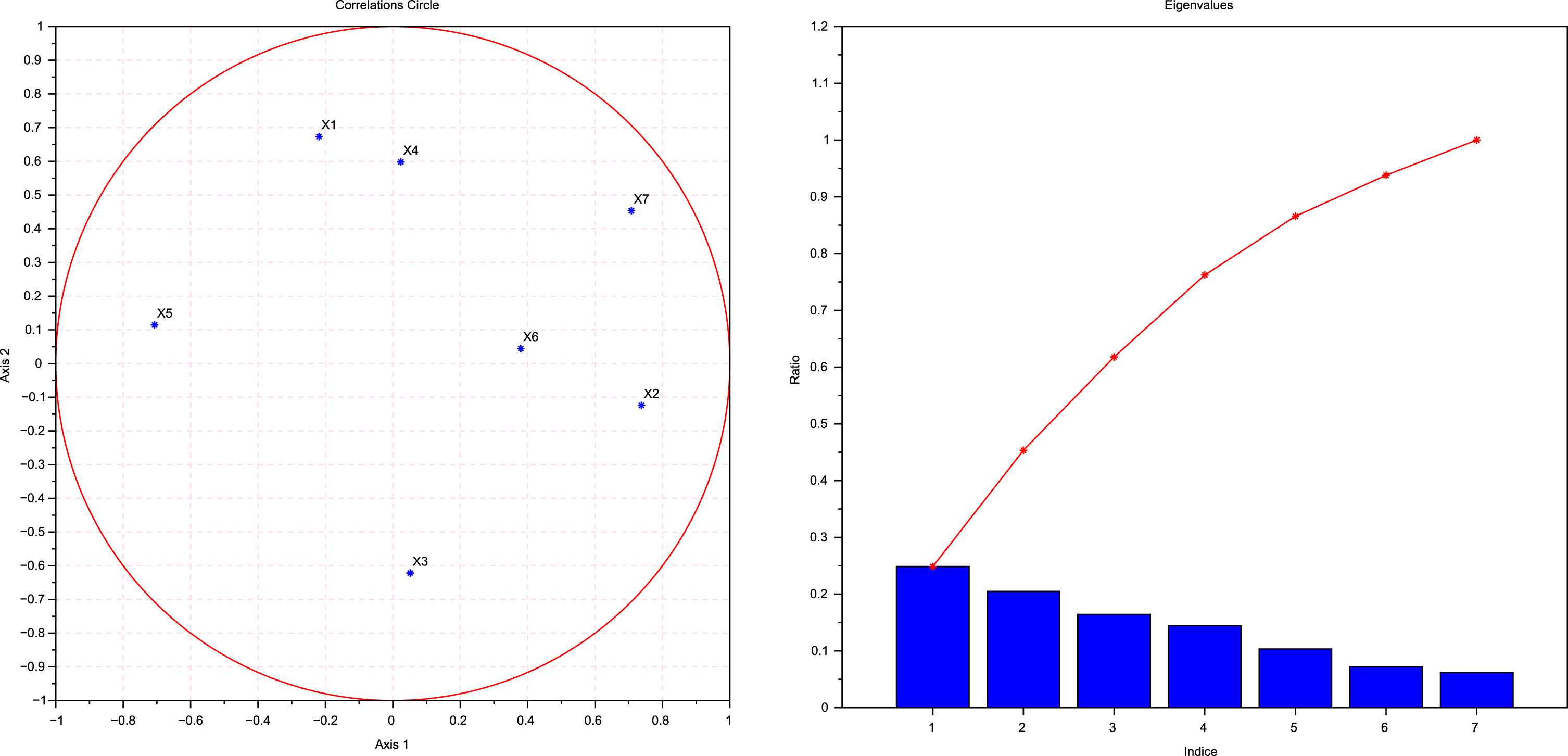
0.5590is the first column’s maximum value in absolute value. It is the coefficient of the first principal component with respect to variable number 5 which is the stock number 5. Thus, the first principal component has the largest positive association with the stock number 5. In other words, stock number 5 is the most dominating variable to the construction of the first factor.

0.5907is the second column’s maximum value in absolute value. It is the coefficient of the second principal component with respect to variable number 1 which is the stock number 1. Thus, the second principal component has the largest positive association with the stock number 1. In other words, stock number 1 is the most dominating variable for the construction of the second factor.

0.7661is the third column’s maximum value in absolute value. It is the coefficient of the third principal component with respect to variable number 6 which is the stock number 6. Thus, the third principal component has the largest positive association with the stock number 6. In other words, stock number 6 is the most dominating variable for the construction of the third factor.

0.6342is the fourth column’s maximum value in absolute value. It is the coefficient of the fourth principal component with respect to variable number 6 which is the stock number 4. Thus, the fourth principal component has the largest positive association with the stock number 4. In other words, stock number 4 is the most dominating variable in the construction of the fourth factor.

0.8389is the fifth column maximum’s value in absolute value. It is the coefficient of the fifth principal component with respect to variable number 3 which is the stock number 3. The fifth principal component has the largest positive association with the stock number 3. In other words, stock number 3 is the most dominating variable in the construction of the the fifth factor.

0.6726is the sixth column maximum’s value in absolute value. It is the coefficient of the sixth principal component with respect to variable 2 which is the stock number 2. The sixth principal component has the largest positive association with the stock number 2. In other words, stock number 2 is the most dominating variable in the construction of the sixth factor.

0.8551is the seventh column maximum value in absolute value. It is the coefficient of the seventh principal component with respect to variable 7 which is the stock number 7. The seventh principal component has the largest positive association with the stock number 7. In other words, stock number 7 is the most dominating variable in the construction of the seventh factor.

5.3.3 Derivation of the principal components

Define cfC₁, cfC₂, cfC₃, cfC₄, cfC₅, cfC₆ and cfC₇ to be the columns of cfC.

Then we have cfC = [cfC₁, cfC₂, cfC₃, cfC₄, cfC₅, cfC₆, cfC₇] which is the orthogonal matrix of the problem. cfC_i is the column number i of matrix cfC. In other words, cfC is a matrix containing all the elements of Table 4 except the first row and the first column of that table.

Define pcC_i i = 1, . . . , 7 to be the columns of the matrix pc containing the detailed principal components also called principal component analysis scores. Every pcC_i is vector of length equal to that of every original variable. we obtain the principal component analysis scores as follows: ${pcC}_{1} = \sum_{j = 1}^{7} cfC (j, 1) * Z_{j};$ (32) ${pcC}_{2} = \sum_{j = 1}^{7} cfC (j, 2) * Z_{j};$ (33) ${pcC}_{3} = \sum_{j = 1}^{7} cfC (j, 3) * Z_{j};$ (34) ${pcC}_{4} = \sum_{j = 1}^{7} cfC (j, 4) * Z_{j};$ (35) ${pcC}_{5} = \sum_{j = 1}^{7} cfC (j, 5) * Z_{j};$ (36) ${pcC}_{6} = \sum_{j = 1}^{7} cfC (j, 6) * Z_{j};$ (37) ${pcC}_{7} = \sum_{j = 1}^{7} cfC (j, 7) * Z_{j} .$ (38) In general we have

${pcC}_{k} = \sum_{j = 1}^{7} cfC (j, k) * Z_{j} .$ (39) where cfC (j, k)is the coefficient or component number j of the principal component pcC_k. It is the component of pcC_k with respect to the original variable number j which is Z_j.

The principal components pcC_k, j = 1, . . . , 7of the third given dataset, are columns of the matrix pcC.

Each column of cfCcontains the coefficients for one principal component. Such columns are written in descending order of the variances that the components explain. Each principal component is a linear combination of the original variables. The principal component scores are stored in the matrix pcC. $pcC = [\begin{matrix} - 0.1891 & 0.0164 & - 0.2703 & - 0.1209 & 0.1368 & - 0.1207 & - 0.0746 \\ 0.5386 & - 0.1982 & - 0.1658 & - 0.2107 & - 0.1237 & - 0.0687 & 0.0757 \\ - 0.3506 & - 0.0557 & 0.2584 & 0.1762 & - 0.1460 & - 0.2217 & 0.0475 \\ 0.3135 & - 0.0712 & 0.3824 & 0.0547 & 0.2088 & - 0.1099 & - 0.2574 \\ 0.2515 & - 0.0329 & 0.2539 & 0.2791 & 0.2291 & 0.0722 & 0.1237 \\ - 0.1366 & - 0.5308 & - 0.0338 & - 0.0944 & 0.1355 & 0.3147 & - 0.0706 \\ - 0.2356 & - 0.0386 & - 0.1103 & 0.1688 & - 0.1505 & 0.1068 & - 0.1374 \\ - 0.0500 & 0.0485 & 0.2930 & - 0.1144 & - 0.1852 & - 0.1538 & - 0.0172 \\ - 0.1353 & 0.2468 & - 0.2490 & - 0.4169 & - 0.0930 & - 0.0089 & 0.0408 \\ 0.5473 & - 0.1158 & - 0.1157 & - 0.0827 & - 0.1399 & - 0.0591 & - 0.1220 \\ - 0.3130 & - 0.2426 & 0.1411 & - 0.0147 & 0.1165 & - 0.0911 & 0.2601 \\ 0.3560 & 0.2342 & 0.1825 & - 0.0761 & 0.0084 & 0.1457 & 0.1355 \\ - 0.0684 & 0.1166 & - 0.3154 & - 0.0299 & 0.1955 & 0.0079 & - 0.1231 \\ - 0.1374 & 0.0849 & - 0.0402 & - 0.0415 & - 0.2150 & 0.1469 & - 0.1149 \\ 0.0683 & - 0.0992 & - 0.3553 & 0.1448 & 0.1516 & - 0.2359 & - 0.0071 \\ - 0.1109 & - 0.0915 & - 0.1257 & 0.2523 & - 0.3415 & 0.1024 & - 0.0844 \\ 0.0285 & - 0.1840 & 0.3497 & - 0.3000 & - 0.1292 & 0.0191 & 0.0231 \\ 0.0264 & 0.2045 & 0.3050 & - 0.2221 & 0.0212 & 0.0356 & - 0.1778 \\ - 0.0418 & 0.1954 & 0.1091 & - 0.0328 & 0.1686 & 0.1403 & 0.0615 \\ - 0.0099 & 0.4082 & - 0.2348 & 0.0999 & 0.0119 & 0.1244 & 0.0269 \\ 0.2849 & - 0.0470 & 0.0324 & - 0.0511 & - 0.0796 & 0.0828 & 0.1765 \\ - 0.1910 & - 0.4539 & - 0.1149 & - 0.0209 & 0.0117 & 0.1895 & 0.0549 \\ - 0.1677 & 0.1122 & 0.0617 & - 0.2337 & 0.1719 & - 0.1235 & 0.0259 \\ 0.3669 & 0.1905 & - 0.0690 & 0.2762 & 0.0146 & 0.0478 & 0.0140 \\ 0.1818 & - 0.2442 & - 0.3149 & 0.1378 & 0.1170 & - 0.1525 & 0.0199 \\ - 0.0327 & 0.4085 & - 0.0861 & 0.1838 & - 0.1440 & 0.0062 & 0.1371 \\ - 0.3016 & 0.2184 & 0.0008 & - 0.0632 & 0.2273 & 0.1010 & 0.0128 \\ - 0.1668 & 0.0676 & 0.2458 & 0.3657 & 0.0376 & - 0.0295 & - 0.1160 \\ - 0.1938 & 0.0208 & - 0.0571 & - 0.2113 & - 0.0671 & - 0.1658 & - 0.0216 \\ - 0.1315 & - 0.1678 & 0.0423 & 0.1981 & - 0.1494 & - 0.1024 & 0.0883 \end{matrix}]$

One can notice that they are linearly independent, orthogonal and generator of a vector space of dimension 7 on the real line. The principal component variances are store in the vector

$pcalatent 3 = [\begin{matrix} 0.0607 \\ 0.0485 \\ 0.0457 \\ 0.0363 \\ 0.0238 \\ 0.0176 \\ 0.0128 \end{matrix}]$

Fig. 3

Computational simulations of Table 5.

The Hottelings T-squares statistic for each observation are

4.6474, 8.7695, 8.2686, 12.7156, 8.3218, 13.1801, 5.0752, 5.1374, 8.1940, 7.8769, 9.6110, 6.7539, 5.3577, 4.7498, 7.7517, 8.5354, 6.6269, 6.8349, 3.7165, 5.8610, 4.5746, 7.4329, 4.4709, 5.3213, 6.3937, 6.8974, 5.3588, 6.7165, 3.7167, 4.1318.

The percentage of total variance explained by each principal component are stored in the vector

$pcaWeigths = [\begin{matrix} 24.7494 \\ 19.7606 \\ 18.6322 \\ 14.8100 \\ 9.6795 \\ 7.1677 \\ 5.2006 \end{matrix}]$

From the above matrix one can see that the first principal component explains 24.7% of the total variance of the data, the second explains 19.7%, the third explains 18.6%the fourth explains 14.8%the fifth explains9.7%the sixth, explains 7.2%, and the seventh explains 5.2%. The principal component number i explains an amount of percentage (of the total variance of the data) equal to the component number i of the vector storing the eigenvalues.

Consider the first diagram of the computational simulations of Table 5: Axis 1 is for the first principal component while Axis 2 is for the second principal component. Each of the points x₁, x₂, x₃, x₄, x₅, x₆ and x₇ in that coordinate system axis are situated inside the correlation circle. ∀i = 1, 2, 3, 4, 5, 6, 7 we have x_i = (corr (pcB₁, Z_i) , corr (pcB₂, Z_i)) which can be expanded as follows: $x_{1} = (corr ({pcC}_{1}, Z_{1}), corr ({pcC}_{2}, Z_{1}))$ (40) $x_{2} = (corr ({pcC}_{1}, Z_{2}), corr ({pcC}_{2}, Z_{2}))$ (41) $x_{3} = (corr ({pcC}_{1}, Z_{3}), corr ({pcC}_{2}, Z_{3}))$ (42) $x_{4} = (corr ({pcC}_{1}, Z_{4}), corr ({pcC}_{2}, Z_{4}))$ (43) $x_{5} = (corr ({pcC}_{1}, Z_{5}), corr ({pcC}_{2}, Z_{5}))$ (44) $x_{6} = (corr ({pcC}_{1}, Z_{6}), corr ({pcC}_{2}, Z_{6}))$ (45) $x_{7} = (corr ({pcC}_{1}, Z_{7}), corr ({pcC}_{2}, Z_{7}))$ (46)

By reconsidering the results in Table 6, notice the resultant of all the principal components is also a linear combination of the original variables and is given by

0.4820Z₁0.2603Z₂ + 0.5794Z₃ + 1.8800Z₄+1.1719Z₅ - 0.2710Z₆ + 1.1762Z₇. Notice that before tackling this problem, the data of all the original variables were standardised, converted to a same scale and from this obtained resultant we see that the variable number 4 is the one having the maximum coefficient then we conclude that the stock number 4 is the dominating one in the portfolio.

5.3.4 Computation of the portfolio risk

Like the portfolio of the first and the second datasets, this portfolio is represented by a multivariate time series of stocks. Every transaction of this portfolio is projected onto the space spanned by the principal components to give new transactions. The principal components are sufficient at this stage to compute the portfolio risk since they capture all the informations in an efficient manner. We do not need necessarily the original variables to compute risk. New variables are sufficient to compute risk. Let Ω = (ω_i), i = 1, …, N be the proportion of stock i to be held in the portfolio π₃. Then the risk is as follows:

$\begin{matrix} Risk (D_{3}) & = & \sum_{i = 1}^{7} \sum_{j = 1}^{7} ω_{i} Cov ({pcC}_{i}, {pcC}_{j}) \\ ω_{j} & = & \sum_{i = 1}^{7} Var ({pcC}_{i}) \sum_{i = 1}^{7} λ_{C} (i) \end{matrix}$ (47) where Var (pcC_i) is the variance of the principal component number i, λ_C (i)is the eigenvalue number iof the third multivariate time series.

6 Conclusion

The aim of this article was to apply principal component analysis to compute the main factors of the financial risk for each of the three considered portfolios, to extract the dominating stock for each computed factor of risk and for each portfolio and finally to compute the total risk for each portfolio. For each portfolio, the obtained eigenvalues of the covariance matrix determine the risks of the principal components which give the proportion of variance explained by the principal components. The associated eigenvector components determine how strong the principal components are connected to the original variables and determine the dominating variable for each main factor of risk. For each portfolio the dominating stock is determined. The Unsupervised Machine Learning technique used in this article involves notions of Linear Algebra, Multivariate Calculus, Probabilities, Mathematical Statistics and Algorithm development.

Footnotes

Acknowledgment

This work was supported by the University of Johannesburg.

References

Khan

, Farooq

, Principal component analysis-linear discriminant analysis, feature extractor for pattern recognition IJJCSIbas ed feature vector extraction, International Journal of Computer Science Issues 8(6), 2.

Murali

, 2015. Principal component analysis based feature vector extraction, Indian Journal of Science and Technology 8(35). Perlibakas,V., 2004. Distance measures for PCA-based face recognition, Pattern Recognition Letters 25, 711–724.

Perlibakas

, 2004. Distance measures for PCA-based face recognition, Pattern Recognition Letters 25, 711–724.

Wang

, Gao

, Nie

, 2017. Angle principal component analysis, Proceeding of the Twenty-sixth International Joint Conference on Artificial Intelligence (IJCAI-17), Main Track 2936–2942.

Zong

, Eurydice

, Galvasas

, 2014. Reconstruction undersample MR images by utilizing PCA pattern recognition, Journal of Basic Principle of Diffusion Theory, Experiment and Application, Diffusion-fundamentals.org22 14, 1–5.