Graph embedded dynamic mode decomposition for stock price prediction

Abstract

We present an algorithmic trading strategy based upon a graph version of the dynamic mode decomposition (DMD) model. Unlike the traditional DMD model which tries to characterize a stock’s dynamics based on all other stocks in a universe, the proposed model characterizes a stock’s dynamics based only on stocks that are deemed relevant to the stock in question. The relevance between each pair of stocks in a universe is represented as a directed graph and is updated dynamically. The incorporation of a graph model into DMD effects a model reduction that avoids overfitting of data and improves the quality of the trend predictions. We show that, in a practical setting, the precision and recall rate of the proposed model are significantly better than the traditional DMD and the benchmarks. The proposed model yields portfolios that have more stable returns in most of the universes we backtested.

Keywords

Trading strategy modeling asset price dynamics dynamical systems graph theory

1 Introduction

Stock price prediction is a very challenging problem in finance. Stock price series are non-linear, non-stationary, and dependant on a multitude of factors. To exploit market inefficiencies, we adopt a technical analysis approach, which tries to identify trading opportunities by analyzing statistical trends gathered from historical traded prices and volumes. Algorithms based on technical analysis are typically rooted in sophisticated statistical or mathematical models. Signal decomposition is an advanced data analysis technique, which identifies oscillating patterns at different time scales existed in time series. Commonly used decomposition methods include Fourier transform, dynamic mode decomposition (Rowley et al., 2009; Schmid & Sesterhenn 2008; Schmid, 2010; Kutz et al., 2000), empirical mode decomposition (Huang et al. 1971) and super empirical mode decomposition (Chui & Mhaskar, 2016). In this work, we adopt the dynamic mode decomposition (DMD) for its ability to extract the growth, decay, and oscillating rates of time series, which is very useful to the modeling of stock prices. Moreover, DMD is a spatial-temporal analysis tool that can be applied to multiple time series to identify the collective behaviours of multiple stocks.

Research on DMD is prolific; a lot of theories and extensions have been studied. We refer the readers to Kutz et al. (2000) and Schmid (2022) for thorough overviews of the subject. Originally proposed for the analysis of fluid mechanics, DMD is an effective method to extract low-dimensional non-linear dynamics of complex systems. It is an equation-free method which does not require the specification of a physical model. It adopts a data-driven approach to learn the dynamics of the system by extracting various modes and their growth and oscillation rates. It is proven to yield promising results in areas such as sociology, epidemiology, neuroscience, and physics (Centola & Macy 2007; Bullmore & Sporns 2009). In applications such as fluid mechanics, dynamics are governed by physical laws and some governing equations have been devised in many settings. But DMD can help when the existing models fail to capture the dynamics accurately in some situations.

The application of DMD in finance was pioneered by Mann & Kutz (2016) and Hua et al. (2016). As there are no governing equations for stock prices, data-driven approach becomes especially viable. In Mann & Kutz (2016), DMD is applied to predict prices of stocks in specific industry sectors, where some good results are found in the transportation, home construction, and retail sectors. The interesting notion of hotspots is introduced to guide the choice of the forecast horizon and the lookback period that lead to robust predictions. The results are obtained using several selected industry sectors with some small numbers of stocks (about 10). We, however, aim to develop a method that generates larger and more diversified portfolios from some generic pools of stocks. In Hua et al. (2016), DMD is used to extract cycles exhibited in the historical stock price time series that are robust to the sampling rate. DMD has also been used in Cui & Long (2016) and Kuttichira et al. (2017) to develop trading strategies and tested on different stock markets. They use the same method as in Mann & Kutz (2016) to produce predicted prices, but they differ in the generation of the trading signals (buy/sell/hold) from the predicted prices.

In this paper, we aim to further develop the DMD model in Mann & Kutz (2016), so that it can extract the trends of price series better and obtain portfolios that are more favourable. As stock markets are very dynamic, the good results obtained in backtests on small sectors are often non-reproducible in live trading. To this end, it is desirable to develop a model that can select stocks from some larger pools of stocks effectively. For example, stocks in a market index or smart beta Exchange-Traded Fund (ETF) are good candidates. Moreover, such stocks usually have large market capitalizations which make them less likely to be influenced a few major investors and are usually more liquid so that they are less likely to suffer from trading problems and large slippage. We find that if we directly apply the traditional DMD to universes of dozens of stocks, the recall rates (for upward trend predictions) are often low albeit their high precision rates. As a result, the number of selected stocks will be small and the portfolios constructed often exhibit high volatility and large drawdowns even in bull markets. This can be attributed to the problem of overfitting for the number of model parameters of DMD scales quadratically with the number of stocks. We therefore propose to embed a graph model into DMD to achieve a model reduction. We name the proposed model Graph Embedded Dynamic Model Decomposition (GEDMD). The method dynamically determines, for each stock, its most relevant stocks for predictions. Then the DMD technology is used to estimate the dynamics of the stock prices and make predictions. We find that the model can find stocks that are missed by the traditional DMD and construct portfolios that are more diversified and have more stable returns.

In Section 2, we present the DMD method for estimating the dynamics of multiple stocks. In Section 3, we present the proposed GEDMD method. The method consists of a graph construction procedure and a DMD-like optimization model. In Section 4, we present the experimental results to evaluate performance of the model in trading and the quality of the signals.

2 The dynamic mode decomposition

In this section, we describe the dynamic mode decomposition (DMD) method in a way convenient to the development of the proposed model presented in the next section. For other formulations and their deeper relations to the Koopman theory and system of differential equations, we refer the reader to Kutz et al. (2000).

Consider a universe comprising N stocks. Let t₁ < t₂ < ⋯ < t_M be the time points in a time window, in which the stock prices have been observed. Suppose that we would like to predict the price (or trend) at a future time, say t_M+τ. Denote by x _i (t_j) an L-dimensional feature vector for the i-th stock at the j-th time point, for i = 1, 2, …, N and for j = 1, 2, …, M. In general, although any set of features observable at or before t_j can be used for x _i (t_j), e.g. open, high, low, close, VWAP prices, volume, return and volatility at various time scales, we use the adjusted close prices over the L days at or before t_j as the feature vector x _i (t_j). The parameter L thus determines the lookback period for a prediction. The data is normalized so that the prices at time t_M are 1. In this way, predictions will be not be biased due to differences in the price range of different stocks. Owing to the normalization, the last entry of x _i (t_M) is 1 for each i. Specifically, let s_i (t_j) be the adjusted close price of the ith stock at time j, the feature vector for the ith stock at time t_j is given by $x_{i} (t_{j}) = [\begin{matrix} s_{i} (t_{j - L + 1}) / s_{i} (t_{M}) \\ s_{i} (t_{j - L + 2}) / s_{i} (t_{M}) \\ ⋮ \\ s_{i} (t_{j}) / s_{i} (t_{M}) \end{matrix}] .$ Note that the method treats t_M as the current time, where the stock prices s_i (t_j) for 2 - L ≤ j ≤ M have been observed, so that the construction of x _i (t_j) is possible. The data can be assembled into an LN × M matrix: $X = [\begin{matrix} x_{1} (t_{1}) & x_{1} (t_{2}) & \dots & x_{1} (t_{M}) \\ x_{2} (t_{1}) & x_{2} (t_{2}) & \dots & x_{2} (t_{M}) \\ ⋮ & ⋮ & ⋮ \\ x_{N} (t_{1}) & x_{N} (t_{2}) & \dots & x_{N} (t_{M}) \end{matrix}] .$ To learn a model for a forecast horizon of τ periods, we split the data matrix into two (overlapping) parts: $\begin{matrix} X_{1} & = & [\begin{matrix} x_{1} (t_{1}) & x_{1} (t_{2}) & \dots & x_{1} (t_{M - τ}) \\ x_{2} (t_{1}) & x_{2} (t_{2}) & \dots & x_{2} (t_{M - τ}) \\ ⋮ & ⋮ & ⋮ \\ x_{N} (t_{1}) & x_{N} (t_{2}) & \dots & x_{N} (t_{M - τ}) \end{matrix}] \\ X_{2} & = & [\begin{matrix} x_{1} (t_{1 + τ}) & x_{1} (t_{2 + τ}) & \dots & x_{1} (t_{M}) \\ x_{2} (t_{1 + τ}) & x_{2} (t_{2 + τ}) & \dots & x_{2} (t_{M}) \\ ⋮ & ⋮ & ⋮ \\ x_{N} (t_{1 + τ}) & x_{N} (t_{2 + τ}) & \dots & x_{N} (t_{M}) \end{matrix}] . \end{matrix}$ Let x (t_j) be the j-th column of the matrix X , i.e. $x (t_{j}) = [\begin{matrix} x_{1} (t_{j}) \\ x_{2} (t_{j}) \\ ⋮ \\ x_{N} (t_{j}) \end{matrix}] .$ The DMD method seeks an operator A (a square matrix of dimensions NL × NL) such that $A x (t_{j}) \approx x (t_{j + τ})$ (1) for j = 1, 2, …, M - τ. The operator A thus characterizes the dynamics of the system for the next τ periods of time. Equation (1) can also be expressed in terms of its block structure: $\begin{matrix} [\begin{matrix} A_{11} & A_{12} & \dots & A_{1 N} \\ A_{21} & A_{22} & \dots & A_{2 N} \\ ⋮ & ⋮ & ⋮ \\ A_{N 1} & A_{N 2} & \dots & A_{NN} \end{matrix}] \\ [\begin{matrix} x_{1} (t_{1}) & x_{1} (t_{2}) & \dots & x_{1} (t_{M - τ}) \\ x_{2} (t_{1}) & x_{2} (t_{2}) & \dots & x_{2} (t_{M - τ}) \\ ⋮ & ⋮ & ⋮ \\ x_{N} (t_{1}) & x_{N} (t_{2}) & \dots & x_{N} (t_{M - τ}) \end{matrix}] \\ \approx & [\begin{matrix} x_{1} (t_{1 + τ}) & x_{1} (t_{2 + τ}) & \dots & x_{1} (t_{M}) \\ x_{2} (t_{1 + τ}) & x_{2} (t_{2 + τ}) & \dots & x_{2} (t_{M}) \\ ⋮ & ⋮ & ⋮ \\ x_{N} (t_{1 + τ}) & x_{N} (t_{2 + τ}) & \dots & x_{N} (t_{M}) \end{matrix}] . \end{matrix}$ Each A _ij is an L × L matrix: $A_{ij} = [\begin{matrix} A_{ij} (1, 1) & A_{ij} (1, 2) & \dots & A_{ij} (1, L) \\ A_{ij} (2, 1) & A_{ij} (2, 2) & \dots & A_{ij} (2, L) \\ ⋮ & ⋮ & ⋮ \\ A_{ij} (L, 1) & A_{ij} (L, 2) & \dots & A_{ij} (L, L) \end{matrix}],$

which maps from the feature space of the j-th stock to the feature space of the i-th stock. The above model resembles the multivariate Markov chain model in Ching et al. (2002) and Ching et al. (2003), but the feature vectors in these work are probability distributions of states and the operator A consists of transition probabilities. It also has a close relationship to the vector autoregression model.

We remark that in Mann & Kutz (2016), Cui & Long (2016), Kuttichira et al. (2017), the feature vectors x _i (t_j) are 1-dimensional, consisting of the daily close price on the day t_j. This makes each prediction depend only on one day of close prices. But we found that using an L-dimensional feature vector to make each prediction depend on the prices over the last L days yields better results. The resulting data matrix X exhibits a Hankel structure, i.e. constant along the anti-diagonals. Such a Hankelization of data is well-known in the DMD community and has been used in many applications. It is also called the time-delayed coordinates in Kutz et al. (2000). From the point of view of ordinary differential equations or linear recurrence equations, Hankelization increases the order of the equations and the number of modes used to describe the dynamics.

We also remark that in Mann & Kutz (2016), Cui & Long (2016), Kuttichira et al. (2017), the horizon is set to τ = 1. To make a prediction of τ periods, the operator A is applied τ times to obtain x (t_j+τ) ≈ A ^τ x (t_j). However, in practice, most DMD modes estimated grow or decay exponentially with τ. Thus the predictions often deviate a lot from the actual stock prices as τ increases. We therefore set τ to the desired forecast horizon directly and make only a one-step prediction. This method is also known as the τ-DMD, studied in Prasadan & Nadakuditi (2020) in the context of blind source separation.

To obtain the operator A that fulfils Equation (1), a linear least-squares fitting is used: $A = \underset{A}{arg min} ∥ A X_{1} - X_{2} ∥_{F},$ where ∥ · ∥ _F denotes the Frobenius norm. This optimization problem has a closed-form solution of $A = X_{2} X_{1}^{†},$ where † denotes the Moore-Penrose pseudo-inverse of a matrix. If multiple solutions exist, the above solution is the one with the minimal Frobenius norm. The τ-period forecast $\hat{x} (t_{M + τ})$ can be obtained by $\hat{x} (t_{M + τ}) : = A x (t_{M}) = X_{2} X_{1}^{†} x (t_{M}) .$ As the prices are normalized such that the prices at t_M are 1, the prediction $\hat{x} (t_{M + τ})$ consists of the values 1 + r_i (h) for h = τ - L + 1, …, τ. Here, r_i (h) is the forecast of the h-day return for the i-th stock. The values 1 + r_i (τ) for i = 1, 2, …, N are extracted and used to generate trading signals.

In computational fluid dynamics, each x (t_j) is a snapshot of measurements on a 2D or 3D grid. Thus, to obtain a sufficient spatial resolution, x (t_j) usually has a very high dimensionality, whereas the number of snapshots M is usually much smaller. Moreover, researchers are often interested to inspect the eigenvectors and eigenvalues of the operator A to see the composition of the waveforms. As a result, they seldom compute A via $A = X_{2} X_{1}^{†}$ directly for the sake of efficiency. Instead, the following steps are performed to obtain the eigenvectors and eigenvalues:

Compute a reduced singular value decomposition (SVD) of X ₁ as: X ₁ = UΣV ^⊤;

Compute a similarity transform of A as: $\tilde{A} = U^{⊤} X_{2} V Σ^{- 1}$ ;

Compute an eigenvalue decomposition of $\tilde{A}$ as: $\tilde{A} = Φ Λ Φ^{- 1}$ ;

Obtain the eigenvectors and eigenvalues of A as: ΦU and Λ.

The idea here is that the matrix size of

\tilde{A}

is much smaller than that of A , so that the computational time is significantly reduced. Moreover, when DMD is applied in a rolling fashion (i.e. sliding time window), the SVD of X ₁ for a time window can be reused to obtain that for the next time window quickly. Furthermore, the rank of the matrix X ₁ can be adjusted via its SVD to achieve a low-rank approximation of the operator A , which can improve the model accuracy in some applications. However, in our application to finance, a practical universe usually consists of less than a thousand stocks and the number of lookback days L is usually a few dozen. As such, a direct computation of a prediction via

\hat{x} (t_{M + τ}) = X_{2} X_{1}^{†} x (t_{M})

is very fast with current hardware and linear algebra libraries. Specifically, we compute

y = X_{1}^{†} x (t_{M})

, followed by the multiplication X ₂ y . Moreover, as we will present in the next section, our model differs from the traditional DMD in that we solve the DMD problems of submatrices of A according to a graph structure, so that DMD is applied to matrices of much smaller sizes. Thus a direct computation is very efficient. Furthermore, the structure of A in our model is dynamically changing, so that an updating of the SVD of X ₁ is not possible. We remark that although we use daily close prices in our tests, it does not necessarily mean that in a live daily trading setting, we have many hours allowed for computation. For example, one may do the computation, make trading decisions, and place orders seconds before the market closes. This avoids delaying the orders to the next trading day. Thus a fast computation is vital in this scenario.

3 Graph embedded dynamic mode decomposition (GEDMD)

In the original DMD, the model (1) produces a prediction for a stock by combining the feature vectors of all stocks. For each stock, there are L²N unknown parameters in A to determine. It is therefore very easy to overfit the data in typical settings. If the universe consists of only a few stocks from related industries, then the overfitting problem may not be an issue. However, from the point of view of risk management, it is desirable to have a trading algorithm capable of selecting a diversified portfolio dynamically from a sizable pool of stocks.

The idea of the proposed method is very natural. In stock modeling, we expect the price of one stock to be more related to a small number of stocks from related industries than others. We first construct a directed graph that depicts the relevance of a stock in the prediction of the price of another stock. The construction method will be presented in the next subsection. Once a graph, represented with an adjacency matrix G , is obtained, we solve the DMD problem with the additional requirement that the operator A possesses a similar structure as G . The diagonal entries of G are set to be 1 to designate the dependence of a stock on its own historical prices. For illustration, consider a universe with N = 4 stocks and suppose that the adjacency matrix is estimated to be $G = [\begin{matrix} 1 & 0 & 1 & 0 \\ 0 & 1 & 1 & 1 \\ 1 & 0 & 1 & 0 \\ 1 & 0 & 0 & 1 \end{matrix}] .$ Then the operator A is required to have the block structure (i.e. sparsity pattern) of $A = [\begin{matrix} A_{11} & 0 & A_{13} & 0 \\ 0 & A_{22} & A_{23} & A_{24} \\ A_{31} & 0 & A_{33} & 0 \\ A_{41} & 0 & 0 & A_{44} \end{matrix}] .$ Here, each A _ij is an L × L matrix and 0 is the L × L zero matrix. For example, the prediction of x ₃ (t_M+τ) is given by ${\hat{x}}_{3} (t_{M + τ}) = A_{31} x_{1} (t_{M}) + A_{33} x_{3} (t_{M}) .$ The prediction depends only on the stocks deemed to be relevant to Stock 3 according to the third row of G . A model reduction is therefore effected. The key is the specification of the graph, which must be updated dynamically. We refer to the proposed model as the Graph Embedded Dynamic Mode Decomposition (GEDMD) model.

We note that the model in Salova et al. (2019) considers a block diagonal structure of A , whereas ours considers a generic block structure. We also note that in Jovanović et al. (2014), a sparsity-promoting DMD model is presented where the sparsity is imposed on the number of the modes. We, however, impose a sparsity criterion on the operator A which is very natural for stock predictions.

3.1 Graph Construction

The graphs that we use are unweighted, directed graphs with self-loops. We shall use the terms “graph” and “adjacency matrix” interchangeably. When selecting variables in regression algorithms, one often looks into the correlations between variables. Predictor variables that have little correlations to the response variable may be dropped, whereas predictor variables that are highly correlated may be compressed via dimension reduction techniques. It is therefore intuitive to rank the variables based on absolute correlations. In the analysis of time series of stock prices, it is common to calculate correlations based on the time series of daily simple return r_i (t_j) = s_i (t_j)/s_i (t_j-1) -1 or daily log-return r_i (t_j) = ln(s_i (t_j)/s_i (t_j-1)) Tsay (2010). Both kinds of return yield similar correlations, we use the daily simple return for its intuitive interpretation. In the prediction of a stock’s price, we use only its top k correlated stocks (including the stock itself) whose absolute correlations pass a test of statistical significance. Specifically, we determine the 99% confidence interval for each absolute correlation and require that the lower bound of the interval lies above a threshold c > 0, so that the interval is well above zero. For each stock, the number of selected stocks varies between 1 and k inclusively.

3.2 Mathematical Formulation

We present a formulation to embed a graph into DMD. For a given graph G , we define the set of neighbors (children) of Stock i to be $N (i) = {j : G_{ij} = 1}$ . The size of a neighborhood $N (i)$ is denoted by N_i. As mentioned in the beginning of Section 3, the DMD formulation we propose solves the problem $\underset{A}{arg min} ∥ A X_{1} - X_{2} ∥_{F}$ subject to constraints A _ij = 0 if G _ij = 0, where A _ij is an L × L block in A . The predictions are then given by $\hat{x} (t_{M + τ}) = A x (t_{M}) .$

In the rest of this subsection, we describe the main ideas of our method to solve the above minimization problem efficiently. In the next subsection, we will describe a regularized version to enhance the stability of the method. The regularized version is the ultimate method to propose, whose performance will be evaluated in the Section 4.

Consider Stock i and its neighbors $N (i)$ . Let the indices in $N (i)$ be $N (i) = {j_{1}, \dots, j_{N_{i}}}$ . Since A _ij = 0 for $j \notin N (i)$ , we have an equation in terms of a submatrix of A : $B^{(i)} X_{1}^{(i)} \approx X_{2}^{(i)},$ where $\begin{matrix} B^{(i)} & = & [\begin{matrix} A_{i, j_{1}} & A_{i, j_{2}} & \dots & A_{i, j_{N_{i}}} \end{matrix}], \\ X_{1}^{(i)} & = & [\begin{matrix} x_{j_{1}} (t_{1}) & x_{j_{1}} (t_{2}) & \dots & x_{j_{1}} (t_{M - τ}) \\ x_{j_{2}} (t_{1}) & x_{j_{2}} (t_{2}) & \dots & x_{j_{2}} (t_{M - τ}) \\ ⋮ & ⋮ & ⋮ \\ x_{j_{N_{i}}} (t_{1}) & x_{j_{N_{i}}} (t_{2}) & \dots & x_{j_{N_{i}}} (t_{M - τ}) \end{matrix}], \\ X_{2}^{(i)} & = & [\begin{matrix} x_{i} (t_{1 + τ}) & x_{i} (t_{2 + τ}) & \dots & x_{i} (t_{M}) \end{matrix}] . \end{matrix}$ The least-squares solution is given by $B^{(i)} = X_{2}^{(i)} (X_{1}^{(i)})^{†}$ and the prediction for Stock i is given by ${\hat{x}}_{i} (t_{M + τ}) = B^{(i)} x^{(i)} (t_{M}),$ (2) where $x^{(i)} (t_{M}) = [\begin{matrix} x_{j_{1}} (t_{M}) \\ x_{j_{2}} (t_{M}) \\ ⋮ \\ x_{j_{N_{i}}} (t_{M}) \end{matrix}] .$ Equation (2) is computed for each i to obtain the predictions for every stocks. The computation for different stocks can be parallelized. However, the neighborhood of a stock varies with time, so that the computed B ⁽ⁱ⁾ for one time step cannot be reused to update the next B ⁽ⁱ⁾.

3.3 Tikhonov Regularization

The stability of the minimization problem $min_{B^{(i)}} ∥ B^{(i)} X_{1}^{(i)} - X_{2}^{(i)} ∥_{2}$ is dictated by the condition number of $X_{1}^{(i)}$ , where the condition number is given by the ratio of the largest singular value to the smallest (non-zero) singular value of $X_{1}^{(i)}$ . In our experiments, we do not find the minimization problem based on real stock price data very ill-conditioned. However, to enhance the stability of the method, we adopt the following Tikhonov regularization (Tikhonov & Arsenin 1977): $min_{B^{(i)}} {∥ B^{(i)} X_{1}^{(i)} - X_{2}^{(i)} ∥_{2}^{2} + λ ∥ B^{(i)} ∥_{2}^{2}},$ (3) where λ > 0 is the regularization parameter, chosen to maintain the condition number to roughly 100. The regularized minimization problem can be solved efficiently by first computing the reduced SVD of $X_{1}^{(i)}$ as $X_{1}^{(i)} = \hat{U} \hat{Λ} {\hat{V}}^{⊤}$ , followed by setting $B^{(i)} = X_{2}^{(i)} \hat{V} {(\hat{Λ} + λ {\hat{Λ}}^{- 1})}^{- 1} {\hat{U}}^{⊤} .$

We remark that a few other regularized DMD methods have been studied. They include Dicle et al. (2016), Takeishi et al. (2017), and Schmid (2022).

4 Experiments

We test the proposed GEDMD model in two different aspects: 1) signal quality (precision and recall rates), and 2) trading performance. We compare the performance of GEDMD with DMD and some benchmarks. We also demonstrate the effectiveness of the regularization used.

4.1 Investment Objectives

While making profits is the ultimate investment goal, we view the GEDMD model as a basic tool used to form a part of a larger portfolio, and therefore, we evaluate the model on various aspects besides the return. Fund managers need different tools in different market conditions and to cater the risk appetite of different investors. Tools that can generate small but steady excess incomes are valuable. Specifically, if a model can generate an excess return over an off-the-shelf liquid traded instrument consistently over time, then the two instruments can form a hedged pair to generate positive incomes. It is also comfortable to leverage it to boost the return. On the other hand, models that show very high returns in backtests often bet on a small number of stocks and thus may suffer from concentration risks. Such models can be attractive at times, but the capital allocation should be exercised with caution, not to mention leveraging.

4.2 Datasets

In view of the aforementioned investment objectives, we test the performance of GEDMD with the eleven GICS industrial sectors of the S&P 500 index. Their underlying stocks make up the S&P 500 index and thus they represent the US market well. These sectors can be traded via exchange-traded funds (ETFs) which are summarized in Table 1. For each of these eleven universes, we compare the ETF (the benchmark) with DMD and GEDMD applied to the underlying stocks of the ETF. These ETFs have large capitalizations and are liquid, making them good candidates for comparison. For evaluation purposes, all the eleven universes are used. But the energy sector is volatile and consists of only a small number of stocks. So, trading on this universe exhibits high uncertainty. In fact, the ETF, which tracks the sector index, has only a 1% return in 2019–2021, see Table 1. We also do not filter the stocks, which may introduce biases.

Table 1
Universes used in the experiments. The underlying stocks are as of 11/16/2021. The returns are for the period from 1/1/2019 to 11/15/2021

Item Symbol Description No. stocks Return (%)

1 XLB Materials Select Sector SPDR ETF 28 65.71

2 XLC Communication Services Sel Sect SPDR ETF 27 92.02

3 XLE Energy Select Sector SPDR ETF 22 0.97

4 XLF Financial Select Sector SPDR ETF 65 64.49

5 XLI Industrial Select Sector SPDR ETF 74 58.93

6 XLK Technology Select Sector SPDR ETF 73 151.39

7 XLP Consumer Staples Select Sector SPDR ETF 32 40.27

8 XLRE Real Estate Select Sector SPDR 29 52.53

9 XLU Utilities Select Sector SPDR ETF 28 26.28

10 XLV Health Care Select Sector SPDR ETF 64 51.18

11 XLY Consumer Discretionary Select Sector SPDR ETF 63 89.46

Item	Symbol	Description	No. stocks	Return (%)
1	XLB	Materials Select Sector SPDR ETF	28	65.71
2	XLC	Communication Services Sel Sect SPDR ETF	27	92.02
3	XLE	Energy Select Sector SPDR ETF	22	0.97
4	XLF	Financial Select Sector SPDR ETF	65	64.49
5	XLI	Industrial Select Sector SPDR ETF	74	58.93
6	XLK	Technology Select Sector SPDR ETF	73	151.39
7	XLP	Consumer Staples Select Sector SPDR ETF	32	40.27
8	XLRE	Real Estate Select Sector SPDR	29	52.53
9	XLU	Utilities Select Sector SPDR ETF	28	26.28
10	XLV	Health Care Select Sector SPDR ETF	64	51.18
11	XLY	Consumer Discretionary Select Sector SPDR ETF	63	89.46

The backtests are done for the period of 1/1/2019 to 11/15/2021. Time series of adjusted daily close prices are used. To examine the effects of introducing a graph structure into DMD, we compare GEDMD with the traditional DMD using a fixed set of parameters of τ = 20, L = 30, and M = 120. The parameters are set for practical reasons. In trading, a holding period of 1 month (approximately 20 trading days) allows for a predicted trend to develop. A shorter period may only reflect the volatility of the stocks. It is also desirable to rebalance portfolios monthly. In our experience, predictions with longer horizons using DMD-type methods often lead to poorer results as the dynamics are heterogenous.

4.3 Signal Quality

To understand the behaviour of the models, we study the quality of the predictions in terms of precision and recall rates. The recall and precision rates are defined by $recall = \frac{TP}{TP + FN} precision = \frac{TP}{TP + FP}$ where TP is the number of true positives, FN is the number of false negatives, and FP is the number of false positives. An upward trend (return higher than the threshold) is considered positive. For GEDMD and DMD, a stock is classified to be UP if the predicted return exceeds the threshold, which we will vary from 1% to 10%. The “baseline” prediction is the trivial one that all stocks are predicted UP.

The average recall rates for the universes and the respective standard deviations are reported in Table 2. The GEDMD yields higher recall rates than the DMD across all thresholds. This indicates that GEDMD captures a larger number of stocks with an uptrend. This helps in the diversification of the portfolios. Notice that even if a prediction is deemed “wrong”, it may still generate a positive return. Readers are referred to Table 4 for the actual returns.

Table 2
Performance statistics: Average recall for the universes (%). The respective standard deviations are shown in the brackets

Threshold GEDMD DMD

1 48.44 (5.88) 45.48 (4.34)

2 43.00 (5.38) 38.08 (5.01)

3 38.19 (5.25) 30.84 (5.34)

4 34.20 (4.55) 25.03 (5.82)

5 30.66 (4.27) 20.20 (6.38)

6 28.34 (4.49) 15.98 (7.20)

7 25.94 (4.68) 13.53 (7.57)

8 23.53 (4.93) 10.47 (7.65)

9 21.79 (5.35) 8.93 (7.94)

10 20.70 (5.46) 6.96 (7.48)

Threshold	GEDMD	DMD
1	48.44 (5.88)	45.48 (4.34)
2	43.00 (5.38)	38.08 (5.01)
3	38.19 (5.25)	30.84 (5.34)
4	34.20 (4.55)	25.03 (5.82)
5	30.66 (4.27)	20.20 (6.38)
6	28.34 (4.49)	15.98 (7.20)
7	25.94 (4.68)	13.53 (7.57)
8	23.53 (4.93)	10.47 (7.65)
9	21.79 (5.35)	8.93 (7.94)
10	20.70 (5.46)	6.96 (7.48)

The average precision for the universes and the respective standard deviations are reported in Table 3. The baseline gives the prior distribution of the uptrend stocks. We see that the GEDMD yields higher precisions than the DMD and the baseline when the threshold is 5% or larger. However, when the threshold is lower than 5%, the precisions of the different methods are close. This is reasonable because a small predicted return is comparable to the intrinsic volatility of the stock. The standard deviations of GEDMD agree with that of the basline, showing the inherent variability among the universes. Note that the precisions give the probability of making a correct prediction. We will see in the trading experiments that the improved precision of GEDMD leads to an attractive excess return over the baseline when the portfolio involves hundreds of trades (predicted positives) over three years.

Table 3

Performance statistics: Average precision for the universes (%). The respective standard deviations are shown in the brackets

Threshold	GEDMD	DMD	Baseline
1	50.72 (4.70)	51.68 (4.53)	53.69 (3.29)
2	45.31 (5.23)	45.56 (5.49)	48.08 (3.88)
3	40.69 (4.83)	39.79 (5.66)	42.61 (3.94)
4	36.86 (4.09)	34.63 (6.45)	37.04 (3.87)
5	33.41 (3.50)	31.04 (7.79)	32.09 (4.22)
6	30.45 (4.09)	26.55 (9.83)	27.35 (4.54)
7	27.95 (4.28)	25.08 (10.52)	23.57 (4.53)
8	25.46 (4.24)	21.89 (12.75)	20.46 (4.62)
9	22.84 (4.81)	20.94 (13.88)	17.30 (4.65)
10	20.95 (4.92)	17.81 (13.21)	14.81 (4.37)

4.4 Trading Performance

In this subsection, portfolios of stocks from a universe are formed and are rebalanced monthly. On each rebalancing day, the models select stocks that are predicted to have an upward trend for the next period of time. A stock is classified as “UP” if the predicted return is higher than a threshold, which we will vary from 1% to 10%. The selected stocks will take long positions and will be held until the next rebalancing day. We trade only the long positions because in practice short positions are sometimes difficult to fully fill timely. All available capital will be invested/reinvested. The capital will be equally divided among the selected stocks. No stop-loss or take-profit rules are used.

In production, additional measures such as setting entry price limits, stop-loss, take-profit, capital allocation, and portfolio weights optimization should be taken. The choice of these rules can significantly affect the performance. To investigate the performance due to the GEDMD and DMD predictions, we isolate factors due to trading rules.

To avoid overwhelming with many statistics and to provide more reliable statistics, the average returns for the universes and the respective standard deviations are reported in Table 4. The GEDMD yields higher returns than the DMD and the benchmark across all thresholds. The return of GEDMD also shows in increasing trend with the threshold. This indicates that stocks that have a high predicted return (e.g. 10%) exhibit a stronger upward trend and are more likely to yield a positive return than stocks that have a low predicted return (e.g. 1%). When the threshold is 10%, the excess return of GEDMD is about 26.0%, annualized to 8.6%, which is quite good for such a diversified portfolio. The return of DMD does not show an increasing trend. This is related to the number of selected stocks and the low recall rate. The standard deviations reflect the diversity of the performance of the universes. GEDMD exhibits a slight increasing trend of the standard deviation with the return, which is the usual trade-off between return and risk. But we will see in Table 5 that the Sharpe ratios remain steady.

Table 4
Performance statistics: Average return (standard deviation) for the universes (%). The respective standard deviations are shown in the brackets

Threshold GEDMD DMD Benchmark

(%)

1 70.26 (39.36) 58.73 (35.69) 63.02 (39.17)

2 70.68 (39.13) 62.01 (40.83) 63.02 (39.17)

3 72.32 (39.85) 51.85 (39.24) 63.02 (39.17)

4 75.82 (40.58) 49.59 (44.93) 63.02 (39.17)

5 74.98 (40.34) 48.88 (41.52) 63.02 (39.17)

6 71.35 (44.49) 52.92 (75.65) 63.02 (39.17)

7 77.45 (47.83) 53.04 (65.70) 63.02 (39.17)

8 79.21 (49.17) 57.03 (96.34) 63.02 (39.17)

9 83.67 (55.83) 68.31 (119.19) 63.02 (39.17)

10 89.01 (55.30) 55.79 (70.19) 63.02 (39.17)

Threshold	GEDMD	DMD	Benchmark
1	70.26 (39.36)	58.73 (35.69)	63.02 (39.17)
2	70.68 (39.13)	62.01 (40.83)	63.02 (39.17)
3	72.32 (39.85)	51.85 (39.24)	63.02 (39.17)
4	75.82 (40.58)	49.59 (44.93)	63.02 (39.17)
5	74.98 (40.34)	48.88 (41.52)	63.02 (39.17)
6	71.35 (44.49)	52.92 (75.65)	63.02 (39.17)
7	77.45 (47.83)	53.04 (65.70)	63.02 (39.17)
8	79.21 (49.17)	57.03 (96.34)	63.02 (39.17)
9	83.67 (55.83)	68.31 (119.19)	63.02 (39.17)
10	89.01 (55.30)	55.79 (70.19)	63.02 (39.17)

Table 5

Performance statistics: Average Sharpe ratio (standard deviation) for the universes. The respective standard deviations are shown in the brackets

Threshold (%)	GEDMD	DMD	Benchmark
1	0.91 (0.36)	0.84 (0.47)	0.86 (0.34)
2	0.91 (0.37)	0.87 (0.47)	0.86 (0.34)
3	0.92 (0.39)	0.65 (0.42)	0.86 (0.34)
4	0.94 (0.40)	0.61 (0.41)	0.86 (0.34)
5	0.89 (0.39)	0.64 (0.49)	0.86 (0.34)
6	0.85 (0.42)	0.63 (0.47)	0.86 (0.34)
7	0.90 (0.43)	0.67 (0.38)	0.86 (0.34)
8	0.92 (0.41)	0.58 (0.54)	0.86 (0.34)
9	0.93 (0.45)	0.69 (0.57)	0.86 (0.34)
10	0.95 (0.43)	0.69 (0.65)	0.86 (0.34)

The average Sharpe ratios for the universes and the respective standard deviations are reported in Table 5. The GEDMD yields higher Sharpe ratios than the DMD across all thresholds and the baseline in 9 of the 10 thresholds. Thus, GEDMD is able to select stocks in a universe dynamically to improve the Sharpe ratio of the universe. The Sharpe ratio of GEDMD is quite robust to the threshold. The DMD shows a higher variability in the statistic.

To see the performance on the individual universes, the average returns for the thresholds are depicted in Table 6 universe. The GEDMD outperforms the DMD in 8 of the 11 universes and outperforms the baseline in 7 of the 11 universes. The DMD gives outstanding returns in XLE (energy) and XLY (consumer discretionary).

Table 6

Performance statistics: Average return for the thresholds (%). The respective standard deviations are shown in the brackets. GEDMD has the highest excess return in XLV. DMD has the highest excess return in XLY

Universe	GEDMD	DMD	Benchmark
XLB	101.77 (17.57)	70.03 (33.58)	65.71
XLC	76.35 (12.71)	14.45 (19.33)	92.02
XLE	16.83 (16.44)	45.90 (25.97)	0.97
XLF	83.88 (11.81)	28.56 (18.25)	64.49
XLI	92.78 (2.57)	70.74 (51.25)	58.93
XLK	163.86 (20.58)	82.05 (32.44)	151.39
XLP	36.36 (7.53)	18.41 (18.45)	40.27
XLRE	44.47 (11.08)	61.28 (13.86)	52.53
XLU	20.25 (8.29)	-0.22 (7.77)	26.28
XLV	102.53 (7.59)	25.61 (19.17)	51.18
XLY	102.15 (21.85)	197.15 (112.93)	89.46

To compare the portfolios on a daily basis, we choose XLV and XLY to illustrate. The GEDMD and DMD have the highest excess returns over the benchmark in XLV and XLY, respectively. The portfolio values (per dollar initial investment) are shown in Fig. 1 and Fig. 2.

Fig. 1

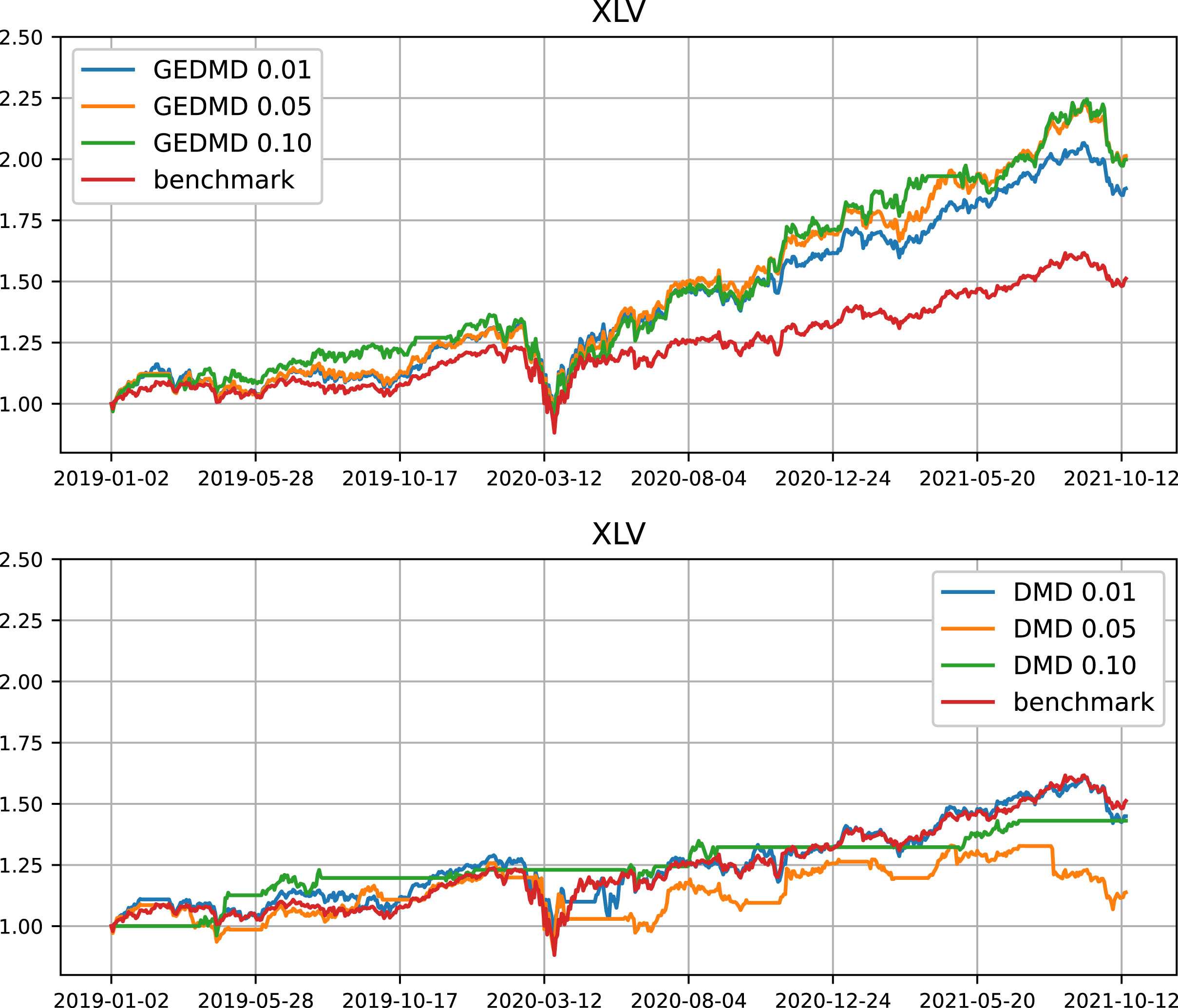
Trading performance in the XLV universe. Portfolio value per unit initial investment. This universe is chosen in favour of GEDMD. Note that GEDMD outperforms DMD in 8 of the 11 universes.

Fig. 2

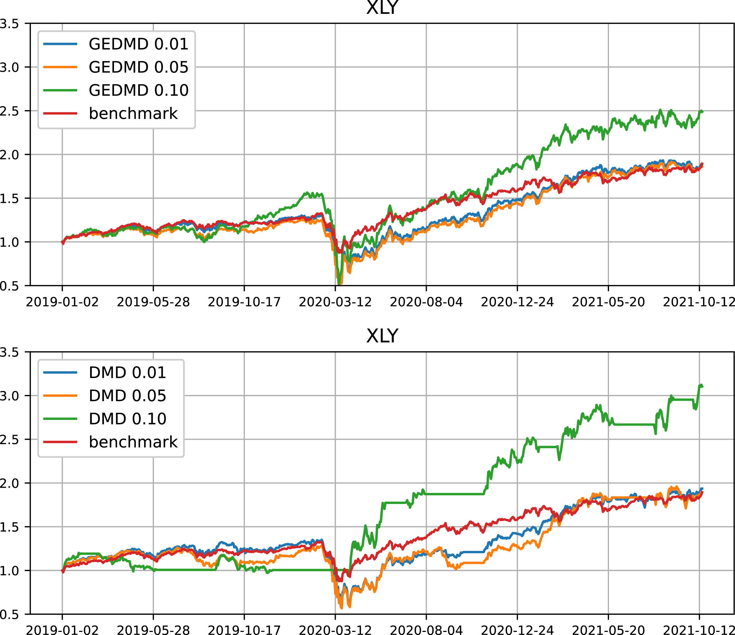
Trading performance in the XLY universe. Portfolio value per unit initial investment. This universe is chosen in favour of DMD. Note that GEDMD outperforms DMD in 8 of the 11 universes.

In Fig. 1, the GEDMD yields very consistent excess returns over time. The results are also robust to the choice of the threshold. The portfolios generally dropped during the market crash in 2020Q1 due to covid-19. Such infrequent black-swan events cannot be predicted with the models. Trading rules such as stop-loss should be imposed to limit the loss, but as mentioned above, it is not our purpose to study trading rules in this paper. The performance of DMD in the XLV universe is poor. With a threshold of 1%, it follows closely with the benchmark, meaning that most of the stocks in the universe are selected. With a threshold of 10%, there are many flat regions, indicating that no stocks are selected even though XLV has 64 stocks. The investment is halted for excessive long periods and has avoided the down markets. It reaches the same final return as the benchmark at the end. But it puts the capital into a very small number of stocks. There are only trades 33 times during the 3-year period.

Fig 2 shows a good case of DMD. For DMD, with a threshold of 1% and 5%, the performance is similar to the GEDMD and the benchmark. However, with a threshold of 10%, the return increases significantly. This is again due to the concentration on a small number of stocks. For example, in April 2019, DMD selects only one stock, namely, Align. This stock has a prolonged uptrend prior to April 2019 and is detected by DMD. We also see that the portfolio value is doubled in 2020Q2. But this kind of behaviour does not occur in all 11 universes. It is important to consider the average behaviour too. For GEDMD, it has a large drawdown in 2020Q1 and a pronounced rebound afterwards. The capital is indeed quintupled from $0.5 to $2.5.

4.5 Effect of Regularization

To demonstrate the effectiveness of the regularization in Equation (3), we show the daily condition number of the least-squares problem for the XLV and the XLY universes in Fig. 3. For comparison purposes, we also include the condition number of the truncated SVD regularization, which is another commonly used regularization method. In truncated SVD, singular values of $X_{1}^{(i)}$ less than a threshold η are truncated in the computation of $(X_{1}^{(i)})^{†}$ . The threshold η is determined so that 1) the resulting portfolio returns are similar to that of the Tikhonov method, and 2) the threshold η is as large as possible to enhance the stability. For example, the returns of GEDMD shown in Table 4 have a mean absolute difference of 3.1% between the two regularization methods. We observe in Fig. 3 that the condition number of Tikhonov is stabilized around 100. The condition number increases to about 260 after the market crash due to the presence of larger values in the data matrix $X_{1}^{(i)}$ but it remains under control. The condition number of truncated SVD fluctuates between 2000 and 4000. Despite the increased condition number of truncated SVD, the portfolio returns are similar. This is because the predicted returns are dichotomized into UP or DOWN only. Having said so, it is desirable to work with a method having a smaller condition number.

Fig. 3

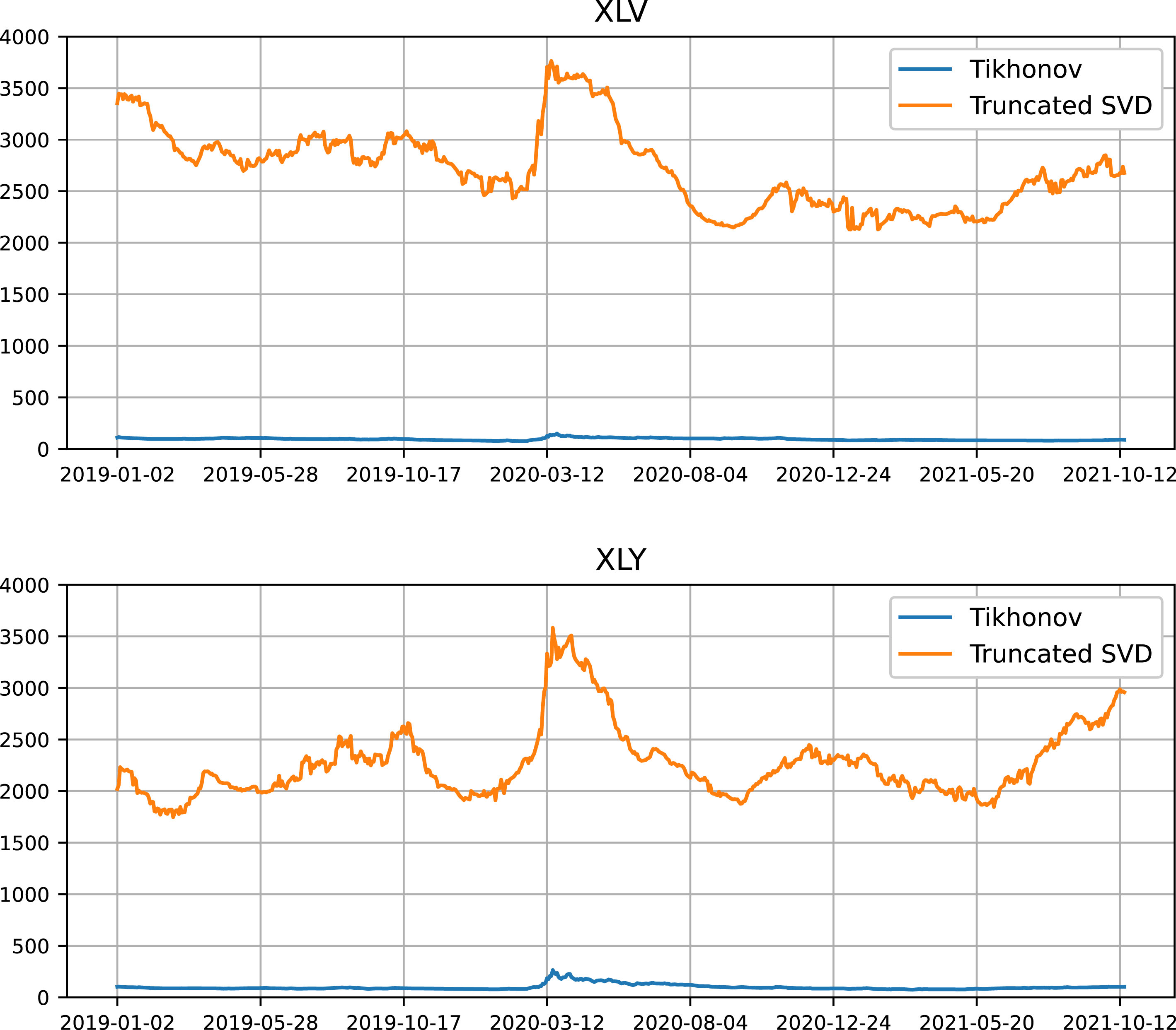
Daily condition number of minimization problems in GEDMD in the XLV and XLY universes.

Fig. 4

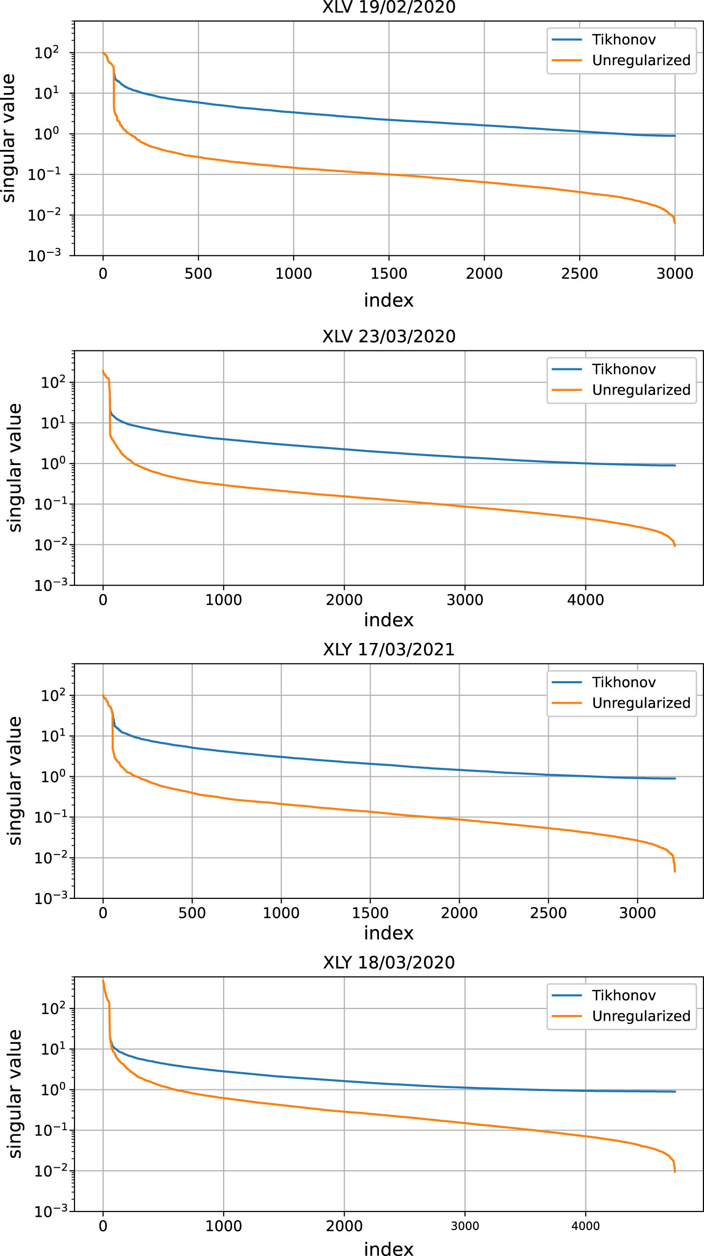
Singular values of $X_{1}^{(i)}$ in GEDMD. Top figure: XLV on the day of the lowest condition number. 2nd figure: XLV on the day of the highest condition number. 3rd figure: XLY on the day of the lowest condition number. Bottom figure: XLY on the day of the highest condition number.

To show how the distribution of the singular values is improved by the regularization, we pick the day on which the condition number of the Tikhonov method depicted in Fig. 3 is the highest, as well as the day on which the condition number is the lowest. Then, we show in Fig. 4 all the singular values of $X_{1}^{(i)}$ before and after the regularization. The singular values have been sorted in descending order. The graphs show that the singular values are bounded below by 1. In contrast, without regularization, the presence of small singular values gives rise to the increased condition numbers.

5 Conclusion

In this paper, we introduced the graph embedded dynamic mode decomposition (GEDMD) model to alleviate the potential overfitting of data in the original DMD. We proposed methods to construct graphs and to formulate the GEDMD problem. The method yields portfolios that are more diversified producing reasonable, attractive, and realistic returns. Consistent superior results are observed in different universes. To focus on the quality of the signals, we leave trading rules and portfolio optimization alone in our tests.

Footnotes

Acknowledgements

The authors would like to thank Mr. Kenny Cheung, Mr. Thomas Kwong, Mr. Ani Li, Ms. Elaine Liu, Mr. Raymond Wu, Dr. Chin-Ko Yau for their support and help in the preparation of the manuscript. Ng is supported by HKRGC GRF 12300519, 17201020 and 17300021, HKRGC CRF C1013-21GF and C7004-21GF, and Joint NSFC and RGC N-HKU769/21.

References

Bullmore, E, Sporns, O. 2009 Complex brain networks: Graph theoretical analysis of structural and functional systems, Nat Rev Neuroscience 10(3), 186–198.

Centola, D, Macy, M. 2007 Complex contagions and the weakness of long ties, Amer J Sociology 113(3), 702–734.

Ching, W, Fung, E, Ng, M. 2002 A multivariate Markov chain model for categorical data sequences and its applications in demand predictions, IMA J Manage Math 13, 187–199.

Ching, W, Fung, E, Ng, M, Ng, T. 2003 Multivariate Markov models for the correlation of multiple biological sequences, in International Workshop on Bioinformatics: PAKDD, Springer: Berlin, Seoul, Korea, pp. 23–34.

Chui, C, Mhaskar, H. 2016 Signal decomposition and analysis via extraction of frequencies, Appl Comp Har Anal 40(1), 97–136.

Cui, L, Long, W. 2016 Trading strategy based on dynamic mode decomposition: Tested in Chinese stock market, Physica A498–508.

Dicle, C, Mansour, H, Tan, D, Benosman, M, Vetro, A. 2016 Robust low rank dynamic mode decomposition for compressed domain crowd and traffic flow analysis, in IEEE International Conference on Multimedia and Expo (ICME), IEEE, Seattle, WA, USA.

Hua, J, Roy, S, McCauley, J, Gunaratne, G. 2016 Using dynamic mode decomposition to extract cyclic behavior in the stock market, Physica A 448, 172–180.

Huang, N, Shen, Z, Long, S, Wu, M, Shih, H, Zheng, Q, Yen, N, Tung, C, Liu, H. 1971 The empirical mode decomposition and the Hilbert spectrum for nonlinear and non-stationary time series analysis, Proceedings of the Royal Society of London A 454, 903–995.

10.

Jovanović, M, Schmid, P, Nichols, J. 2014 Sparsity-promoting dynamic mode decomposition, Physics of Fluids 26(2), 024103.

11.

Kuttichira, D, Gopalakrishnan, E, Menon, V, Soman, K. 2017 Stock price prediction using dynamic mode decomposition, in International Conference on Advances in Computing, Communications and Informatics (ICACCI) IEEE: New York, Udupi, India.

12.

Kutz, J, Brunton, S, Brunton, B, Proctor, J. 2000 Dynamic mode decomposition: Data-driven modeling of complex systems. SIAM:Philadelphia.

13.

Mann, J, Kutz, J. 2016 Dynamic mode decomposition for financial trading strategies, Quant Fin 16(11), 1643–1655.

14.

Prasadan, A, Nadakuditi, R. 2020 Time series source separation using dynamic mode decomposition, SIAM J Appl Dyn Syst 19(2), 1160–1199.

15.

Rowley, C, Mezić, I, Bagheri, S, Schlatter, P, Henningson, D. 2009 Spectral analysis of nonlinear flows, J Fluid Mech 641, 115–127.

16.

Salova, A, Emenheiser, J, Rupe, A, Crutchfield, J, D’Souza, R. 2019 Koopman operator and its approximations for systems with symmetries. Chaos: An Interdisciplinary Journal of Nonlinear Science 29, 093128.

17.

Schmid, P.

2010 Dynamic mode decomposition of numerical and experimental data, J Fluid Mech 656, 5–28.

18.

Schmid, P.

2022 Dynamic mode decomposition and its variants, Ann Rev of Fluid Mechanics 54, 225–254.

19.

Schmid, P, Sesterhenn, J. 2008 Dynamic mode decomposition of numerical and experimental data, in 61st Annual Meeting of the APS Division of Fluid Dynamics, American Physical Society, San Antonio, TX.

20.

Takeishi, N, Kawahara, Y, Yairi, T. 2017 Sparse nonnegative dynamic mode decomposition, in IEEE International Conference on Image Processing (ICIP), IEEE, Beijing, China.

21.

Tikhonov, A, Arsenin, V. 1977 Solution of Ill-posed Problems, Winston & Sons, Washington.

22.

Tsay, R.

2010 Analysis of Financial Time Series, 3rd edn, Wiley, New Jersey.