Combining low-volatility and mean-reversion anomalies: Better together?

Abstract

This paper contributes to the existing stock market anomaly literature by being the first to analyze the benefits of combining two distinct anomalies; specifically, the low-volatility and mean-reversion anomalies. Our results show that on a long-only basis, these two time-varying anomalies could be combined into a double-sort investment strategy that includes some desirable characteristics from each of them, thereby making the portfolio return accumulation more stable over time. As the added-value of low-volatility investing stems mostly from the risk-reduction side, while contrarian stocks are generally highly volatile with remarkable upside potential, the use of the double-sort portfolio-formation in which the contrarian stocks are picked from the sub-set of below-median volatility stocks can shorten the below-market performance periods that have occasionally materialized for plain low-volatility or plain contrarian investors.

Abstract

JEL classification: G11

Keywords

Volatility contrarian mean reversion anomaly portfolio performance equity investing

1. Introduction

We contribute to the existing anomaly literature by being the first to analyze the benefits of combining two stock market anomalies that are distinct from each other, namely low-volatility and mean-reversion anomalies.¹ The motivation for combining these two anomalies into a single portfolio-formation criterion stems from the following facts: Although long-term evidence for the low-volatility anomaly is well-documented, intermediate-term periods during which high-volatility stocks outperform low-volatility stocks in terms of absolute returns are not rare.² In addition, the added-value of low-volatility investing has mostly stemmed from risk-reduction side, rather than from return-enhancement side. For example, Kenneth French’s comprehensive U.S. data set (available at http://mba.tuck.dartmouth.edu/pages/faculty/ken.french/data_library.html) shows that although the volatilities of the decile portfolios formed on 60-day variance over the 57 1/2 -year period from 1963:07 to 2020:12 are monotonically increasing from the lowest-decile to the highest-decile portfolios, their returns do not show such monotonicity: Their return pattern is rather inversely U-shaped, with highest decile return being reported for the fourth-highest-volatility decile with a remarkable value-weighted (equally-weighted) return difference of 2.14% (3.38%) p.a. to the low-volatility decile portfolio that is the third-lowest (second-lowest) in the value-weighted (equally-weighted) decile-return ranking.

By contrast, among the decile portfolios formed on the 48-month contrarian indicator lagged by 12 months, the bottom-decile portfolio consisting of prior-loser stocks is the one with clearly the highest return on both value- and equally-weighted basis. Particularly, an equally-weighted bottom-decile contrarian raw return is spectacular, being at 18.07% p.a. way higher than the corresponding returns reported for the low-volatility decile portfolios. However, there is an obvious return-risk trade-off, as the bottom-decile portfolios are the most volatile among the contrarian decile portfolios. Because the low-volatility anomaly seems to stem from risk reduction, whereas the mean-reversion anomaly is driven by high returns coupled with high volatility, it is worthwhile to study whether these two strongly time-varying anomalies³ could be combined into a single investment strategy that could include some desirable characteristics from both of these investment strategies and make the portfolio return accumulation more stable over time. Further motivation for combining volatility and mean-reversion in portfolio formation is given by the fact that the correlation of long-short factors formed on the basis of volatility and contrarian indicators is significantly negative over the period from 1963:07 to 2020:12, over which both factors are available in French’s data library.

To the best of our knowledge, the benefits of combining volatility and contrarian indicators have not been discussed in earlier literature on equity investment strategies. Volatility and mean-reversion anomalies are also particularly interesting in the respect that their existence violates even the weak-form market efficiency (Fama 1970), according to which all historical information related to prices, returns, and trading volumes etc. should be useless for generating abnormal risk-adjusted returns. Hence, the existence of these anomalies would imply that abnormal returns could be earned by employing simple trading algorithms without paying any attention to firm fundamentals. Interestingly, earlier literature has provided some evidence for interlinkage between value and low-volatility stocks (e.g., see Scherer, 2011; Walkshäusl, 2013; Chow et al., 2014; Goldberg, Lesheem, and Geddes, 2014), as well as between value and contrarian stocks (e.g., see Lakonishok, Shleifer, and Vishny, 1994; Asness, Moskowitz, and Pedersen, 2013). In light of these findings, it is intriguing to examine how strong value-like characteristics the double-sort portfolios formed on volatility and contrarian indicators could have without using any financial statement data in portfolio formation. We analyze this on the basis of Fama-French-Carhart 6-factor model (Carhart, 1997; Fama and French, 2018), which also reveals the comparable style exposures to firm size, operating profitability, asset growth, and price momentum. For comparability purposes, we also report the corresponding factor exposures for single-sorted volatility and contrarian portfolios.

Further motivation for focusing on low-volatility and mean-reversion anomalies is given by the fact that in the three top-tier finance journals, these two anomalies have very seldom been discussed in 2000 s, although at least in terms of raw returns, the post-millennium period has been favorable for both of these anomalies. In our opinion, the main reason for the scarcity of recent literature on mean-reversion anomaly is in its strong time-variability: As documented by Zaremba, Kizys, and Raza (2020), the mean-reversion effect may disappear for periods as long as several decades. In addition, it is also well known that contrarian profits are driven by small-caps (e.g., see Hou, Xue, and Zhang, 2020), being therefore prone to high trading costs, unlike low-volatility strategies, which are relatively cheap to implement. Although literature on low-volatility anomaly is much more numerous particularly in more pragmatically-oriented journals⁴, such papers, in which the joint-effect of volatility and contrarian indicators is examined, are non-existent. For these reasons, our paper focuses on filling this research gap. We also contribute to the existing literature by revealing some interesting differences in time-variability of return-generation patterns between low-volatility and contrarian stocks, thereby offering a partial explanation for potential benefits of combining these two anomalies.

Several studies have shown that anomalies tend to suffer from post-publication decline, according to which abnormal profits from any investment strategy attenuate soon after academic publication of an underlying anomaly (e.g. see McLean and Pontiff, 2016; Linnainmaa and Roberts, 2018). Particularly, the post-millennium period has proven to be challenging for almost all conventional stock market anomalies (Arnott et al., 2019). Based on the related literature it seems that the reason for attenuation or disappearance of anomalies has at least partially lain in the fact that the post-millennium period has included many sub-periods during which short legs of many anomalous long-short portfolios have generated much higher returns than the corresponding long legs (e.g., see Daniel and Moskowitz, 2016; Blitz, 2021). Therefore, our main focus is on long-only portfolio performance net of transaction costs, although we first report the gross performance statistics throughout all the quantile portfolios, as well as for the long-short portfolios. The long-only focus is also justified as it is far less frequently examined than the long-short approach, although most equity investors operate only in the long-only universe. From the viewpoint of practical implementability, the transaction costs are much higher for short than long positions: E.g., Drechsler and Drechsler (2016) found that shorting fees are more than three times higher than normal for the short leg of volatility-related portfolios. Beneish, Lee, and Nichols (2015) show that the stocks with the highest attractiveness among short sellers are often least available to borrow. Short selling also entails additional risks, such as “short squeeze” scenarios (in which investors are unable to close their short positions), thereby increasing the loan fees of small-cap stocks, particularly (see, e.g., Cohen, Diether, and Malloy, 2007; Blitz, Baltussen, and van Vliet, 2020). Occasionally, legal impediments to short selling may also exist (see, e.g., D’Avolio, 2002; Barber and Odean, 2008; Beneish et al., 2015; Patton and Weller, 2020).

Our main findings can be summarized as follows: By using the double-sort portfolio-formation criterion in which the contrarian stocks are picked from the sub-set of below-median volatility stocks, contrarian and low-volatility anomalies can be combined into an investment strategy that includes some desirable characteristics from each of them. The use of the double-sort criterion can make the portfolio return accumulation more stable over time and shorten the durations of the below-market performance periods that have occasionally materialized for plain low-volatility or plain contrarian investors.

The structure of the paper is as follows. Section 2 describes the data, while section 3 explains the methodology employed. Section 4 introduces the empirical results, followed by the conclusions in Section 5.

2. Data

The sample data consist of all firms without any industry restrictions on the NYSE, AMEX, and Nasdaq with reliable data from the Center for Research in Security Prices (CRSP). Because the CRSP return data to which we have access starts from 1962:07, the first time-point at which 60-month return history is available for contrarian portfolio-formation is 1967:07. However, because of well-documented seasonality characteristics of contrarian returns, we shift the starting point of the sample period forward by 6 months to January 1968.⁵ For sake of comparability, we also use the same date as the starting point for forming volatility portfolios. The full-length investment period extends to December 2020, including 53 calendar years. Before any filtering procedures, the sample is composed of 23,283 firms with ordinary common equity on CRSP (share code 10 or 11). Consistent with Lee and Ogden (2015), Stambaugh and Yuan (2017), and Chen et al. (2021), among many others, we exclude the firms whose stock prices are below $5 on a portfolio-formation date. The continuous monthly-return history over the preceding selection period is required for the stocks included in the investable universe at each checkpoint. Depending on updating frequency of portfolios, the number of firms that at some stage of the 53-year sample period have belonged to the investable universe ranges from 19,423 (in the case of annual updating frequency) to 21,028 (in the case of monthly updating frequency). In the case of semiannual updating frequency, the corresponding number is 20,243. Adjustments of returns for dividends, splits and capitalization issues are made appropriately. To avoid survivorship bias, CRSP delisting returns are incorporated according to Beaver, McNichols, and Price (2007), with the exception that we updated delisting return estimates for firms with missing delisting returns on CRSP for each stock exchange based on the available and traceable delisting returns over the period 1968:01–2020:12.

3. Methodology

3.1. Portfolio formation principles

First, we form single-sorted decile portfolios based on volatility and contrarian indicators. In line with Blitz and van Vliet (2007, 2018), we use the standard deviation calculated over 36 monthly returns as a volatility indicator.⁶ Following Fama and French (1996), Jacobs (2015), and Zaremba et al. (2020), among others, we use 48-month historical return, skipping the most recent year, as the contrarian indicator (henceforth denoted as 60M-12M). Because the performance of trading portfolios is also dependent on trading frequency, the impact of holding period length on the results is also examined by updating the portfolios on monthly, semiannual and annual bases, in accordance with Hou et al. (2020).

Besides single-sorted portfolios, we form double-sorted quantile portfolios by using 2×5 sequential sorts, dividing first the investable sample at each portfolio-(re)formation point into halves based on volatility and further, into quintiles within these halves based on contrarian indicators. Because the near-term future volatility is significantly higher for the top-half portfolios formed on historical volatility than for the corresponding bottom-half portfolios, whereas the return difference between the bottom- and top-half contrarian portfolios is insignificant, we report the double-sort results only for the portfolios, for which the volatility is employed as the first-stage criterion, followed by the second-stage sorts based on the contrarian indicator.

Over all portfolio-formation criteria, we rebalance the weights of constituent stocks in each quantile portfolio to 1/N at each portfolio-formation date and calculate the monthly portfolio returns by taking account of the weight changes stemming from the return differences of constituent stocks within the holding periods, in line with Liu and Strong (2008).⁷ The employed weighting system was chosen instead of value-weighting because the latter weighting system strongly deteriorates the mean-reversion anomaly.⁸ Moreover, for some sub-periods the value-weighted portfolios are dominated by just few megacaps, which make the portfolios poorly diversified in such circumstances (e.g., see also Blitz, Hanauer, and Vidojevic, 2020). For these reasons, hardly any portfolio manager would weight the constituent stocks based strictly on their market caps when deciding on portfolio allocation. Therefore, from the viewpoint of practical implementability of trading strategies, which is the focus of this study, our approach is more realistic and simpler.⁹

Of course, there are also downsides stemming from re-balancing the portfolio weights at each portfolio-reformation point. Because small-caps and particularly microcaps are more expensive to trade than large-caps, it is evident that average trading-cost percentages are higher for equally-weighted than for value-weighted portfolios.¹⁰ It is possible that small- and microcap trading costs are higher to the extent that all the anomalous paper profits are absorbed by them. Therefore, it is particularly important to take account of trading costs in a realistic manner when the implementation of a trading strategy requires transactions in the low-end market-cap universe of stocks, as in the case of contrarian strategies.

3.2. Estimation of trading costs

We estimate one-way transaction costs as the sum of historical effective spreads and trading commissions. For each stock at each portfolio-formation point, the effective half-spread component is estimated on the basis of daily high, low and close prices, in line with Abdi and Ranaldo (2017)¹¹ as follows:

h a l f - s p r e a d = \sqrt{E [(c_{t} - η_{t}) (c_{t} - η_{t + 1})]}

(1)

in which c is the daily close log-price and η is the daily mid-range (i.e., the average of daily high and low log-prices). The brokerage commissions are approximated on the basis of commission percentages provided by Jones (2002), Goldstein et al. (2009), and Di Maggio, Egan, and Franzoni (2022). The approximated range of one-way commissions is from 0.12% to 0.90%, peaking in the turn of the years 1973 and 1974 (during OPEC oil crisis). As a result, we get individual one-way trading cost estimates for every stock in the sample for all portfolio-formation points.¹² In the beginning of the holding period, we reduce the stock-specific trading cost percentage (TC%) from the initial investment in that particular stock. Then we calculate the return accumulation at the portfolio level up to the following portfolio-reformation time-point, at which point the trading costs are calculated so that if a stock A continues as a constituent of the portfolio over the portfolio-reformation point, the trading costs stemming from rebalancing are determined as follows:

| \frac{A_{t + n}}{P_{t + n}} - \frac{1}{N} | \times T C %_{t + n}

, where A_t+n is the total value of A stocks in the portfolio as end of the n-month investment period, P_t+n is the total value of the whole portfolio at the same time-point, and N is the number of the stock series in the rebalanced portfolio.

The net value for the stock A in the end of n-month holding period is calculated by multiplying the product of n monthly gross returns (expressed as 1 + r_p.m.) by the product of [(1 - TC % _t)/1] and $[1 - (| \frac{A_{t + n}}{P_{t + n}} - \frac{1}{N} | \times T C %_{t + n})]$ . The first term in the latter product inflates the cumulative gross return by the amount of initial purchasing costs, whereas the second takes account of the dilution stemming from the rebalancing costs at the end of n-month holding period. The same procedure is repeated for all such stocks which continue as constituents of the portfolio over the portfolio-reformation point.

If a stock B drops out of the re-formatted portfolio, the return decrease stemming from total sales of such stock holdings is as follows:

\frac{B_{t + n}}{P_{t + n}} \times T C %_{t + n}

(2)

A similar calculation is repeated for all such dropped-out stocks. For longer than monthly holding periods, the portfolio net returns for the subsequent month (i.e., the first month after re-balancing) are given by multiplying the average of new entrants’ trading cost percentages by the number of new entrants, dividing the resulting product by the total number of stock series in the re-formatted portfolio (including those stocks that were already in the portfolio before the reformation), and finally, subtracting the resulting percentage from the corresponding monthly gross return. In the case of monthly updating, the purchasing costs caused by the inclusion of new entrants, rebalancing costs of the remaining constituent stocks, as well as the selling costs of dropped-out stocks must all be subtracted within the same month.

At the end of the 53-year sample period, the trading cost percentage stemming from cashing the portfolios is calculated as the weighted trading cost average of all the stocks that are then in the portfolio, by using the closing stock-specific portfolio weights in the calculation of the weighted average. Hence, we assume that all the constituent stocks are sold at the end of the sample period.

Interestingly, Novy-Marx and Velikov (2016, 2019) show that the return dilution caused by trading costs can be alleviated by means of cost-mitigation techniques. In their comparisons of three cost-mitigation techniques, superiority over two others¹³ was shown by the so-called “buy/hold spread” or “banding” technique, which involves employing a more stringent threshold for opening new positions than for retaining already-existing positions. We implement this technique for our low-volatility and contrarian portfolios, as well as for the bottom-quantile double-sort combination portfolio, by holding the constituent stocks once they have entered the bottom-decile threshold until they rise above the bottom-30%. For the sake of comparability, we also report post-cost performance statistics for the corresponding portfolios formed without any cost-mitigation actions.

3.3. Performance metrics and statistical tests for portfolio comparisons

The performance of quantile portfolios is evaluated based on three different performance metrics; geometric average net return, the Sharpe ratio (Sharpe, 1966), and the Fama-French-Carhart 6-factor alpha (Carhart, 1997; Fama and French, 2018). We use the equal-weighted sample-specific portfolios consisting of all the investable stocks as the benchmark portfolio for sake of robustness.¹⁴ The 6-factor regression model, from which the alphas are derived, is as follows (all the factor spread returns were downloaded from French’s data library):

\begin{aligned} r_{i t} - r_{f t} & = α_{i} + b_{i} (r_{m t} - r_{f t}) + s_{i} S M B_{t} + h_{i} H M L_{t} \\ + c_{i} C M A_{t} + r_{i} R M W_{t} + m_{i} U M D_{t} + ε_{i t} \end{aligned}

(3)

where r_it= the return of a portfolio, r_ft= the risk-free rate of return, α _i= the 6-factor alpha (the abnormal return over and above what might be expected based on the 6-factor model employed), r_mt= the sample-specific stock market return, SMB_t= the return of the size factor (i.e, the return difference between small- and large-cap portfolios), HML_t= the return of the book-to-market (B/P) factor (i.e, the return difference between high- and low-B/P portfolios), CMA_t= the return difference between the portfolios of conservatively and aggressively investing firms, RMW_t= the return return difference between robust and weak operating profitability firms, UMD_t= the return of the momentum factor (i.e, the return difference between winner and loser stock portfolios), b_i, s_i, h_i, c_i, r_i and m_i are factor sensitivities to stock market, SMB, HML, CMA, RMW, and UMD factors, respectively, and ɛ_it= the residual term.

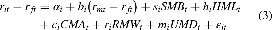
The statistical significances of the differences between comparable pairs of the Sharpe ratios are given by the p-values of the Ledoit-Wolf (2008) test, which is based on the circular block bootstrap method, taking also account of skewness and kurtosis of return distributions being compared, as well as the impact of autocorrelation.¹⁵ The significance of 6-factor alphas is based on their t-statistic, which is closely related to a multifactor version of the Treynor-Black (1973) appraisal ratio. Throughout the regressions, we use the Newey-West (1987) HAC-adjusted standard errors to minimize the estimation biases caused by autocorrelation and heteroscedasticity.

4. Results

4.1. Results for the full sample period

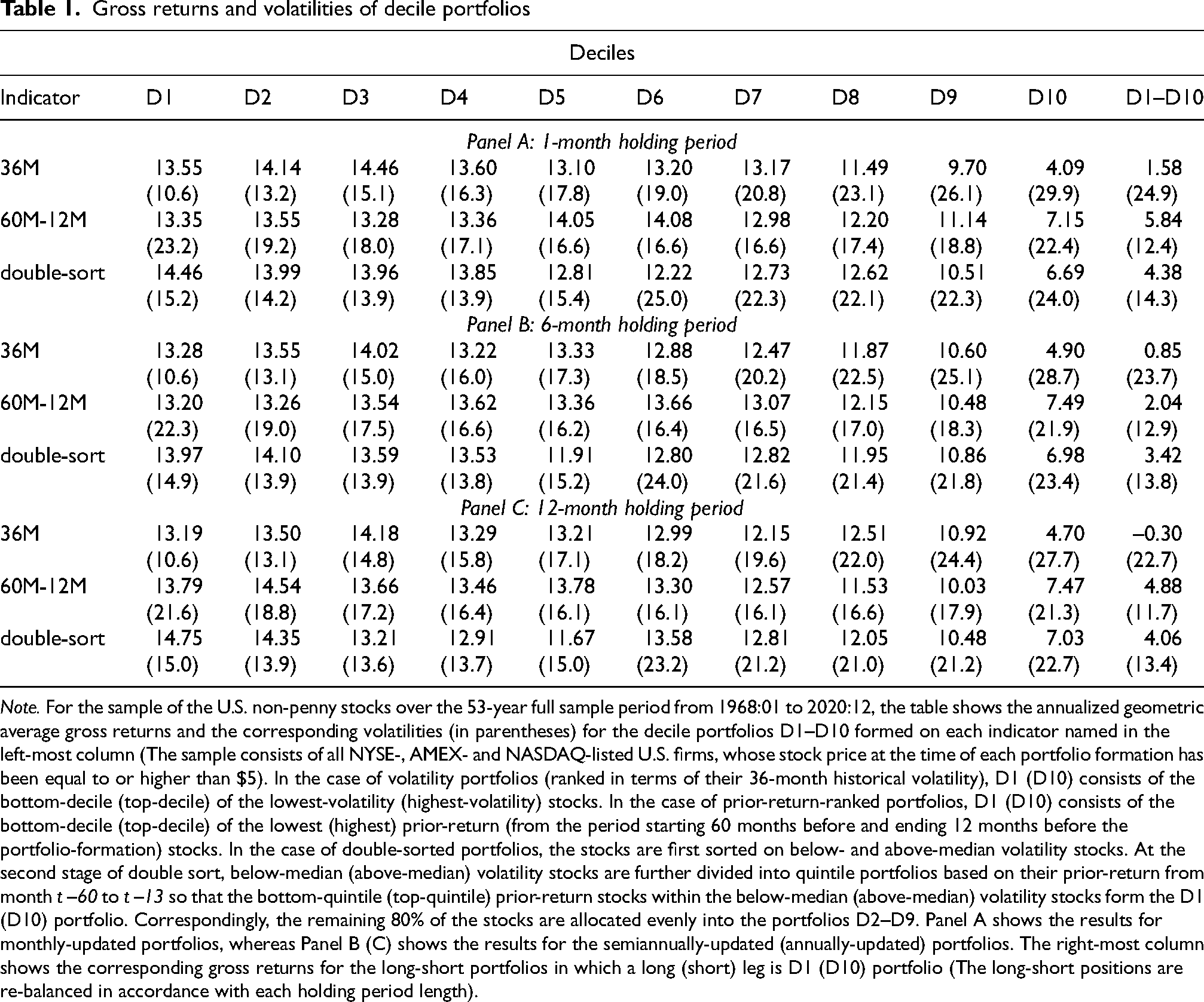
To get a preliminary view on discriminatory power of the examined portfolio-formation criteria, Table 1 shows the annualized geometric average before-transaction-cost returns and volatilities for decile portfolios formed on volatility and contrarian indicators, as well as the double-sorted quantile portfolios formed on 2×5 sequential sorts. In the case of volatility-sorted portfolios, D1 (D10) consists of the bottom-10% (top-10%) of the lowest-volatility (highest-volatility) stocks, whereas in the case of the portfolios formed on contrarian indicators, D1 (D10) consists of the bottom-decile (top-decile) of the stocks sorted on their prior-return from the period starting 60 months before and ending 12 months before the portfolio-formation. Correspondingly, the remaining 80% of the stocks are allocated evenly into the portfolios D2–D9. In the case of double-sorted portfolios, the stocks are first sorted on below- and above-median volatility stocks. At the second stage of double sort, below-median (above-median) volatility stocks are further divided into quintile portfolios based on their prior-return from month t –60 to t –13 so that the bottom-quintile (top-quintile) prior-return stocks within the below-median (above-median) volatility stocks form the D1 (D10) portfolio. Correspondingly, the double-sorted D2–D5 (D6–D9) portfolios are below-median (above-median) volatility stocks, whose prior-returns monotonically increase from D2 (D6) towards D5 (D9).

Panel A shows the results for the monthly-updated portfolios. In terms of gross returns, D1 portfolios formed on volatility and contrarian indicators are not the highest-yield decile portfolios among each decile group, whereas among double-sorted below-median volatility stocks the gross returns are monotonically decreasing from D1 to D5, thereby indicating the mean-reversion tendency within the low-volatility stocks. Interestingly, the lowest gross return among the double-sorted quantiles from D1 to D5 is higher than the greatest gross return among the comparable quantiles from D6 to D10, while at the same time, the highest volatility among the first group of double-sort portfolios is considerably lower than the lowest volatility among the latter group. These findings give further justification to test the efficacy of such combination criteria, where the first-stage sort is based on volatility, followed by the second-stage mean-reversion sorts.

Although the condition of monotonically decreasing decile returns is not met for both univariate criterion, gross performance statistics still reveal some interesting insights: For the deciles sorted on their historical volatility, the portfolio volatilities are monotonically increasing in a very prominent way, as the annualized standard deviation almost triples when moving from D1 to D10. Hence, volatility characteristics seem to persist surprisingly well at portfolio level, as is also documented in previous literature (see, e.g., Clarke et al. 2006). By contrast, the monotonicity condition is not met with the volatility pattern of the deciles formed on contrarian indicator, which is inversely U-shaped, similarly to earlier results of Fama and French (1996). In addition, when the top-bottom decile return spreads are calculated on the basis of annualized geometric average return differences between the bottom and top deciles, as done in the rightmost column of Table 1, the spreads are surprisingly low, being 5.84% p.a. at their highest among the monthly-updated contrarian portfolios. This shows that the simple way employed commonly in related literature to calculate the spread by subtracting the average short-leg return from the average long-leg return is often highly misleading. Among the examined investment strategies, it would be partially misleading for the monthly-updated long-short volatility portfolio, as the top-bottom spread (or hypothetical long-short return) calculated in the above-described too simple way is 9.46% p.a. (4.76% p.a.) in terms of geometric (arithmetic) average returns, whereas the annualized geometric average top-bottom spread calculated on the basis of monthly return differences between long and short legs, indicating the true average top-bottom gross return earned over the full sample period, is only 1.58% p.a. In light of this fact, and coupled with the fact that the annualized volatility of the top-bottom decile-spread is simultaneously as high as 24.9%, it is obvious that long-short investing relying on volatility-sorted extreme deciles and monthly updating of long/short positions would have been disastrous even in the world without any trading costs.

Table 1.
Gross returns and volatilities of decile portfolios

Deciles

Indicator D1 D2 D3 D4 D5 D6 D7 D8 D9 D10 D1–D10

Panel A: 1-month holding period

36M 13.55 14.14 14.46 13.60 13.10 13.20 13.17 11.49 9.70 4.09 1.58

(10.6) (13.2) (15.1) (16.3) (17.8) (19.0) (20.8) (23.1) (26.1) (29.9) (24.9)

60M-12M 13.35 13.55 13.28 13.36 14.05 14.08 12.98 12.20 11.14 7.15 5.84

(23.2) (19.2) (18.0) (17.1) (16.6) (16.6) (16.6) (17.4) (18.8) (22.4) (12.4)

double-sort 14.46 13.99 13.96 13.85 12.81 12.22 12.73 12.62 10.51 6.69 4.38

(15.2) (14.2) (13.9) (13.9) (15.4) (25.0) (22.3) (22.1) (22.3) (24.0) (14.3)

Panel B: 6-month holding period

36M 13.28 13.55 14.02 13.22 13.33 12.88 12.47 11.87 10.60 4.90 0.85

(10.6) (13.1) (15.0) (16.0) (17.3) (18.5) (20.2) (22.5) (25.1) (28.7) (23.7)

60M-12M 13.20 13.26 13.54 13.62 13.36 13.66 13.07 12.15 10.48 7.49 2.04

(22.3) (19.0) (17.5) (16.6) (16.2) (16.4) (16.5) (17.0) (18.3) (21.9) (12.9)

double-sort 13.97 14.10 13.59 13.53 11.91 12.80 12.82 11.95 10.86 6.98 3.42

(14.9) (13.9) (13.9) (13.8) (15.2) (24.0) (21.6) (21.4) (21.8) (23.4) (13.8)

Panel C: 12-month holding period

36M 13.19 13.50 14.18 13.29 13.21 12.99 12.15 12.51 10.92 4.70 –0.30

(10.6) (13.1) (14.8) (15.8) (17.1) (18.2) (19.6) (22.0) (24.4) (27.7) (22.7)

60M-12M 13.79 14.54 13.66 13.46 13.78 13.30 12.57 11.53 10.03 7.47 4.88

(21.6) (18.8) (17.2) (16.4) (16.1) (16.1) (16.1) (16.6) (17.9) (21.3) (11.7)

double-sort 14.75 14.35 13.21 12.91 11.67 13.58 12.81 12.05 10.48 7.03 4.06

(15.0) (13.9) (13.6) (13.7) (15.0) (23.2) (21.2) (21.0) (21.2) (22.7) (13.4)

Deciles
Panel A: 1-month holding period
36M	13.55	14.14	14.46	13.60	13.10	13.20	13.17	11.49	9.70	4.09	1.58
	(10.6)	(13.2)	(15.1)	(16.3)	(17.8)	(19.0)	(20.8)	(23.1)	(26.1)	(29.9)	(24.9)
60M-12M	13.35	13.55	13.28	13.36	14.05	14.08	12.98	12.20	11.14	7.15	5.84
	(23.2)	(19.2)	(18.0)	(17.1)	(16.6)	(16.6)	(16.6)	(17.4)	(18.8)	(22.4)	(12.4)
double-sort	14.46	13.99	13.96	13.85	12.81	12.22	12.73	12.62	10.51	6.69	4.38
	(15.2)	(14.2)	(13.9)	(13.9)	(15.4)	(25.0)	(22.3)	(22.1)	(22.3)	(24.0)	(14.3)
Panel B: 6-month holding period
36M	13.28	13.55	14.02	13.22	13.33	12.88	12.47	11.87	10.60	4.90	0.85
	(10.6)	(13.1)	(15.0)	(16.0)	(17.3)	(18.5)	(20.2)	(22.5)	(25.1)	(28.7)	(23.7)
60M-12M	13.20	13.26	13.54	13.62	13.36	13.66	13.07	12.15	10.48	7.49	2.04
	(22.3)	(19.0)	(17.5)	(16.6)	(16.2)	(16.4)	(16.5)	(17.0)	(18.3)	(21.9)	(12.9)
double-sort	13.97	14.10	13.59	13.53	11.91	12.80	12.82	11.95	10.86	6.98	3.42
	(14.9)	(13.9)	(13.9)	(13.8)	(15.2)	(24.0)	(21.6)	(21.4)	(21.8)	(23.4)	(13.8)
Panel C: 12-month holding period
36M	13.19	13.50	14.18	13.29	13.21	12.99	12.15	12.51	10.92	4.70	–0.30
	(10.6)	(13.1)	(14.8)	(15.8)	(17.1)	(18.2)	(19.6)	(22.0)	(24.4)	(27.7)	(22.7)
60M-12M	13.79	14.54	13.66	13.46	13.78	13.30	12.57	11.53	10.03	7.47	4.88
	(21.6)	(18.8)	(17.2)	(16.4)	(16.1)	(16.1)	(16.1)	(16.6)	(17.9)	(21.3)	(11.7)
double-sort	14.75	14.35	13.21	12.91	11.67	13.58	12.81	12.05	10.48	7.03	4.06
	(15.0)	(13.9)	(13.6)	(13.7)	(15.0)	(23.2)	(21.2)	(21.0)	(21.2)	(22.7)	(13.4)

Note. For the sample of the U.S. non-penny stocks over the 53-year full sample period from 1968:01 to 2020:12, the table shows the annualized geometric average gross returns and the corresponding volatilities (in parentheses) for the decile portfolios D1–D10 formed on each indicator named in the left-most column (The sample consists of all NYSE-, AMEX- and NASDAQ-listed U.S. firms, whose stock price at the time of each portfolio formation has been equal to or higher than $5). In the case of volatility portfolios (ranked in terms of their 36-month historical volatility), D1 (D10) consists of the bottom-decile (top-decile) of the lowest-volatility (highest-volatility) stocks. In the case of prior-return-ranked portfolios, D1 (D10) consists of the bottom-decile (top-decile) of the lowest (highest) prior-return (from the period starting 60 months before and ending 12 months before the portfolio-formation) stocks. In the case of double-sorted portfolios, the stocks are first sorted on below- and above-median volatility stocks. At the second stage of double sort, below-median (above-median) volatility stocks are further divided into quintile portfolios based on their prior-return from month t –60 to t –13 so that the bottom-quintile (top-quintile) prior-return stocks within the below-median (above-median) volatility stocks form the D1 (D10) portfolio. Correspondingly, the remaining 80% of the stocks are allocated evenly into the portfolios D2–D9. Panel A shows the results for monthly-updated portfolios, whereas Panel B (C) shows the results for the semiannually-updated (annually-updated) portfolios. The right-most column shows the corresponding gross returns for the long-short portfolios in which a long (short) leg is D1 (D10) portfolio (The long-short positions are re-balanced in accordance with each holding period length).

When extending the holding-period length to six months (Panel B), the results remain essentially the same with the following exceptions: In comparison with monthly-updated portfolios, the bottom-quantile gross returns as well as the corresponding top-bottom spreads are slightly lower. In addition, the discriminatory power of volatility in double-sorts is not as high as it is among the monthly-updated portfolios, although the highest volatility among the portfolios from D1 to D5 is still considerably lower than the lowest volatility among the portfolios from D6 to D10. Of course, the inclusion of transaction costs affects the relative performance of the portfolios updated with different frequencies and therefore, we keep the pre-cost performance comparison brief.

The further extension of the holding-period length to twelve months (Panel C) reveals some additional, interesting findings: First, the bottom-quantile returns of the portfolios formed on contrarian indicator and on double-sort criterion are higher than for shorter holding-period lengths. The bottom-decile double-sort portfolio generates the highest gross return reported across all the trading portfolios included in Table 1. Moreover, it does that with a reasonable volatility (of 15.0% p.a.), which is three percentage points lower than the volatility of the comparable benchmark portfolio. Generally, the double-sort criterion employed seems to have a desirable characteristic of considerably reducing a high volatility of contrarian portfolios, while simultaneously offering a higher return potential than low-volatility portfolios. To find out to what extent this performance-enhancement potential can be materialized in the real world, we will next include the transaction costs in performance comparisons and analyze the benefits of cost-mitigation for the employed trading strategies.

As is already justified in Introduction, as well as based on the conclusions drawn from gross return statistics discussed above, we will henceforth focus on performance comparisons of long-only bottom-quantile portfolios. Table 2 shows the post-cost performance statistics for the bottom-quantile portfolios formed on the two single-sort criteria, as well as on the previously-introduced double-sort criterion. The right side of Table 2, showing the post-cost performance statistics for the bottom-decile portfolios managed without any cost-mitigation actions, reveals some interesting impacts of trading cost inclusion: First, the performance statistics of bottom-decile low-volatility portfolios are surprisingly similar across the holding periods: Particularly, their net returns and Sharpe ratios are almost identical, thereby showing that their pre-cost performance differences are smoothened out by lower trading costs of the portfolios updated less frequently. The turnover statistics of these volatility-based decile portfolios reveal that the average annual turnover rate for a corresponding monthly-updated portfolios is 68.9%, resulting in annual return reduction of 64 basis points caused by trading costs. By contrast, for the annually-updated low-volatility decile portfolio, the return dilution caused by transaction costs is only 26 basis points, which is in line with turnover rate of 26.7%.

Table 2.

Performance of the bottom-quantile portfolios with and without cost mitigation

	With cost-mitigation strategy					Without cost-mitigation strategy
Indicator	NR (%)	SR	p value (%)	α (%)	TO (%)	NR (%)	SR	p value (%)	α (%)	TO (%)
Panel A: 1-month holding period
36M	13.63	0.783	(0.0)	2.42^*	13.6	12.91	0.775	(0.0)	2.38^*	68.9
60M-12M	13.02	0.441	(65.4)	2.21	40.0	10.94	0.372	(28.3)	–1.59	236.6
double-sort	13.90	0.656	(0.0)	1.68^*	50.4	12.58	0.562	(0.7)	0.07	200.0
Panel B: 6-month holding period
36M	13.26	0.761	(0.0)	2.15^*	9.9	12.94	0.778	(0.0)	2.36^*	35.9
60M-12M	13.73	0.475	(31.1)	2.75^**	27.4	12.25	0.431	(94.0)	–0.45	92.6
double-sort	14.14	0.673	(0.0)	1.78^*	30.4	13.22	0.607	(0.1)	0.63	78.3
Panel C: 12-month holding period
36M	13.06	0.749	(0.4)	1.80^*	8.4	12.93	0.777	(0.9)	2.16^**	26.7
60M-12M	14.78	0.524	(2.5)	3.10^**	23.9	13.13	0.475	(38.8)	–0.07	64.0
double-sort	14.58	0.696	(0.0)	1.96^*	24.1	14.23	0.666	(0.4)	1.21^***	53.1

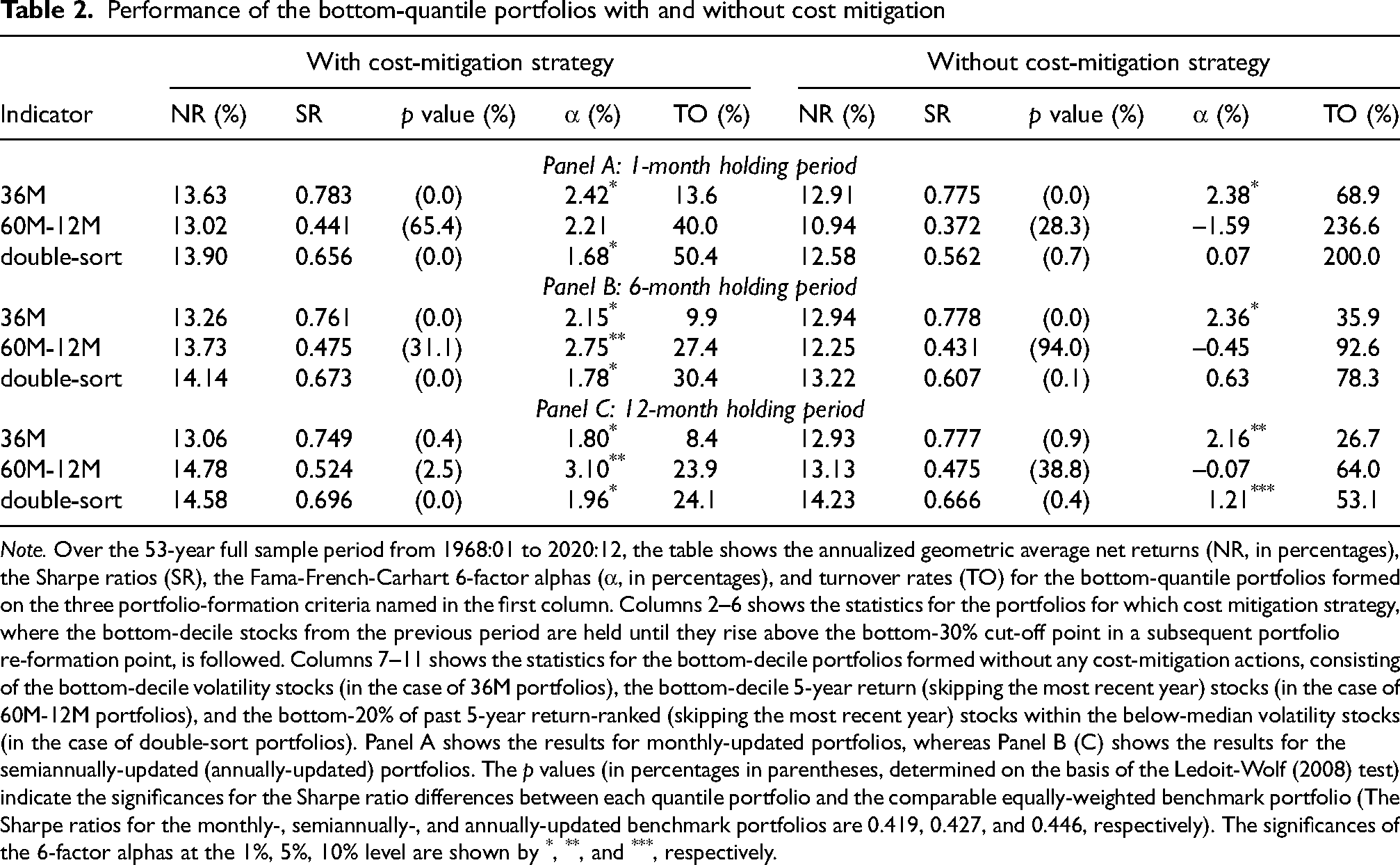
Note. Over the 53-year full sample period from 1968:01 to 2020:12, the table shows the annualized geometric average net returns (NR, in percentages), the Sharpe ratios (SR), the Fama-French-Carhart 6-factor alphas (α, in percentages), and turnover rates (TO) for the bottom-quantile portfolios formed on the three portfolio-formation criteria named in the first column. Columns 2–6 shows the statistics for the portfolios for which cost mitigation strategy, where the bottom-decile stocks from the previous period are held until they rise above the bottom-30% cut-off point in a subsequent portfolio re-formation point, is followed. Columns 7–11 shows the statistics for the bottom-decile portfolios formed without any cost-mitigation actions, consisting of the bottom-decile volatility stocks (in the case of 36M portfolios), the bottom-decile 5-year return (skipping the most recent year) stocks (in the case of 60M-12M portfolios), and the bottom-20% of past 5-year return-ranked (skipping the most recent year) stocks within the below-median volatility stocks (in the case of double-sort portfolios). Panel A shows the results for monthly-updated portfolios, whereas Panel B (C) shows the results for the semiannually-updated (annually-updated) portfolios. The p values (in percentages in parentheses, determined on the basis of the Ledoit-Wolf (2008) test) indicate the significances for the Sharpe ratio differences between each quantile portfolio and the comparable equally-weighted benchmark portfolio (The Sharpe ratios for the monthly-, semiannually-, and annually-updated benchmark portfolios are 0.419, 0.427, and 0.446, respectively). The significances of the 6-factor alphas at the 1%, 5%, 10% level are shown by ^*, ^**, and ^***, respectively.

The right-side statistics reported in Table 2 also show that for the simple contrarian portfolios, post-cost performance statistics improve towards the longer holding period lengths. However, without any cost-mitigation actions, the contrarian top-decile portfolios are not able to significantly outperform their benchmark portfolios in terms of either Sharpe ratios or 6-factor alphas. In relative terms, the performance statistics of the non-cost-mitigated double-sort portfolios are somewhat ambiguous, as in terms of the Sharpe ratios, all three have significantly outperformed their benchmark portfolio, whereas their 6-factor alphas indicate that none of them has generated significant (at the 5% level) abnormal returns over and above the joint explanatory effect of the related six factor spreads. It is also noteworthy that both contrarian and double-sorted portfolios have remarkably higher turnover rates than the corresponding low-volatility portfolios. This difference is particularly prominent for the 1-month holding-period length.

The left side of Table 2 shows that the net returns of the cost-mitigated bottom-quantile portfolios are always higher than those of the corresponding non-cost-mitigated double-sort portfolios. Among the portfolio-formation criteria, greatest return enhancement is reported for the annually-updated contrarian portfolio that would have generated an annual compounded net return of 14.78%, which is the highest raw return among all the examined portfolios. The same portfolio has also the highest 6-factor alpha of 3.10%, which is also statistically significant at the 5% level. However, this is not the most significant alpha, which is documented for the annually-updated double-sort portfolio (with t stat of 3.70). The highest Sharpe ratio is documented for the monthly-updated low-volatility portfolio, which has also generated a highly significant alpha of 2.42% p.a. Although the turnover rates of low-volatility portfolios (compared to those of contrarian and double-sort portfolios) are already low even without any cost-mitigation actions, the results show that they become even lower after implementing the cost-mitigation rule: For monthly-updated low-volatility portfolio, the annual turnover rate falls to 13.6%, which is less than a fifth of the corresponding turnover rate of the simple low-volatility decile portfolio. In general, the impact of cost-mitigation is particularly favorable for the monthly-updated portfolios, but also the annually-updated contrarian portfolio benefits greatly from cost-mitigation, as its annual turnover rate decreases to 23.9% from 64%. Interestingly, the implementation of cost-mitigation technique seems to shorten the optimal holding period length of low-volatility portfolios, as without any cost-mitigation actions, their performance statistics are very similar, whereas after cost-mitigation, the comparable post-cost statistics is slightly deteriorating towards longer holding-period lengths. However, the low-volatility characteristic is still a useful portfolio-formation criterion at annual rebalancing frequency, as when used as the first-stage criterion beside the second-stage contrarian indicator, the performance statistics of such double-sort portfolio provides the most unanimous evidence for significant outperformance. Because the net returns are higher for every cost-mitigated portfolio than for a comparable non-cost-mitigated portfolio, we will henceforth focus on analyzing the performance characteristics of the former group of portfolios.

Figure 1 illustrates the log-scaled return accumulation of the benchmark portfolio and the three cost-mitigated portfolios, the first of which is the annually-updated contrarian portfolio (the one with the highest overall net return and the greatest 6-factor alpha). The second is the annually-updated double-sort bottom-quantile portfolio that has generated the most significant post-cost 6-factor alpha among all examined portfolios. The third active portfolio included is the monthly-updated low-volatility portfolio that has generated the greatest overall Sharpe ratio. The benchmark included in the graph is the annually-updated equally-weighted portfolio consisting of all investable stocks included in the sample at each portfolio-formation point. Figure 1 shows that the cumulative return graph for the low-volatility portfolio is clearly the smoothest throughout the 53-year sample period, whereas the bumpiest return accumulation among the three active portfolios is equally clearly documented for the contrarian portfolio, which has also suffered the greatest drawdowns during the sharp stock market declines. On the other hand, the same portfolio has also recovered most quickly from such crisis periods: As a recent example, the contrarian portfolio lost nearly 40% of its value during the first quarter of 2020 (caused by the first COVID-19 wave), but exceeded its year-end value (in the turn of 2019 and 2020) already in November 2020, breaking its previous all-time-high (recorded in August 2018) in the next month (ending up to 9-month net return of 115%). By contrast, the low-volatility portfolio lost only 23.6 % of its value during the first quarter of 2020, but it hadn’t managed to reach its previous turn-of-the-year value by the end of 2020.

Fig. 1.

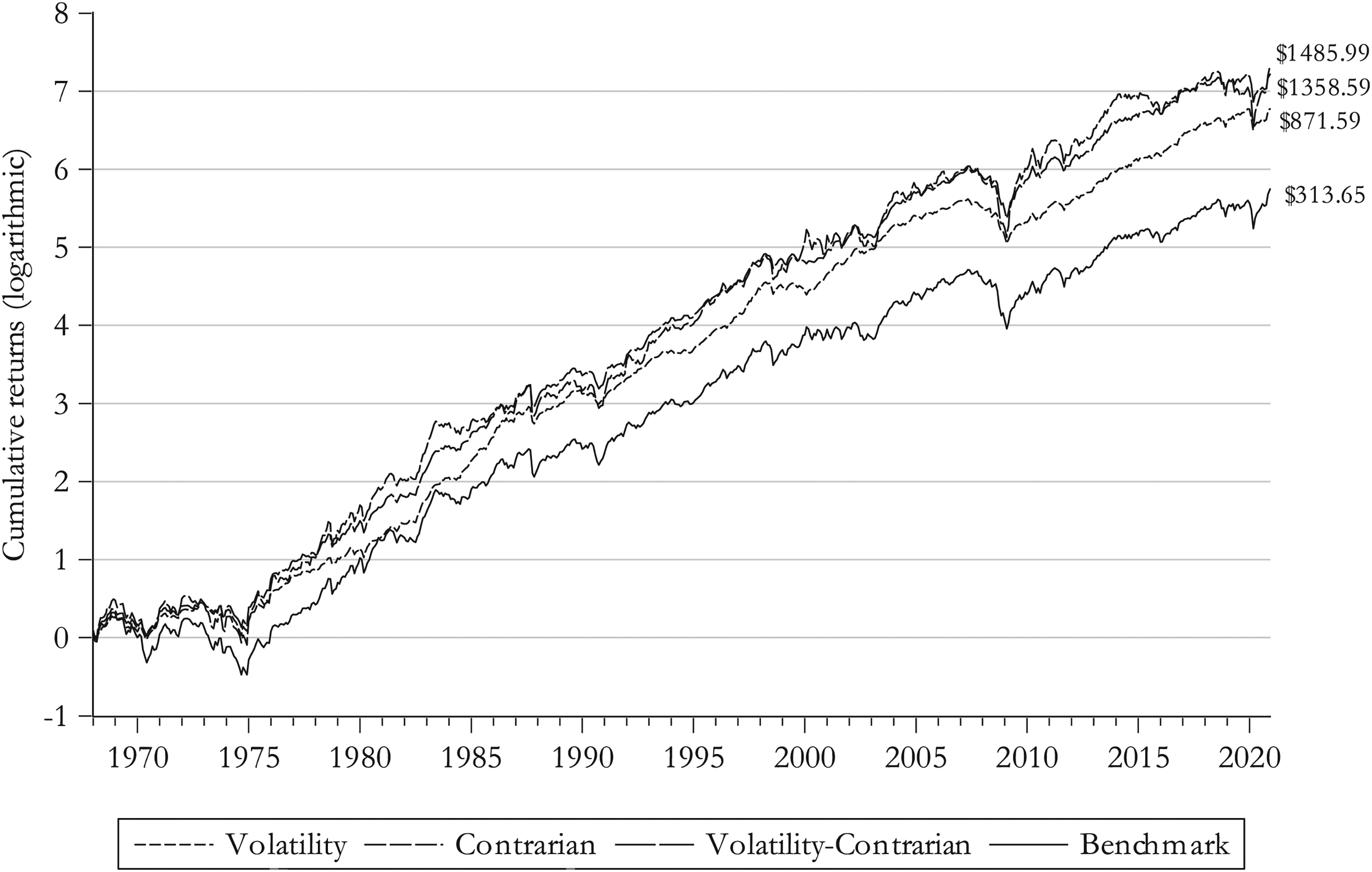
The LN-scaled return accumulation of the benchmark portfolio and the three best-within-style portfolios. Over the sample period from 1968:01 to 2020:12, LN-scaled net return accumulation is shown for the equally-weighted benchmark portfolio and for the three cost-mitigated long-only portfolios, which are monthly-updated low-volatility portfolio, annually-updated contrarian portfolio, and annually-updated double-sort portfolio consisting of contrarian stocks picked from the sub-set of below-median volatility stocks. For each portfolio, the terminal values at the end of December 2020 for the $1 initial investment made at the beginning of January 1968 are shown on the right.

Unsurprisingly, the return-generation pattern of the double-sort portfolio stands somewhere in between these two single-sort portfolios. With respect to volatility, the double-sort portfolio is closer to low-volatility portfolios, whereas in terms of net returns, it is closer to the contrarian portfolio. Although the annualized return differences are not big, the cumulative return differences grow big in the long term: For example, the cumulative return difference between the annually-updated contrarian portfolio and the monthly-updated low-volatility portfolio is over 70% during the 53-year holding period, implying that after transaction costs, the one-dollar initial investment in the monthly-updated low-volatility portfolio would have grown to a $871.59 terminal value, whereas the corresponding terminal value for the annually-updated contrarian portfolio would have ended up at $1.486. On the other hand, in the case of investing in an equally-weighted (value-weighted¹⁶) benchmark portfolio, the terminal value without any trading-cost reduction would have been approximately $313.6 ($190.6).

4.2. 6-factor exposures

Beside 6-factor alphas (reported in Table 2), the Fama-French-Carhart regression model reveals interesting information about factor exposures of the examined portfolios (Table 3). In general, the variability of excess returns of cost-mitigated portfolios are well explained by the variability of the six factor returns, as the lowest adjusted R² (reported for the annually-updated low-volatility portfolio) is 85.9%, implying that only 14.1% of the excess return variability remains unexplained by these factors in the worst case. At its best (in the case of the semiannually-updated double-sort portfolio), only 5.5% of the excess return variability remains unexplained.

Table 3.
Fama-French-Carhart 6-factor exposures for the bottom-quantile portfolios

Indicator adj. R2 MKT-RF SMB HML RMW CMA UMD

Panel A: 1-month holding period

36M s 86.6% 0.687^* –0.304^* 0.240^* 0.179^* 0.125^* 0.003

60M-12M 90.8% 1.101^* 0.240^* 0.081 –0.244^* 0.241^** –0.137^*

double-sort 94.3% 0.831^* –0.134^* 0.262^* 0.178^* 0.182^* –0.042^**

Panel B: 6-month holding period

36M s 86.5% 0.699^* –0.319^* 0.245^* 0.165^* 0.111^** –0.001

60M-12M 91.8% 1.093^* 0.245^* 0.057 –0.260^* 0.211^ –0.106^

double-sort 94.5% 0.854^* –0.149^* 0.261^* 0.172^* 0.167^* –0.035^**

Panel C: 12-month holding period

36M s 85.9% 0.706^* –0.314^* 0.233^* 0.167^* 0.130^* –0.009

60M-12M 91.8% 1.099^* 0.218^* 0.093^*** –0.208^* 0.181^* –0.097^

double-sort 93.9% 0.872^* –0.142^* 0.253^* 0.171^* 0.176^* –0.046^**

Indicator	adj. R2	MKT-RF	SMB	HML	RMW	CMA	UMD
Panel A: 1-month holding period
36M s	86.6%	0.687^*	–0.304^*	0.240^*	0.179^*	0.125^*	0.003
60M-12M	90.8%	1.101^*	0.240^*	0.081	–0.244^*	0.241^**	–0.137^*
double-sort	94.3%	0.831^*	–0.134^*	0.262^*	0.178^*	0.182^*	–0.042^**
Panel B: 6-month holding period
36M s	86.5%	0.699^*	–0.319^*	0.245^*	0.165^*	0.111^**	–0.001
60M-12M	91.8%	1.093^*	0.245^*	0.057	–0.260^*	0.211^**	–0.106^**
double-sort	94.5%	0.854^*	–0.149^*	0.261^*	0.172^*	0.167^*	–0.035^**
Panel C: 12-month holding period
36M s	85.9%	0.706^*	–0.314^*	0.233^*	0.167^*	0.130^*	–0.009
60M-12M	91.8%	1.099^*	0.218^*	0.093^***	–0.208^*	0.181^***	–0.097^**
double-sort	93.9%	0.872^*	–0.142^*	0.253^*	0.171^*	0.176^*	–0.046^**

Note. For the cost-mitigated bottom-quantile portfolios formed on the three portfolio-formation criteria named in the first column, shown are the slopes for each of the six factors and the adjusted coefficients of determination calculated on the basis of 636 monthly returns from January 1968 to December 2020. Panel A shows the results for monthly re-formed portfolios, whereas Panel B (C) shows the results for the portfolios that have been re-formed semi-annually (annually). The significance of the t-statistics for the factor slopes is calculated on the basis of the Newey-West (1987) HAC-adjusted standard errors and shown at the 1%, 5%, 10% level by ^*, ^**, and ^***, respectively.

The slopes for the market excess return factor range from 0.687 for the monthly-updated low-volatility portfolio to 1.101 for the corresponding contrarian portfolio, unsurprisingly being highly significant for every cost-mitigated portfolio.¹⁷ In general, the market excess return factor slopes are relatively even for each investment strategy regardless of holding period length, being clearly the lowest for low-volatility portfolios, and the highest for contrarian portfolios. Interestingly, all the SMB slopes are also highly significant, but with the notable difference that all low-volatility as well as double-sort portfolios are tilted towards large-caps, whereas all contrarian portfolios have reverse size (i.e., small-cap) tilt.¹⁸ Significantly negative SMB slopes of double-sort portfolios are explained by the order employed in sorts: Because volatility is used as the first-stage criterion, it likely excludes the majority of small-caps from the bottom-half volatility-sorted portfolio, from which the quintile of most contrarian stocks is extracted for double-sort portfolios. Therefore, double-sort portfolios are more liquid than contrarian portfolios, as well as less vulnerable to market frictions stemming from restricted investment capacity.

Unlike SMB slopes, all HML slopes are positive, being highly significant for low-volatility and double-sort portfolios regardless of holding period length. These findings are not surprising in light of earlier evidence on relationship between low-volatility and value effects (see, e.g., Chow et al., 2011; Scherer, 2011; Goldberg et al., 2014). By contrast, none of the HML slopes of contrarian portfolios is significant at the 5% level, although for the annually-updated contrarian portfolio, it is weakly significant (at better than the 10% level). These findings are somewhat surprising considering that earlier literature has drawn parallels between value and contrarian strategies (e.g., see Lakonishok et al., 1994; Asness et al., 2013). However, divergent results are explained by the fact that the linkage between contrarian stocks and value-growth factor exposures has changed and varied over time, having been at its strongest during the first decade of our sample period (This was verified by a robustness check, in which we removed the first 10 years of the sample data. Consequently, no significant relation between contrarian profits and value tilts is left for the remaining 43-year period from January 1978 to December 2020).

The RMW slopes behave inversely to the SMB slopes, being highly significant for all the examined portfolios, but positive for all low-volatility and double-sort portfolios, and negative for all contrarian portfolios. Significant tilts towards weaker profitability (or unprofitable) firms would indicate that if the contrarian stocks had been the stocks of potential turnaround companies, the turnarounds would not yet have materialized in terms of operating profitability within the year following the portfolio formation. The explanation for why the signs of RMW slopes of double-sort portfolios follow the slope signs of low-volatility instead those of contrarian portfolios, is similar to what was given for the sign variability of SMB slopes: Because low-volatility is positively related to high operating profitability (see also Fama and French, 2016, for earlier U.S. evidence), the first-stage sort based on volatility excludes the majority of the stocks of weakly profitable companies from the remaining stock universe, from which the examined double-sorted portfolios are formed.

The behavior of the CMA slopes is reminiscent of the HML slopes in the respect that they are all positive, thereby indicating that all the examined portfolios are tilted toward firms following conservative, rather than aggressive, investment policy. In addition, the CMA slopes are significant at the 5% level, except for the case of the annually-updated contrarian portfolio, where it is only weakly significant (at better than the 10% level). With respect to the relation between low-volatility portfolios and CMA exposures, our results are in line with Fama and French (2016). It is also expectable that the contrarian portfolios are tilted towards conservative asset-growth firms, as prior-loser firms have generally fewer incentives and/or chances to expand their business than have prior-winner firms (see, e.g. Garcia-Feijóo and Jensen, 2014).

Among the six factors included in the Fama-French-Carhart asset pricing model, the momentum factor is the only one, to which low-volatility portfolios do not have a significant exposure. By contrast, both contrarian and double-sort portfolios have a significantly negative UMD slope, thereby indicating that all these portfolios are tilted towards prior-year losers, rather than prior-year winner stocks. Because low-volatility portfolios are statistically neutral in terms of momentum exposures, the signs of the UMD slopes of the double-sort portfolios are, in this case, determined by the corresponding slope signs of contrarian portfolios. Altogether, a large proportion of significant factor exposures show that the employed simple portfolio-formation criteria derived only from past returns can offer a shortcut to style-diversified equity portfolios. In addition, our results provide long-term evidence that by following these simple strategies, an investor could have earned relatively small, but still statistically significant, abnormal returns.

4.3. Sub-period performance comparisons

4.3.1. Performance comparison for 26 and 1/2-year sub-periods

Because the recent literature has shown that anomalies tend to attenuate after their documentation (e.g., see McLean and Pontiff, 2016; Jones and Pomorski, 2017), we next examine whether this post-publication decline also holds on a long-only basis for the low-volatility and mean-reversion anomalies, and in addition, whether the portfolios formed on the related double-sort criterion could offer a better hedge against the attenuation than the single-sorted the low-volatility or contrarian strategies. First, we divide the 53-year period into two consecutive 26 and 1/2-year sub-periods and calculate the corresponding net returns and the Sharpe ratios, as well as the 6-factor alphas for each of cost-mitigated bottom-quantile portfolios being examined. To take a closer look at the time-variability of the relative performance of the quantile portfolios, we decompose the full sample period into five shorter sub-periods so that the first three of them include 11 years, whereas the last two include 10 years. For each portfolio-formation criterion, Table 4 shows the sub-period results for the monthly-updated low-volatility portfolio (in Panel A), and for the annually-updated contrarian and double-sort portfolios (in Panels B and C, respectively).¹⁹ In addition, the sub-period returns and the Sharpe ratios of monthly- and annually-updated benchmark portfolios are shown in the two rightmost columns in Panels A and B, respectively.

Table 4.
Sub-period performance statistics for the best-performing style portfolios

Sub -period NR (%) SR p value (%) α (%) Benchmark return (%) SR

Panel A: Low-volatility portfolio (monthly updating)

1968:01-1994:06 14.74 0.639 (0.0) 2.85^* 11.36 0.306

1994:07-2020:12 12.53 0.951 (0.5) 2.91^* 10.81 0.570

1968:01-1978:12 9.15 0.285 (4.4) 3.29^** 4.99 0.071

1979:01-1989:12 22.23 1.076 (0.2) 3.09^* 18.34 0.547

1990:01-2000:12 13.70 0.968 (11.6) 0.48 12.33 0.502

2001:01-2010:12 9.19 0.674 (19.8) 1.57 8.54 0.414

2011:01-2020:12 13.50 1.143 (0.5) 4.66^* 11.72 0.683

Panel B: Contrarian portfolio (annual updating)

1968:01-1994:06 16.06 0.477 (0.2) 0.51 11.83 0.333

1994:07-2020:12 13.50 0.571 (34.2) 2.61 11.07 0.541

1968:01-1978:12 12.31 0.352 (0.2) 0.09 5.88 0.105

1979:01-1989:12 19.30 0.579 (89.0) 0.11 18.44 0.565

1990:01-2000:12 16.71 0.650 (25.5) 6.59^* 13.21 0.568

2001:01-2010:12 14.82 0.591 (1.7) 3.72 8.25 0.414

2011:01-2020:12 10.56 0.532 (13.3) –1.48 11.62 0.704

Panel C: Double-sort portfolio (annual updating)

1968:01-1994:06 16.60 0.635 (0.0) 2.20^**

1994:07-2020:12 12.59 0.769 (2.8) 1.91^*

1968:01-1978:12 11.66 0.387 (0.1) 1.47

1979:01-1989:12 22.11 0.871 (0.2) 2.18^

1990:01-2000:12 14.53 0.843 (10.6) 1.91^*

2001:01-2010:12 12.43 0.723 (1.1) 2.48^**

2011:01-2020:12 12.07 0.813 (28.7) 3.30^*

Sub -period	NR (%)	SR	p value (%)	α (%)	Benchmark return (%)	SR
Panel A: Low-volatility portfolio (monthly updating)
1968:01-1994:06	14.74	0.639	(0.0)	2.85^*	11.36	0.306
1994:07-2020:12	12.53	0.951	(0.5)	2.91^*	10.81	0.570
1968:01-1978:12	9.15	0.285	(4.4)	3.29^**	4.99	0.071
1979:01-1989:12	22.23	1.076	(0.2)	3.09^*	18.34	0.547
1990:01-2000:12	13.70	0.968	(11.6)	0.48	12.33	0.502
2001:01-2010:12	9.19	0.674	(19.8)	1.57	8.54	0.414
2011:01-2020:12	13.50	1.143	(0.5)	4.66^*	11.72	0.683
Panel B: Contrarian portfolio (annual updating)
1968:01-1994:06	16.06	0.477	(0.2)	0.51	11.83	0.333
1994:07-2020:12	13.50	0.571	(34.2)	2.61	11.07	0.541
1968:01-1978:12	12.31	0.352	(0.2)	0.09	5.88	0.105
1979:01-1989:12	19.30	0.579	(89.0)	0.11	18.44	0.565
1990:01-2000:12	16.71	0.650	(25.5)	6.59^*	13.21	0.568
2001:01-2010:12	14.82	0.591	(1.7)	3.72	8.25	0.414
2011:01-2020:12	10.56	0.532	(13.3)	–1.48	11.62	0.704
Panel C: Double-sort portfolio (annual updating)
1968:01-1994:06	16.60	0.635	(0.0)	2.20^**
1994:07-2020:12	12.59	0.769	(2.8)	1.91^*
1968:01-1978:12	11.66	0.387	(0.1)	1.47
1979:01-1989:12	22.11	0.871	(0.2)	2.18^**
1990:01-2000:12	14.53	0.843	(10.6)	1.91^***
2001:01-2010:12	12.43	0.723	(1.1)	2.48^**
2011:01-2020:12	12.07	0.813	(28.7)	3.30^*

Note. For each sub-period (whose starting and end points are denoted as YYYY:MM–YYYY:MM in the first column), the table indicates the annualized geometric average net returns, the Sharpe ratios, and the Fama-French-Carhart 6-factor alphas (all annualized) for the cost-mitigated bottom-quantile portfolios formed on three portfolio-formation criteria. Panel A shows the performance statistics for the monthly-updated low-volatility portfolio, whereas the comparable statistics for the annually-updated contrarian and double-sort portfolios are shown in Panel B (C). Correspondingly, the two rightmost columns in Panel A (B) also show the geometric average return and Sharpe ratio of the monthly-updated (annually-updated) equally-weighted benchmark portfolio that consists of all NYSE-, AMEX- and NASDAQ-listed U.S. firms, whose stock price at the time of each portfolio formation has been equal to or higher than $5. The p values (in percentages in parentheses, determined on the basis of the Ledoit-Wolf (2008) test) indicate the significances for the Sharpe ratio differences between each quantile portfolio and the comparable equally-weighted benchmark portfolio. The significances of the 6-factor alphas at the 1%, 5%, 10% level are shown by ^*, ^**, and ^***, respectively.

The 26 and 1/2-year sub-period performance statistics do not show a clear attenuation tendency in performance for any of the examined portfolios (Table 4). Although net returns are considerably higher for the former sub-period from 1968:01 to 1994:06 for all the examined portfolios, the risk-adjusted post-cost performance statistics are actually better for the latter sub-period in many terms: For all three examined portfolios, the Sharpe ratios are higher for the latter sub-period. Particularly, the Sharpe ratio of the low-volatility portfolio for the latter sub-period is impressive, when taking account of the fact that according to literature, most anomalies seem to have disappeared during the post-millennium period (see, e.g., Arnott et al., 2019). For the examined portfolios, almost all the risk-adjusted performance statistics for the latter sub-period from 1994:07 to 2020:12 are better than the comparable statistics for the former sub-period of equal length. In this respect, the only exception is the 6-factor alpha of the double-sorted portfolio, as it is 0.29 percentage points higher for the former sub-period. However, the t statistics calculated for these sub-period alphas reveal that the latter sub-period alpha is more significant than the former. When interpreting the results, it should be noted that as a result of lower average risk-free rate, the Sharpe ratios of the benchmark portfolios are also higher for the latter than the former 26 and 1/2-year sub-period. Therefore, the significances of outperformance of the examined three portfolios against the benchmark have slightly deteriorated in terms of the Ledoit-Wolf test during the latter 26 and 1/2-year sub-period, remaining yet significant, except for the contrarian portfolio. Conversely, the significance levels of the 6-factor alphas have improved during the same period, although the greatest alpha documented for the contrarian portfolio is insignificant due to high standard error.

4.3.2. Performance comparison for shorter sub-periods

Although absolute returns of the examined portfolios over the benchmark have doubtlessly decreased during the latter 26 and 1/2-year sub-period, the risk-adjusted performance statistics do not tell the same story. However, the sub-period division into five shorter sub-periods reveals that both absolute and risk-adjusted returns have varied wildly during the 53-year sample period (see Table 4). Among these sub-periods at the aggregate level, the first 11-year period has been the worst in terms of both absolute and risk-adjusted returns, as the geometric average benchmark returns were only 5.88% p.a. (at annual rebalancing frequency) and 4.99% p.a. (at monthly rebalancing frequency), coupled with the corresponding Sharpe ratios of only 0.105 and 0.071, respectively. In spite of these challenging stock market conditions, all three examined portfolios generated significantly higher Sharpe ratio than the benchmark portfolio. By contrast, during the next 11-year sub-period from 1979:01 to 1989:12, the low-volatility portfolio significantly outperformed the benchmark portfolio, whereas the contrarian portfolio failed to do so in statistical sense. For the same sub-period, the double-sort portfolio generated a high net return of 22.11% p.a., which is very close to the corresponding return for the low-volatility portfolio. In terms of risk-adjusted returns, the margin in favor of the low-volatility portfolio is greater.

During the next 11-year sub-period from 1990:01 to 2000:12, the low-volatility portfolio did not manage to significantly outperform the benchmark portfolio in any terms, in spite of its spectacular Sharpe ratio of 0.968. At the same time, the contrarian portfolio generated the highest overall alpha of 6.59% p.a., which is highly significant as well. When these two single-sort portfolio-formation criteria were employed sequentially for 2×5 double-sorts, the overall performance statistics for this specific sub-period looks fine, although the 6-factor alpha is only weakly significant (at the 9.3% level).

Over the subsequent 10-year period from 2001:01 to 2010:12, the benchmark return was low at 8.25% p.a. (8.54 p.a.) with annual (monthly) rebalancing frequency, but the contrarian portfolio managed to significantly outperform the benchmark portfolio in terms of the Ledoit-Wolf test, coupled with a huge return margin of 6.55 percentage points p.a to the benchmark portfolio. Also, its 6-factor alpha is high in relative terms, although it is not significant due to its high standard error. For the low-volatility portfolio, this sub-period has been challenging particularly in terms of absolute returns, but when coupled with the contrarian indicator, the resulting double-sort portfolio has generated excellent performance statistics: It significantly outperformed the benchmark portfolio in terms of the Sharpe ratio difference, and also generated a statistically significant 6-factor alpha. Moreover, its net return was 4.18% p.a. higher than the gross return of the benchmark portfolio.

The last 10-year sub-period from 2011:01 to 2020:12 differs from its predecessor in many respects: Within this timespan, the performance statistics of the low-volatility portfolio is particularly impressive in all terms: Its annualized Sharpe ratio is spectacular at 1.143 and significantly higher than that of the benchmark portfolio. Besides that, its alpha is also excellent at 4.66% p.a., being highly significant as well. At the same time, the contrarian portfolio has performed poorly, as its Sharpe ratio is clearly, though not significantly lower than that of the benchmark portfolio. Its alpha is also negative, while simultaneously being insignificant. When the mean-reversion ranking is conditioned on the volatility ranking in 2×5 sequential double-sorts, the performance statistics become much better (in comparison to that of the single-sort contrarian portfolio) to the extent that the double-sort portfolio generates highly significant alpha of 3.30% p.a. Nevertheless, the unambiguous winner of this sub-period, which has generally been very challenging for any investor trying to exploit previously-documented equity anomalies, is the low-volatility portfolio.

The previously-described sub-period results reveal that the double-sort portfolio-formation can offer important style-diversification benefits because of a long-horizon tendency of low-volatility and mean-reversion strategies to “shine” and “fall short” at different times: When low-volatility performs poorly, the double-sort portfolio is carried over by a good performance of the contrarian portfolio. Although there are periods during which the outperformance of the double-sort portfolio against the benchmark portfolio is not significant in all terms, the efficacy of this double-sort criteria is clearly evident in Panel C of Table 4.

4.3.3. Factor exposures over sub-periods

The sub-period regressions also reveal some interesting insights to behavior of factor exposures over time. Table 5 shows the regression slopes of the six factors for the examined sub-periods for the same bottom-quantile portfolios that are included in Table 4. The sub-period slopes for the market excess return factor are consistent with the full-sample-period slopes in respect that for all the examined sub-periods, they are lowest for the low-volatility portfolio, while being highest for the contrarian portfolios. The sub-period SMB slopes are also consistent with the corresponding full-sample-period slopes, indicating that large-cap tilt of the low-volatility portfolio has been persistent, whereas the contrarian portfolios has been more or less tilted towards small-caps. The same also holds for the double-sort portfolio, for which a slightly deteriorating significance of negative SMB slope towards the present is observed.

Table 5.
Fama-French-Carhart 6-factor exposures for the sub-periods

Sub -period MKTRF SMB HML RMW CMA UMD

Panel A: Monthly-updated 36M σ bottom-quantile portfolio

1968:01-1994:06 0.752^* –0.437^* 0.350^* 0.078 –0.027 –0.073^**

1994:07-2020:12 0.651^* –0.239^* 0.196^* 0.226^* 0.154 0.025

1968:01-1978:12 0.772^* –0.507^* 0.365^ 0.048 –0.040 –0.141^

1979:01-1989:12 0.757^* –0.353^* 0.500^* 0.165^* –0.19^* –0.038

1990:01-2000:12 0.687^* –0.303^* 0.286^* 0.173^* 0.154^** 0.003

2001:01-2010:12 0.565^* –0.111^*** 0.191^* 0.118^** 0.174^* 0.015

2011:01-2020:12 0.687^* –0.198^* 0.183^** 0.237^* 0.093 0.139^*

Panel B: Annually-updated 60M-12M bottom-quantile portfolio

1968:01-1994:06 1.098^* 0.286^* 0.212^ 0.023 0.318^ –0.029

1994:07-2020:12 1.131^* 0.196^ –0.012 –0.141^ 0.151 –0.135^**

1968:01-1978:12 1.178^* 0.204 0.440^* 0.398^* 0.386^** 0.014

1979:01-1989:12 1.040^* 0.134^* –0.095 –0.217^** 0.415^* –0.040

1990:01-2000:12 1.010^* 0.223^** 0.116 –0.347^* 0.064 –0.130^**

2001:01-2010:12 1.148^* 0.289^ –0.047 0.013 0.081 –0.152^

2011:01-2020:12 1.234^* 0.042 –0.039 –0.184 0.325^** –0.167^*

Panel C: Annually-updated double-sort bottom-quantile portfolio

1968:01-1994:06 0.930^* –0.214^** 0.304^* 0.118^ 0.170^ –0.065^***

1994:07-2020:12 0.824^* –0.089^* 0.226^* 0.213^* 0.135^* –0.053^*

1968:01-1978:12 0.969^* –0.324^* 0.506^* 0.314^** 0.184 –0.071

1979:01-1989:12 0.933^* –0.216^* 0.235^* 0.087 0.082 –0.0071^***

1990:01-2000:12 0.826^* –0.061^*** 0.260^* 0.168^* 0.125 –0.140^*

2001:01-2010:12 0.826^* –0.076^*** 0.213^* 0.191^* 0.194^* –0.040^***

2011:01-2020:12 0.834^* –0.074 0.237^* 0.068 0.086 0.006

Sub -period	MKTRF	SMB	HML	RMW	CMA	UMD
Panel A: Monthly-updated 36M σ bottom-quantile portfolio
1968:01-1994:06	0.752^*	–0.437^*	0.350^*	0.078	–0.027	–0.073^**
1994:07-2020:12	0.651^*	–0.239^*	0.196^*	0.226^*	0.154	0.025
1968:01-1978:12	0.772^*	–0.507^*	0.365^**	0.048	–0.040	–0.141^**
1979:01-1989:12	0.757^*	–0.353^*	0.500^*	0.165^***	–0.19^***	–0.038
1990:01-2000:12	0.687^*	–0.303^*	0.286^*	0.173^*	0.154^**	0.003
2001:01-2010:12	0.565^*	–0.111^***	0.191^*	0.118^**	0.174^*	0.015
2011:01-2020:12	0.687^*	–0.198^*	0.183^**	0.237^*	0.093	0.139^*
Panel B: Annually-updated 60M-12M bottom-quantile portfolio
1968:01-1994:06	1.098^*	0.286^*	0.212^**	0.023	0.318^**	–0.029
1994:07-2020:12	1.131^*	0.196^**	–0.012	–0.141^**	0.151	–0.135^**
1968:01-1978:12	1.178^*	0.204	0.440^*	0.398^*	0.386^**	0.014
1979:01-1989:12	1.040^*	0.134^*	–0.095	–0.217^**	0.415^*	–0.040
1990:01-2000:12	1.010^*	0.223^**	0.116	–0.347^*	0.064	–0.130^**
2001:01-2010:12	1.148^*	0.289^**	–0.047	0.013	0.081	–0.152^**
2011:01-2020:12	1.234^*	0.042	–0.039	–0.184	0.325^**	–0.167^*
Panel C: Annually-updated double-sort bottom-quantile portfolio
1968:01-1994:06	0.930^*	–0.214^**	0.304^*	0.118^**	0.170^**	–0.065^***
1994:07-2020:12	0.824^*	–0.089^*	0.226^*	0.213^*	0.135^*	–0.053^*
1968:01-1978:12	0.969^*	–0.324^*	0.506^*	0.314^**	0.184	–0.071
1979:01-1989:12	0.933^*	–0.216^*	0.235^*	0.087	0.082	–0.0071^***
1990:01-2000:12	0.826^*	–0.061^***	0.260^*	0.168^*	0.125	–0.140^*
2001:01-2010:12	0.826^*	–0.076^***	0.213^*	0.191^*	0.194^*	–0.040^***
2011:01-2020:12	0.834^*	–0.074	0.237^*	0.068	0.086	0.006

Note. For the cost-mitigated bottom-quantile portfolios formed on the three portfolio-formation criteria named in the panel heading, shown are the slopes for each of the six factors calculated on the basis of 636 monthly returns from January 1968 to December 2020. The significance of the t-statistics for the factor slopes is calculated on the basis of the Newey-West (1987) HAC-adjusted standard errors and shown at the 1%, 5%, 10% level by ^*, ^**, and ^***, respectively.

The sub-period regression results confirm that the low-volatility portfolio has had a relatively stable positive HML exposure throughout the full sample period.²⁰ For the contrarian portfolio, the HML slopes have varied more: During the first 11-year and the 26 1/2-year periods, the contrarian portfolio has had significantly positive HML exposure, whereas during all the other examined sub-periods, its HML exposure has been insignificant and negative in most cases, thereby giving further evidence that the linkage between contrarian stocks and value-growth factor exposures has changed and varied over time. By contrast, the double-sort portfolio has had a highly significant value tilt in all the examined sub-periods, thereby indicating that the employed two-staged portfolio-formation criterion induces more value-like stocks being included in the double-sort portfolio than in cases of contrarian portfolios. Importantly, these significant value tilts do not absorb all abnormal returns as the 6-factor alphas of the double-sort portfolio are at least weakly significant for all the examined sub-periods, except for the first 11-year period 1968:01 to 1978:12.

The sub-period RMW slopes are all positive for the low-volatility and the double-sort portfolios, whereas for the contrarian portfolio, the sign of the RMW slopes varies across the sub-periods: For example, during the first 11-year sub-period from 1968:01 to 1978:12, the contrarian portfolio has had a highly significant tilt towards highly profitable stocks, whereas for the sub-period from 1990:01 to 2000:12, a reverse profitability exposure is documented. Moreover, for the former 26 and 1/2-year sub-period, the RMW slope does not deviate significantly from zero, whereas during the latter, the contrarian portfolio has had a significant low-profitability tilt.

Unlike RMW slopes, the sub-period CMA slopes are all positive for the contrarian portfolio, whereas for the low-volatility portfolio, their signs vary across the sub-periods. This shows that the CMA exposure of the low-volatility strategy is not so straightforward that could be inferred from the full sample period results. Particularly, during the first half of the sample period, the explanatory power of the CMA factor on low-volatility returns has been weak.²¹ Somewhat surprisingly, the CMA slopes of double-sort portfolio are positive for all the examined sub-periods, indicating that CMA exposures are determined more on the basis of the second-stage rather than based on the first-stage criterion. However, although the CMA slope of the double-sort portfolio is significant for both 26 and 1/2-year sub-periods, it is insignificant for all other shorter sub-periods examined, except for the 10-year sub-period from 2001:01 to 2010:12.

The sub-period UMD slopes are mostly negative, with a notable exception that during the last 10-year sub-period, the low-volatility portfolio has had a highly significant positive momentum tilt. By contrast, its UMD exposure during the first 11-year sub-period from 1968:01 to 1978:12, as well as during the first 26 and 1/2-year sub-period, has been significantly negative. These findings are consistent with the results of Garcia-Feijóo et al. (2015) who also show that momentum exposure of low-volatility strategies varies over time. Unlike the SMB slopes, the UMD slopes do not systematically differ between the low-volatility and contrarian portfolios. All the sub-period UMD slopes of the double-sort portfolio except that for the last 10-year sub-period, are negative, although only for the latter 26 and 1/2-year sub-period and for the 11-year sub-period from 1990:01 to 2000:12, the UMD slopes are statistically significant at better than the 5% level.

4.4. Performance decomposition

To find out whether the differences in the sensitivity to rising or declining stock market returns explain the performance differences between the quintile portfolios, we divide the full sample period into bullish and bearish months based on the sign of the market return [calculated from the first Fama-French (1993) factor (i.e., market excess return)], similar to Fuller and Goldstein (2011). Based on that criterion, the full 53-year sample period includes 396 bullish and 240 bearish months. Table 6 shows geometric averages of monthly excess returns [above (+) or below (–) the sample average and in percentages] during the up- and down-market months. The results reveal a remarkable difference in excess return generation patterns between low-volatility and contrarian portfolios: During the bearish months, the low-volatility stocks lose far less of their value than do the stocks on average, whereas in bullish months, they lag significantly behind the stock market average. In line with the results of Blitz and van Vliet (2007), the underperformance of low-volatility stocks during bullish months is considerably less than their outperformance during bearish months, although this effect is partially countered by more frequent occurrence of bullish months (62.2% of all sample months). By contrast, the excess returns of the contrarian portfolios are clearly positive during bullish months (in the case of annually-updated contrarian portfolio, the excess return is also significantly positive at better than the 5% level), while being insignificantly negative in bearish months. Unsurprisingly, the excess returns of double-sort portfolios behave more like those of low-volatility portfolios, being however, far less negative during bullish months, as well as considerably less positive during bearish months. For all nine portfolios, excess return differences between up-market and down-market months are statistically significant. Although their excess return generation is dependent on the direction of overall stock market development, the direction of the dependency is opposite in the case of contrarian portfolios compared to cases of low-volatility and double-sort portfolios.

Table 6.
Performance decomposition statistics

Indicator Up-market months Down-market months Bullish period Bearish period Expansive monetary state Restrictive monetary state Expansion months Recession months MDD Recovery time (months)

Panel A: 1-month holding period

36M –1.25^* 2.42^* –0.29 2.08^* –0.57 0.38 0.18 0.58 –43.37 36

60M-12M 0.54^*** –0.46 0.23 –0.23 0.66 0.01 0.18 0.28 –67.17 24

double-sort –0.68^* 1.57^* –0.10 1.42^*** –0.20 0.31 0.22 0.49 –50.63 24

Panel B: 6-month holding period

36M –1.30^* 2.43^* –0.32 2.07^* –0.56 0.34 0.15 0.61 –42.49 37

60M-12M 0.52^*** –0.31 0.26 –0.07 0.56 0.10 0.24 0.32 –63.79 14

double-sort –0.67^* 1.60^* –0.09 1.49^** –0.17 0.32 0.24 0.50 –48.75 23

Panel C: 12-month holding period

36M –1.22^* 2.20^* –0.31 1.84^* –0.52 0.15 0.01 0.76 –40.40 36

60M-12M 0.63^** –0.34 0.31 –0.01 0.62 0.28 0.17 0.67 –59.77 12

double-sort –0.51 1.38^* –0.04 1.32^*** –0.08 0.31 0.15 0.73 –47.58 14

Indicator	Up-market months	Down-market months	Bullish period	Bearish period	Expansive monetary state	Restrictive monetary state	Expansion months	Recession months	MDD	Recovery time (months)
Panel A: 1-month holding period
36M	–1.25^*	2.42^*	–0.29	2.08^*	–0.57	0.38	0.18	0.58	–43.37	36
60M-12M	0.54^***	–0.46	0.23	–0.23	0.66	0.01	0.18	0.28	–67.17	24
double-sort	–0.68^*	1.57^*	–0.10	1.42^***	–0.20	0.31	0.22	0.49	–50.63	24
Panel B: 6-month holding period
36M	–1.30^*	2.43^*	–0.32	2.07^*	–0.56	0.34	0.15	0.61	–42.49	37
60M-12M	0.52^***	–0.31	0.26	–0.07	0.56	0.10	0.24	0.32	–63.79	14
double-sort	–0.67^*	1.60^*	–0.09	1.49^**	–0.17	0.32	0.24	0.50	–48.75	23
Panel C: 12-month holding period
36M	–1.22^*	2.20^*	–0.31	1.84^*	–0.52	0.15	0.01	0.76	–40.40	36
60M-12M	0.63^**	–0.34	0.31	–0.01	0.62	0.28	0.17	0.67	–59.77	12
double-sort	–0.51	1.38^*	–0.04	1.32^***	–0.08	0.31	0.15	0.73	–47.58	14

Note. For the sample of non-penny U.S. stocks and each of the three holding-period lengths employed, Table 5 shows monthly geometric average excess returns (over the holding-period-specific benchmark portfolio, in percentages) net of transaction costs over the up- and down-market months (determined on the basis of the sign of U.S. stock market returns), bull and bears states (by using cumulative threshold percentages of +20% and –15% for demarcating bull and bear states, respectively), over the expansive and restrictive monetary states (defined as in Jensen and Moorman, 2010), as well as over the expansionary and recessionary periods (defined on the basis of the NBER recession dates from the Federal Reserve Bank of St. Louis’ website). The p values indicating significant non-zero excess returns at the 1%, 5%, and 10% level are denoted by ^*, ^**, and ^***, respectively. In addition, maximum drawdown statistics (MDD in percentages) and recovery times from the MDDs (in terms of the number of months passed from the trough and required for exceeding the peak at the start point of MDD) are shown. The statistics are shown for the nine cost-mitigated bottom-quantile portfolios formed on three portfolio-formation criteria (named in the first column). Panel A shows the results for monthly-updated portfolios, whereas the corresponding statistics for the portfolios re-formed semi-annually (annually) are shown in Panel B (C).

As a supplementary robustness check for the dependency of relative performance of the trading portfolios on the stock market trend, we also divided the sample period into bull and bear market periods according to the turning points of the U.S. stock market, by using a cumulative return (loss) from the previous trough (peak) to the subsequent peak (trough) in the demarcation of market turns. The corresponding threshold percentages for bull and bear states are +20% and –15%, respectively.²²Table 6 shows that results of this analysis are parallel to, although not as striking as those based on the division on the bullish and bearish months. Because of bullish (bearish) months included in bearish (bullish) periods, the excess returns are more conservative than in the case, where the demarcation of months is based on just the sign of the market return. Consequently, statistically significant excess returns are less frequent in market-state analysis, occurring only in bear states in cases of low-volatility and double-sort portfolios. Also, excess return differences between bullish and bearish months are statistically significant for the same portfolios, thereby indicating their bearish-period outperformance tendency, whereas for contrarian portfolios, the corresponding differences are insignificant for all three updating frequencies.

Motivated by the results of Garcia-Feijóo and Jensen (2014), according to whom the prices of past loser (i.e., contrarian) stocks only rebound during expansive monetary conditions, we also test whether the excess return generation for the examined trading portfolios is conditional on the monetary environment. Following Jensen and Moorman (2010), we form a binary monetary-conditions score on the basis of two monetary policy indicators. The first of these is based on changes in the federal funds rate, which has been widely used for identifying adjustments in Fed stringency in the short-term money markets (see, e.g., Patelis, 1997; Perez-Quiros and Timmermann, 2000). The second indicator is based on changes in the Fed discount rate, which has been used to identify fundamental shifts in the Fed’s broad policy stance (see, e.g., Jensen, Mercer, and Johnson, 1996; Conover et al., 2005).

For both of these policy rates, downward changes are interpreted as signals of loosening monetary policy, whereas upward changes represent a tightening monetary environment. The months are divided into two groups of expansive and restrictive conditions based on the directional changes of these rates. The monetary environment is classified as expansive (restrictive) if both rates decrease (increase) from month t –1 to month t. If the rates move into opposite directions, monetary conditions are considered restrictive. For months in which neither of policy rates change, the existing monetary condition remains. In line with Jensen and Moorman (2010), the change in the Fed’s broad policy stance also necessitates a directional change in the Fed discount rate.

The excess return statistics conditioned on the monetary environment (Table 6) shows that the return generation patterns differ most radically in expansive conditions, during which the contrarian portfolios have generated clearly above-benchmark returns.²³ Conversely, the excess returns of low-volatility portfolios are almost as clearly negative in similar conditions. However, neither of these excess returns is statistically significant due to their high standard errors. By contrast, the corresponding excess return difference between contrarian and low-volatility portfolios is large enough for being weakly significant (at the 10% level). In restrictive conditions, none of the nine portfolios have generated significant non-zero excess returns, although their signs are positive for all the other portfolios except for the monthly-updated contrarian portfolio. Unsurprisingly, the dependence of excess return generation of double-sort portfolios on monetary conditions is closer to that of low-volatility portfolios than that of contrarian portfolios but with a desirable difference that in expansive conditions, the double-sort portfolios have lagged far less behind the benchmark than have the low-volatility portfolios. For the last-mentioned portfolios, excess return differences between expansive and restrictive monetary states are also statistically significant (at better than the 5% level) regardless of the holding-period length, whereas for the contrarian and double-sort portfolios, the corresponding differences are insignificant in all six cases.

A similar analysis as performed for bullish and bearish indicators as well as for monetary state indicators is repeated by dividing the full-length sample period into expansion and recession months determined on the basis of the NBER recession dates from the Federal Reserve Bank of St. Louis’ website²⁴ (see Table 6). In comparison to the division into bull- and bear-state periods, the pooled expansion period includes 482 (61) months that belong to the bull-state (bear-state) months, whereas the corresponding recession period consists of 31 bull-state and 62 bear-state months. The major difference between these two classifications is in that bear-state months are relatively evenly distributed between business cycles, whereas the bull-state months dominate the expansionary period. Compared to the other classifications used for performance decomposition, the classification based on business cycles reveals fewer differences in excess return generation between the portfolios, as excess returns are positive in both business cycles for all nine portfolios. Although excess returns are clearly more positive during recession periods than in expansionary periods, they are statistically insignificant for all portfolios even at their highest, implying that the excess return generation of all the examined nine portfolios is only loosely related to business cycles. Moreover, excess return differences between expansion and recession periods are statistically insignificant in all nine cases.

Inspired by earlier evidence for seasonality characteristics of contrarian profits, we test for all the portfolios, whether their excess return generation is dependent on calendar month (By subtracting monthly benchmark returns from the corresponding portfolio returns, we rule out the possibility of finding anomalous returns for a specific month just because of seasonality in monthly market returns). The (un-tabulated) results show that excess returns of all three contrarian portfolios have been significantly positive in January, whereas January excess returns of low-volatility portfolios have been clearly, though insignificantly negative.²⁵ For all other than contrarian portfolios as well as in all the other months than January, the excess returns are insignificant, implying that none of the remaining monthly excess returns has not significantly deviated from zero. The results also show that the January-return difference between contrarian and low-volatility portfolios more than fully explains their full-sample-period return difference. In other words, the low-volatility portfolios have earned on average higher returns than contrarian portfolios during the remaining 11 calendar months. Consequently, the excess return generation is much more even (discrete) across calendar months for double-sort portfolios than it is for contrarian and low-volatility portfolios.

4.5. The crash risk exposure

To find out whether the differences in crash risk exposures between the examined anomalous portfolios exist, we calculated the maximum drawdown (MDD) statistics (based on the month-end values of the portfolios) for all three bottom-quantile portfolios per each holding period length. Similar to Rujeerapaiboon, Kuhn, and Wiesemann (2016), MDD is defined as maximum percentage loss over any subinterval of the evaluation period. The penultimate column of Table 6 shows that regardless of the holding-period length, the differences in crash risk exposures between the examined investment strategies are remarkable: For all three holding-period lengths, the smallest MDDs are documented for the low-volatility portfolios, whereas the greatest MDDs are reported for the contrarian portfolios. For all three portfolio-formation criteria, the MDDs are greatest (smallest) for monthly-updated (annually-updated) portfolios. Although the MDDs are clearly smallest for the low-volatility portfolios, it is noteworthy that despite their defensive characteristic in this respect, it has taken three years until their peak values at the start point of MDD have been reached again. By contrast, the corresponding recovery times for contrarian and double-sorted portfolios are far shorter, although their MDD statistics are worse. The differences in recovery speed are greatest among annually-updated portfolios, as the recovery times for the contrarian and double-sort portfolios are only 12 and 14 months, respectively. For all the examined portfolios, the realization of MDD has taken place during the financial crisis period 2007–2009.

4.6. Robustness check in the non-microcap stock universe

As evident on the basis of the value-weighted quantile portfolio statistics reported at French’s data library, value-weighting attenuates particularly contrarian profits, and therefore, we have focused on an equal-weighted approach in portfolio formation, thereby leaving more room for the speculation whether our results are driven by tiny and illiquid stocks. Although setting the 5$ price filter for investable stocks excludes many tiny and illiquid stocks, it doesn’t exclude them all. Therefore, we made a robustness test by also excluding — beside the penny stocks — the so-called microcap companies, whose market capitalization at the start of each month investment period was below the bottom NYSE quintile breakpoint, following Avramov et al. (2007), and Pätäri et al. (2023), among others. On average, more than half of the firms on the NYSE, AMEX, and Nasdaq were excluded, while simultaneously losing only a small percentage of total market capitalization (e.g., see Fama and French, 2008; Hou et al., 2020).²⁶ The corresponding performance statistics for the cost-mitigated bottom-quantile portfolios is reported in Appendix A.

For all the examined investment strategies, the removal of microcaps from the investable universe of stocks somewhat attenuates all the reported performance metrics in absolute terms, but on the other hand, the performance statistics of semiannually- and annually-updated non-microcap benchmark portfolios also decrease slightly in comparison with that of the corresponding non-penny-stock benchmark portfolio. Consequently, the same portfolios that in terms of the Sharpe ratio significantly outperform their benchmark portfolio in the non-penny-stock universe, do the same in the universe of stocks, from which both penny stocks and microcap stocks are excluded. However, the same does not hold in terms of the 6-factor alphas which unsurprisingly lose more of their significances to the extent that only two statistically significant alphas are left: The 6-factor alpha of the monthly-updated volatility portfolio and that of the annually-updated contrarian portfolio remain statistically significant at better than the 10% level. Also in absolute terms, the 6-factor alphas attenuate more than the Sharpe ratios when the microcaps are excluded from the sample. This is expectable as microcap stocks have on average high idiosyncratic risk²⁷ that may not be captured as well by the factor spreads employed in the FFC 6-factor regression model as in the market-cap restricted universe. If this inherent tendency of multifactor alphas to shrink towards larger-cap universe of stocks is taken into account in the interpretation of the results, it can be concluded that the results for the non-microcap sample remain qualitatively the same as for the non-penny-stock sample. The same also holds for the factor exposures that are also reported in Appendix table for comparability purposes. Compared to the corresponding nine cost-mitigated non-penny-stock portfolios (reported in Table 2), the turnover rates are slightly lower in the non-microcap universe of stocks, but very consistent on the basis of vis-a-vis comparisons between these two samples, being at their lowest (highest) for annually-updated (monthly-updated) portfolios. As in the non-penny-stock universe, the turnover rates of low-volatility portfolios are outstandingly lower than those of contrarian or double-sort portfolios.

5. Conclusions

This paper contributes to the existing literature by analyzing the benefits of combining two distinct stock market anomalies, namely the low-volatility and mean-reversion anomalies. According to our post-cost results, by using the double-sort portfolio-formation criterion in which the contrarian stocks are picked from the sub-set of below-median volatility stocks, an investor can reduce the risk of intermediate-term below-market performance that has occasionally materialized for low-volatility investors. The added-value of low-volatility investing stems mostly from the risk-reduction side, rather than from the return-enhancement side, whereas contrarian stocks are generally highly volatile with a remarkable upside potential. By excluding above-median volatility stocks from the investment opportunity set, the risk-adjusted performance of long-only contrarian portfolios can be enhanced remarkably. Over the 53-year sample period, the annually-updated double-sort portfolio has been more stable (out)performer than the low-volatility portfolio, although the last ten years of the sample period from 2011:01 to 2020:12 have been particularly favorable for low-volatility investors. Combining low volatility and mean reversion is also useful in the respect that it helps to avoid small-cap tilt that is inherent in pure contrarian portfolios (Contrarian profits are driven by small-cap stocks).

The excess return generation of the contrarian low-volatility portfolio is also less dependent on market states than it is for pure low-volatility and contrarian portfolios. The outperformance of low-volatility portfolios stems from their tendency to decline far less than the market portfolio in bearish conditions, whereas in bullish conditions, they lag behind the market portfolio. By contrast, contrarian portfolios generate their excess returns (over the market portfolio) in bullish states, being relatively neutral compared to the average market portfolio return in bearish states. Consequently, the double-sorted contrarian low-volatility portfolio behaves similarly to the market portfolio in bull states while declining clearly less than the market portfolio in bear states. Because bull states are more common in stock markets than bear states, the double-sort portfolio generates higher long-term returns than low-volatility portfolios, being clearly less risky than pure contrarian portfolios.

Supplementary Material

Footnotes

Acknowledgments

We thank the editor (Philip Maymin) and the anonymous reviewer for their valuable comments on earlier drafts of this paper. We are also grateful to Olivier Ledoit, Michael Wolf, Andrew Patton, and Allan Timmermann for making their programming codes freely available. In addition, we are indebted to Ken French for free access to his data library. This research did not receive any specific grant from funding agencies in the public, commercial, or not-for-profit sectors.

Declarations of interest

None

Supplementary material

The Appendix is available in the electronic version of this article: .

Notes

References

Abdi

Ranaldo

2017. A simple estimation of bid-ask spreads from daily close, high, and low prices, Review of Financial Studies 304437–4479.

Arnott

Harvey

C.R.

Kalesnik

Linnainmaa

2019. Alice’s adventures in factorland: Three blunders that plague factor investing, Journal of Portfolio Management 45(4), 18–36.

Asness

C.S.

Moskowitz

T.J.

Pedersen

L.H.

2013. Value and momentum everywhere, Journal of Finance 68, 929–985.

Avramov

Chordia

Jostova

Philipov

2007. Momentum and credit rating, Journal of Finance 622503–2520.

Bali

T.G.

Cakici

2008. Idiosyncratic volatility and the cross section of expected returns, Journal of Financial and Quantitative Analysis 4329–58.

Baker

Bradley

Wurgler

2011. Benchmarks as limits to arbitrage: Understanding the low-volatility anomaly, Financial Analysts Journal 67(1), 40–54.

Barber

Odean

2008. All that glitters: The effect of attention and news on the buying behavior of individual and institutional investors, Review of Financial Studies 21785–818.

Beaver

W.H.

McNichols

Price

2007. Delisting returns and their effect on accounting-based market anomalies, Journal of Accounting and Economics 21341–368.

Beneish

M.D.

Lee

C.M.C.

Nichols

D.C.

2015. In short supply: Short-sellers and stock returns, Journal of Accounting and Economics 6033–57.

10.

Blitz

2016. The value of low volatility, Journal of Portfolio Management 42(3), 94–100.

11.

Blitz

2021. The quant crisis of: Cornered by big growth, Journal of Portfolio Management 47(6), 8–21.

12.

Blitz

Baltussen

van Vliet

2020. When equity factors drop their shorts, Financial Analysts Journal 76(4), 73–99.

13.

Blitz

Falkenstein

EG.

van Vliet

2013. Explanations for the volatility effect: An overview based on the CAPM assumptions, Journal of Portfolio Management 40(3)61–76.

14.

Blitz

Hanauer

MX.

Vidojevic

2020. The idiosyncratic momentum anomaly, International Review of Economics and Finance 69932–957.

15.

Blitz,

D.C.

van Vliet

2007. The volatility effect, Journal of Portfolio Management 34(1) 102–113.

16.

Blitz,

van Vliet

2018. The conservative formula: Quantitative investing made easy, Journal of Portfolio Management 44(7), 24–38.

17.

Blitz

van Vliet

Baltussen

2020. The volatility effect revisited, Journal of Portfolio Management 46(2)46–53.

18.

Carhart,

M.M.

1997. On persistence in mutual fund performance, Journal of Finance 5257–82.

19.

Chen

T.Y.

Chou

P.H.

K.C.

Rhee

S.G.

2021. Non-parametric momentum based on ranks and signs, Journal of Empirical Finance 6094–109.

20.

Chow

TM.

Hsu

Kalesnik

Little

2011. A survey of alternative equity index strategies, Financial Analysts Journal 67(5), 37–57.

21.

Chow

TM.

Hsu

JC.

Kuo

LL.

2014. A study of low-volatility portfolio construction methods, Journal of Portfolio Management 40(4), 89–105.

22.

Clarke

RG.

De Silva

Thorley

2006. Minimum-variance portfolios in the US equity market, Journal of Portfolio Management 33(1), 10–24.

23.

Cohen

Diether

KB.

Malloy

C.J.

2007. Supply and demand shifts in the shorting market, Journal of Finance 622061–2096.

24.

Conover

CM.

Jensen

GR.

Johnson

RR.

Mercer

J.M.

2005. Is Fed policy still relevant for investors? Financial Analysts Journal 61(1), 70–79.

25.

Daniel,

Titman

1997. Evidence on the characteristics of cross sectional variation in stock returns, Journal of Finance 521–33.

26.

Daniel,

Moskowitz

T.J.

2016. Momentum crashes, Journal of Financial Economics 122221–247.

27.

Davis,

EP.

Steil

2004. Institutional Investors. MIT press; Cambridge, Massachusetts.

28.

D’Avolio,

2002. The market for borrowing stock, Journal of Financial Economics 66271–306.

29.

DeMiguel

Garlappi

Uppal

2009. Optimal versus naive diversification: How inefficient is the 1/N portfolio strategy? Review of Financial Studies 221915–1953.

30.

De Bondt,

W.F. .

Thaler

1985. Does the stock market overreact? Journal of Finance 40793–805.

31.

De Bondt

W.F.

Thaler

1987. Further evidence on investor overreaction and stock market seasonality, Journal of Finance 42557–581.

32.

Di Maggio

Egan

Franzoni

2022. The value of intermediation in the stock market, Journal of Financial Economics 145208–233.

33.

van Dijk

, M.A.

2011. Is size dead? A review of the size effect in equity returns, Journal of Banking and Finance 353263–3274.

34.

Drechsler

Q.F.

2016. The shorting premium and asset pricing anomalies. Working paper. Available at https://ssrn.com/abstract=2387099.

35.

Edwards

Biscarri

JG.

de Gracia

F.P.

2003. Stock market cycles, financial liberalization and volatility, Journal of International Money and Finance 22925–955.

36.

Fama,

E.F.

1970. Efficient capital markets: A review of theory and empirical work, Journal of Finance 25383–417.

37.

Fama,

E.F.

French

K.R.

1993. Common risk factors in the returns on stock and bonds, Journal of Financial Economics 333–56.

38.

Fama,

E.F.

French

K.R.

1996. Multifactor explanations of asset pricing anomalies, Journal of Finance 5155–84.

39.

Fama

EF.

French

K.R.

2008. Dissecting anomalies, Journal of Finance 631653–1678.

40.

Fama,

E.F.

French

K.R.

2016. Dissecting anomalies with a five-factor model, Review of Financial Studies 3969–103.

41.

Fama,

E.F.

French

K.R.

2018. Choosing factors, Journal of Financial Economics 128234–252.

42.

Fuller

K.P.

Goldstein

M.A.

2011. Do dividends matter more in declining markets? Journal of Corporate Finance 17, 457–473.

43.

Garcia-Feijóo,

Jensen

G.R.

2014. The monetary environment and long-run reversals in stock returns, Journal of Financial Research 373–26.

44.

Garcia-Feijóo

Kochard

Sullivan

RN.

Wang

2015. Low-volatility cycles: The influence of valuation and momentum on low-volatility portfolios, Financial Analysts Journal 71(3), 47–60.

45.

George

T.J.

Hwang

C.Y.

2007. Long-term return reversals: Overreaction or taxes? Journal of Finance 62, 2865–2896.

46.

Grinblatt,

Moskowitz

2004. Predicting stock price movements from past returns: The role of consistency and tax-loss selling, Journal of Financial Economics 71541–579.

47.

Goldberg

Leshem

Geddes

2014. Restoring value to minimum variance, Journal of Investment Management 12(2) 32–39.

48.

Goldstein

MA.

Irvine

Kandel

Wiener

2009. Brokerage commissions and institutional trading patterns, Review of Financial Studies 225175–5212.

49.

Hou

Xue

Zhang

2020. Replicating anomalies, Review of Financial Studies 332019–2133.

50.

Huang

Liu

Rhee

SG.

Zhang

2010. Return reversals, idiosyncratic risk, and expected returns, Review of Financial Studies 23147–168.

51.

Jacobs

2015. What explains the dynamics of 100 anomalies, Journal of Banking & Finance 57, 65–85.

52.

Jensen

Mercer

Johnson

1996. Business conditions, monetary policy and expected security returns, Journal of Financial Economics 40213–237.

53.

Jensen

GR.

Moorman

T.C.

2010. Inter-temporal variation in the illiquidity premium, Journal of Financial Economics 98338–358.

54.

Jones

C.M.

2002. A century of stock market liquidity and trading costs. Working paper. Columbia University, New York. doi: 10.2139/ssrn.313681

55.

Jones,

C.S.

Pomorski

2017. Investing in disappearing anomalies, Review of Finance 21237–267.

56.

Keim,

D.B.

1983. Size-related anomalies and stock returns seasonality: Further empirical evidence, Journal of Financial Economics 1213–32.

57.

Keim,

D.B.

Madhavan

1997. Transactions costs and investment style: An inter-exchange analysis of institutional equity trades, Journal of Financial Economics 46265–292.

58.

Lakonishok

Shleifer

Vishny

1994. Contrarian investment, extrapolation, and risk, Journal of Finance 49, 1541–1578.

59.

Ledoit

Wolf

2008. Robust performance hypothesis testing with the Sharpe ratio, Journal of Empirical Finance 15, 850–859.

60.

Lee

Ogden

J.P.

2015. Did the profitability of momentum and reversal strategies decline with arbitrage costs after the turn of the millennium? Journal of Portfolio Management 41(3), 70–83.

61.

Linnainmaa,

J.T.

Roberts

M.R.

2018. The history of the cross-section of stock returns, Review of Financial Studies 312606–2649.

62.

Liu,

Strong

2008. Biases in decomposing holding-period portfolio returns, Review of Financial Studies 212243–2274.

63.

Lunde,

Timmermann

2004. Duration dependence in stock prices: An analysis of bull and bear markets, Journal of Business and Economic Statistics 22253–273.

64.

Newey,

W.K.

West

K.D.

1987. A simple semidefinite, heteroscedasticity and autocorrelation consistent covariance matrix, Econometrica 55703–708.

65.

Novy-Marx,

Velikov

2016. A taxonomy of anomalies and their trading costs, Review of Financial Studies 29104–147.

66.

Novy-Marx,

Velikov

2019. Comparing cost-mitigation techniques, Financial Analysts Journal 75(1), 85–102.

67.

McLean

R.D. .

Pontiff

2016. Does academic research destroy stock return predictability, Journal of Finance 71, 5–32.

68.

Pätäri

Ahmed

Luukka

Yeomans

J.S.

2023. Can monthly-return rank order reveal a hidden dimension of momentum? The post-cost evidence from the US stock markets. North American Journal of Economics and Finance, 101884.

69.

Patelis,

1997. Stock return predictability and the role of the monetary sector, Journal of Finance 521951–1972.

70.

Patton,

A.J.

Weller

B.M.

2020. What you see is not what you get: The costs of trading market anomalies, Journal of Financial Economics 137515–549.

71.

Perez-Quiros,

Timmermann

2000. Firm size and cyclical variations in stock returns, Journal of Finance 551229–1262.

72.

Rujeerapaiboon

Kuhn

Wiesemann

2016. Robust growth-optimal portfolios, Management Science 622090–2109.

73.

Sağlam

Moallemi

CC.

Sotiropoulos

M.G.

2019. Short-term trading skill: An analysis of investor heterogeneity and execution quality, Journal of Financial Markets 42, 1-7-28.

74.

Scherer,

2011. A note on the returns from minimum variance investing, Journal of Empirical Finance 18652–660.

75.

Sharpe,

W.F.

1966. Mutual fund performance, Journal of Business 39119–138.

76.

Shimizu

H. .

Shiohama

2020. Constructing inverse factor volatility portfolios: A risk-based asset allocation for factor investing, International Review of Financial Analysis 68, 101438.

77.

Soe,

A.M.

2012. Low-volatility portfolio construction: Ranking versus optimization, Journal of Index Investing 3(3), 63–73.

78.

Stambaugh,

R.F.

Yuan

2017. Mispricing factors, Review of Financial Studies 301270–1315.

79.

Stivers,

Sun

2013. Market cycles and the performance of relative strength strategies, Financial Management 42, 263–290.

80.

Treynor

J.L.

Black

1973. How to use security analysis to improve portfolio selection, Journal of Business 46, 66–86.

81.

van Vliet

, P.

2018. Low volatility needs little trading, Journal of Portfolio Management 44(3), 33–42.

82.

Walkshäusl,

2013. The high returns to low volatility stocks are actually a premium on high quality firms, Review of Financial Economics 22180–186.

83.

Yao,

2012. Momentum, contrarian, and the January seasonality, Journal of Banking & Finance 362757–2769.

84.

Zaremba

Kizys

Raza

M.W.

2020. The long-run reversal in the long run: Insights from two centuries of international equity returns, Journal of Empirical Finance 55177–199.

85.

Zarowin,

1990. Size, seasonality, and stock market overreaction, Journal of Financial and Quantitative Analysis 25113–125.

Deciles
Indicator	D1	D2	D3	D4	D5	D6	D7	D8	D9	D10	D1–D10
Panel A: 1-month holding period
36M	13.55	14.14	14.46	13.60	13.10	13.20	13.17	11.49	9.70	4.09	1.58
	(10.6)	(13.2)	(15.1)	(16.3)	(17.8)	(19.0)	(20.8)	(23.1)	(26.1)	(29.9)	(24.9)
60M-12M	13.35	13.55	13.28	13.36	14.05	14.08	12.98	12.20	11.14	7.15	5.84
	(23.2)	(19.2)	(18.0)	(17.1)	(16.6)	(16.6)	(16.6)	(17.4)	(18.8)	(22.4)	(12.4)
double-sort	14.46	13.99	13.96	13.85	12.81	12.22	12.73	12.62	10.51	6.69	4.38
	(15.2)	(14.2)	(13.9)	(13.9)	(15.4)	(25.0)	(22.3)	(22.1)	(22.3)	(24.0)	(14.3)
Panel B: 6-month holding period
36M	13.28	13.55	14.02	13.22	13.33	12.88	12.47	11.87	10.60	4.90	0.85
	(10.6)	(13.1)	(15.0)	(16.0)	(17.3)	(18.5)	(20.2)	(22.5)	(25.1)	(28.7)	(23.7)
60M-12M	13.20	13.26	13.54	13.62	13.36	13.66	13.07	12.15	10.48	7.49	2.04
	(22.3)	(19.0)	(17.5)	(16.6)	(16.2)	(16.4)	(16.5)	(17.0)	(18.3)	(21.9)	(12.9)
double-sort	13.97	14.10	13.59	13.53	11.91	12.80	12.82	11.95	10.86	6.98	3.42
	(14.9)	(13.9)	(13.9)	(13.8)	(15.2)	(24.0)	(21.6)	(21.4)	(21.8)	(23.4)	(13.8)
Panel C: 12-month holding period
36M	13.19	13.50	14.18	13.29	13.21	12.99	12.15	12.51	10.92	4.70	–0.30
	(10.6)	(13.1)	(14.8)	(15.8)	(17.1)	(18.2)	(19.6)	(22.0)	(24.4)	(27.7)	(22.7)
60M-12M	13.79	14.54	13.66	13.46	13.78	13.30	12.57	11.53	10.03	7.47	4.88
	(21.6)	(18.8)	(17.2)	(16.4)	(16.1)	(16.1)	(16.1)	(16.6)	(17.9)	(21.3)	(11.7)
double-sort	14.75	14.35	13.21	12.91	11.67	13.58	12.81	12.05	10.48	7.03	4.06
	(15.0)	(13.9)	(13.6)	(13.7)	(15.0)	(23.2)	(21.2)	(21.0)	(21.2)	(22.7)	(13.4)