Adaptive simulated annealing for tuning PID controllers

Abstract

PID controllers are one of the most popular types of controllers found in the industry; they require determining three real values to minimize the error over time and to deal with specific process requirements. Finding such values has been subjected to extensive research, and many popular algorithms and methods exist to accomplish this. One of these methods is Simulated Annealing. In this paper, we study the use of the re-annealing characteristic of Adaptive Simulated Annealing (ASA) for PID tuning in 20 benchmark systems. This adaptive version gives special treatment to each parameter of the search space. We compare the results of ASA with a simple SA algorithm. An extra comparison, with a Particle Swarm Optimization algorithm, was made to provide some information on how ASA behaves compared against another optimization based method. The results show that using an adaptive algorithm effectively improves the performance of the tested systems.

Keywords

Adaptive Simulated Annealing meta-heuristics optimization automatic control PID controller

1. Introduction

Along with the creation of complex industrial systems came the need to maintain them under certain operation conditions. This was achieved by means of many human operators, until control theory was developed and automated control schemes were put in practice. A good example of that evolution can be found in the chemical industry [18] as well as in some others. Among such control approaches, it is possible to mention: root locus controller design, frequency domain control methods, and proportional-integral-derivative (PID) controllers [21]. As noted in [21], by 2001 more than half of the industrial controllers were either PID controllers or modifications of such schemes. PID controllers make use of three different terms: proportional, integral and derivative gains. The proportional gain depends on the current error, the integral depends on past errors, and the derivative is a prediction of future errors. Then, the sum of those three elements is used to adjust the process. The main advantage of PID controllers is that they can be applied to most control systems even when the mathematical representation of the system is unknown. Also, PID controllers improve both transient and steady-state responses [2]. The general form for PID controllers is given by equation (1): $\begin{matrix} (1) & y (t) = k_{p} e (t) + k_{i} \int_{0}^{t} e (t) d t + k_{d} \frac{d e (t)}{d t} \end{matrix}$ where $y (t)$ is the output of the controller; $k_{p}$ , $k_{i}$ and $k_{d}$ are constants for the proportional, integral and derivative terms in the equation, also called gains and $e (t) = y_{ref} - y (t)$ is the error; $y_{ref}$ is the reference; and t represents the time.

In general, the controller is designed to improve certain characteristics of the system such as maximum overshoot (how much above the desired final value is the maximum peak), settling time (how much does it take for the system to get close to the final value), the final value and the time the oscillations remain in the system.

Despite the simplicity in PID controllers, in most of the cases, the values for the proportional, integral and derivative gains are determined in situ. There are several systematic methods to tune PID controllers. Perhaps the most popular one is the Ziegler–Nichols method [32]. The Ziegler–Nichols method is often combined with manual tuning to produce the desired behavior of the controlled system [21]. Unfortunately, the Ziegler–Nichols method cannot be applied to tune PID controllers for every system; particularly, systems for which there is no proportional gain that causes the system output to oscillate cannot be controlled using this method.

Thus, some researchers have considered the PID tuning problem from an optimization perspective. In such case, the cost function could be represented in many ways, going from a single-valued function (the total error) to a multi-objective function. Once the PID tuning problem is stated as an optimization one, it would not be surprising that researchers have approached its solution via different heuristic and meta-heuristic methods coming from the artificial intelligence community. We will cover some of the most representative works on this matter in the next section.

In this work, we study the use of the re-annealing characteristic of Adaptive Simulated Annealing (ASA) for PID tuning in benchmark systems: a variety of representative systems found in industrial controllers. We make an extensive analysis of an adaptive version of simulated annealing that gives special treatment to each parameter of the search space for 20 different benchmark systems and compare it to the performance of normal simulated annealing.

The paper shows a fruitful effect in the tuning of the PID in comparison with the classical method of Ziegler–Nichols or the non-adaptive version of Simulated Annealing for the benchmark systems tested. An extra comparison with a Particle Swarm Optimization algorithm was made, and it is presented in the results section. Finally, some conclusions are derived from those results.

2. Previous work

Automatic PID tuning algorithms have received a lot of attention due to their importance in the industry. This has been particularly true in the last two decades [28]. Some of the methods applied include meta-heuristic techniques such as: genetic algorithms, particle swarm optimization and simulated annealing, among others. In the following paragraphs we give a short overview of some of such proposals.

A genetic algorithm (GA) is an optimization method based on the principles of natural selection and genetics [19]. The genetic algorithm generate a population of candidate solutions for the problem. A number of genetic operators modify the population emulating actions such as: crossover, mutation and reproduction. This technique has been applied for automatic PID tuning [9,11,22,23,28,30]. In [28], this algorithm was used to tune the PID controllers for four benchmark systems which are difficult to tune using conventional methods.

[22] approached the PID tuning problem for two specific systems with GA by using the sum of the squared error as the cost function to optimize the PID values; the results improved over the classical Ziegler–Nichols algorithms.

Working with GAs is not always straightforward. The GAs work with strings that represent the solutions, rather than with the solutions themselves. In some settings, GAs are known to need more computational time than other methods to achieve good solutions [9,19].

Another possibility is to use Particle Swarm Optimization (PSO). PSO is an optimization technique based on having a set of points distributed in the search space and moving them with specific velocities through it looking for an optimum solution [13]. PSO was designed considering numerical optimization problems in the space of the real numbers. That means that its application to engineering problems is, in general, easier than genetic algorithms since this algorithm does not require a candidate solution to be represented as a string. In [29], the authors propose a modified hybrid PSO and Simulated Annealing (SA) algorithm. The focus of their work is on the initialization of the particles in the search space. The tests are conducted over well known benchmarks in the optimization area. Our approach differs from all this in that the algorithm is simpler; less parameters, less complexity in the code. In a recent work, the authors of [20] describe how to use SA to tune a multi-variable cross-coupled PID controller for a lab-scale helicopter. The authors offer a comparison against evolutionary techniques such as differential evolution (DE) and GA. For the domain in which the authors tested their method, it outperformed GA and DE. The approach of considering the tuning problem as a multi-objective optimization instance is also investigated by the authors of [16]. In this work a non-dominated Sorting Particle Swarm Optimization (NSPSO) is applied to the design of multi-objective robust PID controllers. The proposed method is tested in several industrial settings, showing good robustness.

For the specific problem of tuning PID controllers, significant work has been done using PSO. For instance, in [6] the authors developed a PSO based method to optimize an automatic voltage regulator. In the same way in [27], it is reported the design of a PID controller for an air heater temperature control system. The approach is based on the application of PSO. In both papers, the results show that the PSO optimized PID controller is able to improve the performance when compared to the Ziegler–Nichols as well as to GA.

In [1], the PSO approach was applied to the design of a DC Motor Drive and compared with a Fuzzy Logic approach, finding that this method improved the dynamic performance of the system. In [26], the authors proposed a PSO implementation to tune PID controllers. According to their findings, the controllers that were tuned by using the PSO approach had less overshoot compared to that of the classical Ziegler–Nichols method.

In [17], a Support Vector Machine (SVM) was used to represent the dynamics of a turbine engine, and PSO was employed to tune the PID controller; the controllers for two benchmark functions with high dimensionality and a marine system are tuned in [5] using PSO with adaptive mutation.

In [15], a comparison between GA, PSO, SA and the classical Ziegler–Nichols method was made for the PID controller tuning of a third order system representing a DC motor. Out of those three algorithms, the SA approach gave the best results concerning overshoot and settling time, and the PID gains were the lowest for the three parameters.

Of particular interest for this work is what has been done with another technique called Simulated Annealing (SA). Simulated Annealing is a stochastic technique used to find an optimum solution given a search space of independent variables [14]; this technique is based on the physical process for getting low energy state of a solid material exposed to heat. One form of simulated annealing is the Adaptive Simulated Annealing (ASA) algorithm that was extensively described by Lester Ingber [10]; this form of simulated annealing is especially useful for problems where changes in variables of the search space have varied sensitivities in the cost function.This technique is useful for the problem of PID tuning, where the proportional, integral and derivative gain values can have varied and different effects when changed. PID controllers for some specific plants have been tuned using this technique: an axial motion system represented by two plants [31], a high-performance drilling process [8] and a real-time process occurring in a pressurized tank [7]. In [24], the authors consider the problem of tuning a PID controller by means of a multi-objective optimization procedure. The process under consideration is an unstable first order plus dead time.

3. Background

3.1. Simulated annealing

The simulated annealing algorithm (SA) was proposed by Kirkpatrick [14] in 1983 as a technique to solve optimization problems. Simulated annealing is based on similarities that Kirkpatrick found between statistical mechanics and combinatorial optimization. In statistical mechanics, a configuration of a physical system is described by the positions that the atoms have at a certain temperature. Each such possible arrangements have a weighted probability factor, given by the Boltzmann function: $exp (- E {r_{i}} / k_{B} T)$ , where $r_{i}$ is a given atomic configuration, $E {r_{i}}$ is the energy associated with that configuration, $k_{B}$ is the Boltzmann’s constant and T the temperature [14]. A fundamental question in physical systems is what happens with the material when it reaches low temperature. The simple fact of reaching low temperature does not guarantee that the material gets to its ground state, the one with the lowest energy. Then, a careful annealing process has been used. The solid is melted; and then, the temperature is decreased slowly, allowing the system to reach the thermodynamical equilibrium at that temperature. Then, the process is repeated iteratively until the fluid solidifies. In computing, that same idea is simulated thanks to the work of Metropolis [25]. Metropolis proposed an algorithm that can be used to simulate a group of atoms being at equilibrium at a particular temperature. The algorithm works by giving a small random displacement to an atom at each step, and the change in energy $Δ E$ is calculated; if $Δ E$ is negative or zero the change is accepted, whereas if it is positive it is accepted with probability $P (Δ E) = exp (- E {r_{i}} / k_{B} T)$ . The former procedure can be applied to optimization problems by changing the energy for a cost function, the atoms configuration by a state in the problem search space, and the atom displacement by a function generating neighbor states from the current state. Some work has been done analyzing the convergence of the simulated annealing algorithm, and [4] shows the necessary conditions for the SA algorithm to converge along with a summary of some other convergence proofs. This is done by giving a mathematical representation of the algorithm as a Markov Chain and analyzing the convergence in probability rather than absolute convergence.

The simulated annealing algorithm is composed of the following elements:

Cooling schedule: Simulated annealing starts with a high temperature that is gradually decreased using the cooling schedule. This schedule dictates how the temperature T is updated at each step and has an important impact on the algorithm’s performance.

Neighbors of the current state generation: A function is required to create neighbor states given a current state for which the energy change will be computed and analyzed to decide if it will be accepted as the next current state.

Cost function: This is a problem specific function that serves as a measure of the energy. In the general case, this will be the function that the algorithm is trying to optimize.

Acceptance probability: This probability distribution determines which states are to be accepted.

The initial temperature and cooling schedule for SA have important effects on both the optimization time and the best solution found by the algorithm. The work by [12] presents the drawbacks of increasing the initial temperature or having a slower rate of cooling. A higher initial temperature may lead to an optimal solution, the optimization time of the algorithm increases accordingly. On the other hand, a low initial temperature and a faster rate of cooling decrease the optimization time, but may give a suboptimal solution. The results presented in [12] show evidence that choosing an initial temperature is not a straightforward process, and there is not a deterministic approach for such purpose.

The simulated annealing algorithm can be represented with the pseudo-code shown in Algorithm 1.

Algorithm 1

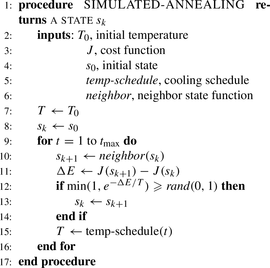
Simulated annealing

The pseudo-code can be explained as follows: Initially we assign to the current temperature T an initial value $T_{0}$ and to the current state $s_{k}$ an initial value $s_{0}$ .

Then, we loop from a starting temperature of $T = 1$ until the maximum defined temperature and at each step:

We assign to the current state a neighbor state by using a neighbor generating function $neighbor (s_{k})$ . We then calculate the change in energy $Δ E$ as the difference between the value in the cost function between the next current state $s_{k + 1}$ and the current state $s_{k}$ . If the change was negative that means that we improved (i.e. minimized) the objective function value with this new state; since $Δ E$ will be negative in such case, $e^{- Δ E / T}$ is greater than 1, and then we assign to the current state the new state. Otherwise, we assign it with probability $e^{- Δ E / T}$ .

At the end of each state, we update the current temperature by using a temperature update function: temp-schedule $(t)$ .

3.2. Adaptive simulated annealing

Adaptive simulated annealing (ASA) is an algorithm proposed by Ingber [10] that is based on simulated annealing. This adaptive version of simulated annealing is based on randomly importance sampling of the parameter space. Ingber [10] remarks that in optimization problems there are different parameters with varying finite ranges and with different annealing-time dependent sensitivities; this serves as a motivation for adaptive simulated annealing where different annealing schedules are held to address the different sensitivities corresponding to each parameter. Keeping individual temperatures for each parameter, re-annealing, and generating new parameters based on the current temperature are some characteristics of ASA.

The motivation of using adaptive simulated annealing for the tuning to PID controllers is precisely the fact that changing the different parameters of the PID controller in the same magnitude can have very different effects in the system output since adaptive simulated annealing maintains temperatures and cooling schedules specifically for each parameter. This technique seems suitable to solve this optimization problem.

Algorithm 2

Adaptive Simulated annealing

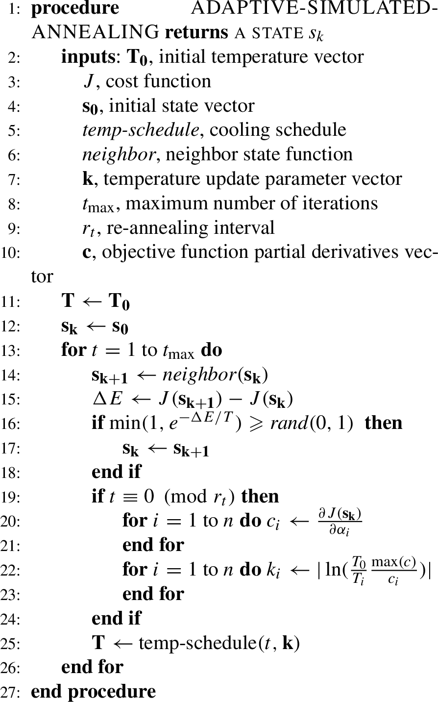
The pseudo-code shown in Algorithm 2 illustrates the differences between Simulated Annealing and Adaptive Simulated Annealing. The main difference is that we keep track of a temperature vector T for each of the n parameters for which the cost function depends instead of a unique scalar temperature T for all parameters. We also keep track of an update parameter vector k, which is later used to update the temperature for each parameter of the cost function.

We perform each step of the Adaptive Simulated Annealing algorithm in the same way as in the simple version; except that, when the number of iterations t is a multiple of the re-annealing interval $r_{t}$ we obtain the partial derivatives of the cost function with respect to each parameter $α_{i}$ , and store them in the vector c. Then we update the temperature update-parameter vector k by assigning to each of its i entries (n in total): $| ln (\frac{T_{0}}{T_{i}} \frac{max (c)}{c_{i}}) |$ ; where $T_{i}$ is the temperature for parameter i and $max (c)$ is the maximum element of vector c.

Finally, at the end of each iteration we update the temperature vector T using the update-parameter vector k and the iteration number t.

3.3. PID controller

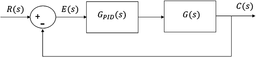
A PID controller can be viewed as an extreme form of a phase lead-lag compensator having one pole in the origin and a second at infinity [2]. The transfer function corresponding to this type of controller is the following: $\begin{matrix} (2) & G (s) = k_{p} + \frac{k_{i}}{s} + k_{d} s \end{matrix}$

Fig. 1.

Block diagram of a closed loop control system with a PID controller. $R (s)$ represents the input of the system (usually a unite step), $E (s)$ the error signal, $C (s)$ the system output, and the $G (s)$ block the system to be controlled.

The PID controller is typically applied to closed loop control systems in a configuration as shown in Fig. 1.

Some of the characteristics that are desirable to improve with the controller regarding the transient response are:

Rise time: The time taken by the system output to go from a low value to a high value (usually above 90% of its final value).

Overshoot: The amplitude of the highest peak with respect to the final value. This parameter is usually measured as a percentage.

Settling time: The time taken by the system output to reach its final value (95% of the final value is the usual measure).

And the feature to be improved concerning the permanent response is:

Steady-state error: The difference between the desired output and the final value of the system after the transient response.

Increasing each of the three gains has different effects on the output of the controlled system [2]:

Increasing $k_{p}$ : Decreases the rise time, increases the overshoot, slightly increases the settling time, decreases the steady-state error and degrades stability.

Increasing $k_{i}$ : Slightly decreases the rise time, increases the overshoot, increases the settling time, largely decreases the steady-state error and degrades stability.

Increasing $k_{d}$ : Slightly decreases the rise time, decreases the overshoot and the settling time, slightly changes the steady-state error and improves stability.

There are many methods for assessing the performance of the output of a system; those methods are useful in constructing a cost function to be used as part of optimization techniques. The following measures serve as single objective cost functions of the performance of a system and are based on the error: Integral of Absolute Error (IAE), Integral of Squared Error (ISE), Integral of Time multiplied by the Absolute Error (ITAE) and Integral of Time multiplied by the Squared Error (ITSE). They are calculated respectively: $\begin{array}{l} (3) & IAE = \int_{0}^{\infty} | e (t) | d t \\ (4) & ISE = \int_{0}^{\infty} e^{2} (t) d t \\ (5) & ITAE = \int_{0}^{\infty} t | e (t) | d t \\ (6) & ITSE = \int_{0}^{\infty} t e^{2} (t) d t \end{array}$ Cost functions that combine different objectives (settling time, overshoot, steady-state error, etc.) are also used as means of multi-objective performance index.

4. Methodology

4.1. Tested systems

Äström et al. in [3] show a series of benchmark systems commonly found in industry and useful to test several PID automatic tuning techniques. The application of tuning rules over known process responses and known plant models have some particular conditions. These conditions make the design methods and tuning rules non-general. This is the main reason of [3] to collect systems which are suitable for testing PID controllers. Four families of those systems are controlled with a PID controller tuned using adaptive simulated annealing:

The first group of plants have multiple equal poles and include first and second order systems. For higher values of α the system has a slow response: $\begin{matrix} (7) & G_{1} (s) = \frac{1}{{(s + 1)}^{α}}, α = 1, 2, 3, 4 \end{matrix}$

The second group of benchmark systems are fourth order systems with poles whose spacing is determined by parameter α [28]. $\begin{array}{l} G_{2} (s) \\ = \frac{1}{(1 + s) (1 + α s) (1 + α^{2} s) (1 + α^{3} s)}, \\ (8) & α = 0.1, 0.2, 0.5 \end{array}$

Third order systems with zeros located at $1 / α$ and three equal poles constitute the third group: $\begin{matrix} (9) & G_{3} (s) = \frac{1 - α s}{{(s + 1)}^{3}}, α = 0.1, 0.2, 0.5, 1, 2 \end{matrix}$

Finally, a group of second order systems with a one second time delay is also tested: $\begin{array}{l} G_{4} (s) = \frac{1}{{(1 + s α)}^{2}} e^{- s}, \\ (10) & α = 0.1, 0.2, 0.5, 1, 2, 5, 10 \end{array}$

4.2. Adaptive simulated annealing

The adaptive version of SA used to tune the PID controllers keeps individual temperatures for each parameter and independent cooling schedule parameters $c_{i}$ . The following components were chosen for the ASA algorithm:

Cooling schedule. The temperature is updated after each step according to the following relation: $\begin{matrix} (11) & T_{i} = T_{0} α^{c_{i}} \end{matrix}$ α was selected to be 0.95. $c_{i}$ and $T_{i}$ represents the cooling schedule parameter and current temperature of parameter i respectively. $T_{0}$ is the initial temperature.

Neighbor generation. For each parameter i a normally distributed random number $λ_{i}$ is generated; neighbor states are then generated using temperature based steps according to the following function: $\begin{matrix} (12) & X_{i} = X_{i} + \frac{T_{i} λ_{i}}{\sqrt{\sum_{k = 1}^{n} λ_{k}}} \end{matrix}$ $X_{i}$ represents the magnitude of parameter i of the search space and $T_{i}$ the temperature of this parameter. Each normally distributed random number is divided by the Euclidean norm of all random variables and then multiplied by the temperature.

Acceptance function: States for which the energy change is positive are accepted with a Boltzmann probability distribution, where T is taken as the maximum temperature of all parameters, and $Δ E$ is the energy change (difference between the last accepted value of the evaluating function and the candidate value of this function): $\begin{matrix} (13) & P (Δ E) = e^{\frac{- Δ E}{T}} \end{matrix}$

Re-annealing: One of the features of adaptive simulated annealing is that after a specific number of steps the temperature is raised again independently for each parameter in the search space. For this experiment, different (as described below) re-annealing intervals were tested, and 175 was found to be the optimal value for those systems. To adjust to the different sensitivities of each parameter, the partial derivatives of the current value of the cost function with respect to each parameter are calculated; then the cooling schedule parameter $c_{i}$ is obtained based on the temperature ratio and a sensitivity ratio between each parameter and the maximum sensitivity calculated. This re-annealing schedule was proposed by Ingber [10]: $\begin{array}{l} (14) & s_{i} = \frac{\partial L}{\partial α_{i}} \\ (15) & c_{i} = | ln (\frac{T_{0}}{T_{i}} \frac{max (s)}{s_{i}}) | \end{array}$

Where L is the current cost function, $α_{i}$ the current value of parameter i, $s_{i}$ the partial derivative of L with respect to $α_{i}$ , $T_{0}$ the initial temperature and $T_{i}$ the current temperature of parameter i.

The optimization algorithm does not consider any bounds for the parameters, and an ideal closed loop control model with no disturbance and no derivative filter is used. Since every application may have very different requirements (for instance, some may prioritize overshoot over settling time), the ITSE cost function was selected to give a general improvement of the system.

Table 1
Resulting cost function (ITSE) value after tuning 20 benchmark systems with simple simulated annealing ( $T_{0} = 75$ °C, constant scale parameter $η = 1$ ) and adaptive simulated annealing ( $T_{0} = 75$ °C, re-annealing after 175 steps). The systems were tuned 30 times with those configurations; and the table shows minimum, maximum and average of the simulations

System Minimum ASA Minimum SA Maximum ASA Maximum SA Average ASA Average SA %Decrease SA->ASA

$G_{1}$ , $α = 1$ 3.28126E−14 3.16306E−10 1.51957E−08 5.38914E−06 2.25162E−09 7.69002E−07 99.71%

$G_{1}$ , $α = 2$ 6.48827E−08 2.29178E−06 4.17797E−07 2.60870E−06 1.47328E−07 2.43776E−06 93.96%

$G_{1}$ , $α = 3$ 0.056711085 0.067037751 0.059249195 0.067040784 0.057609447 0.067039283 14.07%

$G_{1}$ , $α = 4$ 0.806249949 0.809537928 0.811887485 0.835697928 0.80751714 0.818732495 1.37%

$G_{1}$ , $α = 8$ 11.5815742 11.67690248 11.58355417 13.23023769 11.58219552 12.32414603 6.02%

$G_{2}$ , $α = 0.1$ 7.99563E−05 7.99311E−05 8.48778E−05 7.99317E−05 8.07330E−05 7.99313E−05 −1.00%

$G_{2}$ , $α = 0.2$ 0.00153637 0.0012547 0.0020361 0.00153581 0.00162348 0.001481759 −9.56%

$G_{2}$ , $α = 0.5$ 0.06985861 0.070018449 0.071761363 0.071526088 0.070550895 0.070548342 −0.0036%

$G_{3}$ , $α = 0.1$ 0.194227458 0.194396184 0.205095509 0.197156875 0.196737888 0.195337366 −0.72%

$G_{3}$ , $α = 0.2$ 0.31948517 0.319921568 0.32699106 0.332193392 0.320412495 0.324255663 1.19%

$G_{3}$ , $α = 0.5$ 0.799883474 0.811094646 0.800839841 1.006062687 0.800090735 0.873146945 8.37%

$G_{3}$ , $α = 1$ 1.908013685 1.956160971 1.908733605 2.78456457 1.908137842 2.341091507 18.49%

$G_{3}$ , $α = 2$ 5.082382173 5.421020039 5.082693324 20.4012907 5.08250986 10.23233222 50.33%

$G_{4}$ , $α = 0.1$ 0.622449 0.691723394 0.624340079 2.80732558 0.623246649 1.376029046 54.72%

$G_{4}$ , $α = 0.2$ 0.660632617 0.668969013 0.660928656 1.546021432 0.660734712 0.948845043 30.36%

$G_{4}$ , $α = 0.5$ 0.828923492 1.01885133 0.829058133 1.552539677 0.828983917 1.216073093 31.83%

$G_{4}$ , $α = 1$ 0.98936213 0.999201726 0.990111337 1.405266364 0.989490066 1.143018531 13.43%

$G_{4}$ , $α = 2$ 1.136631736 1.144077334 1.138747002 1.247442467 1.137018133 1.183792936 3.95%

$G_{4}$ , $α = 5$ 1.269052208 1.269703702 1.302555452 1.27387108 1.275305511 1.271351474 −0.31%

$G_{4}$ , $α = 10$ 1.320642609 1.320011246 1.428377447 1.320828552 1.351677884 1.320310036 −2.38%

System	Minimum ASA	Minimum SA	Maximum ASA	Maximum SA	Average ASA	Average SA	%Decrease SA->ASA
$G_{1}$ , $α = 1$	3.28126E−14	3.16306E−10	1.51957E−08	5.38914E−06	2.25162E−09	7.69002E−07	99.71%
$G_{1}$ , $α = 2$	6.48827E−08	2.29178E−06	4.17797E−07	2.60870E−06	1.47328E−07	2.43776E−06	93.96%
$G_{1}$ , $α = 3$	0.056711085	0.067037751	0.059249195	0.067040784	0.057609447	0.067039283	14.07%
$G_{1}$ , $α = 4$	0.806249949	0.809537928	0.811887485	0.835697928	0.80751714	0.818732495	1.37%
$G_{1}$ , $α = 8$	11.5815742	11.67690248	11.58355417	13.23023769	11.58219552	12.32414603	6.02%
$G_{2}$ , $α = 0.1$	7.99563E−05	7.99311E−05	8.48778E−05	7.99317E−05	8.07330E−05	7.99313E−05	−1.00%
$G_{2}$ , $α = 0.2$	0.00153637	0.0012547	0.0020361	0.00153581	0.00162348	0.001481759	−9.56%
$G_{2}$ , $α = 0.5$	0.06985861	0.070018449	0.071761363	0.071526088	0.070550895	0.070548342	−0.0036%
$G_{3}$ , $α = 0.1$	0.194227458	0.194396184	0.205095509	0.197156875	0.196737888	0.195337366	−0.72%
$G_{3}$ , $α = 0.2$	0.31948517	0.319921568	0.32699106	0.332193392	0.320412495	0.324255663	1.19%
$G_{3}$ , $α = 0.5$	0.799883474	0.811094646	0.800839841	1.006062687	0.800090735	0.873146945	8.37%
$G_{3}$ , $α = 1$	1.908013685	1.956160971	1.908733605	2.78456457	1.908137842	2.341091507	18.49%
$G_{3}$ , $α = 2$	5.082382173	5.421020039	5.082693324	20.4012907	5.08250986	10.23233222	50.33%
$G_{4}$ , $α = 0.1$	0.622449	0.691723394	0.624340079	2.80732558	0.623246649	1.376029046	54.72%
$G_{4}$ , $α = 0.2$	0.660632617	0.668969013	0.660928656	1.546021432	0.660734712	0.948845043	30.36%
$G_{4}$ , $α = 0.5$	0.828923492	1.01885133	0.829058133	1.552539677	0.828983917	1.216073093	31.83%
$G_{4}$ , $α = 1$	0.98936213	0.999201726	0.990111337	1.405266364	0.989490066	1.143018531	13.43%
$G_{4}$ , $α = 2$	1.136631736	1.144077334	1.138747002	1.247442467	1.137018133	1.183792936	3.95%
$G_{4}$ , $α = 5$	1.269052208	1.269703702	1.302555452	1.27387108	1.275305511	1.271351474	−0.31%
$G_{4}$ , $α = 10$	1.320642609	1.320011246	1.428377447	1.320828552	1.351677884	1.320310036	−2.38%

4.3. ASA and SA benchmark systems tests

The PID tuning for the 20 plants described earlier was tested using the adaptive simulated annealing algorithm. Different initial temperature values: 75°C, 100°C and 125°C were tested with re-annealing interval values of 75, 100, 125, 150 and 175 iterations giving a total of 15 different configurations. The results were compared, and an initial temperature of 75°C in combination with a 175 iterations re-annealing interval provided the best performance overall.

To compare the performance of adaptive simulated annealing with the simple simulated annealing algorithm, i.e. without re-annealing, the next state generation function shown in [31] was used:

The next set of PID values $x^{'}$ is calculated at each iteration as $x^{'} = x + η λ$ .

Where η is the scale parameter and λ a random perturbation with Gaussian distribution.

The scale parameter η is reduced at each iteration ‘k’ proportionally with the same value, α, for which the temperature is decreased: $n (k + 1) = α \cdot n (k)$

This simple simulated annealing version was tested with initial temperatures of 50°, 100°C and 150°C with scale parameter initial values, η, of 1, 25, 50, 100, 125 and 150, making a total of 18 different settings. Low initial temperature values, 50 for instance, showed worst results for the cost function of the $G_{1}$ system with $α = 1, 2, 3, 4$ ; but provided better results for most of the rest of the plants in comparison with the other two initial temperatures tested (which had higher values). This was particularly noticeable for the $G_{3}$ system with $α = 2$ and the $G_{4}$ systems with $α = 0.1, 0.2, 0.5$ . The results for every different system showed different behaviors with distinct initial temperatures and scale parameters: some cost functions decreased while lowering the initial values of those parameters, and some cost functions decreased while increasing those parameters. Therefore, among the 18 combinations tested, one was selected such that it provided the best results in overall for the 20 systems. The temperature scale parameter was set to 0.9. An initial temperature of 50°C along with a scale parameter initial value of $η = 100$ provided the best results.

Finally, this same simulated annealing algorithm was tested, but this time keeping the scale parameter constant; i.e. not decreasing it after each iteration. Initial temperatures of 75°, 100°C and 150°C along with scale parameter values of 1, 2, 5, 10, 20 and 50 were tested as well. As with the simple simulated annealing algorithm, the results varied when increasing or decreasing the parameters: initial temperature and the re-annealing interval. In particular, decreasing the initial temperature worsened the results of all of the $G_{1}$ systems, and decreasing the re-annealing interval improved the results of all the $G_{1}$ systems; while worsening the results for most of the $G_{3}$ and $G_{4}$ systems. Again, one configuration was selected such that it provided the best results in overall for the 20 systems. An initial temperature of 75°C with a scale parameter $η = 1$ showed the best cost function values; and in fact, outperformed the simple simulated annealing version with scale parameter reduction over time.

Both the best adaptive simulated annealing version ( $T_{0} = 75$ °C, re-annealing after 175 steps) and the best simple simulated annealing configuration ( $T_{0} = 75$ °C, constant scale parameter $η = 1$ ) were run 10 times across the 20 different benchmark systems to compare their performance. Table 1 shows the minimum, maximum, and average value of the 10 simulations. The last column of Table 1 shows the percentage decrease in the cost function (ITSE) of the average simple simulated annealing algorithm in relation to that obtained by the adaptive simulated annealing algorithm.

Three systems: $G_{1}$ with $α = 4$ , $G_{3}$ with $α = 2$ and $G_{4}$ with $α = 5$ were tuned using the Ziegler–Nichols sustained oscillations method. The results are shown in Figs 2, 3 and 4.

Fig. 2.

System, $G_{1}$ , $α = 4$ , tuned with Ziegler–Nichols and with adaptive simulated annealing using one arbitrary run. The ASA results show less overshoot, and almost the same settling time and steady state error than Ziegler Nichols. The output $y (t)$ represents the ratio between the actual output and the reference input.

Fig. 3.

System, $G_{3}$ , $α = 2$ , tuned with Ziegler–Nichols and with adaptive simulated annealing using one arbitrary run.The ASA results almost the same settling time, steady state error and overshoot than Ziegler–Nichols; but less total error. The output $y (t)$ represents the ratio between the actual output and the reference input.

Fig. 4.

System, $G_{4}$ , $α = 5$ , tuned with Ziegler–Nichols and with adaptive simulated annealing using one arbitrary run. The ASA results show less overshoot, less settling time and the same steady state error compared to Ziegler–Nichols. The output $y (t)$ represents the ratio between the actual output and the reference input.

4.4. Comparison with other methods

In [26], particle swarm optimization (PSO) is used to find the optimal values of the PID controller of a DC motor. Four different cost functions (ISE, IAE, ITSE, ITAE) are used to find the gains of the PID controller with the PSO algorithm. The three parameters of the controller are limited in the range of 0 to 100.

The following system represents the DC motor model in the Laplace domain: $\begin{matrix} (16) & G (s) = \frac{1}{s^{3} + 9 s^{2} + 23 s + 15} \end{matrix}$

In this section, we use the adaptive simulated annealing algorithm to tune the same controller. The search space is limited in the same range as in [26], and the integration interval used to calculate the four cost functions is set from 0 to 10 seconds. The ASA parameters selected were: Re-annealing interval, 175 iterations; Initial temperature 75°C, and maximum number of iterations 1500. Table 2 shows the result of the comparison. The PID parameters reported in [26] for each objective function were taken and the cost function was calculated under the same conditions reported in that work to compare it with our algorithm.

Table 2
Comparison of best cost function found using a particle swarm optimization approach (PSO) and adaptive simulated annealing (ASA)

Cost function Best cost function value (PSO) Best cost after 100 iterations (ASA) Best cost after 500 iterations (ASA) Best cost after 1000 iterations (ASA) Best cost after 1500 iterations (ASA)

ISE 0.312 0.163 0.1038 0.1034 0.1032

IAE 1.0043 0.3842 0.2627 0.2535 0.2535

ITSE 0.0976 0.0139 0.0135 0.0135 0.0135

ITAE 1.7096 0.2067 0.1187 0.0924 0.0743

Cost function	Best cost function value (PSO)	Best cost after 100 iterations (ASA)	Best cost after 500 iterations (ASA)	Best cost after 1000 iterations (ASA)	Best cost after 1500 iterations (ASA)
ISE	0.312	0.163	0.1038	0.1034	0.1032
IAE	1.0043	0.3842	0.2627	0.2535	0.2535
ITSE	0.0976	0.0139	0.0135	0.0135	0.0135
ITAE	1.7096	0.2067	0.1187	0.0924	0.0743

As mentioned, the four configurations were run for a maximum of 1500 iterations, and the objective function value after 100, 500, 1000 and 1500 iterations is shown in Table 2. The simulations were run on a machine with Intel Core i5 2.4 GHz processor. The running time for each configuration was as follows:

ISE: 70.85 seconds

IAE: 72.57 seconds

ITSE: 69.38 seconds

ITAE: 73.97 seconds

In average the algorithm is running 1500 iterations in 70 seconds, which is roughly equivalent to 21 iterations per second. ASA significantly improved the results obtained with PSO in 100 iterations (roughly 5 seconds according to the calculation above). [26] does not specify the running time used to obtain its results, but mentions a total of 50 PSO iterations being used.

4.5. Systems with constant disturbance

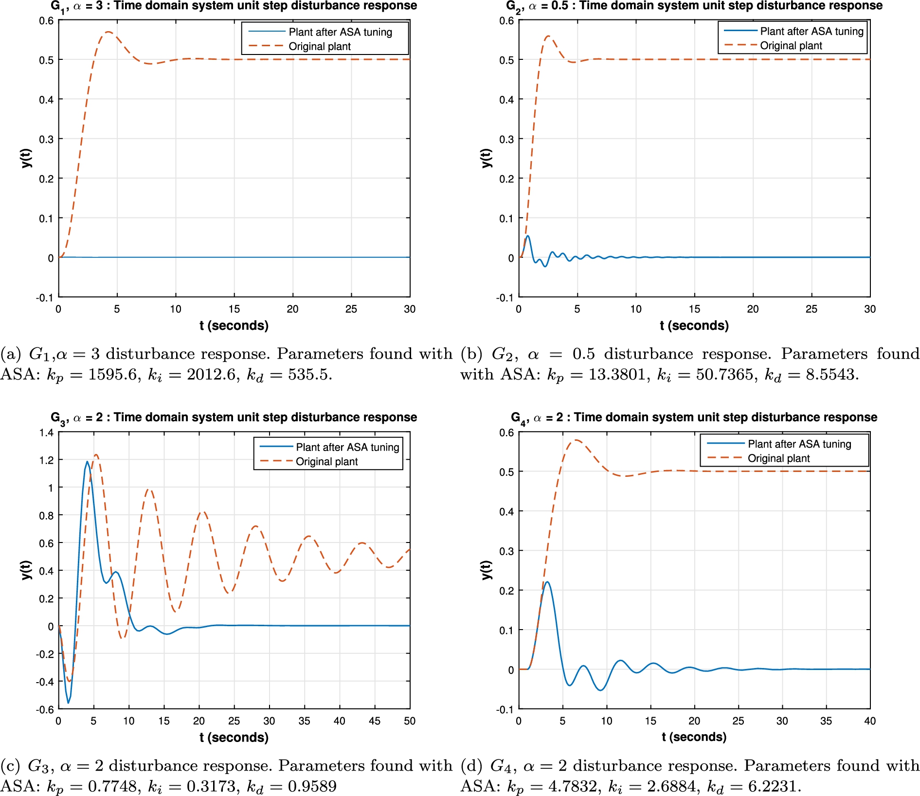
Four systems: $G_{1}$ with $α = 3$ , $G_{2}$ with $α = 0.5$ , $G_{3}$ with $α = 2$ and $G_{4}$ with $α = 2$ were set with a unit step disturbance (nominal input) and with a zero input reference. A PID controller was tuned with adaptive simulated annealing to correct the error due to the constant disturbance and to take the output of the system to zero. Figure 5 shows the output of such systems with the PID parameters found for each one. The three parameters were obtained by using the same configuration that was used to tune the PID controllers for the systems in Table 1.

Fig. 5.

One system of each of the four families of plants discussed earlier. Each system was set with an input reference of 0 and with a unit step disturbance. The PID was tuned with ASA to correct the error due to this disturbance. When analyzing the disturbance rejection of a control system, a reference input (set point) of zero is typically used to limit the analysis to just disturbance rejection.

Figure 6 shows the configuration of a system with a PID controller to correct the error due to a disturbance signal $D (s)$ and with a reference input signal $R (s)$ .

5. Results

This section reports the results generated after running ASA and comparing it against particle swarm optimization. The reason to choose PSO for comparison is based on the interest of comparing ASA against another optimization-based approach, and the fact that PSO reported interesting results according to [26]. The results (minimum, maximum, average cost function value) after running the simulations with 30 repetitions and for the 20 different benchmark systems are shown in Tables 1, 3–5. For each system we report the three gains and the respective system characteristics after tuning with ASA (percentage overshoot, steady-state error, and settling time). Three of those systems were selected for comparison with the Ziegler–Nichols algorithm by creating a plot of the system after being tuned by both methods. To compare ASA with PSO, a DC motor system representation was tuned using both methods, and the results are described as well. Finally, plots of four systems under constant disturbance are shown before and after PID tuning with the technique described in this paper.

Fig. 6.

Block diagram of a closed loop control system with a PID controller and disturbance. 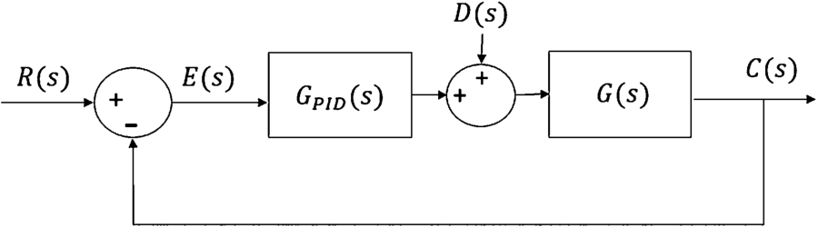$R (s)$ represents the input of the system (zero in this case), $E (s)$ the error signal, $C (s)$ the system output, the $G (s)$ block the system to be controlled and $D (s)$ the disturbance signal.

Table 3

Resulting standard deviation of the cost function (ITSE) value after tuning 20 benchmark systems with simple simulated annealing ( $T_{0} = 75$ °C, constant scale parameter $η = 1$ ) and adaptive simulated annealing ( $T_{0} = 75$ °C, re-annealing after 175 steps). The systems were tuned 30 times with those configurations, and the table shows the standard deviation of all the simulations

System	Standard Deviation ASA	Standard Deviation SA
$G_{1}$ , $α = 1$	3.50E−09	1.33E−06
$G_{1}$ , $α = 2$	7.06E−08	7.70E−08
$G_{1}$ , $α = 3$	5.15E−04	8.43E−07
$G_{1}$ , $α = 4$	1.44E−03	6.01E−03
$G_{1}$ , $α = 8$	4.44E−04	4.64E−01
$G_{2}$ , $α = 0.1$	9.78E−07	1.27E−10
$G_{2}$ , $α = 0.2$	1.13E−04	9.82E−05
$G_{2}$ , $α = 0.5$	6.24E−04	3.27E−04
$G_{3}$ , $α = 0.1$	3.11E−03	6.58E−04
$G_{3}$ , $α = 0.2$	1.77E−03	2.59E−03
$G_{3}$ , $α = 0.5$	2.35E−04	3.92E−02
$G_{3}$ , $α = 1$	1.85E−04	0.21160
$G_{3}$ , $α = 2$	8.56E−05	3.5226
$G_{4}$ , $α = 0.1$	4.34E−04	0.4996
$G_{4}$ , $α = 0.2$	7.34E−05	0.21055
$G_{4}$ , $α = 0.5$	3.69E−05	0.1314
$G_{4}$ , $α = 1$	1.35E−04	9.38E−02
$G_{4}$ , $α = 2$	4.21E−04	2.38E−02
$G_{4}$ , $α = 5$	7.44E−03	1.07E−03
$G_{4}$ , $α = 10$	0.0258	1.86E−04

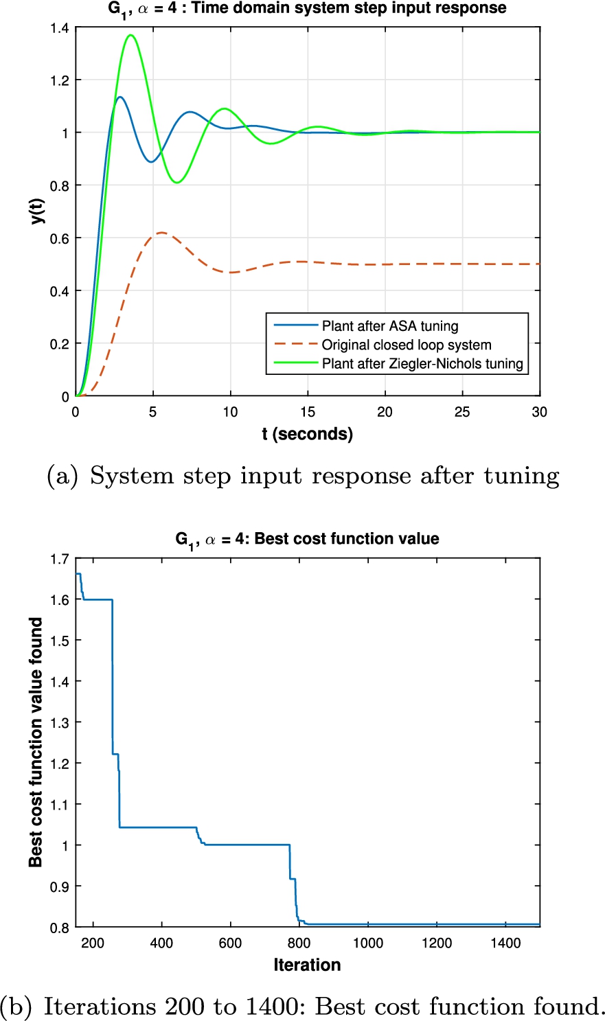
To illustrate the ASA algorithm performance graphically, three different systems; $G_{1}$ with $α = 4$ , $G_{3}$ with $α = 2$ and $G_{4}$ with $α = 5$ ; were tuned using the Ziegler–Nichols method; and after obtaining the three gains, the output of the system was plotted against the same obtained by tuning it with adaptive simulated annealing. The Ziegler–Nichols method can be used to tune most systems, but we just selected three of the total 20 to show the results using this widely used algorithm (Ziegler–Nichols) and ASA. Figures 2, 3 and 4 show the system step input response along with a plot of the best overall cost function found at each step. For the $G_{1}$ with $α = 4$ case, our proposed algorithm improved slightly the settling time and significantly the percentage overshoot of the system. The ASA algorithm just required 800 iterations, as shown in Fig. 2(b), to nearly find the final parameters. For the $G_{3}$ with $α = 2$ system, the ASA approach improved the settling time requiring around 1000 iterations to come close to the final parameters (those with the best cost function found by ASA); those results are shown in Fig. 3. Finally, after using ASA and Ziegler–Nichols tuning $G_{4}$ with $α = 5$ , the former greatly improved both the overshoot and settling time in contrast to the latter, as shown in Fig. 3, just requiring 1000 iterations to get very close to the optimal values found by ASA.

Table 4

Resulting average characteristics and PID parameters of 20 different benchmark system after being tuned with adaptive simulated annealing ( $T_{0} = 75$ °C, re-annealing after 175 steps). The systems were tuned 30 times with those configurations, and the table shows the average of the 30 results

System	Average percentage overshoot	Average abs. value of steady-state error	Average settling time (seconds)	Average $k_{p}$	Average $k_{i}$	Average $k_{d}$
$G_{1}$ , $α = 1$	406.860%	3.55E−15	0.001716	177.382	158.082	−1.005
$G_{1}$ , $α = 2$	0.003%	3.33E−17	0.004163	1551.193	803.636	1012.011
$G_{1}$ , $α = 3$	87.987%	3.87E−05	2.60477	46.6663	551.207	1479.417
$G_{1}$ , $α = 4$	14.116%	−9.10E−09	12.0339	2.345	0.933	4.201
$G_{1}$ , $α = 8$	11.419%	1.50E−04	24.94153	0.979	0.218	2.759
$G_{2}$ , $α = 0.1$	29.636%	1.67E−16	0.09581	123.157	125.494	16.209
$G_{2}$ , $α = 0.2$	25.488%	1.07E−16	0.46656	25.928	30.705	6.986
$G_{2}$ , $α = 0.5$	16.606%	7.03E−17	3.94392	4.216	3.234	3.014
$G_{3}$ , $α = 0.1$	19.646%	4.23E−11	6.977	4.334	2.193	6.251
$G_{3}$ , $α = 0.2$	15.422%	−2.38E−11	7.9128	3.093	1.449	4.094
$G_{3}$ , $α = 0.5$	11.083%	1.84E−11	7.8852	1.841	0.810	2.226
$G_{3}$ , $α = 1$	6.769%	−1.74E−11	9.2084	1.166	0.493	1.332
$G_{3}$ , $α = 2$	6.826%	8.48E−10	10.7682	0.703	0.284	0.769
$G_{4}$ , $α = 0.1$	21.047%	6.59E−14	5.7866	0.531	0.870	0.127
$G_{4}$ , $α = 0.2$	17.174%	3.55E−13	4.8688	0.623	0.881	0.237
$G_{4}$ , $α = 0.5$	10.475%	−8.35E−13	5.99009	0.902	0.792	0.523
$G_{4}$ , $α = 1$	10.686%	−1.33E−12	7.42301	1.414	0.723	1.230
$G_{4}$ , $α = 2$	11.864%	−9.01E−11	8.6794	2.485	0.669	3.581
$G_{4}$ , $α = 5$	14.116%	1.90E−06	7.4767	5.859	0.635	18.328
$G_{4}$ , $α = 10$	16.188%	−8.52E−05	7.7835	12.294	0.632	68.131

Table 5

Resulting minimum characteristics and PID parameters of 20 different benchmark system after being tuned with adaptive simulated annealing ( $T_{0} = 75$ °C, re-annealing after 175 steps). The systems were tuned 30 times with those configurations, and the table shows the minimum of the 30 results for each system

System	Minimum percentage overshoot	Minimum abs. value of steady-state error	Minimum settling time (seconds)	Minimum $k_{p}$	Minimum $k_{i}$	Minimum $k_{d}$
$G_{1}$ , $α = 1$	8.8818E−14%	−7.11E−15	0.001715	−1579.614	−1445.306	−1.508
$G_{1}$ , $α = 2$	1.8969E−04%	−2.22E−16	0.003414	1021.561	533.561	729.357
$G_{1}$ , $α = 3$	82.500%	−6.39E−04	2.54757	29.743	203.116	629.518
$G_{1}$ , $α = 4$	12.956%	−1.81E−08	9.33244	2.306	0.879	3.898
$G_{1}$ , $α = 8$	10.800%	−1.67E−04	24.8927	0.973	0.216	2.737
$G_{2}$ , $α = 0.1$	24.789%	−4.44E−16	0.069532	104.192	86.603	13.419
$G_{2}$ , $α = 0.2$	18.036%	−8.88E−16	0.3076	19.679	16.601	5.361
$G_{2}$ , $α = 0.5$	13.539%	−1.78E−15	2.64418	4.003	2.776	2.691
$G_{3}$ , $α = 0.1$	14.907%	−6.05E−11	6.33833	3.972	1.818	5.361
$G_{3}$ , $α = 0.2$	13.393%	−6.75E−11	7.6274	2.987	1.347	3.757
$G_{3}$ , $α = 0.5$	9.846%	−9.86E−12	7.466	1.810	0.794	2.190
$G_{3}$ , $α = 1$	6.327%	−4.51E−11	9.1117	1.162	0.487	1.313
$G_{3}$ , $α = 2$	6.604%	7.41E−10	10.70126	0.700	0.283	0.766
$G_{4}$ , $α = 0.1$	17.569%	−4.57E−12	5.39284	0.513	0.854	0.124
$G_{4}$ , $α = 0.2$	16.255%	2.30E−13	4.6374	0.618	0.870	0.233
$G_{4}$ , $α = 0.5$	10.056%	−1.02E−12	5.9823	0.895	0.786	0.519
$G_{4}$ , $α = 1$	10.125%	−3.72E−12	7.39401	1.403	0.712	1.217
$G_{4}$ , $α = 2$	10.960%	−6.77E−10	8.37078	2.453	0.644	3.509
$G_{4}$ , $α = 5$	9.719%	−6.13E−06	7.16988	5.483	0.585	16.268
$G_{4}$ , $α = 10$	7.184%	−2.64E−04	5.6130	10.128	0.482	59.281

Table 6 shows the results of running each system for both ASA and SA in a computer with an Intel Core i5-6300HQ CPU at 2.3 GHz CPU. In general, SA can run slightly more iterations per second than ASA given the fact that in the ASA algorithm, in the re-annealing interval the gradient for each parameter has to be calculated.

Table 6

The table shows the running time for a single run of each system using both ASA and SA. The table also shows the number of iterations each algorithm run, and the iterations per second for each algorithm and system. As in the previous experiments, the algorithm was set to run for 9000 iterations stopping the algorithm if no improvement was made after 1500 iterations

System	ASA Running time (seconds)	SA Running time (seconds)	Number of iterations ASA	Number of iterations SA	Iterations per second ASA	Iterations per second SA
$G_{1}$ , $α = 1$	319.582	306.090	9000	9000	28.162	29.403
$G_{1}$ , $α = 2$	145.265	111.754	3779	2809	26.014	25.136
$G_{1}$ , $α = 3$	255.265	244.525	9000	9000	35.257	36.806
$G_{1}$ , $α = 4$	240.155	225.697	9000	9000	37.476	39.877
$G_{1}$ , $α = 8$	240.166	226.949	9000	9000	37.474	39.656
$G_{2}$ , $α = 0.1$	1616.406	346.521	9000	9000	5.568	25.972
$G_{2}$ , $α = 0.2$	286.405	263.584	9000	9000	31.424	34.145
$G_{2}$ , $α = 0.5$	276.815	264.458	9000	9000	32.513	34.032
$G_{3}$ , $α = 0.1$	254.976	230.426	9000	9000	35.297	39.058
$G_{3}$ , $α = 0.2$	265.259	228.476	9000	9000	33.929	39.391
$G_{3}$ , $α = 0.5$	270.337	267.995	9000	9000	33.292	33.583
$G_{3}$ , $α = 1$	262.206	238.182	9000	9000	34.324	37.786
$G_{3}$ , $α = 2$	273.076	221.663	9000	9000	32.958	40.602
$G_{4}$ , $α = 0.1$	458.638	443.777	9000	9000	19.623	20.280
$G_{4}$ , $α = 0.2$	408.957	381.264	9000	9000	22.007	23.606
$G_{4}$ , $α = 0.5$	336.279	310.643	9000	9000	26.764	28.972
$G_{4}$ , $α = 1$	339.227	301.379	9000	9000	26.531	29.863
$G_{4}$ , $α = 2$	379.087	289.279	9000	9000	23.741	31.112
$G_{4}$ , $α = 5$	340.711	278.141	9000	9000	26.415	32.358
$G_{4}$ , $α = 10$	323.470	310.834	9000	9000	27.823	28.954

Table 1 shows the minimum, maximum, and average cost function (ITSE) values for the 20 benchmark systems after SA and ASA tuning. The last column shows the percentage decrease in the cost function of the average simple simulated annealing algorithm in relation to that obtained by the adaptive simulated annealing algorithm. The results show that for 14 of the 20 system tested there was a decrease in the cost function when using ASA with respect to SA; and for the remaining 5 systems, where the average cost function was greater in ASA, the percentage increase of using ASA with respect to SA was lower than 10% for all five cases.

The desired system characteristics are something that varies among different applications. Some systems where speed is the major factor prefer to improve the settling time while sacrificing percentage overshoot, and in other applications where avoiding peaks is the priority, percentage overshoot can be improved at the expense of settling time for instance. Decreasing the percentage overshoot, the steady state error, and the settling time have the effect of decreasing the objective function ITSE, so this is why all of the systems were tested only considering the value function to provide greater generality.

The average, minimum and maximum values of the system characteristics and their corresponding $k_{p}$ , $k_{i}$ and $k_{d}$ gains after ASA tuning are shown in Table 4, Table 5 and Table 7 respectively. Those results demonstrate that the algorithm produced varied results regarding the gains and system characteristics while keeping a similar cost function value. For instance, for $G_{1}$ with $α = 1$ , the minimum percentage overshoot was 8.8818E−14%, and the maximum percentage overshoot was 2971.307% ; however, both the minimum and maximum cost function were below 1.0E−5. Table 3 shows the standard deviation obtained for each system after running 30 times the simulation. 8 of the 20 results (rows starting at $G_{3}$ with $α = 0.5$ and ending in $G_{4}$ with $α = 5$ ) in this table show a much lower standard deviation for the Adaptive Simulated Annealing simulations, suggesting more consistent results for those configurations with ASA.

Table 7

Resulting maximum characteristics and PID parameters of 20 different benchmark system after being tuned with adaptive simulated annealing ( $T_{0} = 75$ °C, re-annealing after 175 steps). The systems were tuned 30 times with those configurations, and the table shows the maximum of the 30 results for each system

System	Maximum percentage overshoot	Maximum abs. value of steady-state error	Maximum settling time (seconds)	Maximum $k_{p}$	Maximum $k_{i}$	Maximum $k_{d}$
$G_{1}$ , $α = 1$	2971.307%	1.14E−13	0.00173	1686.658	1487.652	−0.570
$G_{1}$ , $α = 2$	0.00593%	4.44E−16	0.005526	1951.671	955.449	1209.862
$G_{1}$ , $α = 3$	90.719%	6.39E−04	2.6648	58.175	904.424	2379.001
$G_{1}$ , $α = 4$	15.862%	9.58E−09	12.2243	2.428	0.995	4.493
$G_{1}$ , $α = 8$	11.866%	−1.33E−04	24.9801	0.983	0.219	2.785
$G_{2}$ , $α = 0.1$	34.652%	6.66E−16	0.115417	137.614	228.309	19.515
$G_{2}$ , $α = 0.2$	37.559%	8.88E−16	0.930472	37.712	105.120	9.917
$G_{2}$ , $α = 0.5$	19.814%	1.78E−15	4.22339	4.570	3.921	3.336
$G_{3}$ , $α = 0.1$	26.351%	4.66E−10	7.5567	5.000	2.769	7.294
$G_{3}$ , $α = 0.2$	20.711%	2.25E−11	8.09092	3.363	1.705	4.366
$G_{3}$ , $α = 0.5$	11.691%	4.53E−11	9.27546	1.856	0.826	2.254
$G_{3}$ , $α = 1$	7.273%	7.43E−11	9.3598	1.172	0.500	1.341
$G_{3}$ , $α = 2$	7.074%	1.02E−09	10.85137	0.705	0.286	0.772
$G_{4}$ , $α = 0.1$	24.429%	1.94E−12	6.4242	0.548	0.890	0.131
$G_{4}$ , $α = 0.2$	18.433%	6.44E−13	5.35986	0.629	0.893	0.243
$G_{4}$ , $α = 0.5$	11.078%	−4.23E−13	6.0001	0.906	0.800	0.528
$G_{4}$ , $α = 1$	11.538%	6.25E−13	7.4528	1.424	0.739	1.259
$G_{4}$ , $α = 2$	12.566%	6.02E−10	8.84518	2.514	0.683	3.642
$G_{4}$ , $α = 5$	18.770%	7.52E−06	7.82972	6.188	0.690	19.914
$G_{4}$ , $α = 10$	26.904%	8.03E−05	10.315	14.827	0.816	78.094

Table 2 shows the optimal values for each cost function found by using ASA after 100, 500, 1000 and 1500 iterations along with the cost function value obtained by using PSO. Table 8 shows the PID values found for each cost function, the resulting overshoot and the settling time. After just 100 iterations, ASA obtained a better value than PSO for the four cost functions used to tune the DC motor system representation. The settling time was below 4 seconds and the percentage overshoot below 15% for all the cases (4 different cost functions).

Table 8

Proportional, derivative and integral gains of the PID controllers obtained after tuning the DC motor using adaptive simulated annealing for the four cost functions described earlier

Cost function	$k_{p}$	$k_{i}$	$k_{d}$	Overshoot	Settling time (seconds)
ISE	99.6727	99.998	99.5863	12.83%	3.997
IAE	99.9671	75.6893	47.7092	6.23%	1.2708
ITSE	99.9273	90.4924	63.8036	7.29%	1.2062
ITAE	99.1446	66.3086	33.1841	8.59%	1.4186

As mentioned earlier, $G_{1}$ , $α = 3$ ; $G_{2}$ , $α = 0.5$ ; $G_{3}$ , $α = 2$ and $G_{4}$ , $α = 2$ were selected to test the tuning algorithm with a constant disturbance and a zero reference input. In the four cases, ASA tuning effectively rejected the disturbance, as shown in Figs 5(a), (b), (c) and (d). For the first two systems, the output reached zero in less than five seconds while for the last two systems this happened in less than 20 seconds.

In [27], the authors report the design of a PID controller for an air heater temperature control system. The approach is based on the application of PSO. The authors perform simulations and according to them, the simulation results are achieved that the PSO optimized PID controller is able to improve the performance when compared with the Ziegler–Nichols as well as with GA in the perspectives of transient responses.

6. Conclusions

The tests showed that the best adaptive simulated annealing version outperformed the best simple simulated annealing version. Particularly, out of the 20 benchmark systems tested, for 14 of them the average smallest cost function was achieved through adaptive simulated annealing. For 10 of those systems, the percentage decrease with respect to the average simple simulated annealing cost function was greater than 5%, and only in one benchmark system this percentage decrease was greater than 5%. This best ASA version was able to obtain a smaller cost function than that obtained by PSO in less than 100 iterations for the four different cost functions described earlier. The tests performed in four of the benchmark systems demonstrated that ASA can also be effectively used to tune PID controllers for plants with constant disturbance.

The desired characteristics of the controlled systems were improved with respect to the original system (no control): overshoot, settling time and steady state error. The comparisons with the Ziegler–Nichols tuning method and with simple simulated annealing show that the idea of adapting the algorithm to each of the three parameters, which have very different effects on the system, proved to be fruitful.

References

Allaoua ,

Gasbaoui and

Mebarki , Setting up PID DC motor speed control alteration parameters using particle swarm optimization strategy, Leonardo Electronic Journal of Practices and Technologies 14 (2009), 19–32.

K.H.

Ang ,

Chong and

Li , PID control system analysis, design, and technology, IEEE Transactions on Control Systems Technology 13(4) (2005), 559–576. doi:10.1109/TCST.2005.847331.

K.J.

Åström and

Hägglund , Benchmark systems for PID control. Digital Control – Past, Present, and Future of PID Control 33(4) (2000), 165–166.

Bertsimas and

Tsitsiklis , Simulated annealing, Statistical Science 8(1) (1993), 10–14. doi:10.1214/ss/1177011077.

Chen ,

Ren and

Fan , Particle swarm optimization with adaptive mutation and its application research in tuning of PID parameters, in: 1st International Symposium on Systems and Control in Aerospace and Astronautics, IEEE, 2006.

Z.-L.

Gaing , A particle swarm optimization approach for optimum design of PID controller in AVR system, IEEE Trans. Energy Conversion 19(2) (2004), 384–391. doi:10.1109/TEC.2003.821821.

GirirajKumar ,

Rakesh and

Anantharaman , Design of controller using simulated annealing for a real time process, International Journal of Computer Applications 6(2) (2010), 20–25. doi:10.5120/1053-1368.

Haber ,

Haber-Haber ,

del Toro and

Alique , Using simulated annealing for optimal tuning of a PID controller for time-delay systems. An application to a high-performance drilling process, in: Computational and Ambient Intelligence, 2007, pp. 1155–1162. doi:10.1007/978-3-540-73007-1_140.

Herrero ,

Blasco ,

Martinez and

Salcedo , Optimal PID tuning with genetic algorithms for non-linear process models, in: 15th Triennial World Congress, Barcelona, Spain, Citeseer, 2002.

10.

Ingber

et al., Adaptive simulated annealing (ASA): Lessons learned, Control and Cybernetics 25 (1996), 33–54.

11.

Jones and

de Moura Oliveira , Genetic auto-tuning of PID controllers, in: First International Conference on Genetic Algorithms in Engineering Systems: Innovations and Applications, IET, 1995, pp. 141–145.

12.

Shojaee ,

H.G.

Shakouri and

M.B.

Taghadosi , Importance of the initial conditions and the time schedule in the simulated annealing, in: Simulated Annealing, Theory with Applications, 2010, pp. 217–234.

13.

Kennedy , Particle swarm optimization, in: Encyclopedia of Machine Learning, Springer, 2010, pp. 760–766.

14.

Kirkpatrick ,

C.D.

Gelatt ,

M.P.

Vecchi et al., Optimization by simulated annealing, Science 220(4598) (1983), 671–680. doi:10.1126/science.220.4598.671.

15.

Kishnani ,

Pareek and

Gupta , Optimal tuning of PID controller using meta heuristic approach, International Journal of Electronic and Electrical Engineering 7 (2014), 171–176.

16.

Kumar and

N.K.

Nair , Multiobjective robust PID controller design for various industrial processes, AI Communications 28(3) (2015), 567–578. doi:10.3233/AIC-140639.

17.

Lu ,

Yang ,

Peng ,

Wan ,

Han and

Ma , Self-tuning PID control scheme with swarm intelligence based on support vector machine, in: IEEE International Conference on Mechatronics and Automation (ICMA), IEEE, 2014, pp. 1554–1558.

18.

W.L.

Luyben , Process Modeling, Simulation and Control for Chemical Engineers, 2nd edn, McGraw-Hill Higher Education, 1989.

19.

Mitchell , An Introduction to Genetic Algorithms, MIT Press, 1998.

20.

Moness and

A.M.

Moustafa , Tuning a digital multivariable controller for a lab-scale helicopter system via simulated annealing and evolutionary algorithms, Transactions of the Institute of Measurement and Control 37(10) (2015), 1254–1273. doi:10.1177/0142331214560806.

21.

Ogata , Modern Control Engineering, 5th edn, Prentice Hall, 2009.

22.

D.S.

Pereira and

J.O.

Pinto , Genetic algorithm based system identification and PID tuning for optimum adaptive control, in: Proceedings, International Conference on Advanced Intelligent Mechatronics, IEEE, 2005, pp. 801–806.

23.

Porter and

Jones , Genetic tuning of digital PID controllers, Electronics Letters 28(9) (1992), 843–844. doi:10.1049/el:19920533.

24.

Reynoso-Meza ,

Carrillo-Ahumada ,

Boada and

Picó , PID controller tuning for unstable processes using a multi-objective optimisation design procedure, IFAC-PapersOnLine 49(7) (2016), 284–289. doi:10.1016/j.ifacol.2016.07.287.

25.

R.A.

Rutenbar , Simulated annealing algorithms: An overview, in: IEEE Circuits and Devices Magazine, 1989, pp. 19–26.

26.

M.I.

Solihin ,

L.F.

Tack and

M.L.

Kean , Tuning of PID controller using particle swarm optimization (PSO), International Journal on Advanced Science, Engineering and Information Technology 1(4) (2011), 458–461. doi:10.18517/ijaseit.1.4.93.

27.

Sungthong and

Assawinchaichote , Particle swam optimization based optimal PID parameters for air heater temperature control system, Procedia Computer Science 86 (2016), 108–111. doi:10.1016/j.procs.2016.05.027.

28.

Thammarat ,

Sukserm and

Puangdownreong , Design of PID controllers via genetic algorithm for benchmark systems, in: Proceeding of the 4th Annual International Conference on Electrical Engineering/Electronics Computer, Telecommunications and Information Technology, 2007, pp. 221–224.

29.

Tharmalingam and

Raahemifar , Strategic iniitialization of a hybrid particle swarm optimization-simulated annealing algorithm (HPSOSA) for PID controller design for a nonlinear system, in: Electrical & Computer Engineering (CCECE), 2012 25th IEEE Canadian Conference on, IEEE, 2012, pp. 1–4.

30.

Wang and

Kwok , Optimal design of PID process controllers based on genetic algorithms, Control Eng. Pract. 2(4) (1994), 641–648. doi:10.1016/0967-0661(94)90008-6.

31.

Yachen and

Yueming , On PID controllers based on simulated annealing algorithm, in: 27th Chinese Control Conference, IEEE, 2008, pp. 225–228. doi:10.1109/CHICC.2008.4605420.

32.

J.G.

Ziegler and

N.B.

Nichols , Optimum settings for automatic controllers, Trans. ASME 64(11) (1942).