Towards backbone computing: A Greedy-Whitening based approach

Abstract

Backbone is the set of literals that are true in all formula’s models. Computing a part of backbone efficiently could guide the following searching in SAT solving and accelerate the process, which is widely used in fault localization, product configuration, and formula simplification. Specifically, iterative SAT testings among literals are the most time consumer in backbone computing. We propose a Greedy-Whitening based algorithm in order to accelerate backbone computing. On the one hand, we try to reduce the number of SAT testings as many as possible. On the other hand, we make every inventible SAT testing more efficient. The proposed approach consists of three steps. The first step is a Greedy-based algorithm which computes an under-approximation of non-backbone ${\overline{BL}}_{⇂} (Φ)$ . Backbone computing is accelerated since SAT testings of literals in ${\overline{BL}}_{⇂} (Φ)$ are saved. The second step is a Whitening-based algorithm with two heuristic strategies which computes an approximation set of backbone $\hat{BL} (Φ)$ . Backbone computing is accelerated since more backbone are found at an early stage of the computing by testing the literals in $\hat{BL} (Φ)$ first, which makes every individual SAT testing more efficient. The exact backbone is computed in the third step which applies iterative backbone testing on the approximations. We implemented our approach in a tool Bone and conducted experiments on instances from Industrial tracks of SAT Competitions between 2002 and 2016. Empirical results show that Bone is more efficient in industrial and crafted formulas.

Keywords

Backbone satisfiability approximation greedy whitening

1. Introduction

The backbone of a satisfiable formula is a set of literals that are true in all formula’s models, which plays an important role for understanding the hardness of problems in computation complexity. For satisfiability problem [20], backbone provides a good explanation for the apparent inevitably high cost of heuristic search near the phase boundary.

The identification of backbone has many practical applications [14,17,18,23]. The seminal work of using backbone information in solving SAT formulas is introduced in [5]. Dubois and Dequen designed an efficient DPL-type algorithms for solving hard random k-SAT formulas, more specifically, 3-SAT formulas. They chose backbone variables as branch nodes for the tree developed by a DPL-type procedure. Experiments show that the performance of handling unsatisfiable hard 3-SAT formulas had improved significantly. Backbone improves the performance of the random SAT solver like WalkSAT [22] by making biased moves in a local search [21,25]. In addition, backbone can significantly contributes to the Lin-Kernighan local search algorithms for Travel Salesman Problem [24]. Another recent successful application of backbone is post-silicon fault localisation in integrated circuits [26,27].

However, deciding whether a literal is a backbone literal is co-NP complete [7,10]. Many heuristic approaches were proposed to compute backbone, such as model enumeration, iterative SAT-testing and filtering with modern SAT solvers. Marques-Silva et al. conducted an experimental evaluation by integration existing algorithms with optimisations in a modern SAT solver and showed that backbone computation for large practical formulae is feasible [11,12,15].

In this paper, we propose a novel Greedy-Whitening based approach Bone for computing backbones. Greedy Algorithm is widely used in optimization application. We use Greedy Algorithm to greedily select the best fit variables at each iteration. Whitening Algorithm [4,8,9] was used to find essential nodes that cannot be colored as white without changing the color of their adjacent nodes in a k-coloring problem, based on a given coloring plan. Getting a new coloring plan is intuitively easier with known essential nodes.

There are two types of backbone computing algorithms, upper bound estimations and literals testing. The upper bound estimations tries to find the exact backbone by removing (adding) literals from the set of all literals (an empty literal set) of the given formula. The literals testing tests the satisfiability of the original formula together with the given literals (as assumptions), backbone information is extracted from the SAT solving process.

The insight of our Greedy-Whitening approach has two-folds: 1) we present a fast procedure to compute an under-approximation set of non-backbone based on Greedy Algorithm, which prunes the search space during the computation of backbone; 2) we also computes an approximation of backbone in polynomial time based on Whitening Algorithm, and the elements in this set have high possibility to be backbone literals which help us to compute the exact backbone using SAT solvers.

We implemented our approach in a tool Bone and evaluated this tool with empirical experiments. We tested 784 industrial and crafted formulae with time limits, the formulae are selected from SAT competitions during 2002 to 2016.1

¹
http://www.satcompetition.org/

9 more formulas are solved by Bone. For selected industrial formulas, Bone solved 34 from satisfiable industrial formulae in 3600 seconds and reduces 21% total solving time comparing to Minibones. Especially, for group mrpp, Bone reduces 38% solving time.

2. Preliminaries

We fix a finite set $X$ of Boolean variables. A literal l is either a Boolean variable $x \in X$ or its negation $\neg x$ . The negation of a literal $\neg x$ is x, i.e., $\neg \neg x = x$ . A clause ϕ is a disjunction of literals $⋁_{i = 1}^{n} l_{i}$ , which may be regarded as the set of literals ${l_{i} ∣ 1 ⩽ i ⩽ n}$ . W.l.o.g., we assume that for every clause ϕ, if $l \in ϕ$ , then $\neg l \notin ϕ$ .

A formula Φ over $X$ is a Boolean combination of variables $X$ . We assume that formulae are given in conjunctive normal form (CNF), namely each formula Φ is a conjunction of clauses $⋀_{i = 1}^{n} ϕ_{i}$ which may be regarded as a set of clauses ${ϕ_{i} ∣ 1 ⩽ i ⩽ n}$ . Given a formula Φ, let $var (Φ)$ (resp. $L (Φ)$ and $cls (Φ)$ ) denote the set of variables (resp. literals and clauses) used in Φ. The size $| Φ |$ of Φ is the number of literals of Φ. We use $‖ Φ ‖$ to denote $\sum_{ϕ \in Φ} | ϕ |$ , and $\neg L (Φ)$ to denote the set ${\neg l ∣ l \in L (Φ)}$ .

Given a formula Φ and a literal $l \in L (Φ)$ , let $Φ_{l} \subseteq Φ$ be the set of clauses ${ϕ \in Φ ∣ l \in ϕ}$ . Given two different variables $x_{1}, x_{2} \in var (Φ)$ , $x_{1}$ and $x_{2}$ are adjacent variables iff there exists a clause $ϕ \in Φ$ such that $(x_{1} \in ϕ) \land (x_{2} \in ϕ)$ .

An assignment is a function $λ : X \to {0, 1}$ , where 1 (resp. 0) denotes true (resp. false). Given an assignment λ and a literal l that is x or $\neg x$ , let $λ [\neg l]$ be the assignment which is equal to λ except for $λ [\neg l] (x) = \neg λ (x)$ . Given a set of variables $x = {x_{1}, \dots, x_{n}}$ , let $λ [\neg L]$ denote the assignment $λ [\neg x_{1}] .. . [\neg x_{n}]$ .

An assignment λ satisfies a formula Φ, denoted by $λ ⊧ Φ$ , iff assigning $λ (x)$ to x for $x \in var (Φ)$ makes Φ true.

Definition 1 (Backbone).

Given a satisfiable formula Φ, a literal l is a backbone literal of Φ iff for all assignments λ such that $λ ⊧ Φ$ , $λ (l) = 1$ . The backbone $BL (Φ)$ of Φ is the set of backbone literals of Φ.

It is known that the backbone $BL (Φ)$ for each formula Φ is unique [5]. The backbone of an unsatisfiable formula can be defined as an empty set. Therefore, in this work, we focus on satisfiable formulae. We will use $\overline{BL} (Φ)$ to denote the set $L (Φ) ∖ BL (Φ)$ .

Definition 2.
Given an assignment λ of a formula Φ, λ is a model of Φ iff $λ ⊧ Φ$ .
Theorem 1 ([7 ,10]).

Given a satisfiable formula Φ and a literal l, deciding whether l is a backbone literal is co-NP complete.

Definition 3 (Satisfied literal).

Given a model λ of the formula Φ and a clause $ϕ \in Φ$ , for each literal $l \in ϕ$ , l is a satisfied literal of ϕ iff $λ (l) = 1$ . l is a unique satisfied literal of ϕ if there is no satisfied literal $l^{'}$ of $ϕ ∖ {l}$ .

For instance, let us consider the formula $Φ = {\neg l_{1} \lor \neg l_{2}, l_{1}, l_{3} \lor l_{4}}$ , $var (Φ) = {x_{1}, x_{2}, x_{3}, x_{4}}$ , $L (Φ) = {\neg l_{1}, l_{1}, \neg l_{2}, l_{3}, l_{4}}$ , $Φ_{\neg l_{2}} = {\neg l_{1} \lor \neg l_{2}}$ and $BL (Φ) = {l_{1}, \neg l_{2}}$ . Given a model λ such that $λ (l_{1}) = 1, λ (\neg l_{2}) = 1$ . The satisfied literal of clause ( $\neg l_{1} \lor \neg l_{2}$ ) is $\neg l_{2}$ .

3. Overview of our approach

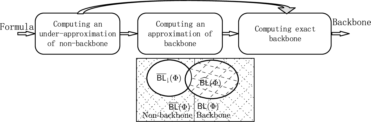
We show the overview of our approach Bone in Fig. 1. Taking a satisfiable formula Φ as an input, Bone first computes a subset of non-backbone ${\overline{BL}}_{⇂} (Φ) \subseteq \overline{BL} (Φ)$ . Then, Bone computes an intermediate set of backbone $\hat{BL} (Φ)$ based on the set ${\overline{BL}}_{⇂} (Φ)$ , where each literal $l \in \hat{BL} (Φ)$ has a high possibility to be a backbone literal of Φ. Finally, Bone removes non-backbone literals from $\hat{BL} (Φ)$ and adds backbone literals into $\hat{BL} (Φ)$ to compute the exact backbone of Φ.

Fig. 1.

Overview of our approach.

As shown in Fig. 1, ${\overline{BL}}_{⇂} (Φ)$ only contains a part of non-backbone literals. Most of the literals in $\hat{BL} (Φ)$ are backbone, only a small part of them is non-backbone. With more known backbone literals, SAT testings are accelerated.

Computing an under-approximation of non-backbone. Given a satisfiable formula Φ, we first compute a model λ of Φ by calling a SAT solver. From the model λ, we compute a base under-approximation of non-backbone. Later, we apply a Greedy-based algorithm to add more non-backbone literals into the base set, which results in ${\overline{BL}}_{⇂} (Φ)$ .

The algorithm iteratively computes new models until no new model can be found. We choose to change the literal that satisfies the least clauses at each iteration, as the number of clauses effected by this literal is the least one, provided a higher possibility to find a new model. K models will be generated after the k iterations. New non-backbone literals are found from each new model. It’s worth noticing that for every literal that has different assignment in all models, we can put them into the under-approximation of non-backbone literals.

Computing an approximation of backbone. At this step, we apply a Whitening-based algorithm to compute an approximation $\hat{BL} (Φ)$ . Whitening Algorithm was used to compute essential nodes that cannot be colored as white without changing the color of its adjacent nodes in a graph coloring problem.

We consider essential nodes as ’possible’ backbone literals in backbone computing. To increase the proportion of backbone literals found by Whitening Algorithm, we use two heuristic strategies to refine Whitening Algorithm. First, we check whether the generated assignment is a model to eliminate some of the non-backbone literals returned by Whitening-based Algorithm. Moreover, we use assumptions features of MINISAT [12] to find some accurate backbone literals. If the conflict size returned by the assumptions features is one, then the negation of the conflict literal is a backbone literal. If the formula is satisfiable under the given assumptions, then we get a new model. By comparing the new model with the old one, we are also able to find non-backbone literals. With the refinement of heuristic strategies, Whitening-based Algorithm is able to return a set of literals that are highly likely to be backbone.

Computing exact backbone. Based on $\hat{BL} (Φ)$ , we test whether a literal $l \in \hat{BL} (Φ)$ is a backbone one by one. A naïve but efficient approach [13] is to test the satisfiability of $Φ \land l$ , and $Φ \land \neg l$ . It’s widely used in backbone computing approaches because of its efficiency, therefore, we implemented an iterative SAT testing approach to compute exact backbone based on the idea of this naïve approach. Iterative SAT testing algorithm uses SAT solvers to test whether a literal is a backbone literal or not. For instance, if $Φ \land \neg l$ is unsatisfiable but Φ is satisfiable, then l must be a backbone literal of Φ.

We use the model $λ ⊧ Φ$ and $\hat{BL} (Φ)$ , ${\overline{BL}}_{⇂} (Φ)$ computed in the previous steps as input. We first iteratively select one literal l from $\hat{BL} (Φ) ∖ {\overline{BL}}_{⇂} (Φ)$ such that $λ ⊧ \neg l$ and test l by checking the satisfiability of $Φ \land l$ (dashed area in Fig. 1). If l is a backbone, we will add l into Φ as a clause. Adding known backbone literals into Φ as clauses potentially speedups the later SAT testing [5,12,19]. If a new model is generated, we are able to find some non-backbone literals by comparing the difference between the newly generated model and the original one. Then, we do the same testing for literals from $L (Φ) ∖ ({\overline{BL}}_{⇂} (Φ) \cup \hat{BL} (Φ))$ (dotted area in Fig. 1). After this step, the exact backbone and non-backbone are found.

Comparing to the approach of directly test all literals in $L (Φ)$ , there are two contributions of Bone. One is that we reduce the number of SAT calls using the known non-backbone literals $\hat{BL} (Φ)$ . The another one is that we first check literals that have high probability to be backbone literals so that backbone literals can be found as early as possible.

4. Greedy-based computing

{\overline{BL}}_{⇂} (Φ)

In this section, we propose an algorithm to compute the under approximation of non-backbone, namely Greedy-based Algorithm. As mentioned in Section 3, Greedy-based Algorithm is a straight forward algorithm which is able, for a given model, to compute parts of non-backbone in quadratic time. It’s able to reduce the number of total SAT calls since literals in ${\overline{BL}}_{⇂} (Φ)$ don’t need SAT testings. Experiments show that Greedy-based Algorithm reduces 5% solving time.

4.1. Computing ${\overline{BL}}_{⇂} (Φ)$ using one model

Computing ${\overline{BL}}_{⇂} (Φ)$ using only one model is equivalent to rotatable literals mentioned in [12]. Given a formula Φ, we first compute a model λ using SAT solver. We then compute the set of non-backbone literals using λ, referred as $L (Φ, λ)$ . To compute $L (Φ, λ)$ , we first find clauses that have at least two satisfied literals and put them into a set, refereed as $Φ_{⊧_{2}}$ . We then scan all literals in $L (Φ)$ , and skip literal l and $\neg l$ if l satisfies a clause $ϕ \notin Φ_{⊧_{2}}$ . The rest literals are in $L (Φ, λ)$ .

Algorithm 1:

Naïve Algorithm: Computing non-backbone literals using λ

Algorithm 2:

Greedy-based algorithm

The only line in this naïve Algorithm is computing the non-backbone literals set of a given model λ.

Theorem 2.

$L (Φ, λ) \subseteq \overline{BL} (Φ)$ .

Proof.

Suppose a literal $l \in L (Φ, λ)$ . According to the Naïve Algorithm, $λ (l) = 1$ , and there must exists a literal $l^{'}$ in any clause $ϕ \in Φ_{l}$ , such that $(l^{'} \in ϕ) \land l (^{'} \neq l) \land (λ (l^{'}) = 1)$ . Therefore, there must exist a model $λ^{'} = λ [\neg l]$ . It concludes that l is a non-backbone literal of Φ, i.e., $l \in \overline{BL} (Φ)$ . Given a formula Φ and a model $λ ⊧ Φ$ , suppose a literal $l \in L (Φ, λ)$ , then for every clause $ϕ \in Φ_{l}$ , there must exists a literal $l_{2}$ such that $l \neq l_{2}$ and $λ (l) = 1, λ (l_{2}) = 1$ . $l_{2}$ is another satisfied literal of ϕ. Therefore, there must exists an assignment $λ [\neg l] ⊧ Φ$ , since all clauses contains l will be continue satisfied by another literal in that clause. □

4.2. Computing

{\overline{BL}}_{⇂} (Φ)

using Greedy-based algorithm

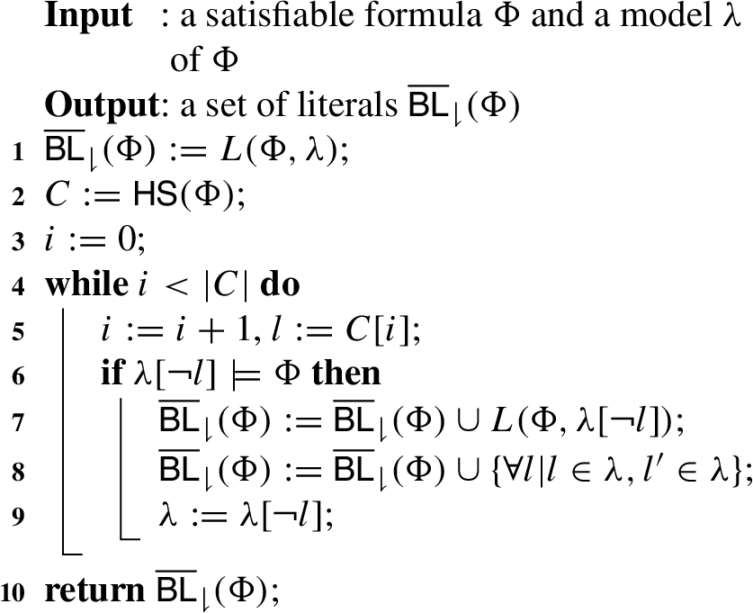
To save more SAT testings, we propose the Greedy-based algorithm shown in Algorithm 2 to get more non-backbone literals. Comparing to Algorithm 1, Greedy-based algorithms is able to compute more non-backbone literals using more models generated from the original model λ. The rotatable literals in [12] is a subset of the result in Greedy-based Algorithm.

We use $HS$ to denote the heuristic strategy of greedy algorithm. In the default Minisat 2.2 setting, the literals are weighted by the number of appearance in clauses initially, revision are made during the solving process according to the number of appearance in conflicts. In Greedy-based Algorithm, we want to find literals that affect the least of the given formula Φ, therefore, the reverse of weighted literals in Minisat 2.2 solver is the correct order of HS that we wished. C is an order set of literals, resulted from the heuristic strategy $HS$ . When changing the assignment of a literal l, the less clauses l satisfies, the less clauses are affected, the higher possibility that a new model is found.

Given a formula Φ and a model λ, we construct the ordered set of literals C according to $HS$ at Line 3. From Line 5, we start to change the assignment of the literal in C one by one. At Line 7, for each selected literal l, we construct a new assignment $λ [\neg l]$ from the model λ and check whether $λ [\neg l]$ satisfies Φ in polynomial time. If $λ [\neg l]$ satisfies Φ, then we add the set of non-backbone literals $L (Φ, λ [\neg l])$ into ${\overline{BL}}_{⇂} (Φ)$ , and assign $λ [\neg l]$ to λ which will be severed as the model of Φ at the next step. With λ changing at every iteration, we are able to obtain more various assignments and find more non-backbone literals. If λ keeps the same at each iteration, we can only obtain the assignments $λ [\neg l], l \in L (Φ)$ , which is not as various as the assignments by changing model λ at every iteration.

Theorem 3.
${\overline{BL}}_{⇂} (Φ) \subseteq \overline{BL} (Φ)$ .
Proof.
Suppose a literal $l \in {\overline{BL}}_{⇂} (Φ)$ , if l is added to ${\overline{BL}}_{⇂} (Φ)$ at Line 2, then $l \in L (Φ, λ)$ , $l \in \overline{BL} (Φ)$ (Theorem 2). Otherwise, l is added to ${\overline{BL}}_{⇂} (Φ)$ at Line 7, we know that there must exists a model $λ^{'}$ , $l \in L (Φ, λ^{'})$ (Line 7). Since $L (Φ, λ^{'}) \subseteq \overline{BL} (Φ)$ (Theorem 2), $l \in \overline{BL} (Φ)$ . It concludes that ${\overline{BL}}_{⇂} (Φ) \subseteq \overline{BL} (Φ)$ . □
Theorem 4.
The complexity of Greedy-based Algorithm from Line 2 to Line 10 is $O (m \times n)$ , where m is the size of $L (Φ)$ and n is the size of clauses in Φ.
Proof.
Given a model $λ ⊧ Φ$ as the input of Greedy-based Algorithm. Started from Line 2, we scan all m clauses to count number of satisfied literals, and scan all n literals to compute $L (Φ, λ)$ . The complexity of Line 2 is $O (m \times n)$ . With the information collected from Line 2, Line 3 will be finished in $O (m^{2})$ time since it needs to sort a set of literals decreasingly according to $HS$ . Line 5 scans all literals, the complexity is $O (m)$ . With the information from Line 2, Line 7 will be finished in $O (1)$ time. The complexity of the loop started from 5 is $O (m)$ . The total complexity of Greedy-based Algorithm is $O (m \times n)$ . □

Greedy-based Algorithm saved 5% solving time in total. With non-backbone literals recognized ahead, SAT testing numbers are reduced. Backbone computing is expediting by the save of SAT testings.
5. Whitening-based computing $\hat{BL} (Φ)$

In this section, we propose an algorithm to compute approximate set of backbone literals $\hat{BL} (Φ)$ , namely Whiten-based Algorithm. As mentioned in Section 3, finding more backbone at the earlier stage of the computing provides benefits for the later backbone computing. Experiments show that the proportions of backbone in $\hat{BL} (Φ)$ are generally higher than that in the original formula. Moreover, 20% solving time is saved by Whiten-based Algorithm.

5.1. Whitening algorithm

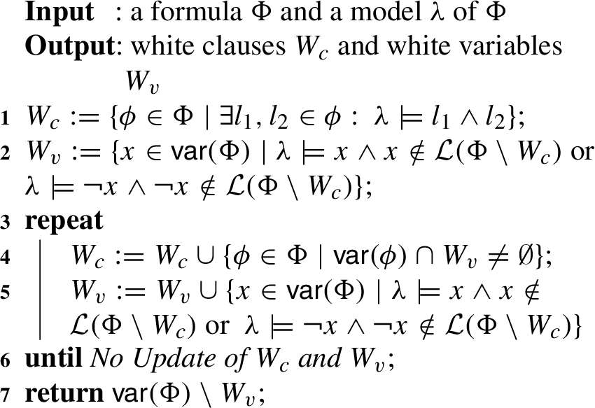
In [9], the authors proposed an Whitening algorithm that computed the essential nodes in a coloring problem named Whitening Algorithm. We propose a Whitening-based Algorithm for ’possible’ backbone (essential) literals computing based on the original one. We use $W_{c}$ to denote the clauses that have at least two satisfied literals to a given model. We use $W_{v}$ to represent a set of variables, every variable x in $W_{v}$ only satisfies clauses in $W_{c}$ . $W_{c}$ and $W_{v}$ are updated concurrently.

We first compute a set of clauses that have at least two satisfied literals under the current model, named $W_{c}$ at Line 2. We find variables that only satisfied clauses in $W_{c}$ , and put them into a set of variables, named $W_{v}$ at Line 3. We then start to iteratively extend $W_{c}$ and $W_{v}$ from Line 4. For every variable $v \in W_{v}$ , if a clause contains $\neg v$ , it will be added to $W_{c}$ at Line 5. After that, we compute $W_{v}$ again with the extended $W_{c}$ . We repeat the procedure until no clause are added to $W_{c}$ . At last, the complement of $W_{v}$ is the set of essential variables. It’s important that no elements are taken away from $W_{c}$ , the algorithm will terminate since the number of clauses is finite.

Given a model λ, the complexity of Whitening Algorithm is polynomial since it doesn’t need SAT testing. For any variable $x \in W_{v}$ , all clauses in $Φ_{\neg x}$ will have at least two satisfied literals in the assignment $λ [\neg x]$ , one is $\neg x$ , the other is one of the satisfied literals of ϕ under λ. In this way, Whitening Algorithm extended $W_{c}$ without SAT testing.

Limited by the only model given to Whitening Algorithm, only a part of backbone variables are in $W_{v}$ . Different models will have different $W_{v}$ . For example, given a formula $\begin{array}{l} (\neg a \lor b \lor \neg c) \land (\neg a \lor \neg b \lor c) \\ \land (\neg a \lor b \lor d) \land (\neg c \lor d) \land (a \lor d) \end{array}$ and a model λ such that $λ (a) = 1 \land λ (b) = 1 \land λ (c) = 1 \land λ (d) = 1$ . At Line 5, $W_{c}$ is initialized with ${(\neg a \lor b \lor d), (a \lor d)}$ . $W_{v}$ is initialized with ${a}$ . The result of Whitening Algorithm is empty set. It indicates that non of the variable is backbone. Actually, d is a backbone literal, since there does not exist a model λ that $λ (\neg d) = 1$ .

Algorithm 3:

Whitening-based algorithm

Given a model λ, the assignment change of a given variable v will generate a new assignment $λ [\neg v]$ . As we record the assignments generated during the compute step by step, we found that a is a non-backbone variable, because $λ [\neg a]$ is another model. $b, c$ are non-backbone variables because $λ [\neg a, \neg b]$ and $λ [\neg a, \neg c]$ are models of the given formula. However, neither $λ [\neg a, \neg b, \neg d]$ nor $λ [\neg a, \neg c, \neg d]$ is a model of the given formula.

We consider that an iteration of a repeat loop ended, if the last line of code in the loop body has been executed. In Algorithm 3, we consider that an iteration of the repeat loop ended when Line 5 was executed. A new iteration of the repeat loop started after that if the terminating condition of the loop hasn’t been satisfied by then.

The detail iteration of Algorithm 3 using the given example are as follows: At Line 1, $(\neg a \lor b \lor d)$ and $(a \lor d)$ were added to $W_{c}$ . $W_{c} = {(\neg a \lor b \lor d), (a \lor d)}$ . At Line 2, only a is added to $W_{v}$ . Variable d was not added to $W_{v}$ since variable d appeared in $(\neg c \lor d)$ , which is not in $W_{c}$ . $W_{v} = {a}$ .

In the first iteration of the repeat loop started from Line 3, we added $(\neg a \lor b \lor \neg c)$ and $(\neg a \lor \neg b \lor c)$ to $W_{c}$ at Line 4. $W_{c} = {(\neg a \lor b \lor d), (a \lor d), (\neg a \lor b \lor \neg c), (\neg a \lor \neg b \lor c)}$ . We added $b, c$ to $W_{v}$ , since all clauses that literal b and literal c appeared were in $W_{c}$ . $W_{v} = {a, b, c}$ . The repeat loop continued at Line 6 since both $W_{c}$ and $W_{v}$ were updated.

In the second iteration, $(\neg c \lor d)$ was added to $W_{c}$ at Line 4, since variable c appears in $(\neg c \lor d)$ . $W_{c} = {(\neg a \lor b \lor d), (a \lor d), (\neg a \lor b \lor \neg c), (\neg a \lor \neg b \lor c), (a \lor d)}$ . At Line 5, we added variable d into $W_{v}$ since all clauses that literal d appeared were in $W_{v}$ . $W_{v} = {a, b, c, d}$ . Since both $W_{v}$ and $W_{c}$ were updated, the repeat loop continued at Line 6.

In the third iteration, no clause was added to $W_{c}$ at Line 4, since all clauses were already in $W_{c}$ . No variable was added to $W_{v}$ at Line 5, since all variables were already in $W_{v}$ . The repeat loop exited at Line 6 because neither $W_{c}$ nor $W_{v}$ updated. The program returned an empty set at Line 7.

5.2. Assignments checking based Whitening algorithm

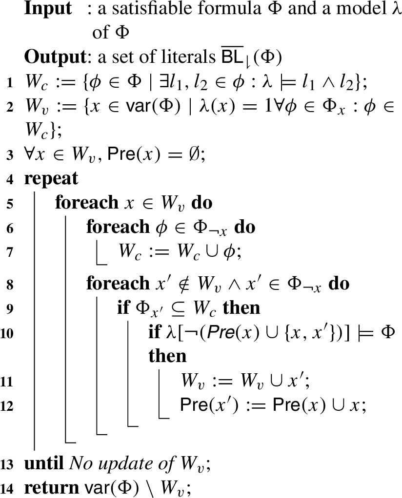
To avoid missing backbone literals like d, we propose a Whitening-check-based Algorithm (WCB for short) to compute the approximation of backbone literals with satisfiability check of each generated assignment. $Pre (x)$ is used to record the literals that changed its assignment at each iteration. With the changed literals, we are able to generate a new assignment at each iteration. We choose a variable $x \in W_{v}$ at each iteration, and update $W_{c}$ by adding $Φ_{\neg x}$ , $W_{v}$ is extended accordingly. For every new variables $x^{'}$ in $W_{v}$ , we test the satisfiability of assignment $λ [\neg (Pre (x) \cup {x, x^{'}})]$ . $x^{'}$ maintains in $W_{v}$ if a new model is found. Otherwise, $x^{'}$ removes from $W_{v}$ . Algorithm stops when there is no new clause added to $W_{c}$ .

Algorithm 4:

WCB Algorithm with Assignment Satisfiability Checking

We compute $W_{c}$ and $W_{v}$ at the first two lines, and extend $W_{c}$ and $W_{v}$ at Line 5. At Line 11, we test whether the generated assignment is a model of the given formula Φ. At each iteration, we change the assignment of $x \in W_{v}$ , it results in adding $x^{'}$ to $W_{v}$ . If the assignment $λ [\neg (Pre (x) \cup {x, x^{'}})]$ passes the satisfiability check at Line 11, $x^{'}$ remains in $W_{v}$ , and $Pre (x^{'})$ is $Pre (x) \cup {x}$ . Otherwise, $x^{'}$ is removed from $W_{v}$ .

The WCB Algorithm finds some missing backbone literals in Whitening Algorithm. Since the test of satisfiability at Line 11 is in polynomial time, the time complexity remains the same.

Theorem 5.

$\forall x \in W_{v}$ , $x \in {\overline{BL}}_{⇂} (Φ)$ .

Proof.

Given a formula Φ and a model $λ ⊧ Φ$ , suppose a variable $x^{'} \in W_{v}$ . If $x^{'}$ is added to $W_{v}$ at Line 3, then there must exists a literal $l = x$ or $\neg l = x$ , for every clause ϕ that contains l, there must exists another literal $l^{'}$ , such that $λ (l^{'}) = 1$ . Therefore, there must exists another model $λ^{'} = λ [\neg l]$ of Φ, x is a non-backbone literal of Φ. If $x^{'}$ is added to $W_{v}$ at Line 12, there must exists a variable x, where a new model $λ [\neg Pre (x) \cup {x, x^{'}}]$ of Φ is generated at Line 11. Therefore, there exists two different models $λ_{1}$ and $λ_{2}$ of Φ, such that $λ_{1} (x^{'}) = 0$ and $λ_{2} (x^{'}) = 1$ . $x^{'}$ is a non-backbone literal of Φ. □

We detail the computation of Algorithm 4 on the same example we used above. The formula in the example is $\begin{array}{l} (\neg a \lor b \lor \neg c) \land (\neg a \lor \neg b \lor c) \\ \land (\neg a \lor b \lor d) \land (\neg c \lor d) \land (a \lor d) \end{array}$

$W_{c}$ was initialized as ${(\neg a \lor b \lor d), (a \lor d)}$ at Line 1, $W_{v}$ was initialized as ${a}$ at Line 2. Pre(a) was initialized as empty set at Line 3. In the first iteration of the repeat loop started from Line 4, x was assigned with a at Line 5, all clauses that contains $\neg a$ were added to $W_{c}$ , $W_{c} = {(\neg a \lor b \lor d), (a \lor d), (\neg a \lor b \lor \neg c), (\neg a \lor \neg b \lor c)}$ .

In the first iteration of foreach loop started from Line 5, and the first iteration of the foreach loop started from Line 8, b was assigned to $x^{'}$ , since all clauses that contains b were in $W_{c}$ , we went to the true branch of Line 9. At Line 10, we tested whether $λ (\neg a, \neg b) = (\neg a \land \neg b \land c \land d)$ is a model of the given formula, b was added to $W_{v}$ at Line 11, since $λ (\neg a, \neg b)$ is a model of the given formula. $Pre (b)$ was assigned with ${a}$ at Line 12.

In the second iteration of the foreach loop started from Line 8, c was assigned to $x^{'}$ , since $(\neg a \lor \neg b \lor c)$ was in $W_{c}$ , which is the only clause containing c, we tested whether $λ (\neg a, \neg c) = (\neg a \land b \land \neg c \land d)$ is a model. $λ (\neg a, \neg c)$ is a model and we added c to $W_{v}$ at Line 11, $Pre (c)$ was assigned with a at Line 12.

At the third iteration of the foreach loop started from Line 8, d was assigned to $x^{'}$ , since $(\neg c \lor d)$ was not in $W_{c}$ , the iteration ended at Line 12, the foreach loop stared from Line 8, and the foreach loop started from Line 5 ended.

In the second iteration of the repeat loop, x was assigned to a and b in the first two iterations of the foreach loop started from Line 6, these iterations ended without changing $W_{c}$ or $W_{v}$ . x was then assigned to c in the third iteration of the foreach loop started from Line 6, $(\neg c \lor d)$ was added to $W_{c}$ after Line 7. In the first iteration of the foreach loop started from Line 8, d was assigned to $x^{'}$ , since $λ (\neg c, \neg d)$ is not a model of the given formula, $W_{v}$ remains the same, at the foreach loop started from Line 8, and Line 5 ended.

In the third iteration of the repeat loop, x was assigned to a, b, and c in each iterations, $W_{c}$ and $W_{v}$ remains the same after all the iterations. There is no update of $W_{c}$ or $W_{v}$ , the repeat loop ended. The program returns ${d}$ at Line 14.

5.3. Computing parts of exact backbone using assumptions

Although WCB Algorithm is able to compute an approximation set of backbone, it still needs at least one SAT testing to determine whether a literal is backbone, which may need a long solving time. Inspired by [12], we use assumptions in MINISAT as a heuristic strategy to accelerate SAT testing, named Whitening-assumptions-based Algorithm, WAB for short.

Experiments show that given the same formula Φ, SAT testings with assumptions are generally faster then the ones without assumptions. It’s because that assumptions help to make the initial decisions of a SAT solving, given an assumption γ with k literals in it, it reduces $2^{k}$ states of the searching spaces. SAT testing with a longer assumptions will return faster.

A formula Φ is satisfiable with assumption γ indicates that there exists a model $λ ⊧ Φ$ , such that $\forall l \in γ$ , $λ (l) = 1$ . We use $SAT (Φ, γ)$ to denote a SAT testing of Φ with the assumption of γ. We use $(b, λ, r)$ to denote the result of $SAT (Φ, γ)$ . If b is assigned to 1, a model is returned in λ, otherwise, a reason of unsatisfiable is returned in r. For every literal $l \in \hat{BL} (Φ)$ , $\neg l$ is selected to γ. If there is exactly one reason $l_{b}$ returned from $SAT (Φ, γ)$ , it indicates that $\neg l_{b}$ must be a backbone of Φ.

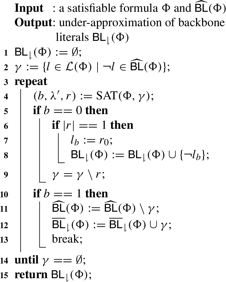
Given a model λ and a satisfiable formula Φ. We initialize γ with $\hat{BL} (Φ)$ at Line 3. We add $\neg l$ to γ for every $l \in \hat{BL} (Φ)$ to block the known model λ. At Line 5, we compute the result of $SAT (Φ, γ)$ . All literals in γ will be removed from $\hat{BL} (Φ)$ at Line 12 if b is assigned to 1. Otherwise, all literals in r are removed from γ at Line 10. Once γ is empty, the iteration stops. If there is exactly one literal $l_{b}$ in r, $\neg l_{b}$ must be backbone and added to ${BL}_{⇂} (Φ)$ at Line 9.

Theorem 6.
Given a satisfiable formula Φ and a set of assumptions γ, $\neg l_{b} \in BL (Φ)$ if $l_{b} \in γ$ and $l_{b}$ is the only reason that Φ is not satisfiable under the assumption of γ.
Proof.
Given a satisfiable formula Φ and a set of assumptions γ, suppose literal $l_{b}$ is the only reason returned r from $SAT (Φ, γ)$ , i.e., $\forall l \in r, l = l_{b}$ . It means that there doesn’t exist a model $λ ⊧ Φ$ , such that $λ (l_{b}) = 1$ . Therefore, $\neg l_{b}$ is a backbone literal of Φ, i.e., $\neg l \in BL (Φ)$ . □

WAB Algorithm (Algorithm 5) is able to compute the approximation of backbones of the given formula. When the length of unsatisfiable reason is 1, WAB saved solving time when determining if a variable is a backbone. Experiments show that, SAT testings with assumptions are generally finished within 1 second, while original SAT testing may take more than 1 minute.

Compared with the original Whitening Algorithm, the accuracy of Whitening-based Algorithm improved by two heuristic strategies (WCB and WAB) has increased. Missing backbone are added to the approximation through WCB and accurate backbone are confirmed with WAB. With a higher accuracy, backbone computing are guided better with $\hat{BL} (Φ)$ .

Algorithm 5:
WAB Algorithm for computing under-approximation of backbone ${BL}_{⇂} (Φ)$

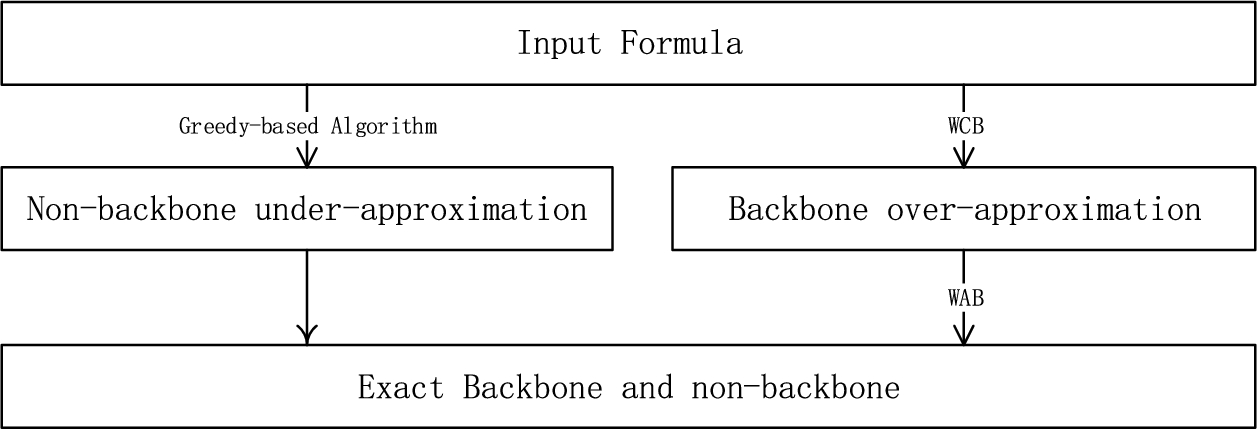
In Bone, we first compute the under-approximation of non-backbone literals ${\overline{BL}}_{⇂} (Φ)$ , using Greedy-based Algorithm. Then we compute an over-approximation $\hat{BL} (Φ)$ of backbone literals using WCB, we use WAB to find exact backbone and non-backbone literals in the $\hat{BL} (Φ)$ . The scheme graph is shown in Fig. 2.

Fig. 2.
Scheme Graph of Bone.
6. Experimental study

To study the performance of Bone, we compare it to state-of-the-art tool Minibones [12] and analysis total solving time for different groups of formulae. Different algorithms are implemented in Minibones. We choose the best algorithms of Minibones recommended by the author in [12], namely, $CoreBased$ algorithm with a chunk size of 100.

We implemented Bone in C++ interfacing MINISAT 2.2 [6].The experiments were conducted on a cluster of IBM iDataPlex 2.83 GHz, each industrial formula was running with a memory limit of 4 GB. Each random formula was running with a memory limit of 256 MB.

In the experiments, we separate formulae into groups based on different applications. We study the performance of Bone in 3 different groups, under different time limits. In 3600 seconds, results show that Bone saved 21% solving time in total and performs the best in $manthey$ group, saving 34% of solving time. In 16000 seconds, results show that Bone solved 2 more formulae (49 formulae) than Minibones does.

Experiments show that both Bone and Minibones are good at solving industrial formulae which have clear partitions of variables. In the experiments of random formulae, results indicate that Bone is good at solving formula with more variables that have over 10 adjacent variables.

6.1. Benchmark setup

We select 784 crafted and industrial formulas from SAT competitions between 2002 and 2016. 291 formulas can’t find a model using Minisat 2.2 in 3600 seconds. 196 formulas are unsatisfiable formulas, which do not have any backbone.

To study the performance difference between Minibones and Bone under different formula group, we choose three industrial groups: $mrpp$ , $manthey$ and $dimacs$ . $mrpp$ comes from multi robot path planning problems, $manthey$ comes from finding gray codes problems, these codes might attack encryptions, and $dimacs$ comes from graph problems. These groups are neither nor too hard. Both Bone and Minibones need more than 5 seconds to solve the formulas in these groups. In every group, $2 / 3$ formulas can be solved by Minisat 2.2 in 3600 seconds. Both Bone and Minibones use Minisat 2.2 as SAT solving, solving by Minisat 2.2 is the basis of finishing finding backbone literals.

Fig. 3.

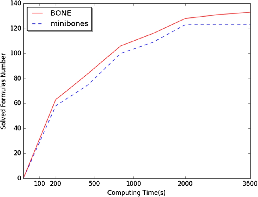
Numbers of Solving Formulas of Minibones and Bone.

6.2. Means of presentation

We use $st$ to denote the solving time and $sc$ to represent SAT testings number. Comparisons of solving time among individual formula are shown as plots figures. In the figures, each line represents a tool performance of the formulae. The x-axis stands for the individual formula and the y-axis stands for the solving time of the corresponding formula.

6.3. Experimental results on industrial formulae

Bone solved 132 formulas in 3600 seconds, while Minibones solved 123 formulas. All formulas solved by Minibones are also solved by Bone. Bone solved 9 more formulas than Minibones. Figure 3 shows the number of solved formulas of Minibones and Bone. The x-axis is solving time (seconds), the y-axis is the number of formulas that Minibones and Bone can solved under this time limitation. The red line stands for the solving formulas number of Bone and the blue dotted line stands for the solving formulas number of Minibones. As we can observe, Minibones solved less formulas than Bone under a longer time limitation, it indicates that Bone has a better scalability than Minibones when the formulas requires a longer time to solve.

Consider the formulas that are solved by both Minibones and Bone, the total SAT testing number and solving time are listed in Table 1. Bone saved 7% solving time than Minibones. Bone saved 43% SAT testing numbers than Minibones. It indicates that Bone saved solving time by saving SAT testing.

Table 1
Total Solving Time and SAT Testing Number of Minibones and Bone

Tool $st$ (s) $sc$

Bone 35779 1860897

Minibones 38497 3246679

Tool	$st$ (s)	$sc$
Bone	35779	1860897
Minibones	38497	3246679

To study the performance difference in different problems, we analyze the result of formulas in $mrpp$ , $manthey$ , $dimacs$ groups. Among the 72 industrial formulae, both Bone and Minibones are able to solve 34 of them in 3600 seconds (1 hour). If more solving time is provided, Bone solved 49 formulae in 16000 seconds (almost 5 hours) while Minibones solved 47 formulae. The details of solving time and SAT tests number comparison of each group are shown in Table 2, and Table 3 (with 1 hour time limits). The st of Difference is the one minus division between st of Bone and st of Minibones, indicating how much solving time has been saved by Bone.

Table 2

Solving Time Comparison on Industrial Formulae

Benchmark	$st$ of Bone(s)	$st$ of Minibones (s)	$st$ Difference
mrpp	6112	6900	11%
manthey	4845	7363	34%
dimacs	1339	1369	2%
total	12296	15632	21%

Table 3

Number of SAT Testings Comparison on Industrial Formulae

Benchmark	$sc$ of Bone(s)	$sc$ of Minibones (s)	$sc$ Difference
mrpp	28261	28839	3%
manthey	49356	72943	33%
dimacs	2018	2042	1%
total	79635	103224	23%

Solving time and SAT testings number of these three groups are listed in Table 2, and Table 3. We can observe that Bone performs the best on $manthey$ group, saved 34% solving time, with 33% saving on SAT testings. In total, Bone saved 21% solving time and 23% SAT testings. Bone saved 11% solving time and 3% SAT testings in $mrpp$ group, while saving 2% time and 1% SAT testings in $dimacs$ group. It proves the observation in [12] from experiment concepts that less SAT testing will lead to a faster solving.

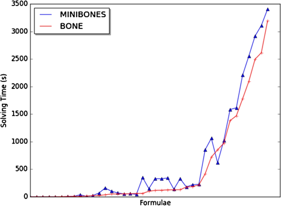
Figure 4 shows the solving time of all 34 industrial formulae. The x-axis represented the id of the formula, the y-axis represented the solving time (seconds). The blue line shows the solving time of Minibones, each small triangle represents the solving time of the corresponding formula. While the red line represented the solving time of Bone, each cross represents the solving time of the corresponding formula using Bone. As we can observe, there are only 3 formulae that Minibones outperforms Bone.

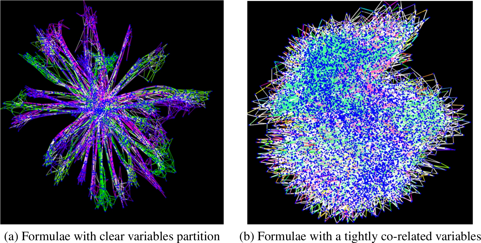
When we take a look at the formulae in $manthey$ group that Bone performs the best, we find that they all have a star-like adjacent structure as shown in Fig. 5(a). It means that the variables is separate into different partitions, different variables from different partitions only appears in a few clauses at the same time. Each branch in the graph stands for a partition.

Fig. 4.

Solving Time Comparison on Industrial Formulae.

Figure 5(b) is the adjacent structure of formulae that can’t be solved in 16000 seconds using both tools. It’s obvious that there is no clear partition among the variables.

Fig. 5.

Figure (a) shows the star-like adjacent structure, indicates that variables separate into individual partitions, both Bone and Minibones are able to solve these formulae in 3600 seconds, Bone saved 34% solving time in total. Figure (b) shows the adjacent structure with a core and no branches, indicates that variables are tightly co-related in the formula. These formulae are more complex than the formula in 5(a), Bone solved 2 more formulae than Minibones among these formulae, within 16000 seconds.

For industrial formulae, Bone performs better than Minibones in general. We also found that the performance of Bone and Minibones are related to the adjacent structure of the given formula. A formula with clear partitions of variables tend to performs better on both Bone and Minibones.

6.4. Result analysis

Iterative SAT testings, which will hold the assignment of a literal l using assumptions, take the major part of solving time in Bone. Different solving trees will be generated when choosing different l. The SAT testing will be faster if a SAT solving tree is able to find conflicts earlier. Conflicts will be found earlier if the chosen literal l is a backbone literal and mainly appears in a small part of the clauses in the formula, due to the reducing of searching clauses. Therefore, given a formula Φ in $manthey$ group, iterative SAT testing of a backbone literal $l \in BL (Φ)$ will be faster since Φ has a clear partitions of variables and each backbone literal mainly appears in a subset of $cls (Φ)$ . In this way, computing $\hat{BL} (Φ)$ in Bone performs better on formulae in $manthey$ group. There is no big difference of ${\overline{BL}}_{⇂} (Φ)$ performance among groups since the computing time that ${\overline{BL}}_{⇂} (Φ)$ is only related to the numbers of clauses and variables of the formula.

Intuitively, given a formula Φ a model $λ ⊧ Φ$ , a literal l, $λ (l) = 1$ , l can be determined using a unique SAT testing $\neg l \land Φ$ . In our Greedy-based, WAB Algorithm, and Minibones Algorithm, a non-backbone (backbone) literal l could be determined without using $\neg l \land Φ$ . We calculate the number of literals that determined as non-backbone (backbone) literals without using unique SAT testing in Bone and Minibones. The number comparison of these literals in Bone and Minibones are listed in Table 4. We use $pl$ to present these literals. We say that a literal is pruned by Bone or Minibones, if no unique SAT testing are needed in determining the literal. The difference row presents how much more literals that Bone has pruned than Minibones.

Table 4
Number of Literals Determined without Unique SAT Testing in Minibones and Bone

Benchmark Average Literals Number $pl$ of Minibones $pl$ of Bone $pl$ Difference

mrpp 6163 858 782 9%

manthey 2457 1739 1638 6%

dimacs 5087 638 276 57%

total 13707 3235 2696 17%

Benchmark	Average Literals Number	$pl$ of Minibones	$pl$ of Bone	$pl$ Difference
mrpp	6163	858	782	9%
manthey	2457	1739	1638	6%
dimacs	5087	638	276	57%
total	13707	3235	2696	17%

7. Related work

There are basically two types of backbone computing algorithms, model enumeration and literals testing. Model enumeration tries to find every model of the given formula, it uses SAT solvers as oracles. Zhu et al. proposed an iterative SAT testing based algorithm [26,27] and applied to fault localisation, experimental results demonstrate that the use of backbone reduced the size of searching space of it, such as sliding windows and trace buffer. In this algorithm, an upper bound of backbone estimation is refined by enumerating the models of the given formula. Bone computes the non-backbone subset at the first step, which is the complement of upper bound of backbone estimation.

Literals testing decide whether a set of literals are backbone based on the procedure of SAT solving. Kaiser and Kühlin proposed algorithms for computing backbones [13] using SAT solvers. It tries to reduce SAT testings by reusing the previous SAT testing results. Since it is based on SAT techniques, it is still applicable when BDDs reach their space limits. It have been applied to automotive product data verification. Bone is able to generate more models without SAT testing than this algorithm. Climer et al. proposed a graph-based approach to discover backbones which approximates lower and upper bounds to compute backbones [3]. It is able to consistently find two to three more times backbone than previous work CDT [2]. It’s an algorithm using geometry techniques, which is similar to analysing the procedure of SAT solving.

Marques-Silva et al. investigated algorithms for computing backbones emphasizing the integration of existing algorithms which include model enumeration, iterative SAT-testing and filtering with modern SAT solvers, as well as optimisations. They conducted an experimental evaluation of existing techniques and showed that backbone computation for large practical formulae is feasible, with over 70,000 variables and 250,000 more clauses. [11,12,15]. The $CoreBased$ Algorithm with a chunk size of 100 is selected and recommend by the author, which is also the configuration of Minibones in our experiments.

Bone is a combination of model enumeration and literals testing. Greedy-based Algorithm enumerates a set of models based on a given model λ, the literals that are not always assigned to 1 are added to ${\overline{BL}}_{⇂} (Φ)$ . Whitening-based Algorithm computes a set of ’possible’ literals $\hat{BL} (Φ)$ by analyzing the solving procedure with assumptions, which consists of literals. Through analyzing the unsatisfiable reason of a SAT testing, we are able to find a part of accurate backbone and a set of literals that are more possible to be backbone. Experiments demonstrate that the proportions of backbone in $\hat{BL} (Φ)$ are generally higher than that in the original formula. Moreover, comparing to Minibones, with the best configuration selected by the author of it, 15% solving time are saved by testing the literals in $\hat{BL} (Φ)$ first.

For applications, Dubois and Dequen proposed a heuristic search based on backbone information of hard 3-SAT formulae. It’s able to solve unsatisfiable formula with more than 700 variables, which yields DPL-type algorithms with a significant performance improvement over the best previous algorithms [5].

Another work similar to Greedy-based Algorithm in Bone is model rotation, introduced in [1,16]. Model rotation is used to compute MUS of an unsatisfiable formula. New transition clause were found by rotating the literals in the previous transition clause. All MUS must contain transition clause, experiments show that model rotation techniques found more than a half transition clauses in MUS computing, saved 75% computing time without increasing the length of MUS.

8. Conclusion and future work

In this paper, we proposed a backbone computing approach named Bone, using Greedy-Whitening based algorithm. First, we computed an under-approximation of non-backbone ${\overline{BL}}_{⇂} (Φ)$ using Greedy-based Algorithm which is able, for a given model, to compute a part of non-backbone in quadratic time. Literals in ${\overline{BL}}_{⇂} (Φ)$ didn’t need an iterative SAT testing which can save of solving time. Next, we computed an approximation of backbone $\hat{BL} (Φ)$ using Whitening-based Algorithm. The elements in $\hat{BL} (Φ)$ would be backbone with high possibility. We iteratively extended the set of clauses $W_{c}$ and variables $W_{v}$ accordingly. $\hat{BL} (Φ)$ was the complement of $W_{v}$ . Experiments showed that the proportions of backbone in $\hat{BL} (Φ)$ were higher than that in the original formula. Finding more backbone earlier will expedite backbone computing. It’s because that more known backbone can prune more states in SAT solving. At last, we iteratively confirmed backbone from previous approximations.

We compared Bone with state-of-art tool Minibones, on both industrial formulas and crafted formulas. Experimental results for industrial formulae demonstrated that both Bone and Minibones were able to solve 34 formulae from 72 formulae in 3600 seconds. Among the three industrial groups, Bone saved 21% solving time in total than Minibones does. Bone performed the best in $manthey$ group. For every formula in $manthey$ , Bone needed less solving time than Minibones does. Bone solved 49 formulae while Minibones solved 47 formula when the time limit was 16000 seconds. In general, Bone performs better on formulae with clear variables partitions.

There were two major strategies used in Greedy-Whitening Algorithm, experiments showed that they performed differently on different benchmarks when applied independently, it opens a possibility for portfolio approach. How to decide which strategy to use on a given benchmark is the most important part portfolio approach.

In the future, we will try to apply the whitening algorithm to other existing backbone computing approaches. Whitening algorithm is an approximation algorithm which can find a more exact upper bound of backbone literals, it can be applied as the pre-processing method for other backbone computing algorithms. Another future work is to explore the use of satisfying partial assignment in backbone computing. A satisfying partial assignment, no clause in the formula will be assigned to false under the satisfying partial assignment. Backbone computing efficiency may be improved since the computing of satisfying partial assignment is in polynomial time, while the compute of a model is a NP-hard problem.

Footnotes

Acknowledgements

This work is supported the by the program of Theoretical and Practical Research about Linear Time Logic (LTL) Satisfiability (61572197) from National Natural Science Foundation of China (NSFC).

References

Belov and

Marques-Silva, Accelerating MUS extraction with recursive model rotation, in: Formal Methods in Computer-Aided Design (FMCAD), 2011.

Carpaneto,

Dell’Amico and

Toth, Exact solution of large-scale, asymmetric traveling salesman problems, ACM Transactions on Mathematical Software (TOMS) (1995).

Climer and

Zhang, Searching for backbones and fat: A limit-crossing approach with applications, in: Proceedings of the Eighteenth National Conference on Artificial Intelligence (AAAI-02) /Proceedings of the Fourteenth Innovative Applications of Artificial Intelligence Conference on Artificial Intelligence (IAAI-02), 2002.

Culberson and

I.P.

Gent, Frozen development in graph coloring, Theoretical Computer Science (2001).

Dubois and

Dequen, A backbone-search heuristic for efficient solving of hard 3-SAT formulae, in: Proceedings of the Seventeenth International Joint Conference on Artificial Intelligence (IJCAI-01), 2001.

Eén and

Sförensson, An extensible SAT-solver, in: International Conference on Theory and Applications of Satisfiability Testing, 2003.

M.R.

Garey and

D.S.

Johnson, A Guide to the Theory of NP-Completeness, WH Freemann, New York, 1979.

I.P.

Gent and

Walsh, The SAT phase transition, in: Proceedings of European Association for Artificial Intelligence (ECAI), 1994.

Giorgio, On local equilibrium equations for clustering states, Technique Report cs.cc/0212047, 2003.

10.

Janota, SAT solving in interactive configuration, 2010.

11.

Janota,

Lynce and

Marques-Silva, Experimental analysis of backbone computation algorithms, in: International Workshop on Experimental Evaluation of Algorithms for Solving Problems with Combinatorial Explosion (RCRA), 2012.

12.

Janota,

Lynce and

Marques-Silva, Algorithms for computing backbones of propositional formulae, AI Communications (2015).

13.

Kaiser and

Kühlin, Detecting inadmissible and necessary variables in large propositional formulae, University of Siena, 2001.

14.

Kilby,

Slaney and

Walsh, The backbone of the travelling salesperson, in: Proceedings of the Nineteenth International Joint Conference on Artificial Intelligence (IJCAI-05), 2005.

15.

Marques-Silva,

Janota and

Lynce, On computing backbones of propositional theories, in: Proceedings of European Association for Artificial Intelligence (ECAI), 2010.

16.

Marques-Silva and

Lynce, On improving MUS extraction algorithms, in: International Conference on Theory and Applications of Satisfiability Testing, 2011.

17.

M.E.B.

Menaı, A two-phase backbone-based search heuristic for partial MAX-SAT – An initial investigation, in: International Conference on Industrial, Engineering and Other Applications of Applied Intelligent Systems, 2005.

18.

M.E.B.

Menaı, A backbone-based co-evolutionary heuristic for partial MAX-SAT, in: International Conference on Artificial Evolution (Evolution Artificielle), 2005.

19.

Mencıa,

Previti and

Marques-Silva, Literal-based MCS extraction, in: Proceedings of the Twenty-Fourth International Joint Conference on Artificial Intelligence (IJCAI-15), 2015.

20.

Monasson,

Zecchina,

Kirkpatrick,

Selman and

Troyansky, Determining computational complexity from characteristic phase transitions, Nature (1999).

21.

Montanari,

Ricci-Tersenghi and

Semerjian, Solving constraint satisfaction problems through belief propagation-guided decimation, arXiv preprint, 2007, arXiv:0709.1667.

22.

Selman,

Kautz and

Cohen, Local search strategies for satisfiability testing, in: Cliques, Coloring, and Satisfiability: Second DIMACS Implementation Challenge, 1993.

23.

Walsh and

Slaney, Backbones in optimization and approximation, in: Proceedings of the Seventeenth International Joint Conference on Artificial Intelligence (IJCAI-01), 2001.

24.

Zhang and

Looks, A novel local search algorithm for the traveling salesman problem that exploits backbones, in: Proceedings of the Nineteenth International Joint Conference on Artificial Intelligence (IJCAI-05), 2005.

25.

Zhang,

Rangan and

Looks, Backbone guided local search for maximum satisfiability, in: Proceedings of the Nineteenth International Joint Conference on Artificial Intelligence (IJCAI-03), 2003.

26.

C.S.

Zhu,

Weissenbacher and

Malik, Post-silicon fault localisation using maximum satisfiability and backbones, in: International Conference on Formal Methods in Computer-Aided Design, 2011.

27.