INNAMP: An incremental neural network architecture with monitor perceptron

Abstract

This paper proposes a new architecture for supervised incremental learning using neural networks. The key feature of this architecture is a special perceptron, called monitor perceptron, which decides whether a new sample belongs to a new class or to one of the known (already learnt) classes. In case if the decision by the monitor perceptron is that the sample belongs to a new class then the network is extended such that the new class is learnt by the network. The final network is a set of parallel neural networks (one for each class) whose output is fed into the monitor perceptron. A series of experiments are performed using benchmark data sets. The results obtained in these experiments are comparable with or better than those obtained using other, state of art, techniques. The growth in number of neurons is linear with respect to the growth of number of classes.

Keywords

Incremental learning neural network perceptron

1. Introduction

Conventional supervised machine learning approaches work on data where the number of classes are known a priori. However, this condition may not be true in many real world scenarios where new samples may arrive and the machine may not know whether these samples belong to one of the known (already learnt) classes or whether the new sample belongs to a class that has not been learnt yet. In these situations we need an approach which can perform the following:

realize that the newly arrived sample belongs to a new, previously unseen class and

adapt the model so as to learn the new class.

Lazy classifiers like the Nearest Neighbor Classifier (NNC) [16,19] can easily perform the second task but it cannot perform the first task. Most of the other conventional classifiers would classify the new sample into one of the known classes on the basis of the models that it has learnt at the time of training. Thus, they can perform neither of the above tasks.

In case the newly arrived sample has a class label that is new, then the conventional classifiers will re-learn the models. Quite often, this re-learning starts from the beginning i.e. it has to forget the already learnt model in order to learn the new model. This is known as catastrophic forgetting [3,21]. Ideally, we would like to have systems that can perform the two tasks as given earlier and the adaptation of the system should be with minimal changes to the existing system. The dilemma here, known as the stability-plasticity dilemma, is that we want the system to be plastic such that it can learn the new class but also remain stable with respect to the already learnt classes [21].

Several techniques have been proposed earlier which can adapt to changes [3,10,12,20] and are able to solve the problem of stability-plasticity dilemma to a certain extent. However, most of these approaches are unable to decide whether a newly arrived sample belongs to a new class or whether it belongs to one of the known classes.

This statement can be understood if we consider a simple example. Let us consider a Multi-Layer Perceptron (MLP) that needs to be trained to classify samples from five classes (say C1, C2, …, C5). Now, if we assume that instead of training the MLP with training samples from all the five classes, we train the system with samples from only four of the classes, say C1, C2, C3 and C5. If we now present this MLP with samples from C3 then the trained system does not have any mechanism by which it can determine that the samples belong to a class that it has not encountered yet. It will simply declare the samples as belonging to any one of the classes that it has been trained for. Further, even if we want to retrain the system for the samples from the new class (C3 in the present example) then we shall have to retrain the entire system. This happens because the classes C1, C2, C4 and C5 will occupy the entire feature space and there is no room left to accommodate the samples from C3. We shall elaborate on this example in more detail in the third section where we will describe our architecture.

In this paper we present an architecture for supervised incremental learning, using neural networks, which can differentiate between samples that belong to known and previously unseen class. In case the sample belongs to a known class then the system simply classifies the data. On the other hand, if the sample belongs to a previously unseen class, then the network is expanded and adapted so that the new class is learnt by the system. Moreover, the extensions to the network are performed in a controlled manner so that the stability-plasticity dilemma is resolved satisfactorily [21]. As will be shown in the fourth section, the nature of adaptation is such that only small changes are required for some of the classes and most of the classes remain unaffected due to the arrival of samples of the new class. Thus, the major advantages of the proposed architecture are:

The system is able to recognize the fact that a newly arrived test sample is from a class that the system has not learnt yet.

The system is able to expand and adapt so that it can learn to recognize the samples from the new class i.e. add the new class to its knowledge base without changing its existing knowledge base significantly.

The expansion of the system is very controlled and is, in fact, linear with respect to the number of classes.

There are no free parameters that need to be adjusted for different data sets.

The proposed architecture consists of four layers. The first layer is the input layer that simply fans the input to all the neurons of the second layer. The second layer has a set of MLPs [39,42] operating in parallel. The number of MLPs is equal to the number of known (already learnt) classes i.e. each MLP is dedicated to one particular class. Each MLP has one output neuron. The purpose of each MLP is to decide whether a newly arrived sample belongs to the class to which that MLP is dedicated.

The novel aspect of the proposed architecture is the third layer that consists of a single perceptron, called the monitor perceptron. The monitor perceptron accepts the outputs of the MLPs in the second layer and decides whether the newly arrived sample belongs to one of the existing classes or to a new class. Basically, the monitor perceptron has the responsibility of saying “I don’t know” when a new sample belongs to a previously unseen class. In case the sample belongs to one of the known classes, then the outputs of the second layer and the monitor perceptron are sent to the fourth layer which performs the classification and outputs the class label. In case the monitor perceptron says “I don’t know” then the system is expanded by adding one more MLP in the second layer because “for incremental learning, model complexity must be variable” [19].

A series of experiments have been performed on different benchmark data sets taken from the UCI machine learning repository [25]. The results obtained in these experiments are very promising and, in most of the cases, they are more accurate than the existing, state of art, methods while in other cases our results are comparable to those obtained with other methods. We also compare our results with existing incremental techniques and simple multilayer perceptron network and observe similar findings.

This article is organized in the following format. A brief review of existing techniques for incremental learning using neural networks has been presented on Section 2. Section 3 contains details of the proposed architecture along with the motivation behind the architecture. Results of the experiments are presented in Section 4. Finally, conclusions are presented in Section 5.

2. Related work

There have been several approaches to incremental neural networks [7,10,11,20,28,34,36] in the past to satisfy the stability-plasticity dilemma. Different authors have used different methods for achieving the same.

Grossberg presented an unsupervised method called Adaptive Resonance Theory (ART) [21] which was extended for supervised learning and renamed as ARTMAP [10]. There are two ART structures at the base of ARTMAP. Extensive experiments by various researchers have shown that this architecture is sensitive to statistical overlapping between the classes. This sensitivity could also lead to uninhibited growth, which is sometimes referred to as category proliferation. This proliferation results in high computational complexity as well as high memory consumption. It also degrades the classification performance. Several modifications to the original ARTMAP have been proposed like Ellipsoid ART [4] and fuzzy ARTMAP [2,9] which reduces the above problem to some extent. A second issue observed with ARTMAP is deciding the value of the vigilance parameter which governs the decision as to when we should add a new cluster. Model prediction process is like a black box in ART based systems [40].

Some techniques have been proposed which use addition of new neurons for learning new data [5,20,22]. However, it has been observed that adding new neurons to acquire new knowledge leads to huge networks which lead to huge amount of memory requirements and computational cost. Some authors prune unused neurons (neurons that are not making substantial change to network response) from the network along with adding new neurons to the network if necessary so that network size may stay under control [15] and the size of the network remains optimal.

Another method uses incremental singular value decomposition to learn new data [1] for fixed number of output classes. Evolution based schemes for learning in neural nets have also been examined [32]. These techniques use mutation, crossover on fittest network to produce off springs. Huang and Chen presented an incremental neural network based on extreme learning machine [23]. Wang and Wang proposed an interesting technique where they used a combination of small networks for classification [37]. J.L. Calvo-Rolle et al. presented an online learning algorithm for automatic control system using two layer feedforward networks [8].

Probabilistic Neural Network (PNN) [35] has also been used for incremental probabilistic neural network [6,12]. However, the size of the network increases with time. Therefore, it needs huge amount of space for storage and high computational cost. A modified version of PNN was also introduced [11] that has a reduced architecture and provides some savings in terms of memory requirements.

Apart from uncontrolled growth of the network, a problem plaguing most of the existing systems is that they are sensitive to the order in which training data are processed by the network [10]. Adding new data to the network decreases the learning capacity of the network in some cases.

There are some Learning Vector Quantization (LVQ) [24] and k-Nearest Neighbor classifier (KNN) [16] based approaches which can learn within class incremental learning along with between class learning during training [14,33,38].

Incremental Class Learning (ICL) is a technique where we break the problem into sub-problems and train our network for one sub-problem at a time. We then freeze the weights of structure/structures which play a critical role in recognition and add another class [26]. Another sub-problem (new data) based approach has also been proposed by Murphey et al. [27]. In this approach the new data is first passed through the existing network. If the error is below a threshold then no changes are done to the network. However, in case the error is above the threshold then we need to train a new committee of networks and add them to the existing system. The error is then recalculated. If performance improves then we accept the new network otherwise reject them.

Fuzzy neural networks are also used for incremental learning [13,29,41]. These networks are used in a wide variety like with ARTMAP [2,13], MLP [31] or some other neural combinations [29,41].

Our method can be viewed as a member of constructive algorithms [17,18]. It is somewhat similar to the Cascade-Correlation algorithm where the machine learns by adding new hidden neurons to the network one by one. In the Cascade-Correlation method, when we add a new hidden neuron then we freeze all other weights of previously added neurons so that it cannot affect previously learnt data [17].

The discussions in this section show that there is a requirement of experimenting with new architectures in order to overcome the short comings of the existing techniques. We shall now proceed to describe our architecture in the next section.

3. Incremental artificial neural network with monitor perceptron

In previous section we see various approaches of incremental neural network and observe that there is scope for some improvement. In this section we first describe the motivation behind the INNAMP architecture followed by the INNAMP architecture.

3.1. Motivation for INNAMP

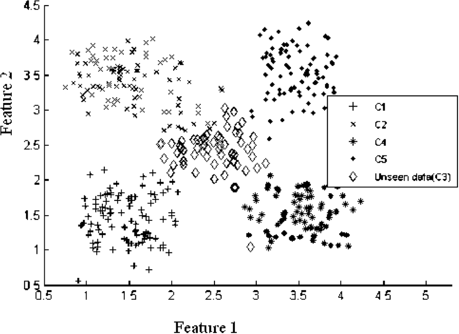
Let us consider the following example in order to understand why conventional neural network architectures like Multi-Layer Perceptrons (MLP) cannot handle the new classes, once it has been trained for a set of classes. In this example we have five classes (C1–C5) as shown in Fig. 1 above with two features ‘Feature 1’ and ‘Feature 2’. We generate this data using Gaussian distribution as given in Eqn. 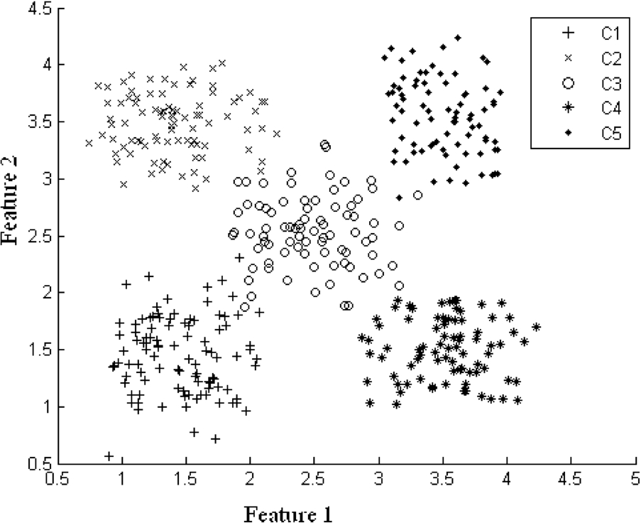(1) where $(x_{i 0}, y_{i 0})$ represents the center of the ith class and $(σ_{i x}, σ_{i y})$ represents the standard deviation of the samples of the ith class around its center. $\begin{matrix} (1) & g_{i} (x_{i}, y_{i}) = e^{(\frac{{- (x_{i} - x_{i 0})}^{2}}{2 σ_{i x}^{2}} - \frac{{(y_{i} - y_{i 0})}^{2}}{2 σ_{i y}^{2}})} \end{matrix}$

Fig. 1.

Initial class distribution.

When we train a standard MLP for the above data we get decision boundaries as shown in Fig. 2. It is clear from the figure that if any class is surrounded by other classes then we get a bounded region for that class as can be seen for class C3; otherwise the decision regions are unbounded as is the case with C1, C2, C4 and C5.

Fig. 2.

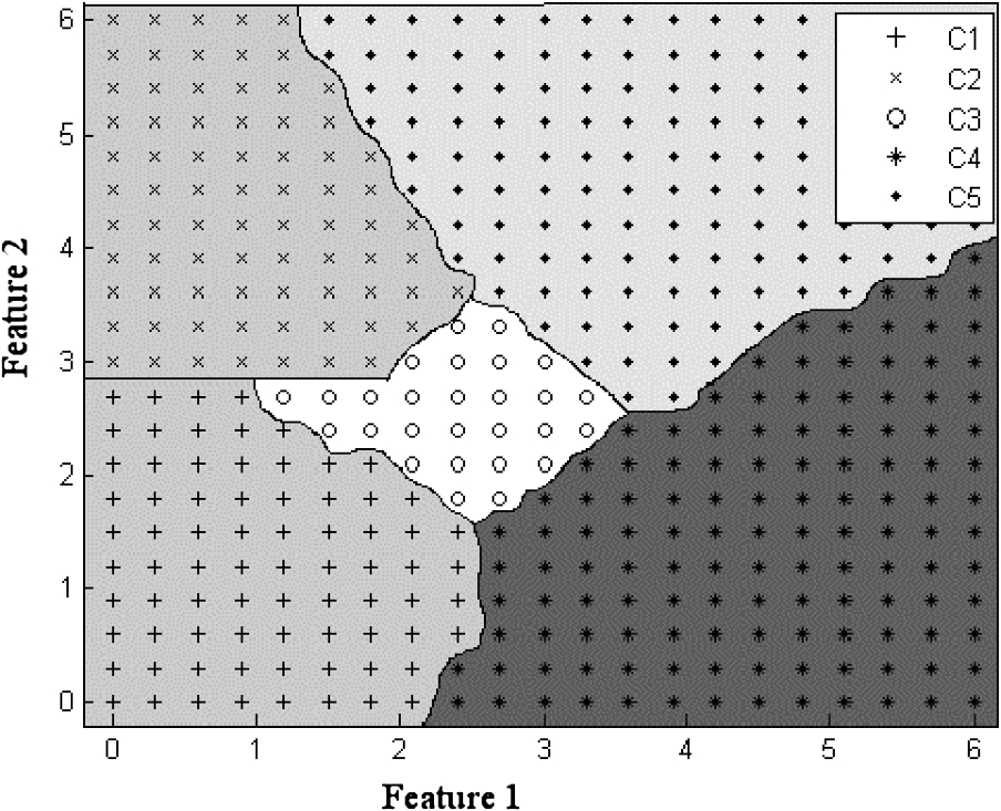
Class boundary using standard MLP.

These bounded and unbounded regions classify all other data (unseen data or new class data) into one of the existing classes. There is no mechanism by which such systems can identify whether a new data belongs to one of the existing classes or whether it belongs to a new class. Moreover, even if we have the information that the newly arrived samples belong to a new class, then we have to retrain the entire system because the decision regions will change quite drastically.

The above statement can be understood by performing an experiment that consists of training an MLP with samples from only four of the five classes namely C1, C2, C4 and C5. The resultant class boundaries are shown in Fig. 3. 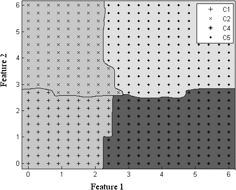Now it is clear from the figure that if we present samples of C3 to this MLP then it classifies these samples into one of the existing classes and classification error rate is $100 %$ for all these samples. A similar result would be obtained even if the samples of C3 lay in a different region of the feature space since the decision regions of the already learnt classes (i.e. C1, C2, C4 and C5) are unbounded. The above discussion shows that we need different architectures that can handle the arrival of samples from a new class. The ideal classifier would create decision boundaries that give bounded regions which surrounds the samples of that class and differentiates them from samples that belong to all other classes.

Fig. 3.

Class boundaries for four classes (C1, C2, C4, C5).

There are two ways of adding new information into a network. The first process is that whenever we get a new class data, we add that data directly to the network [21]. The second method is that we wait for some time and create a batch of new class/classes data and add the batch/batches [30]. This method is called the mini-batch technique [19]. When we are training a new MLP then batch mode algorithm works well because if the number of samples is very low (for new class data), then the resulting decision regions may have large errors. Thus, in case the number of instances of a new class is very small then we wait for more instances to arrive before re-training the network to avoid inaccurate predictions.

3.2. INNAMP architecture

Figure 4 shows the basic structure of Incremental Artificial Neural Network (INNAMP) proposed in the present work. It consists of four layers i.e. input layer, network layer, decision layer and output layer. The decision layer contains the monitor perceptron which plays a pivotal role in the proposed architecture. We assume that each input data consists of ‘d’ features i.e. the sample is represented as a vector of length ‘d’. We also assume that the system has learnt M number of distinct classes. We now describe each of the layers in detail.

Fig. 4.

Architecture of Incremental Artificial Neural Network where x represents a d-dimensional input data and $c_{i}$ represents the ith output class.

The Input layer consists of d neurons corresponding to d-dimensional inputs. This layer simply fans the input to each of the MLPs in the next layer i.e. the network layer. Thus, each MLP in the network layer receives the complete feature vector of a sample. Moreover, each MLP acts independently of all other MLPs and they act in parallel.

The Network layer consists of M number of multilayer perceptron networks corresponding to the M number of classes that the system has already learnt. There is a dedicated MLP for each class. The purpose of each MLP is to decide whether a given sample belongs to the class to which the MLP is dedicated. As will be shown later, the training of these MLPs require some care. In the present work we have used standard MLPs with a single hidden layer and a single neuron in the output. The detailed design of each MLP is given in Fig. 5. These MLPs are designed such that each of them can take a d-dimensional input from the input layer and produce one output. In case the ith MLP decides that the particular sample belongs to the ith class then it will output ‘1’ else it will output ‘0’. It may be noted that one can design other architectures for these MLPs. In fact, we could replace the MLPs with other classifiers as long as these classifiers serve the same purpose as these MLPs i.e. the ith MLP (or any other classifier) will decide whether a particular sample belongs to the ith class.

Fig. 5.

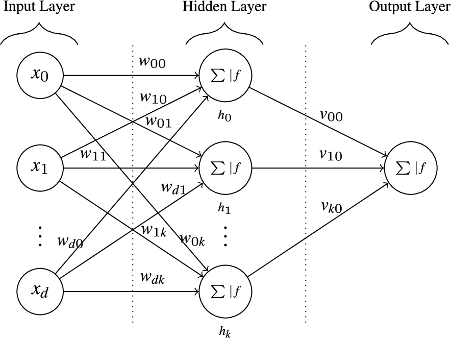
Multilayer Perceptron with d input neurons and one output neuron.

In the present work the individual MLPs in the network layer are trained using one vs. all training. Effectively, the training of the ith MLP is such that the single neuron in the output layer of the MLP is activated only if the MLP recognizes the sample as belonging to the ith class. In other words, the output from the ith MLP is one if the sample belongs to the ith class and is zero otherwise. In a way, these MLPs are binary classifiers because either they know the pattern or they do not know the pattern. It may be noted that the one vs. all training strategy allows us to train each MLP independently of the others. The ith MLP effectively learns a decision boundary that encloses the samples of the ith class seen so far. However, as will be shown later, the actual decision boundaries learnt by the MLPs may not be the ideal one and some MLPs may learn open decision boundaries.

The Monitor perceptron accepts the input from the output layer neuron of each MLP. As noted earlier, each MLP can output only 1 (if it recognizes the sample) or 0 (if it does not recognize the sample). As mentioned in Section 1, the role of the monitor perceptron is to decide whether the sample belongs to one of the known classes or whether it belongs to a new class. In order to make this decision the monitor perceptron first computes a summation of all its inputs. The following conditions hold for the summation:

The summation will be equal to zero if no MLP in the network layer recognizes the sample.

The summation will be equal to one if exactly one MLP in the network layer recognizes it.

Lastly, the summation will be greater than one if more than one MLP in the network layer recognizes the sample.

Thus, a summation value of one indicates that the sample belongs to one of the known classes and other values indicate that the sample belongs to a new class. Thus, based on the value of the summation, the monitor perceptron is able to take its decision. The above logic can be encapsulated by the activation function given by Eqn. (2). The actual decision region can be visualized in Fig. 6. $\begin{matrix} (2) & f (s) = \{\begin{matrix} 1, & \forall s \in 1 \pm ϵ \\ 0, & otherwise \end{matrix} \end{matrix}$

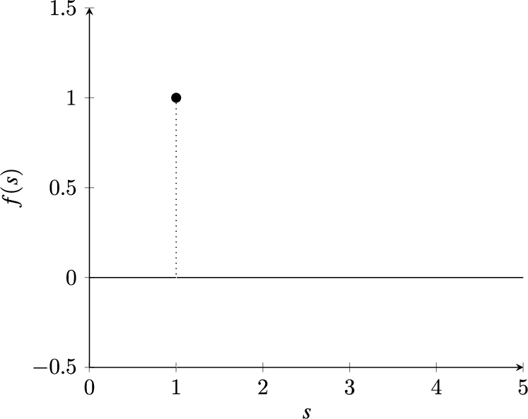
Where ϵ is nearly equal to zero and s is the sum of all inputs. It simply states that the monitor perceptron gets activated if the sum is near to one. Otherwise it does not get activated. In order to understand the rationale of the activation function of the monitor perceptron we observe that the sum, ‘s’, in the above equation can be 0, 1 or $> 1$ . These values will occur on the following conditions:

Fig. 6.

Decision region given by equation (2).

$s = 0$ if none of the MLPs recognize the sample,

$s = 1$ if exactly one MLP recognizes the sample,

$s > 1$ if more than one MLPs recognizes the sample.

The first condition (i.e. $s = 0$ ) implies that the sample belongs to a class that has not been learnt by INNAMP till now. In this case INNAMP has to start the process of learning the samples of the new class which will be described later in this section. The second condition (i.e. $s = 1$ ) implies that the sample belongs to one of the classes that INNAMP has already learnt. We will get $s = 1$ only if exactly one MLP gets activated and it is clear that in this case the sample belongs to the class for which this MLP was dedicated i.e. the sample belongs to one of the known classes. In this case the correct class label needs to be output by INNAMP. This task is handled by the output layer and will be described later when we describe the output layer. The third condition (i.e. $s > 1$ ) usually implies a case of misclassification since more than one MLP recognizes the sample.

The logic of the activation function for the monitor perceptron (Eqn. (2)) is that this special perceptron will get activated only if INNAMP sees a sample of a class that it has not learnt yet. In other words, it is a perceptron that will say “I don’t know” when INNAMP is presented with a sample of a class that it has not learnt. Otherwise this special perceptron will not get activated i.e. it will remain silent. An important point to be noted at this stage is that the logic of the monitor perceptron is independent of the number of classes learnt by INNAMP. Thus, we can add any number of classes but we do not have to retrain the monitor perceptron. In fact, since the logic of the monitor perceptron is fixed, we may “hardwire” it from the beginning. This is crucial because it gives scalability to the architecture and helps resolve the stability-plasticity dilemma.

The Output layer contains $M + 1$ number of neurons corresponding to M number of classes and one additional neuron for new classes. The ith neuron ( $1 ⩽ i ⩽ M$ ) takes two inputs. The first is from the ith MLP and the second is from the monitor neuron. The logic of the neurons in the output layer is again fixed and can be “hardwired” from the beginning. If the INNAMP has been trained for M classes, then the first M neurons of the output layer works as AND gates. Thus, the activation function for the first M neurons of the output layer can be depicted as Eqn. (3) $\begin{matrix} (3) & f (s) = \{\begin{matrix} 1, & s = 2 \\ 0, & s < 2 \end{matrix} \end{matrix}$

The rationale for the above activation function is that the ith output layer neuron is activated if the ith MLP is activated and no other MLP is activated.

Apart from the first M neurons corresponding to the M classes that have been learnt by INNAMP, the output layer consists of one additional neuron that will get activated for samples belonging to new classes i.e. classes that have not been learnt yet by INNAMP. This takes a single input from the monitor perceptron and works as a NOT gate. It may be recalled that the monitor perceptron gives an output of 0 when it gets a sample of a new class. Thus, the NOT function will convert the 0 into a 1. In other words, the $(M + 1)$ th neuron of the output layer gets activated when INNAMP sees a sample from a class that it has not learnt so far. The activation function of this neuron is given by Eqn. (4). $\begin{matrix} (4) & f (s) = \{\begin{matrix} 1, & s = 0 \\ 0, & s = 1 \end{matrix} \end{matrix}$

In effect, only one of the neurons of the output layer can get activated by a particular sample. If one of the first M neurons get activated then we have a sample from a known class. On the other hand, if the last neuron gets activated then we have a sample from a previously unseen class. In such situations we have to extend our network to learn this new class. The flow diagram of INNAMP is presented in Fig. 7.

Fig. 7.

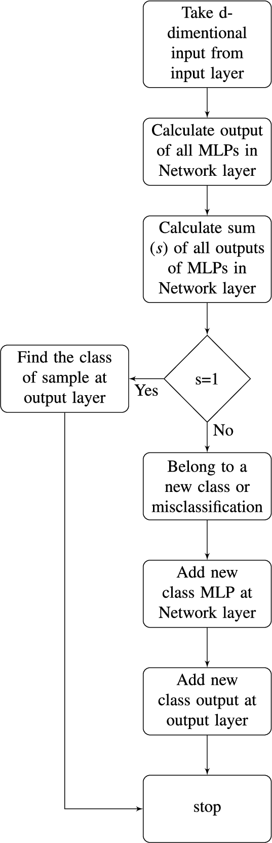
Flow diagram of INNAMP.

We shall now proceed to describe the process of extending the network when INNAMP encounters a sample from a previously unseen class. The first step is to add a new MLP in the network layer, corresponding to the new class. This MLP is again trained using a one vs. all strategy which does not affect the rest of the network. Before training a new MLP we wait for new class samples. Unless these new class samples crosses certain limit we wait. Then we merge these samples to old data set and perform the training of new MLP.

The second step is to add a new neuron in the output layer corresponding to the new class. Since the logic for these neurons is fixed, so no additional training is required for this neuron. No further additions are required in the network. Thus, we see that our architecture allows for a very controlled expansion of the network. In fact, the growth is linear with respect to the number of classes because whenever we add a new class we add a new MLP of fixed size in network layer. Therefore, for every increment in the number of classes we add the same number of neurons in the network.

It is possible that some of the existing MLPs in the network layer may also get activated by the samples from the new class. Therefore, as a third step, we test the MLPs of the existing classes with the new data to check whether they get activated. In case the ith MLP is not activated, then we do not have to perform any retraining of this existing MLP. However, in case the ith MLP is activated, then we have to perform a retraining of this MLP and this is the point where we have to tackle the stability-plasticity dilemma. The retraining will have to be performed using the new and old data. This problem occurs primarily due to poor training of the existing MLPs and can be solved by fine tuning the decision regions learnt by those MLPs.

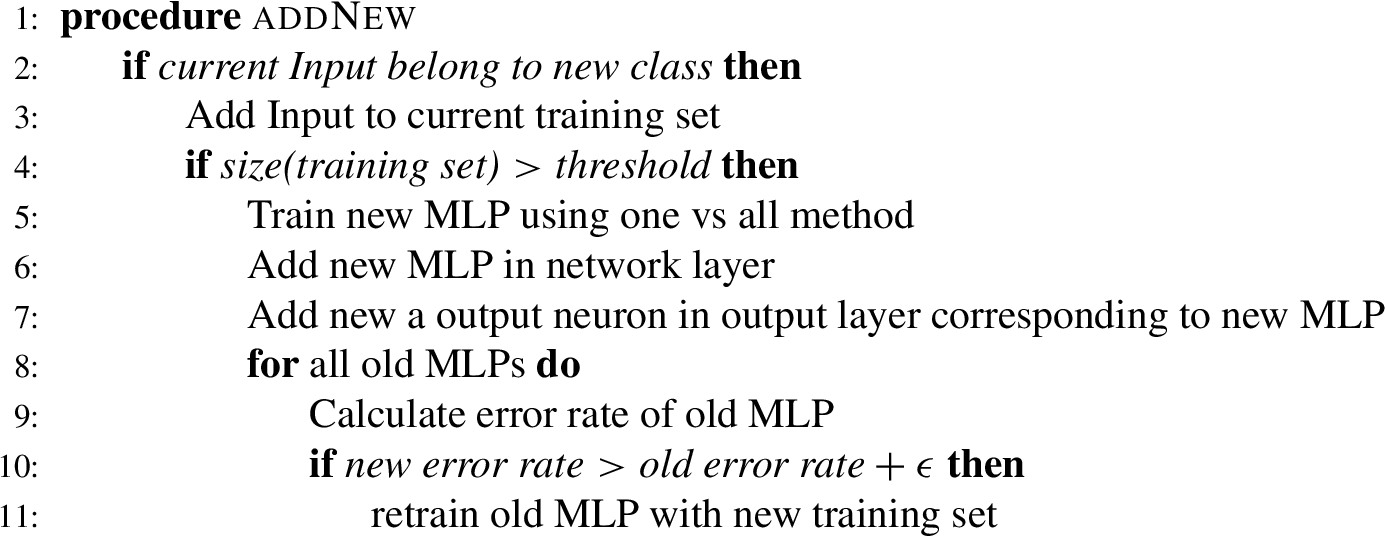
At this stage we should note that each MLP had learnt a decision boundary that enclosed the samples of its class. It is intuitively clear that even after retraining we will not get a significant shift in the decision boundary i.e. the decision boundary will shift only marginally. Based on this hypothesis we retrain these networks such that the initial estimates of the weights, for the purpose of retraining, are the same as the weights that the MLP has already learnt. In practice, we find that only a few epochs of retraining are required to complete the process of adaptation. After the retraining we update these MLPs with the new weights and add the MLP corresponding to the new class in the architecture along with a corresponding neuron in the output layer. In Algorithm 1 below we have summarized the process to be followed when we extend INNAMP for accommodating samples from a new class.

Algorithm 1

Add New Class

It is pertinent to note that this architecture also allows removal of classes. Removal of an old class can be done by simply removing the corresponding MLP from the network layer and the corresponding neuron from output layer, leaving the rest of the architecture unchanged.

As can be seen from the above discussion, the proposed architecture allows for expansion of the network in a controlled manner and can be expanded for any number of classes. It is easy to add a new class and remove or update an existing class without disturbing other classes. Adding a new class implies adding a new MLP in the second layer and a single neuron in the fourth layer. We may also have to make small adaptations in the existing MLPs of the second layer. This would be required only for those existing classes whose decision region encloses samples of the new class.

4. Experiments and results

A series of experiments have been performed to validate the proposed architecture. These experiments were conducted using benchmark data sets taken from UCI machine learning repository [25] and additional data sets, WebKB-41

¹
http://www.inf.ufes.br/~elias/reduzed-WebKB-4-and-Reuters-8.zip

and chars74k [15]. Table 1 presents a summary of all the data sets together with information about the number of classes, number of attributes and number of instances. It may be noted that these are the same data sets as used in an earlier work [11] except chars74k.

Table 1

Details of data sets used in the experiment

	Number of

Data set name	Classes	Attributes	Instances
IRIS	3	4	150
Heart	2	13	270
Spambase	2	57	4601
Car	4	6	1728
WebKB-4	4	3000	4199
CNAE-9	9	856	1080
Chars74K	62	784	74088

These data sets differ in number of classes (2–62) and number of attributes (4–3000). Thus, the chosen data sets will provide a rigorous test of the proposed architecture. In particular, we will be able to examine whether the proposed architecture works when we have a very high number of attributes and classes. Number of attributes of WebKB-4 data set is reduced from 8565 to 3000 as stated in Ciarelli, Oliveira, Salles, 2012 [11].

In order to verify the efficacy of the proposed method we have compared our results with three existing techniques for incremental learning namely the results from Ciarelli, Oliveira, Salles, 2012 [11], the results obtained with fuzzy ARTMAP [9]2

http://www.cns.bu.edu/~artmap/#Carpenter1998b

and the results of Cascade network. Training parameters used for fuzzy ARTMAP are the default values set in the package i.e. training rate (β) is one (

β = 1

); choice parameter (α) is congruent to zero (

α ≅ 0

); the baseline vigilance parameter (ρ) is zero (

ρ_{a} = 0

); the vigilance parameter (

ρ_{a b}

and

ρ_{b}

) is 0.99. We train and test all three networks (fuzzy ARTMAP, Cascade network and INNAMP) with same training and testing set.

Table 2

Results for unseen class data on different data sets

		Seen Class Data				Unseen Class Data

			Correctly Classify				Correctly Classify

Data set name		Size	ARTMAP	Cascade	INNAMP	Size	ARTMAP	Cascade	INNAMP
Car	Train data	1331	1080 ± 7	1280 ± 12	1306 ± 20	52	0	0	19 ± 4
Car	Test data	332	270 ± 7	318 ± 2	318 ± 9	13	0	0	6 ± 4
WebKB-4	Train data	2615	1299 ± 410	1974 ± 121	2315 ± 120	744	0	0	270 ± 48
WebKB-4	Test data	654	258 ± 70	231 ± 31	515 ± 19	186	0	0	63 ± 15
CNAE-9	Train data	480	455 ± 11	377 ± 35	475 ± 3	384	0	0	210 ± 28
CNAE-9	Test data	120	104 ± 3	59 ± 8	108 ± 5	96	0	0	53 ± 9
Chars74k	Train data	54374	29063 ± 723	3364 ± 226	46398 ± 596	12306	0	0	4105 ± 218
Chars74k	Test data	6041	2896 ± 124	332 ± 18	4733 ± 79	1367	0	0	453 ± 32

Table 3

Average performance of the full system on data sets where class count is less than or equal to three (values in percentage)

data set	Training	Testing
IRIS	$97.66 \pm 1.16$	$97.00 \pm 4.83$
Heart	$84.60 \pm 1.69$	$77.03 \pm 9.03$
Spambase	$98.69 \pm 0.11$	$98.39 \pm 0.68$

The results obtained for all the data sets are given in Tables 2, 3, 4 and 5. Moreover, we also perform 10-fold cross validation on each data set to verify the correctness of our architecture. We also perform 10-fold cross validation among the arrival of new class data by changing the set of initial classes and arrival of samples of new classes. This additional test has been performed so that we can test whether the architecture is sensitive to the order of arrival of data.

Table 4

Average performance of the full system on data sets with more than three classes (values in percentage)

Method	Training	Testing
Car
ePNN (Ciarelli et al., 2012)	80.99 ± 1.99	81.13 ± 2.68
IPNN	69.92 ± 1.49	71.41 ± 2.85
EFuNN	92.18 ± 2.58	82.28 ± 1.91
ePNN (Ciarelli et al., 2010)	73.00 ± 5.96	71.62 ± 8.98
MLP	84.56 ± 4.07	78.78 ± 20.73
GMM	67.12 ± 5.35	67.34 ± 6.19
fuzzy ARTMAP	80.26 ± 0.35	81.18 ± 3.03
Cascade	34.35 ± 7.69	35.18 ± 6.55
INNAMP	92.93 ± 7.31	91.16 ± 5.28
WEBKB-4
ePNN (Ciarelli et al., 2012)	84.68 ± 9.59	77.70 ± 10.30
IPNN	99.47 ± 0.17	61.97 ± 4.35
EFuNN	78.29 ± 7.05	58.05 ± 9.23
ePNN (Ciarelli et al., 2010)	86.08 ± 3.15	78.45 ± 4.31
MLP	95.54 ± 2.41	87.00 ± 2.40
GMM	52.94 ± 5.64	52.58 ± 6.01
fuzzy ARTMAP	32.87 ± 4.18	28.93 ± 4.15
Cascade	20.48 ± 0.10	23.85 ± 1.2
INNAMP	86.61 ± 1.77	77.56 ± 1.77
CNAE-9
ePNN (Ciarelli et al., 2012)	96.64 ± 1.89	88.94 ± 3.54
IPNN	99.90 ± 0.27	85.56 ± 3.18
EFuNN	67.97 ± 5.71	65.07 ± 6.01
ePNN (Ciarelli et al., 2010)	95.91 ± 2.12	88.06 ± 3.21
MLP	99.60 ± 0.49	92.35 ± 2.69
GMM	27.94 ± 18.58	22.48 ± 16.66
fuzzy ARTMAP	95.072 ± 1.27	86.20 ± 2.97
Cascade	10.90 ± 0.44	11.02 ± 1.11
INNAMP (50)	90.50 ± 4.45	81.29 ± 4.24

Table 5

Average performance on Chars74K data set (values in percentage)

Method	Accuracy
$GB + NN$	54.03
$HoG + NN$	58
ABBYY FineReader	31
$Tensor + NN$	68.5
$Rank-1 Tensor + cross validation$	74
fuzzy ARTMAP	47.93
Cascade	5.49
INNAMP	70.27

The performance of our architecture is presented in terms of average performance across all the folds together with the maximum change in performance from the average. It may be noted that if the class count is smaller than or equal to three then we train all the networks at once because there is no scope for adding new classes incrementally. The results for such cases are presented in Table 3. The results obtained with data sets that have more than three classes are presented in Tables 2, 4 and 5. The incremental learning process described earlier is applied only to these data sets.

Fig. 8.

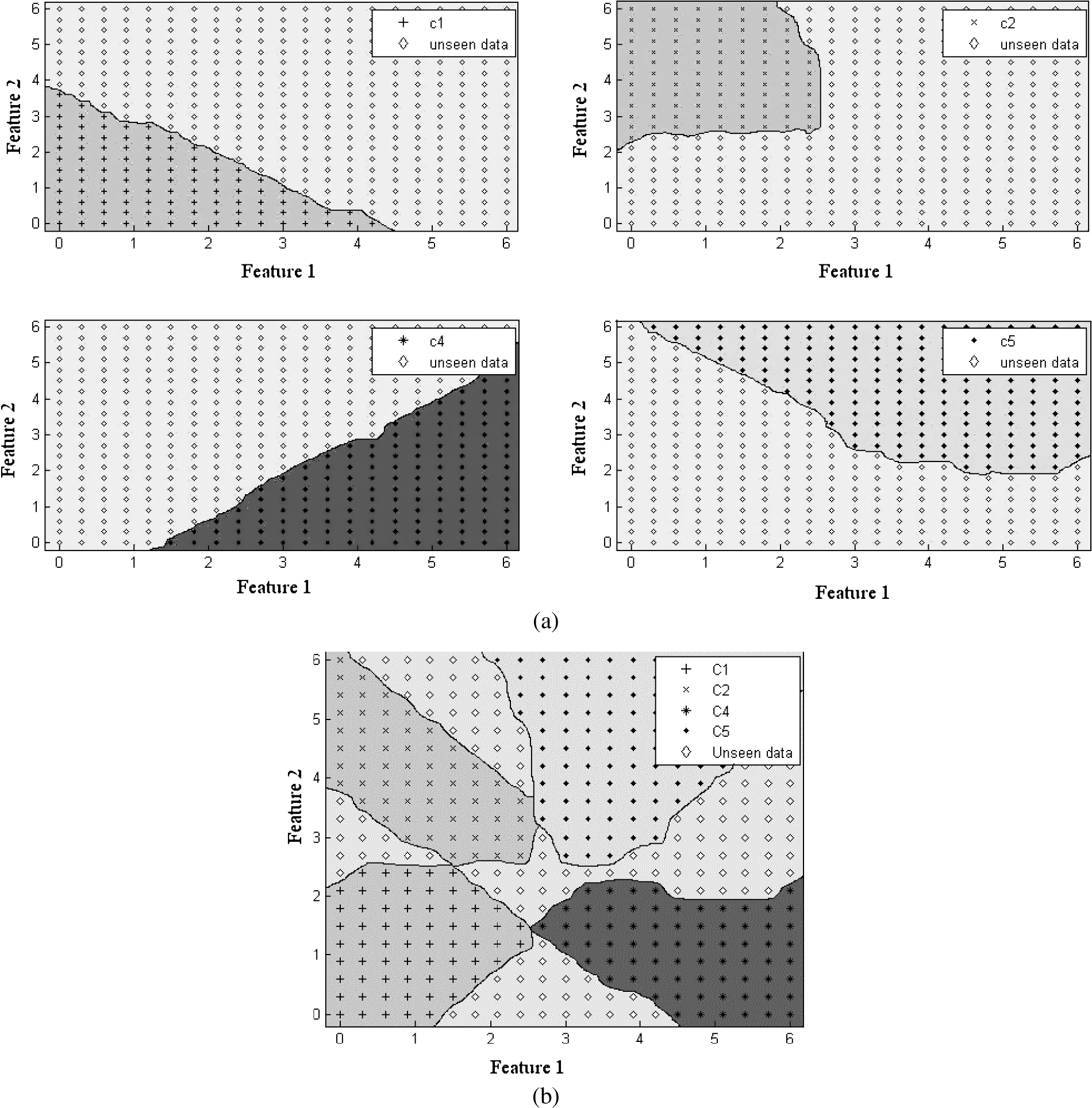
(a) Class boundaries for individual classes C1, C2, C4 and C5; (b) Resultant decision regions for all four classes.

If the class count is larger than three then we first train with half plus one classes initially. Therefore, for Car, WebKB-4 and CNAE-9 we started with 3, 3 and 5 classes initially. In the case of chars74k data set we take 50 classes as the starting point. The remaining classes were added incrementally using the process described in the previous section. After the initial training, we test the system with data from the seen and unseen classes. The performances of the networks for these four data sets are shown in Table 2.

It is clear from Table 2 that classifiers like ARTMAP and Cascade run in two modes i.e. training and testing. Moreover, if they are running on training mode then they can accommodate new data and new class. However, the story is quite different when they are running in testing mode. In the testing mode these networks take a sample and they always classify that sample into one of the existing class. In other words, these techniques can say “I don’t know” only in the training mode and not in the testing mode. In this respect the proposed architecture, INNAMP, works in a different way. In testing mode, when INNAMP sees a sample from an unseen class data it is able to say “I don’t know” and then switch over to the expansion and adaptation as explained in the previous section.

In order to understand the relevance of the numbers we need a few observations. Firstly, we see that our proposed architecture and process does manage to discover the arrival of samples from a class that it has not learnt yet. Moreover, the results are not affected by the ordering of classes i.e. the order of arrival of training data. Moreover, as will be shown subsequently, the overall error rate compares favorably with earlier approaches. However, the error rate for the samples from already learnt classes is significantly lower than that of samples from new classes. This is indicative of poor training. This aspect is analyzed in more detail in the following.

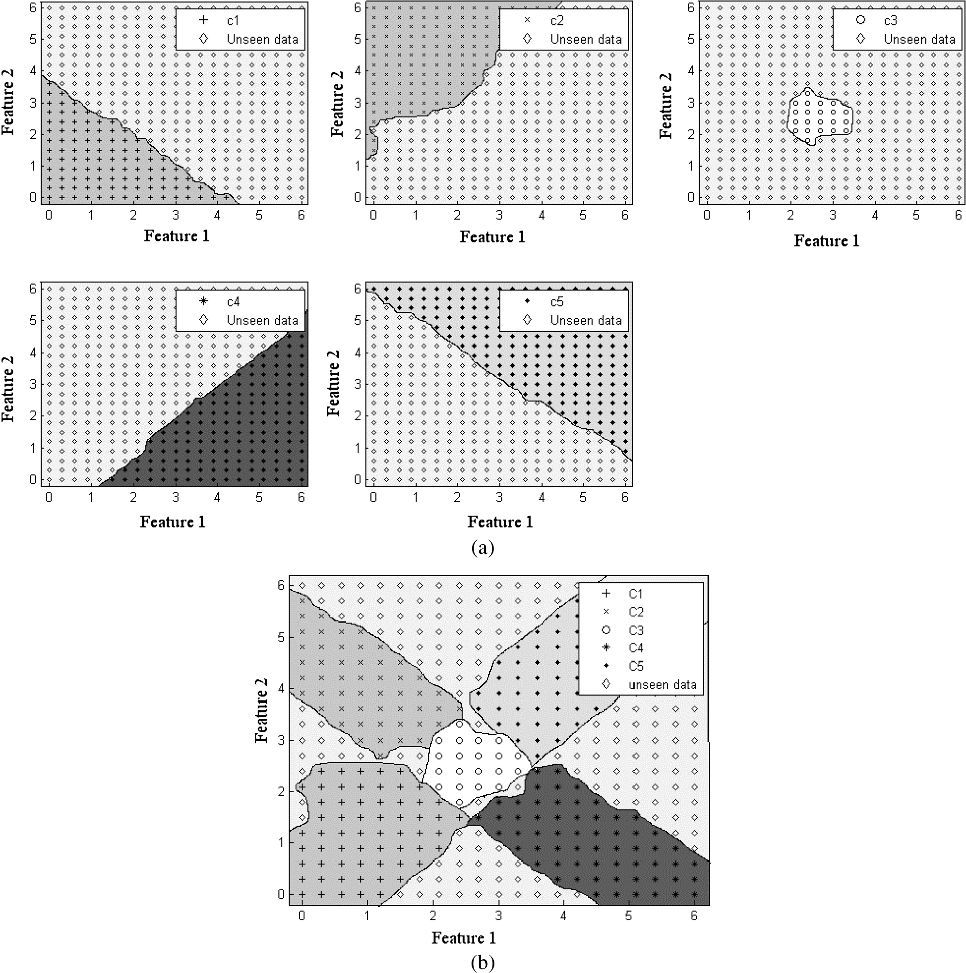
We again consider the example given in the introduction to understand the error rate for unseen data. We train INNAMP with the samples from classes C1, C2, C4 and C5 of Fig. 1. The class boundaries for network layer of INNAMP for different classes are shown in Fig. 8(a), where the dark region denotes the seen data region and light region is for the unseen data region for that particular class.

Now when we combine all these classifiers for output layer of INNAMP, the final decision regions are shown in Fig. 8(b). The first point to be noted is that certain portions of the feature space remain available for unseen data which, in this example, is the data from C3. This result is in stark contrast to the case where we train an MLP using the samples from C1, C2, C4 and C5 which was shown in Fig. 3 which did not have any region for unseen data. Thus, while our architecture and approach does create a decision region for the as yet un-learnt class, we can see that the already learnt classes are occupying decision regions in excess of what they actually require leading to misclassifications of samples from C3.

Now when we test the above architecture with samples of class C3, then some of samples are correctly recognized as unseen data while other samples of C3 are wrongly classified into one of the existing classes. This is depicted in Fig. 9 where the diamond sign represents the samples of C3 that are correctly classified as belonging to an unseen class. This situation is better than training a single MLP for all the four classes (C1, C2, C4 and C5) because such an MLP would have misclassified all samples of C3.

Fig. 9.

Results of architecture with unseen and seen data.

Once we get sufficient number of samples declared as belonging to a new class, we run through the procedure described above for adding a new class. The number of samples may be decided as the minimum number of samples of a previously trained class or some other heuristic. The final decision boundaries of separate MLPs and decision regions are shown in Fig. 10(a) and Fig. 10(b) respectively. The latter figure clearly shows that a new decision region has been created for the samples of the newly arrived class.

The final results obtained using our method is given in Table 4 for Car, WebKB-4 and CNAE-9 benchmark data sets. We have also included the results by Ciarelli, Oliveira, and Salles on the same data sets [11] for the purpose of comparison. We have also included the results obtained using other methods like Evolving Probabilistic Neural Network (ePNN), Incremental Probabilistic Neural Network (IPNN), Evolving Fuzzy Neural Network (EFuNN), Multilayer Perceptron (MLP) Gaussian Mixture Model (GMM), ARTMAP and Cascade network. As can be observed from this table, our method is comparable to or outperforms all these methods.

Table 5 shows the performance of INNAMP on Chars74K data set. We simply take all the 74k (computer fonts, handwritten and natural scenes). We first binarize the natural scenes images, then crop all the images from all the sides so that only the character remains in the image. Cropped images are then resized to $28 \times 28$ pixels. These images are directly used for training the networks and no effort was expended on noise removal or feature extraction. A comparison of our result with previously used methods on the same data set [3] shows that only one of the methods outperforms INNAMP and this method uses a sophisticated feature extraction technique.

Fig. 10.

(a) Separate regions of all MLP’s using all 5 classes, (b) Final decision boundaries using INNAMP.

Figure 11(a) and 11(b) shows the performance of INNAMP with respect to class increment for CNAE-9 and Chars74K during training and testing phases. It is very clear from the figure that if the number of classes increase there is slight decrement in the performance of INNAMP. This is due to the overlap in the class boundaries due to training of separate MLPs as shown in the above example. It is clear from these results that if we get tighter boundaries while training the individual networks then we can improve the performance of INNAMP. Ideal decision boundary for a class would be that boundary which encloses the outermost data points of that class. This would leave more regions for accommodating samples of a new class and thus increase the accuracy.

In case of fuzzy ARTMAP we have to initially define the number of classes for which we are going to train our network. If the class count goes above that then we have to create a new network and retrain it. In other words, we need to have an estimate of the total number of classes that the network will ultimately recognize. ARTMAP does not have a mechanism to keep adding new classes. On the other hand, there is no need to define the number of classes in case of INNAMP because we can add any number of classes by simply adding one more MLP for a new class.

In terms of growth of network ARTMAP has a fixed size and there is no necessity of adding new neurons because the maximum number of classes is available a priori. On the other hand, Cascade Correlation Network and Evolving Fuzzy Neural Network (EFuNN) allows the network to grow but the growth is uncontrolled. In the cases of Probabilistic Neural Network (ePNN) and Incremental Probabilistic Neural Network (IPNN) the growth of network depends on the number of training samples because there is a neuron for each training data. For example if your data set contains 10000 training samples then there is 10000 neurons along with one neuron for each class and one output neuron. Thus, for these latter cases, when we add a sample from a new class then we also have to add a neuron into the network. This leads to very large networks and high computational complexity.

In contrast to other models of incremental learning, the growth of network in INNAMP is linear in the number of classes. As explained in the previous section, for each class we need to add one MLP in the second layer and a single neuron in the fourth layer. Thus, the rate of growth depends upon the size of MLP in network layer. If an MLP has one hidden layer with, say, 10 neurons and there is 1 neuron in the output layer of the MLP, then the total number of neurons in each MLP is 11. Moreover, there is one neuron in the output layer of INNAMP for every MLP. Thus, for adding one class we require 12 neurons in the network. We have performed all our experiments using the above architecture. However, the size of the MLPs can change with the data set but we will still require only one MLP per class. The above shows that while our architecture can accommodate an arbitrary number of classes (unlike ARTMAP), the corresponding growth in the network is very controlled.

Fig. 11.

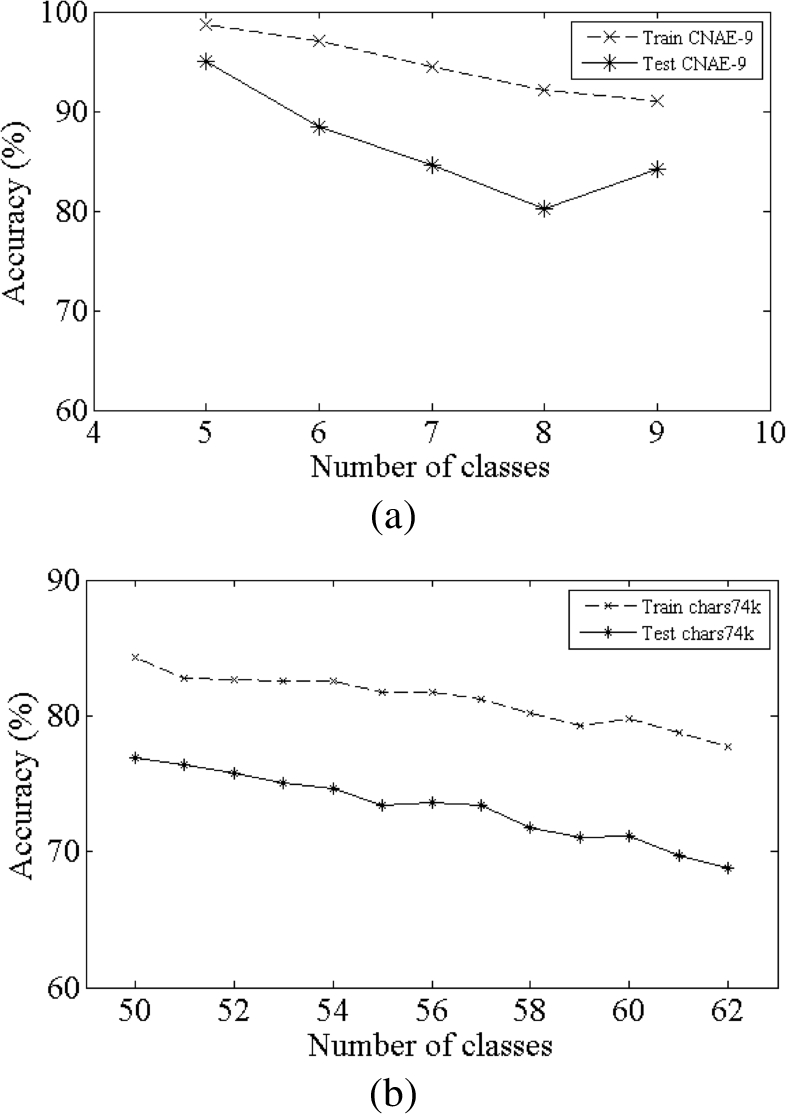
(a) Change in accuracy as number of classes increases for CNAE-9 data set (b) Change in accuracy as number of classes increases for Char74K.

5. Conclusions and future work

This paper presents INNAMP, which is an incremental neural network architecture, with monitor perceptron, using parallel multilayer perceptron networks. The main advantage of this architecture is that the monitor perceptron is able to differentiate between samples from seen (i.e. already learnt) and unseen (i.e. not-yet learnt) classes. The system grows as the number of classes increase but it is a controlled growth. The network grows linearly with the increase in number of classes. Moreover, the retraining required when a sample of an unknown class is presented represents a nice balance between stability and plasticity. A major difference between the proposed approach and earlier approaches like ARTMAP is that we do not have to adjust or fine tune any parameter. As explained in the previous section, the network is able to recognize the arrival of samples from a new class. In case samples from new classes arrive then the system expands and adapts to the changes in a controlled fashion.

A series of experiments have been performed on public domain data sets with INNAMP and results are comparable with other techniques that include both incremental and non-incremental methods. Therefore, it appears that IANNMP is an effective alternative to the existing incremental neural architectures.

A matter of concern with the present architecture is that while it will work well for classes that are well separated in the feature space, the monitor perceptron may not be able to take correct decisions if there is a strong overlap between the new (unseen) class and one of the existing (known) classes. This is a possible scenario when the number of classes becomes very large. A possible solution to this problem is that we can replace the single monitor perceptron with a full-fledged network that can learn more complex decision boundaries instead of the simple decision boundary learnt by the single perceptron. We can allow each MLP in the network layer to output a probability of a particular sample for belonging to a certain class. These probabilities are then given to the decision layer for determining whether the sample belongs to one of the known classes or whether the sample belongs to a new class.

The other problem with this architecture is open decision regions of some classes. If a sample from a new class lies in one of these regions, then the system classifies this sample wrongly. To overcome this problem we have to create alternative methods of training that can lead to closed decision boundaries that encloses the samples of known classes more tightly. If we succeed in creating closed boundaries that are tight then we do not have to retrain the network while adding the new classes.

Footnotes

Acknowledgement

The authors gratefully acknowledge the infrastructural support provided by Indian Institute of Information Technology, Allahabad (IIIT-A). One of the authors (SG) also acknowledges the financial support from IIIT-A.

References

Al-Daoud, Incremental learning of auto-association multilayer perceptrons network, Int. Arab J. Inf. Technol. 3(1) (2006), 16–19.

Al-Daraiseh,

Kaylani,

Georgiopoulos,

Mollaghasemi,

A.S.

Wu and

Anagnostopoulos, GFAM: Evolving fuzzy ARTMAP neural networks, Neural Networks 20(8) (2007), 874–892. doi:10.1016/j.neunet.2007.05.006.

Ali and

Foroosh, Character recognition in natural scene images using rank-1 tensor decomposition, in: 2016 IEEE International Conference on Image Processing, ICIP 2016, Phoenix, AZ, USA, September 25–28, 2016, pp. 2891–2895. doi:10.1109/ICIP.2016.7532888.

G.C.

Anagnostopoulos and

Georgiopoulos, Ellipsoid ART and ARTMAP for incremental unsupervised and supervised learning, in: Proc. SPIE 4390, Applications and Science of Computational Intelligence IV, Vol. 4390, 2001, pp. 293–304. doi:10.1117/12.421180.

Aran and

Alpaydin, An incremental neural network construction algorithm for training multilayer perceptron, 2003.

Bhattacharyya,

Metla,

Bandyopadhyay,

Tudu and

Jana, Incremental PNN classifier for a versatile electronic nose, in: 2008 3rd International Conference on Sensing Technology, Nov. 2008, pp. 242–247. doi:10.1109/ICSENST.2008.4757106.

Boujelbene and

Zribi, The neural networks with an incremental learning algorithm approach for mass classification in breast cancer, Biomedical Data Mining 5 (2016), 118. doi:10.4172/2090-4924.1000118.

J.L.

Calvo-Rolle,

Fontenla-Romero,

Pérez-Sánchez and

Guijarro-Berdiòas, Adaptive inverse control using an online learning algorithm for neural networks, Informatica 25(3) (2014), 401–414. doi:10.15388/Informatica.2014.20.

G.A.

Carpenter,

Grossberg,

Markuzon,

J.H.

Reynolds and

D.B.

Rosen, Fuzzy ARTMAP: A neural network architecture for incremental supervised learning of analog multidimensional maps, IEEE Transactions on Neural Networks 3(5) (1992), 698–713. doi:10.1109/72.159059.

10.

G.A.

Carpenter,

Grossberg and

J.H.

Reynolds, ARTMAP: Supervised real-time learning and classification of nonstationary data by a self-organizing neural network, Neural Networks 4(5) (1991), 565–588. doi:10.1016/0893-6080(91)90012-T.

11.

P.M.

Ciarelli,

Oliveira and

E.O.T.

Salles, An incremental neural network with a reduced architecture, Neural Networks 35 (2012), 70–81. doi:10.1016/j.neunet.2012.08.003.

12.

P.M.

Ciarelli,

E.O.T.

Salles and

Oliveira, An evolving system based on probabilistic neural network, in: 2010 Eleventh Brazilian Symposium on Neural Networks, Oct. 2010, pp. 182–187. doi:10.1109/SBRN.2010.39.

13.

J.F.

Connolly,

Granger and

Sabourin, Incremental adaptation of fuzzy ARTMAP neural networks for video-based face classification, in: 2009 IEEE Symposium on Computational Intelligence for Security and Defense Applications, July 2009, pp. 1–8. doi:10.1109/CISDA.2009.5356545.

14.

Cruz-Vega and

H.J.

Escalante, An online and incremental GRLVQ algorithm for prototype generation based on granular computing, Soft Computing (2016), 1–14. doi:10.1007/s00500-016-2042-0.

15.

T.E.

De Campos,

B.R.

Babu and

Varma, Character recognition in natural images, 2009.

16.

R.O.

Duda,

P.E.

Hart and

D.G.

Stork, Pattern Classification, 2nd edn, Wiley-Interscience, 2000. ISBN 0471056693.

17.

S.E.

Fahlman and

Lebiere, The cascade-correlation learning architecture, in: Advances in Neural Information Processing Systems, Vol. 2,

D.S.

Touretzky, ed., Morgan Kaufmann Publishers Inc., San Francisco, CA, USA, 1990, pp. 524–532. ISBN 1-55860-100-7.

18.

Frean, The upstart algorithm: A method for constructing and training feedforward neural networks, Neural Comput. 2(2) (1990), 198–209. doi:10.1162/neco.1990.2.2.198.

19.

Gepperth and

Hammer, Incremental learning algorithms and applications, in: European Sympoisum on Artificial Neural Networks (ESANN), 2016.

20.

J.B.

Gomm, Adaptive neural network approach to on-line learning for process fault diagnosis, Transactions of the Institute of Measurement and Control 20(3) (1998), 144–152. doi:10.1177/014233129802000305.

21.

Grossberg, Competitive learning: From interactive activation to adaptive resonance, Cognitive Science 11 (1987), 23–63. doi:10.1111/j.1551-6708.1987.tb00862.x.

22.

F.H.

Hamker, Life-long learning cell structures – Continuously learning without catastrophic interference, Neural Networks 14(4–5) (2001), 551–573. doi:10.1016/S0893-6080(01)00018-1.

23.

G.-B.

Huang and

Chen, Letters: Convex incremental extreme learning machine, Neurocomput. 70(16–18) (2007), 3056–3062. doi:10.1016/j.neucom.2007.02.009.

24.

Kohonen, Improved versions of learning vector quantization, in: 1990 IJCNN International Joint Conference on Neural Networks, Vol. 1, June 1990, pp. 545–550. doi:10.1109/IJCNN.1990.137622.

25.

Lichman, UCI Machine Learning Repository, University of California, Irvine, School of Information and Computer Sciences, 2013, http://archive.ics.uci.edu/ml.

26.

Mandziuk and

Shastri, Incremental class learning approach and its application to handwritten digit recognition, Inf. Sci. 141(3–4) (2002), 193–217. doi:10.1016/S0020-0255(02)00170-6.

27.

Y.L.

Murphey,

Z.H.

Chen and

L.A.

Feldkamp, An incremental neural learning framework and its application to vehicle diagnostics, Applied Intelligence 28(1) (2008), 29–49. doi:10.1007/s10489-007-0040-8.

28.

Polikar,

Upda,

S.S.

Upda and

Honavar, Learn++: An incremental learning algorithm for supervised neural networks, IEEE Transactions on Systems, Man, and Cybernetics, Part C (Applications and Reviews) 31(4) (2001), 497–508. doi:10.1109/5326.983933.

29.

Pratama,

Lu,

Anavatti,

Lughofer and

C.-P.

Lim, An incremental meta-cognitive-based scaffolding fuzzy neural network, Neurocomputing 171 (2016), 89–105. doi:10.1016/j.neucom.2015.06.022.

30.

Read,

Bifet,

Pfahringer and

Holmes, Batch-incremental versus instance-incremental learning in dynamic and evolving data, in: Proceedings of the 11th International Conference on Advances in Intelligent Data Analysis, IDA’12, Springer-Verlag, Berlin, Heidelberg, 2012, pp. 313–323. ISBN 978-3-642-34155-7. doi:10.1007/978-3-642-34156-4_29.

31.

Seera and

C.P.

Lim, Transfer learning using the online fuzzy min–max neural network, Neural Computing and Applications 25(2) (2014), 469–480. doi:10.1007/s00521-013-1517-5.

32.

Seipone and

J.A.

Bullinaria, Evolving improved incremental learning schemes for neural network systems, in: Proceedings of the IEEE Congress on Evolutionary Computation, CEC 2005, Edinburgh, UK, 2–4 September 2005, pp. 2002–2009. doi:10.1109/CEC.2005.1554941.

33.

Shen and

Hasegawa, A fast nearest neighbor classifier based on self-organizing incremental neural network, Neural Netw. 21(10) (2008), 1537–1547. doi:10.1016/j.neunet.2008.07.001.

34.

Shiotani,

Fukuda and

Shibata, A neural network architecture for incremental learning, Neurocomputing 9(2) (1995), 111–130, Control and Robotics, Part {II}. doi:10.1016/0925-2312(94)00061-V.

35.

D.F.

Specht, Probabilistic neural networks, Neural Netw. 3(1) (1990), 109–118. doi:10.1016/0893-6080(90)90049-Q.

36.

Tzikas and

Likas, An incremental Bayesian approach for training multilayer perceptrons, in: Artificial Neural Networks – ICANN 2010 – 20th International Conference, Proceedings, Part I, Thessaloniki, Greece, September 15–18, 2010, pp. 87–96. doi:10.1007/978-3-642-15819-3_12.

37.

J.H.

Wang and

H.Y.

Wang, Incremental neural network construction for text classification, in: 2014 International Symposium on Computer, Consumer and Control, June 2014, pp. 970–973. doi:10.1109/IS3C.2014.254.

38.

Xu,

Shen and

Zhao, An incremental learning vector quantization algorithm for pattern classification, Neural Computing and Applications 21(6) (2012), 1205–1215. doi:10.1007/s00521-010-0511-4.

39.

Yan,

Jiang,

Zheng,

Peng and

Li, A multilayer perceptron-based medical decision support system for heart disease diagnosis, Expert Syst. Appl. 30(2) (2006), 272–281. doi:10.1016/j.eswa.2005.07.022.

40.

K.S.

Yap,

C.P.

Lim and

Mohamad-Saleh, An enhanced generalized adaptive resonance theory neural network and its application to medical pattern classification, Journal of Intelligent and Fuzzy Systems 21(1–2) (2010), 65–78. doi:10.3233/IFS-2010-0436.

41.

Yen and

Meesad, Pattern classification by an incremental learning fuzzy neural network, in: Neural Networks, 1999. IJCNN ’99. International Joint Conference on, Vol. 5, 1999, pp. 3230–3235. doi:10.1109/IJCNN.1999.836173.

42.

Zurada, Introduction to Artificial Neural Systems, West Publishing Co., St. Paul, MN, USA, 1992. ISBN 0-314-93391-3.

INNAMP: An incremental neural network architecture with monitor perceptron

Abstract

Keywords

1. Introduction

2. Related work

3. Incremental artificial neural network with monitor perceptron

3.1. Motivation for INNAMP

1 http://www.inf.ufes.br/~elias/reduzed-WebKB-4-and-Reuters-8.zip

Footnotes

Acknowledgement

References

¹
http://www.inf.ufes.br/~elias/reduzed-WebKB-4-and-Reuters-8.zip