Multi-agent path finding on real robots

Abstract

The problem of Multi-Agent Path Finding (MAPF) is to find paths for a fixed set of agents from their current locations to some desired locations in such a way that the agents do not collide with each other. This problem has been extensively theoretically studied, frequently using an abstract model, that expects uniform durations of moving primitives and perfect synchronization of agents/robots. In this paper we study the question of how the abstract plans generated by existing MAPF algorithms perform in practice when executed on real robots, namely Ozobots. In particular, we use several abstract models of MAPF, including a robust version and a version that assumes turning of a robot, we translate the abstract plans to sequences of motion primitives executable on Ozobots, and we empirically compare the quality of plan execution (real makespan, the number of collisions).

Keywords

Path planning multi-agent systems real robots

1. Introduction

Multi-agent path finding (MAPF) recently attracted a lot of attention of AI research community. It is a hard problem with practical applicability in areas such as warehousing and games. Frequently, an abstract version of the problem is solved, where a graph defines possible locations (vertices) and movements (edges) of agents and agents move synchronously. At any time, no two agents can stay in the same vertex to prevent collisions so the obtained plans are collision free and hence blindly executable. The plan of each agent consists of move (to a neighboring vertex) and wait (in the same vertex) actions. Makespan and sum-of-cost (plan lengths) are two frequently studied objectives.

In this paper, we focus on answering two questions: how to execute abstract plans obtained from existing MAPF algorithms and models on real robots and how the quality of abstract plans is reflected in the quality of executed plans. The goal is to verify if the abstract plans are practically relevant and, if the answer is no (as expected), to provide feedback to improve abstract models to be closer to reality. We use a fleet of Ozobot Evo robots to perform the plans. These robots provide motion primitives, for example, they can turn left/right, follow a line, and recognize line junction, so it is not necessary to solve classical robotics tasks such as localization. Though the robots have proximity sensors, the plans are executed blindly based on the MAPF setting as the plans should already be collision free.

Specifically, we explore the very classical MAPF setting as described above, the k-robust setting [1], where a gap is required between the robots to compensate possible delays during execution, and finally a model that directly encodes turning operations (the classical setting does not assume direction of movement). The abstract plans are then translated to motion primitives, which consist of forward movement, turning left/right, and waiting. We explore different durations of these primitives to see their effect on robot synchronization. As far as we know this is the first study of practical quality of plans obtained from abstract MAPF models. This paper extends the paper [2] by more systematic evaluation of models using a larger set of maps.

The paper is organized as follows. We will first introduce the abstract MAPF problem formally and survey approaches for its solving. Then we will give more details on why it is important to look at the execution of abstract plans on real robots. After that, we will describe all the models used in this study and how they are translated to executable primitives of Ozobot Evo robots. Finally, we will describe our experimental setting and give results of an empirical evaluation.

2. The MAPF problem

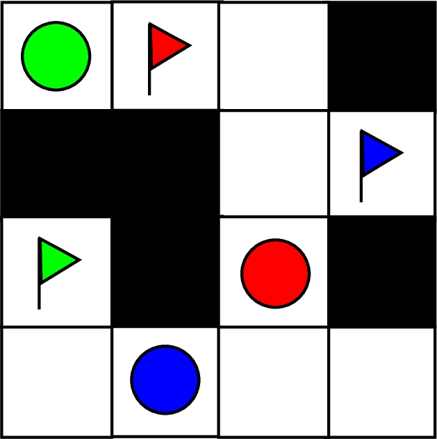
Formally, the MAPF problem is defined by a graph $G = (V, E)$ and a set of agents $a_{1}, \dots, a_{k}$ , where each agent $a_{i}$ is associated with starting location $s_{i} \in V$ and goal location $g_{i} \in V$ . An example of MAPF instance can be seen in Fig. 1. The time is discrete and in every time step each agent can either move from its location to a neighboring location or wait in its current location. A grid map with a unit length of each edge is often used to represent the environment [12]. We will also be using this type of maps in this paper.

Fig. 1.

Example of a MAPF instance. Coloured circles represent agents, while flags represent desired goals.

Let $π_{i} [t]$ denote the location (vertex of graph G) of agent $a_{i}$ at time step t. Plan $π_{i}$ is the sequence of locations for agent $a_{i}$ . The MAPF task is to find a valid plan π that is a union of plans of all agents. We say that π is valid if (i) each agent starts and ends in its starting and goal location respectively, (ii) no two agents occupy the same vertex at the same time, and (iii) no two agents move along the same edge at the same time in opposite directions (they do not swap their positions). Formally this can be written as:

$\forall i : π_{i} [0] = s_{i} \land π_{i} [T] = g_{i}$ , where T is the last time step.

$\forall t, i \neq j : π_{i} [t] \neq π_{j} [t]$

$\forall t, i \neq j : π_{i} [t] \neq π_{j} [t + 1] \lor π_{i} [t + 1] \neq π_{j} [t]$

Note that these constraints allow agents to move on a fully occupied cycle in the graph, as long as the cycle consists of at least three vertices. There are other settings in regards to the allowed movements that are used. The first one requires the vertex an agent wants to enter to be empty before entering (sometimes called pebble motion) [9]. The other allows agent to move into an occupied vertex, provided that the vertex will be empty by the time the agent arrives (this part is the same as the conditions for valid solution we are using in this paper), but forbidding movement on closed cycles [17]. All algorithms presented in this paper can be easily modified to work on either of those settings.

We denote $| π_{i} |$ as the length of plan for agent $a_{i}$ (formally, $| π_{i} | = \min {t | \forall t^{'} ⩾ t : π_{i} [t^{'}] = g_{i}}$ ). Then we can define two objective functions that measure the quality of the found valid plan π. $\begin{array}{l} Makespan (π) = max_{i} | π_{i} | \\ SumOfCost (π) = \sum_{i} | π_{i} | \end{array}$

Both makespan [19] and sum of cost (SoC) [16] are well known and studied in the literature. It can be shown that when we require the solution to be optimal for either of those functions, the problem is NP-hard [11,20]. In this paper, we focus only on makespan-optimal plans.

To solve MAPF optimally, one can generally use algorithms from one of the following categories:

Reduction-based solvers are solvers that reduce MAPF to another known problem such as SAT [18], integer linear programming [21], and answer set programming [6]. These approaches are based on using fast solvers for given formalism and consist mainly of translating MAPF to that formalism.

Search-based solvers include variants of A* over a global search space – all possibilities how to place agents into the vertices of the graph [15]. Other make use of novel search trees [5,13,14] that search over some constraints put on the agents.

Though the plans obtained by different MAPF solvers might be different, the optimal plans are frequently similar and tight (no superfluous steps are used). As solving MAPF is not the topic of this paper (we focus on evaluating the practical relevance of obtained plans), any optimal MAPF solver can be used. We decided for the reduction-based solver implemented in the Picat programming language [4] that uses translation to SAT. This solver has performance comparable to state-of-the-art solvers and has the advantage of easy modification and extension of the core model, for example adding further constraints or using numerical constraints.

The Picat solver (like other reduction-based solvers) follows the planning-as-satisfiability framework [8], where a layered graph is used to encode the plans of a given length. Each layer describes positions of all agents in a given time step. As the plan length is unknown, the number of layers is incrementally increased until a solvable model is obtained. A Boolean variable $B_{t, a, v}$ indicates if agent a ( $a = 1, 2, \dots, k$ ) occupies vertex v ( $v = 1, 2, \dots, n$ ) at time t ( $t = 0, 1, \dots, m$ ). The following constraints ensure the validity of every state and every transition:

Each agent starts and ends in desired location. $\begin{array}{l} B_{0, a, s_{a}} = 1 for a = 1, \dots, k, \\ B_{m, a, g_{a}} = 1 for a = 1, \dots, k . \end{array}$

Each agent occupies exactly one vertex at each time. $\begin{array}{l} \sum_{v = 1}^{n} B_{t, a, v} = 1 \\ for t = 0, \dots, m, and a = 1, \dots, k . \end{array}$

No two agents occupy the same vertex at any time. $\begin{array}{l} \sum_{a = 1}^{k} B_{t, a, v} ⩽ 1 \\ for t = 0, \dots, m, and v = 1, \dots, n . \end{array}$

If agent a occupies vertex v at time t, then a occupies a neighboring vertex at time $t + 1$ (v is assumed to be among neighbors of v). $\begin{array}{l} B_{t, a, v} = 1 \Rightarrow \sum_{u \in neibs (v)} (B_{(t + 1), a, u}) ⩾ 1 \\ for t = 0, \dots, m - 1, a = 1, \dots, k, \\ and v = 1, \dots, n . \end{array}$

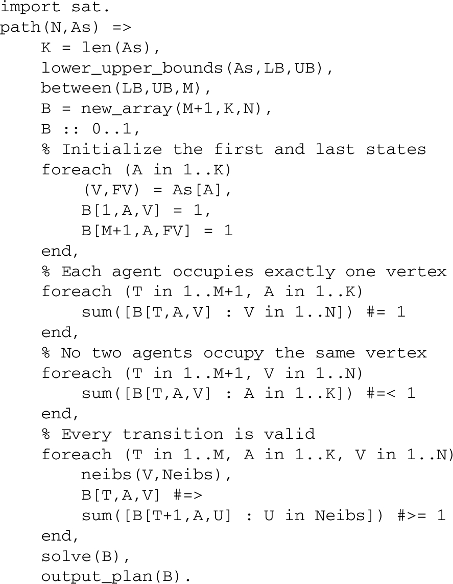
The model consists of $k \times (m + 1) \times n$ Boolean variables, where k is the number of agents, m is the makespan, and n is the number of vertices in the graph. Further constraints can be added easily, for example, to prevent swaps or to introduce robustness. Figure 2 shows the executable Picat code with the core model to demonstrate how close the program is to the abstract model.

Fig. 2.

A program in Picat for MAPF.

3. Motivation and contribution

The abstract plan outputted by MAPF solvers is, as defined, a sequence of locations that the agents visit. However, a physical agent has to translate these locations to a series of actions that the agent can perform. We assume that the agent can turn left and right and move forward. By concatenating these actions, the agent can perform all the required steps from the abstract plan (recall, that we are working with grid worlds). This translates to five possible actions at each time step – (1) wait, (2) move forward, (3, 4) turn left/right and move, and (5) turn back and move. As the mobile robot cannot move backward directly, turning back is implemented as two turns right (or left). 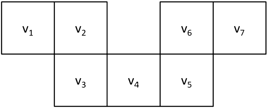For example, an agent with starting location in $v_{1}$ and goal location in $v_{7}$ in Fig. 3 has an abstract plan of seven locations. However, the physical agent has to perform four additional turning actions that the classical MAPF solvers do not take into consideration.

Fig. 3.

Example of graph where an agent has to perform turning actions.

As the abstract steps may have duration different from the physical steps, the abstract plans, which are perfectly synchronized, may desynchronize when being executed, which may further lead to collisions. This is even more probable in dense and optimal plans, where agents often move close to each other.

The intuition says that such desynchronization will indeed happen. In the paper, we will empirically verify this hypothesis and we will explore several abstract models for MAPF and output transformations to robot actions. These models not only try to keep the agents synchronous during the execution of the plan but also to avoid collisions caused by some small unforeseen flaw in the execution. We then compare and evaluate these models on an example grid using real robots. Note that the real robots only blindly follow the computed plan and cannot intervene if, for example, an obstacle is detected.

4. Models

In this section, we describe several variants of abstract MAPF models and possible transformations of abstract plans to executable sequences of physical actions. Let $t_{t}$ be the time needed by the robot to turn by 90 degrees to either side and $t_{f}$ be the time to move forward to the neighboring vertex in the grid. Both $t_{t}$ and $t_{f}$ are nonzero. The time spend while the agent is performing the wait operation $t_{w}$ will depend on each model.

4.1. Classic model

The first and most straightforward model is a direct translation of the abstract plan to the action sequence. We shall call this a classic model. At the end of each timestep, an agent is facing in a direction. Based on the next location, the agent picks one of the five actions described above and performs it. This means that all move actions consist of possible turning and then going forward. There are no independent turning moves.

The waiting time $t_{w}$ can be set arbitrarily, but in this case, we choose it to be $t_{f} + 1 / 2 * t_{t}$ reasoning that the two most common actions are (2) and (3, 4) and taking the average duration of them.

Note that this abstract model is the same as the typical definition of MAPF, and the solution (sequence of vertices for each agent) is translated into physical actions. Furthermore, we let the agents perform the actions without any delay (each moving action is performed as fast as possible).

4.2. Classic model with padding

One can easily see that the classic model can be prone to desynchronization, as turning adds time over agents that just move forward (different move actions have different durations depending on if turning is needed). Recall Fig. 3 and suppose there is another agent with the same number of steps, but all of the actions are moving forward. This agent will reach its goal $4 * t_{t}$ time units sooner than the agent from the example. This is not consistent with the abstract model, where all of the agents visit the vertices at the same time.

To fix this synchronization issue, we introduce a classic + wait model. The basic idea is that each abstract action takes the same time, which is realized by adding some wait time to “fast” actions as a padding. The longest action is (5), therefore each action now takes $2 * t_{t} + t_{f}$ including the waiting action $t_{w}$ . The consequence is that plan execution takes longer time, which may not be desirable.

The abstract model for classic and classic + wait models are the same, only the durations of the obtained physical actions differ.

4.3. Split actions model

One may desire to represent the executable actions directly in the abstract model. In particular, the need to turn can be represented by an abstract turning action. In the reduction-based solvers, this can be done by splitting each vertex $v_{i}$ from the original graph G into four new vertices $v_{i}^{up}, v_{i}^{right}, v_{i}^{down}, v_{i}^{left}$ indicating directions where the agent is facing to. The new edges now represent the turn actions, while the original edges correspond to move only actions, see Fig. 4. Note that when an agent leaves a vertex facing some direction, it will arrive to the neighboring vertex also facing that direction. This change to the input graph also requires a change in the MAPF solver (constraints), because the split vertices need to be treated as one to avoid collisions of type (ii). This means that at any time there can be at most one agent in those four vertices representing a given location. The abstract plan is then translated to an executable plan in a direct way as the agent is given a sequence of individual actions: wait, turn left/right, and move forward. In this case, the waiting time $t_{w}$ is set as the bigger time of the remaining actions: $t_{w} = max (t_{t}, t_{f})$ . We shall call this a split model.

Fig. 4.

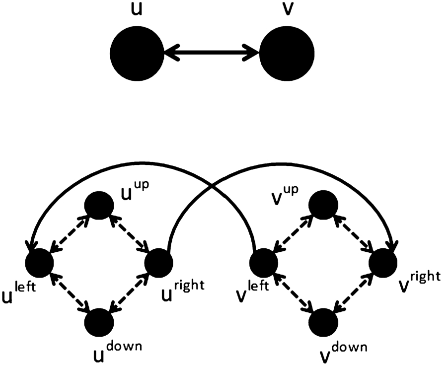
Example of how two horizontally connected vertices (top) are split into new vertices (bottom) describing possible agent’s orientations. The dotted edges correspond to turning actions.

4.4. Split model with padding

A synchronization issue is still present in the split model, if the times $t_{t}$ and $t_{f}$ are not the same. Recall that the solvers assume equal duration of all actions. One way to fix this is to use the trick with padding the “fast” actions with some extra waiting time.

This creates a split + wait model, where all physical actions take the same time. Specifically we set all actions to take $t_{w} = max (t_{t}, t_{f})$ . Note that this model may save some time over classic + wait since we add much less padding as a result of splitting the turn and move actions into two actions.

4.5. Weighted-edges model

Another way to solve the possible synchronization issue in the split model is to use a weighted MAPF [3]. Each edge in the graph is assigned an integer value that denotes its length. The weighted MAPF solver finds a plan that takes these lengths into account. Formally this can cause gaps in the plan of an agent as the agent may not be present in any vertex in the next step because the agent is still moving over an edge. This indeed does not break our definitions and the time is still discrete, only more finely divided. Also, note that it is needed to use a modified solver that can work with edges with non-unit length. Simply splitting the longer edges into several unit edges would allow the agents to turn or wait in the middle of the original edge, which is not allowed.

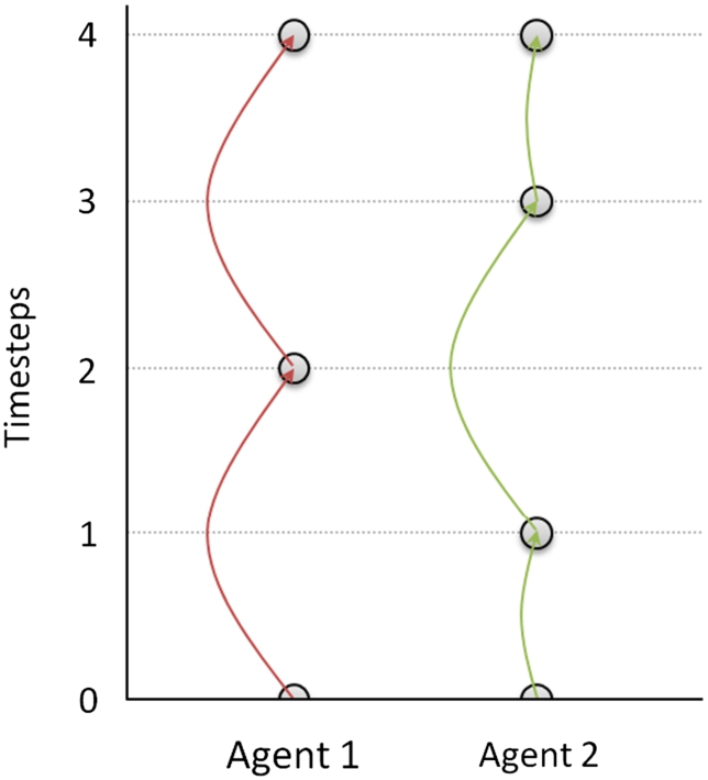
The lengths of turning edges are assigned a length of $t_{t}$ and the other edges are assigned a length of $t_{f}$ (or its scaled value to integers). The waiting time $t_{w}$ is set as the greatest common divisor of the remaining actions: $t_{w} = \gcd (t_{t}, t_{f})$ . We choose the greatest common divisor, so that an agent can wait exactly the length of any other action, while not granulating the actions too much. We shall call this a weighted-split model or w-split for short.

Fig. 5.

Example of a plan for two agents computed by w-split that do not arrive to some nodes at the same time. The red agent has planned a sequence of actions {move forward, move forward}, while the green agent has planned {turn right, move forward, wait}.

Table 1

Overview of all of the defined models

	No padding	Padding	No padding + robustness	Padding + robustness
Classic Model	classic	classic + wait	classic + robustness	classic + wait + robustness
Split Model	split	split + wait	split + robustness	split + wait + robustness
Weighted-Edges Model	w-split	–	w-split + robustness	–

Note that for the previous models (classic + wait, split + wait, and their robust variants), synchronization means that all agents leave and enter nodes in the original graph at the same time. This is not necessarily true for the w-split model. Let us assume, for example, that there are agents with $t_{t} = 1$ , $t_{f} = 2$ , and $t_{w} = 1$ . In this scenario, it is possible for two agents to have planed the following sequence of actions: {move forward, move forward} and {turn right, move forward, wait}. This scenario is shown in Fig. 5. Each plan has a duration of 4. While the first agent arrives to some nodes at times 2 and 4, the other arrives to a node at time 3 (at the time, the first agent is traversing some edge). This means that w-split is not synchronized in the sense that agents are arriving to nodes at the same time, but it is synchronized in the sense that the actions that are planned to happen at the same time are indeed happening at the same time.

4.6. Weighted-edges model with padding

While it was possible and useful in the two previous models to pad actions with waiting time so that they take the same time, it is not meaningful to do so with the w-split model. In this case there are still actions that take a different amount of time, however, these different times are incorporated in the theoretical model itself. For this reason, there is no need to create a new model with padding actions for w-split model.

4.7. Robustness

Some of the previously described models and translation to physical actions (theoretically) guarantee a perfect synchronization of the physical agents when performing the plan. However, as the agents are real robots moving in the imperfect real world, there still might be some desynchronization introduced during the execution. This desynchronization is not caused by the plan itself, but rather by some attributes of the environment. This may include imprecise speed of one of the robots, a wheel slipping, a roughness of the terrain, desynchronized start, and many more.

To minimize these effects, we may require the abstract plan to keep some space between the moving agents. We will use the notation from k-robust MAPF [1]. The k-robust plan is a valid MAPF plan that in addition requires for each vertex of the graph to be unoccupied for at least k time steps before another agent can enter it. Note that this is a change to the abstract model itself and needs to be performed by the solver, and it is not added during the translation of the abstract plan to the real actions. This enhancement can be added to all of the previously described models and can be combined with the padding translation to real actions. All that is left to do is to choose a proper k for each model.

For the classic type models, we choose k to be 1. We presume that this is a good balance between keeping the agents from colliding with each other while not prolonging the plan too much. For the split type models, however, it is not enough to use 1-robustness, as the plan is split into more time steps. Instead, we use $max (t_{t}, t_{f})$ -robustness.

4.8. Overview of models

In this section, we defined several models that can be seen in Table 1 for a quick overview. We defined three different approaches how to encode the MAPF problem (Classic, Split, Weighted-Edges) with a possible enhancement to the desired plan (Robustness). This creates six abstract models. The abstract models can then be translated to the real actions performed by the physical agents (these actions depend on the model). The translation can then be done by one of two ways – performing the action as fast as possible one after another with no padding, and adding padding to actions that take a shorter amount of time, so all actions take the same time. Note that for the w-split model this padding is equivalent with no padding, therefore we omit these two models. Together we defined ten models that can be experimentally tested.

5. Experiments

The proposed models for MAPF were empirically evaluated on real robots and in this chapter we will present the obtained results. We shall first give some details on robots, that we used, on the problem instances, and on a system, that was used to create these instances.

5.1. Ozobots

The robots used were Ozobot Evo from the company Evollve [10]. These are small robots (about 3 cm in diameter) shown in Fig. 6. We have chosen them because their built-in actions are close to actions needed in the MAPF problems so there is no need to do low-level robotic programming. The robots are programmable through a programming language Ozoblockly [7], which is primarily meant as a teaching tool for children. This can be seen in the simplicity of the drag-and-drop design of the language, see Fig. 7. The program is uploaded to the robot and then the robot executes it. Most importantly, the robots have sensors underneath that allow the robot to follow a line and to detect intersection. An intersection is defined as at least two lines crossing each other. The robots also have forward and backward facing proximity sensors allowing them to detect obstacles. We used them to synchronize the start of robots (see further), but we did not exploit sensors further during plan execution. In addition, the robots have LED diodes and speakers that act as the robots output. We use them to indicate some states of the robot such as a finished plan. The moving speed and turning speed can be adjusted up to a speed limit of the robot.

Fig. 6.

Ozobot Evo from Evollve used for the experiments. Picture is taken from [10].

Fig. 7.

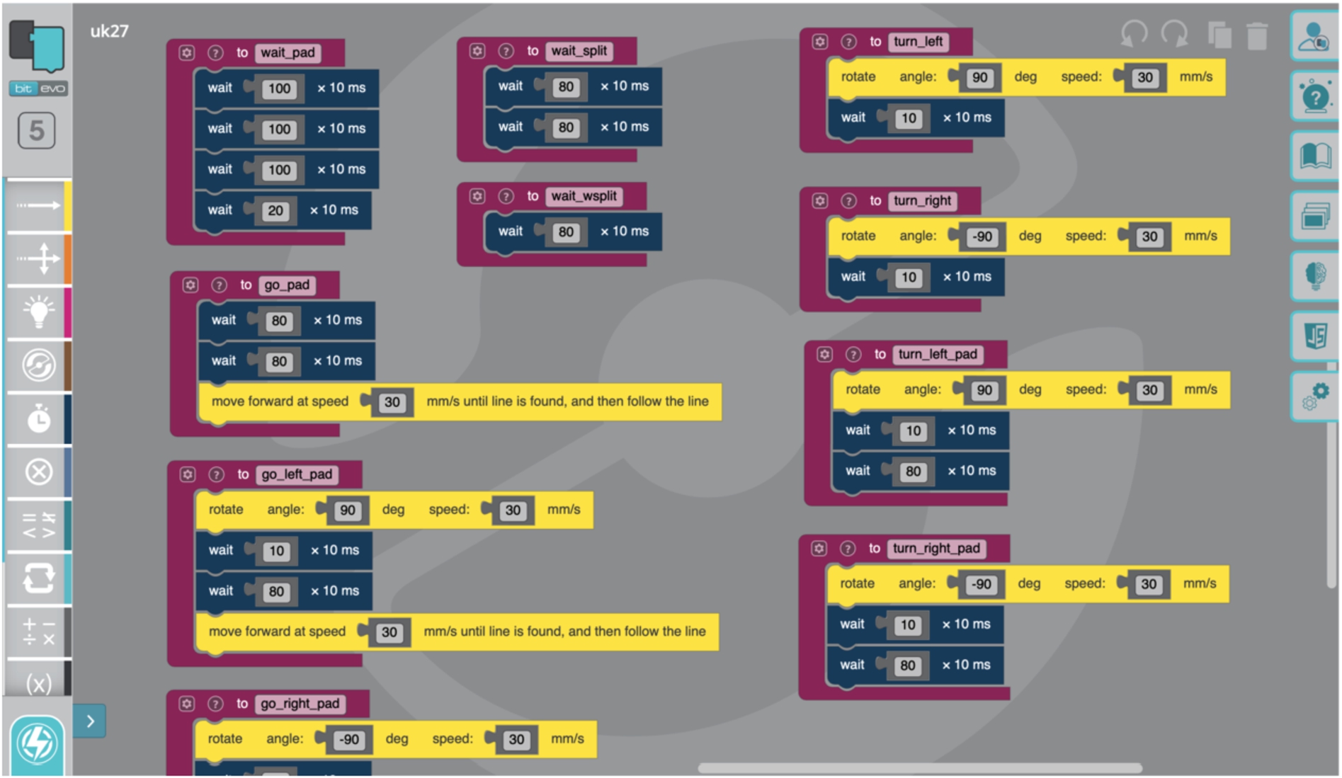
Example program coded in Ozoblockly language. The displayed procedures encode actions used by Ozobots for execution of MAPF plans.

There are some drawbacks in the simplicity of the robots. The main one is that there is currently no communication between multiple robots and therefore starting an instance of MAPF for all of the present robots at the same time is difficult. To solve this problem, we used the proximity sensors and forbid the agents to start performing the computed plan if an obstacle is present in front of them. An obstacle was placed in front of all of the agents and once all of them were ready to start executing the plan, all of the obstacles were removed. This ensured that the start time was identical and any desynchronization at the end of the plan was caused during the execution and not at the start.

5.2. MAPF scenario software

Fig. 8.

User interface of a system that lets user define and solve MAPF instances. The picture shows instance on a 4 by 4 grid map with obstacles and two agents (red and blue). The solution shown was computed by the model classic + wait.

To simplify the process of creating and solving MAPF instances, we designed a software MAPF Scenario that lets its user define grid maps, place agents and solve this instance with any of the models described above. We will describe some of the features of the system now. The user interface can be seen in Fig. 8.

First, a user needs to define a grid map over which the instance will be built or to load a previously created map. The user can define the dimensions of the grid, then obstacles can be introduced into the map by removing some of the vertices and edges of the graph. This map can be also printed on a paper, in which case, the user will be asked to define the length of the edges. A set of agents can be created on this map. For each agent, the user will be asked to specify its color, starting position, and goal position. The map and all agents specify the MAPF instance, which is displayed in the middle part of the user interface.

To solve the defined instance, the user can choose from ten different solvers, which correspond to the defined models in the previous section. Once a solution is found, the actions for each agent are displayed at the bottom part of the user interface. Note that each action has a defined duration it takes to perform it. This let us observe the total time of the plan on the timeline and the synchronization of the plan.

For even better visualization, it is possible to simulate the found plan on the displayed map. In such a case, circles representing the agents will appear and move in the map based on the actions shown in the bottom part.

Lastly, the user can choose to export the found plan to the Ozoblockly language that can be uploaded to the Ozobot robots. Running the plan on real robots rather than in simulation can show some further flaws in the plan caused by the dimensions of the robots and imperfections of the real world.

5.3. Problem instance

Using the MAPF system described above, several instances were crafted to test the defined models. These instances are shown in Figs 9–13.

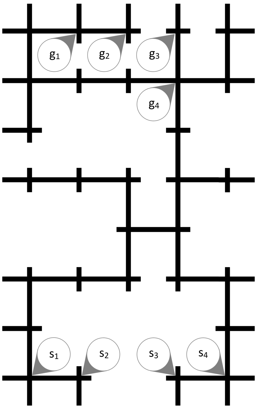
As opposed to the usual representation, where agents reside in the cells in between lines, here the agents follow the line and the vertex is represented as the crossing of two lines. These maps were printed on a paper in two scales. In the first scale, each edge is 5 cm long and the line is 5 mm thick as per Ozobots recommended specification. The edge length was chosen to allow two robots to safely stay in neighboring vertices and to observe even minor desynchronization due to turning. For the second scale, we doubled the length of the edges to 10 cm while keeping the thickness at 5 mm. This second scale was chosen to observe the behavior when robots are not as close to each other and thus allowing for bigger slack in the synchronization. We shall further refer to these sets of maps as smaller and larger maps.

Fig. 9.

Instance map for Ozobots called Bottleneck.

Fig. 10.

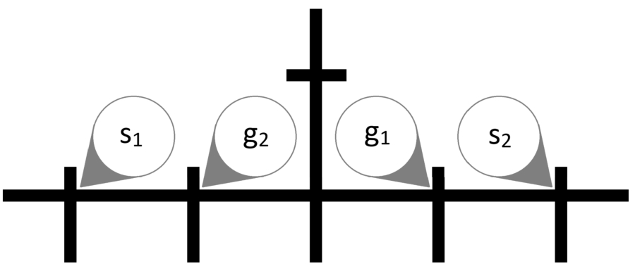
Instance map for Ozobots called Switch.

Fig. 11.

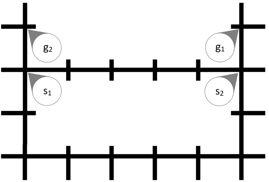
Instance map for Ozobots called Basket.

Fig. 12.

Instance map for Ozobots called Riddle.

In the Figs 9–13, the initial ( $s_{i}$ ) and goal locations ( $g_{i}$ ) are indicated. These circles were not printed, they are added as a notation for the reader. The robots are placed on the indicated initial location facing upwards (north). After reaching the goal location, it is not required to be facing any specific direction, only the presence at the specified intersection is required.

The speed of the robots was set in such a way that moving along 5 cm of a line takes 1600 ms (3200 ms for 10 cm lane) and turning takes 800 ms. This means that $t_{f} = 1600$ for smaller maps, $t_{f} = 3200$ for larger maps, and $t_{t} = 800$ . However, since all the numbers are divisible by 800, we can simplify the times for the MAPF solver to $t_{f} = 2$ for smaller maps, $t_{f} = 4$ for larger maps, and $t_{t} = 1$ . This then gives us all required times for the models as described in the previous section.

Each instance was designed to test some property of the theoretical models. Instance Bottleneck (Fig. 9) is the largest map, that forces four agents to pass through a narrow pass at roughly the same time, thus creating a bottleneck, where agents need to wait for others.

Instance Switch (Fig. 10) requires two agents to switch places. This map is very small and any desynchronization and close proximity can cause the agents to hit each other.

In instance Basket (Fig. 11) the two agents do not interact with each other, however, each agent has to travel a different distance. One will use the bottom path, while the other will use the top path.

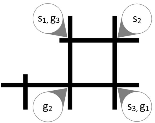
In instance Riddle (Fig. 12), three agents need to move along a cycle. This is again a very small map with big interaction between the agents.

Lastly, instance Spiral (Fig. 13) requires three agents to follow the spiral structure of the map. This requires the agents to turn many times, however, each agent turns a different number of times.

Fig. 13.

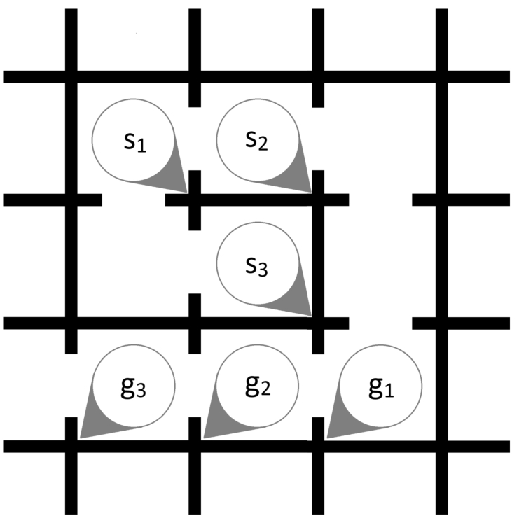
Instance map for Ozobots called Spiral.

5.4. Results

We generated plans using each MAPF model for all of the problem instances described above and then we executed the plans five times in total for each model. Several properties were measured with results shown in Tables 2–6. The tables show results for both smaller maps (left columns) and larger maps (right columns).

Computed makespan is the makespan of the plan returned by the MAPF solver. It is measured by the (weighted) number of abstract actions. Note that the split models have larger makespan than the rest because the split models use a finer resolution of actions, namely turning actions are included in the makespan calculation. This is even more noticeable with w-split and w-split + robustness, where the moving-forward action has a duration (weight) of two for smaller maps, respectively four for larger maps. Also note that for all models with the exception to w-split and w-split + robustness, the makespan for smaller and larger maps are identical. This is because there are no changes to the theoretical model if longer edges are used. Only the translation of the robot actions is different. On the other hand, w-split and w-split + robustness compute the solution using the length of the edges.

The number of failed runs is also shown. A model that had most often problems finishing the run is the classic model while the rest (with the exception of split and split + robustness in Bottleneck shown in Table 2) managed to finish all of the runs. A run fails if there is a collision that throws any of the robots off the track so the plan cannot be finished. One such collision can be seen in Fig. 14. The average number of collisions per run shows how many collisions that did not ruin the plan occurred. These collisions can range from small one, where the robots only touched each other (such as in Fig. 15) and did not affect the execution of the plan, to big collisions, where the agent was slightly delayed in its individual plan, but still managed to finish the plan. In the case that the execution fails, we present the number of collisions occurring before the major collision that stopped the plan.

Table 2
Measured performance of Ozobots on map Bottleneck (Figure 9) using each proposed model. The left columns are for 5 cm edges, the right columns are for 10 cm edges

Computed makespan Failed runs Number of collisions Total time [s] Max Δ time [s]

classic 17 17 5 0 3 0 NA 63.1 4 2.7

classic + wait 17 17 0 0 6 0 53.8 78.9 0 0

classic + robustness 19 19 0 0 0 0 40.4 68.7 1.2 1.1

classic + wait + robustness 19 19 0 0 0 0 59.9 88.2 0 0

split 27 27 0 5 4 1 37.6 NA 2 7.1

split + wait 27 27 0 0 3 0 44.2 85.2 0 0

split + robustness 28 28 5 5 2 1 NA NA 4.4 14.3

split + wait + robustness 28 28 0 0 0 0 46.1 88.2 0 0

w-split 44 80 0 0 1 0 37 65 0 0

w-split + robustness 44 80 0 0 0 0 37 65 0 0

	Computed makespan	Failed runs	Number of collisions	Total time [s]	Max Δ time [s]
classic	17	17	5	0	3	0	NA	63.1	4	2.7
classic + wait	17	17	0	0	6	0	53.8	78.9	0	0
classic + robustness	19	19	0	0	0	0	40.4	68.7	1.2	1.1
classic + wait + robustness	19	19	0	0	0	0	59.9	88.2	0	0
split	27	27	0	5	4	1	37.6	NA	2	7.1
split + wait	27	27	0	0	3	0	44.2	85.2	0	0
split + robustness	28	28	5	5	2	1	NA	NA	4.4	14.3
split + wait + robustness	28	28	0	0	0	0	46.1	88.2	0	0
w-split	44	80	0	0	1	0	37	65	0	0
w-split + robustness	44	80	0	0	0	0	37	65	0	0

Table 3

Measured performance of Ozobots on map Switch (Figure 10) using each proposed model. The left columns are for 5 cm edges, the right columns are for 10 cm edges

	Computed makespan		Failed runs		Number of collisions		Total time [s]		Max Δ time [s]
classic	6	6	1	0	1	0	14.3	22	2.6	2.3
classic + wait	6	6	0	0	1	0	18.2	26	0	0
classic + robustness	8	8	0	0	0	0	18.1	29.1	2.5	2.2
classic + wait + robustness	8	8	0	0	0	0	24.5	36.5	0	0
split	11	11	0	0	1	1	15	22	0.8	0.3
split + wait	11	11	0	0	0	0	18.1	34	0	0
split + robustness	11	11	0	0	0	0	14.3	22	0	0
split + wait + robustness	11	11	0	0	0	0	18.3	34	0	0
w-split	16	26	0	0	0	0	14.3	22	0	0
w-split + robustness	16	26	0	0	0	0	14.5	22	0	0

Table 4

Measured performance of Ozobots on map Basket (Figure 11) using each proposed model. The left columns are for 5 cm edges, the right columns are for 10 cm edges

	Computed makespan		Failed runs		Number of collisions		Total time [s]		Max Δ time [s]
classic	11	11	0	0	0	0	23.9	39.5	2.5	2.3
classic + wait	11	11	0	0	0	0	34.1	50	0	0
classic + robustness	11	11	0	0	0	0	21.3	37.1	0	0
classic + wait + robustness	11	11	0	0	0	0	34.1	50	0	0
split	15	15	0	0	0	0	22.4	39.4	1	2.2
split + wait	15	15	0	0	0	0	24.6	46.7	0	0
split + robustness	15	15	0	0	0	0	21.2	37.1	0	0
split + wait + robustness	15	15	0	0	0	0	24.6	46.7	0	0
w-split	25	45	0	0	0	0	21.4	37.1	0	0
w-split + robustness	25	45	0	0	0	0	21.4	37.1	0	0

Table 5

Measured performance of Ozobots on map Riddle (Figure 12) using each proposed model. The left columns are for 5 cm edges, the right columns are for 10 cm edges

	Computed makespan		Failed runs		Number of collisions		Total time [s]		Max Δ time [s]
classic	3	3	5	0	1	0	NA	11	1.7	1.9
classic + wait	3	3	0	0	2	0	8.6	11.5	0	0
classic + robustness	7	7	0	0	0	0	15.7	25.1	0.9	0.8
classic + wait + robustness	7	7	0	0	0	0	21.3	30.6	0	0
split	6	6	0	0	0	0	8.5	13.1	0.9	2.2
split + wait	6	6	0	0	2	0	10	18	0	0
split + robustness	8	8	0	0	0	0	11.2	17.1	1	2.2
split + wait + robustness	8	8	0	0	0	0	13.4	24.3	0	0
w-split	8	12	0	0	2	0	7.8	10.9	0	0
w-split + robustness	9	13	0	0	0	0	8.6	11.6	0	0

Table 6

Measured performance of Ozobots on map Spiral (Figure 13) using each proposed model. The left columns are for 5 cm edges, the right columns are for 10 cm edges

	Computed makespan		Failed runs		Number of collisions		Total time [s]		Max Δ time [s]
classic	14	14	5	0	1	0	NA	49.2	1.6	1.6
classic + wait	14	14	0	0	6	0	43.8	64.3	0	0
classic + robustness	16	16	0	0	0	0	32.7	56.3	1.7	1.5
classic + wait + robustness	16	16	0	0	0	0	50.1	74	0	0
split	22	22	0	0	0	0	30.3	52.3	1.3	2.3
split + wait	22	22	0	0	6	0	36.1	69.1	0	0
split + robustness	23	23	0	0	0	0	31.2	53.1	1.2	2.2
split + wait + robustness	23	23	0	0	0	0	37.5	72.2	0	0
w-split	36	66	0	0	0	0	30.2	54	0	0
w-split + robustness	36	66	0	0	0	0	30.2	54.1	0	0

Since we are using the makespan objective function, all of the plans can have their length equal to the longest plan without worsening the objective function. Even if the agents reached their destination sooner, their plan was prolonged by waiting actions to match the length of the longest plan. To visually observe this, we used the LEDs on the robots. The LEDs were turned on during the whole plan (including wait actions) and turned off once the plan was finished. This helped us to measure the overall time of the plan execution as the time from start to the last robot turning LEDs off. For the models that did not finish any of the five runs, there is no total time to show.

Table 7

Summary performance of Ozobots using each proposed model (quality indexes, larger value is better). The left columns are for 5 cm edges, the right columns are for 10 cm edges

	Computed makespan		Failed runs		Number of collisions		Total time [s]		Max Δ time [s]
classic	5.00	5.00	2.00	5.00	2.75	5.00	1.90	4.93	1.52	1.61
classic + wait	5.00	5.00	5.00	5.00	2.12	5.00	3.69	4.10	5.00	5.00
classic + robustness	3.95	3.95	5.00	5.00	5.00	5.00	4.12	3.98	2.64	2.74
classic + wait + robustness	3.95	3.95	5.00	5.00	5.00	5.00	2.79	3.08	5.00	5.00
split	3.04	3.04	5.00	4.17	3.70	4.00	4.80	3.72	2.35	1.82
split + wait	3.04	3.04	5.00	5.00	2.73	5.00	4.11	3.50	5.00	5.00
split + robustness	2.87	2.87	4.17	4.17	4.33	4.50	3.67	3.57	3.14	2.69
split + wait + robustness	2.87	2.87	5.00	5.00	5.00	5.00	3.83	3.29	5.00	5.00
w-split	1.97	1.15	5.00	5.00	3.83	5.00	4.99	4.88	5.00	5.00
w-split + robustness	1.92	1.13	5.00	5.00	5.00	5.00	4.88	4.82	5.00	5.00

Each individual agent was let to execute the plan without interference with other agents to measure the difference between the fastest and slowest agent as Max Δ time. If the agents are perfectly synchronized then this Δ should be zero. All of the times are rounded to one-tenths of a second because the measurements were conducted by hand.

From the number of collisions, the total times, and the Max Δ times, we can conclude some properties of the models. Indeed, models that have added + wait and w-split models keep the agents synchronous, while the other models do not (there is a gap between finishing the plans by different agents). From all models, the classic + wait + robustness model is the slowest one to perform the plan. This is expected as this model uses the longest durations of actions and furthermore, the robustness may add some extra steps to perform. We can see that by just splitting the actions in split models, we save some time even when we use the padding in models split + wait and split + wait + robustness.

Further, we can see that even if the agents are synchronous, some collisions may appear, since the agents have a nonzero diameter and if they are moving close to each other. This issue is solved by making a k-robust plan, however, if the agents are not synchronous, the agents can still collide.

Fig. 14.

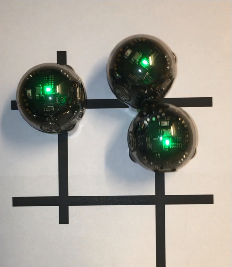
Example of collision that caused the plan to fail on instance Riddle solved by the model Classic. After the collision, the middle robot was unable to follow the line anymore.

Fig. 15.

Example of collision that did not cause the plan to fail on instance Riddle solved by the model Classic + wait.

Also note that on the larger maps, where the edges are longer and thus the agents are not moving close to each other, there are fewer collisions. This type of maps makes the robustness less useful, since even the non-robust plans do not usually collide. On the other hand, adding the padding in + wait models is counterproductive, because it prolongs the plans too much.

Desynchronization is still an issue even in the larger maps, even though it is not as much visible on any map with the exception of Bottleneck shown in Table 2. On the other maps, the plans are too short for the desynchronization to cause any collision, however, with longer plan we can see that the difference in individual plan lengths is large for split and split + robustness models.

Recall that adding + wait is just a change in translation of the plan to the actions, while adding + robustness requires to find a different plan. This can create a phenomenon seen in the results for instance Basket shown in Table 4. Here the plans for classic and split have the same makespan as classic + robustness and split + robustness respectively, while the Max Δ times are different. This is caused by the solver finding a different plan with the same length for each model. By a chance, the robustness models found a plan that was synchronous (each agent performed the same amount of turning and moving actions), while the classic and split models found a plan where the agents performed different actions.

To compare various models across different maps, we use a quality index (a similar index is used, for example, in International Planning Competitions). This index equals one for the best value of a given parameter and progressively decreases to zero for worse values. Formally, let $best$ be the minimal value of a given parameter across all models and a given map (we assume that the minimal value is the best value, which is the case of all evaluation parameters that we measured). Let $value$ be the value of the parameter for a given model and a given map. Then the quality index for that model and parameter equals $\frac{best}{value}$ . For parameters, where the minimal value can be zero (for example, the number of collisions), we used a modified version of the quality index $\frac{best + 1}{value + 1}$ . For non-finished runs we used a big number 6000 for the total time. Quality indexes are then summed across all the maps. The larger the sum is, the better the model is in that parameter. Table 7 shows the accumulated indexes for all five maps.

In general, we can see that simply translating the sequence of nodes to actions of robots is not enough to create a good executable plan. This can be solved by padding all of the movements with some waiting time so that the agents remain synchronous. However, this costs extra time during the execution. Splitting the actions to turning actions and moving actions provides us with finer granularity and thus a faster plan. This plan is still not synchronous, so padding is required to ensure the agents stay synchronous. The overall best solution is to take the action lengths into account while creating the plan. This allows the agents to stay synchronous without any extra waiting time, thus having the fastest execution time. Adding robustness furthermore betters the plan if the agents are moving close to each other. Table 7 confirms that robust plans are without collisions, but their execution takes more time.

6. Conclusion

In this paper, we studied the behavior of MAPF plans when executed on real robots. We defined several models that either take the classical plan and translate it into a sequence of robot actions or create a plan that already consists of the robot actions. This mainly included the need for turning of the robot. We discussed ways to keep the agents synchronized during the execution of the plan. This leads to either force the agents to wait for the other agents or to take the various lengths of the physical actions to account during the planning process.

The empirical evaluation confirmed the initial hypothesis that the classic model may have problems when executed on real robots. A bit surprising result was how many times it was not possible to complete the plan for the classic model. A straightforward translation to executable actions with identical duration resolved the issue of desynchronization but for the cost of a significant increase of the real makespan. The closer the model was to reality, i.e., assuming turning actions and weighted arcs to describe durations of actions, the better real makespan was obtained, which is somehow expected as the makespan of the abstract model, that is being optimized, is closer to the actual makespan. When we prolonged the edges to 10 cm, so the agents were more distant, then the classic model achieved surprisingly good results in terms of real makespan. However, this model still has the worst desynchronization, so when the plans become longer, one may expect an increased number of collisions there. Robustness generally helps to decrease the number of collisions, but one can observe that robustness itself does not prevent desynchronization.

The results provide some guidelines which model to select based on the environment. If the duration of turning is a significant portion of the duration of moving then the classic model is not applicable. The split model is particularly useful if these durations are close to each other, but the split model can be actually worse than the classic model if turning time is much smaller than moving time. The models with weighted arcs describing actual durations of actions provide the best actual makespan during executions, as expected, but the classic model is comparable with them if turning time is much smaller than moving time. In some sense, it justifies that the classic model is a viable abstract model. Still, one must be careful about synchronization issues for the classic model.

In the paper, we applied the MAPF plans on real robots, but we still used some assumptions such as that the robot moves with a constant speed. Exploring other ways of translating the abstract model to an executable model, for example, assuming kinematic constraints such as acceleration and deceleration, might be an interesting next step to improve further the quality of executable plans. Finally, the executed plans were static in the sense that robots just blindly executed them. By using information from sensors, the robot may prevent collisions by accommodating the plan to the current situation. For example, the robot may slow down (or even stop) to prevent collision with an unexpected obstacle and then the robot may speed up to catch up with the plan. For such dynamic execution of plans, it would be useful to have some flexibility in the plan that the control procedure can exploit.

Footnotes

Acknowledgements

This research is supported by the Czech Science Foundation under the project 19-02183S, by SVV project number 260 453 and by the Charles University Grant Agency under the project 90119.

References

Atzmon,

Felner,

Stern,

Wagner,

Barták and

Zhou, k-robust multi-agent path finding, in: Proceedings of the Tenth International Symposium on Combinatorial Search, Edited by Alex Fukunaga and Akihiro Kishimoto, Pittsburgh, Pennsylvania, USA, 16–17 June 2017,

Fukunaga and

Kishimoto, eds, AAAI Press, 2017, pp. 157–158, https://aaai.org/ocs/index.php/SOCS/SOCS17/paper/view/15797 .

Barták,

Švancara,

Škopková and

Nohejl, Multi-agent path finding on real robots: First experience with Ozobots, in: Advances in Artificial Intelligence – IBERAMIA 2018 – 16th Ibero-American Conference on AI, Proceedings, Trujillo, Peru, November 13–16, 2018,

G.R.

Simari,

Fermé,

F.G.

Segura and

J.A.R.

Melquiades, eds, Lecture Notes in Computer Science, Vol. 11238, Springer, 2018, pp. 290–301. ISBN 978-3-030-03927-1. doi:10.1007/978-3-030-03928-8_24.

Barták,

S˘vancara and

Vlk, A scheduling-based approach to multi-agent path finding with weighted and capacitated arcs, in: Proceedings of AAMAS 2018, Stockholm, Sweden, July 11–13, 2018, 2018.

Barták,

N.-F.

Zhou,

Stern,

Boyarski and

Surynek, Modeling and solving the multi-agent pathfinding problem in picat, in: 29th IEEE International Conference on Tools with Artificial Intelligence (ICTAI), IEEE Computer Society, 2017, pp. 959–966. doi:10.1109/ICTAI.2017.00147.

Boyarski,

Felner,

Stern,

Sharon,

Betzalel,

Tolpin and

S.E.

Shimony, ICBS: the improved conflict-based search algorithm for multi-agent pathfinding, in: Proceedings of the Eighth Annual Symposium on Combinatorial Search, SOCS 2015, Ein Gedi, the Dead Sea, Israel, 11–13 June 2015,

Lelis and

Stern, eds, AAAI Press, 2015, pp. 223–225, http://www.aaai.org/ocs/index.php/SOCS/SOCS15/paper/view/10974 . ISBN 978-1-57735-732-2.

Erdem,

D.G.

Kisa,

Öztok and

Schüller, A general formal framework for pathfinding problems with multiple agents, in: Proceedings of the Twenty-Seventh AAAI Conference on Artificial Intelligence, Bellevue, Washington, USA, July 14–18, 2013,

desJardins and

M.L.

Littman, eds, AAAI Press, 2013, http://www.aaai.org/ocs/index.php/AAAI/AAAI13/paper/view/6293 . ISBN 978-1-57735-615-8.

Evollve, Inc., Ozobot & OzoBlockly, Welcome to OzoBlockly, 2015. https://ozoblockly.com/.

H.A.

Kautz and

Selman, Planning as satisfiability, in: ECAI, 1992, pp. 359–363.

Kornhauser,

G.L.

Miller and

P.G.

Spirakis, Coordinating pebble motion on graphs, the diameter of permutation groups, and applications, in: 25th Annual Symposium on Foundations of Computer Science, West Palm Beach, Florida, USA, 24–26 October 1984, IEEE Computer Society, 1984, pp. 241–250. ISBN 0-8186-0591-X. doi:10.1109/SFCS.1984.715921.

10.

Ozobot & Evollve, Inc., Ozobot | Robots to code, create, and connect with, 2018. https://ozobot.com/.

11.

Ratner and

M.K.

Warmuth, NxN puzzle and related relocation problem, J. Symb. Comput. 10(2) (1990), 111–138. doi:10.1016/S0747-7171(08)80001-6.

12.

M.R.K.

Ryan, Exploiting subgraph structure in multi-robot path planning, J. Artif. Intell. Res. 31 (2008), 497–542. doi:10.1613/jair.2408.

13.

Sharon,

Stern,

Felner and

N.R.

Sturtevant, Conflict-based search for optimal multi-agent pathfinding, Artif. Intell. 219 (2015), 40–66. doi:10.1016/j.artint.2014.11.006.

14.

Sharon,

Stern,

Goldenberg and

Felner, The increasing cost tree search for optimal multi-agent pathfinding, Artif. Intell. 195 (2013), 470–495. doi:10.1016/j.artint.2012.11.006.

15.

T.S.

Standley, Finding optimal solutions to cooperative pathfinding problems, in: Proceedings of the Twenty-Fourth AAAI Conference on Artificial Intelligence, AAAI 2010, Atlanta, Georgia, USA, July 11–15, 2010,

Fox and

Poole, eds, AAAI Press, 2010, http://www.aaai.org/ocs/index.php/AAAI/AAAI10/paper/view/1926 .

16.

T.S.

Standley and

R.E.

Korf, Complete algorithms for cooperative pathfinding problems, in: IJCAI 2011, Proceedings of the 22nd International Joint Conference on Artificial Intelligence, Barcelona, Catalonia, Spain, July 16–22, 2011,

Walsh, ed., IJCAI/AAAI, 2011, pp. 668–673. ISBN 978-1-57735-516-8. doi:10.5591/978-1-57735-516-8/IJCAI11-118.

17.

Surynek, An optimization variant of multi-robot path planning is intractable, in: Proceedings of the Twenty-Fourth AAAI Conference on Artificial Intelligence, AAAI 2010, Atlanta, Georgia, USA, July 11–15, 2010,

Fox and

Poole, eds, AAAI Press, 2010, http://www.aaai.org/ocs/index.php/AAAI/AAAI10/paper/view/1768 .

18.

Surynek, On propositional encodings of cooperative path-finding, in: IEEE 24th International Conference on Tools with Artificial Intelligence, ICTAI, 2012, Athens, Greece, November 7–9, 2012, IEEE Computer Society, 2012, pp. 524–531. ISBN 978-1-4799-0227-9. doi:10.1109/ICTAI.2012.77.

19.

Surynek, Compact representations of cooperative path-finding as SAT based on matchings in bipartite graphs, in: 26th IEEE International Conference on Tools with Artificial Intelligence, ICTAI 2014, Limassol, Cyprus, November 10–12, 2014, IEEE Computer Society, 2014, pp. 875–882. ISBN 978-1-4799-6572-4. doi:10.1109/ICTAI.2014.134.

20.

Yu and

S.M.

LaValle, Structure and intractability of optimal multi-robot path planning on graphs, in: Proceedings of the Twenty-Seventh AAAI Conference on Artificial Intelligence, Bellevue, Washington, USA, July 14–18, 2013,

desJardins and

M.L.

Littman, eds, AAAI Press, 2013, http://www.aaai.org/ocs/index.php/AAAI/AAAI13/paper/view/6111 . ISBN 978-1-57735-615-8.

21.

Yu and

S.M.

LaValle, Planning optimal paths for multiple robots on graphs, in: 2013 IEEE International Conference on Robotics and Automation, ICRA 2013, 2013, pp. 3612–3617. ISSN 1050-4729. doi:10.1109/ICRA.2013.6631084.