Enhancing profit from stock transactions using neural networks

Abstract

Financial time-series forecasting, and profit maximization is a challenging task, which has attracted the interest of several researchers and is immensely important for investors. In this paper, we present a deep learning system, which uses a variety of data for a subset of the stocks on the NASDAQ exchange to forecast the stock price. Our framework allows the use of a variational autoencoder (VAE) to remove noise and time-series data engineering to extract higher-level features. A Stacked LSTM Autoencoder is used to perform multi-step-ahead prediction of the stock closing price. This prediction is used by two profit-maximization strategies that include greedy approach and short selling. Besides, we use reinforcement learning as a third profit-enhancement strategy and compare these three strategies to offline strategies that use the actual future prices. Results show that the proposed methods outperform the state-of-the-art time-series forecasting approaches in terms of predictive accuracy and profitability.

Keywords

Financial time series prediction stock price LSTM autoencoder feature engineering reinforcement learning

1. Introduction

Forecasting stock prices and maximizing profit is one of the most challenging machine learning problems today. The predicted price of a stock allows investors to ensure that they buy and sell the shares of various companies at the most opportune times, and enables them to maximize their profits. The prediction of stock prices is an interesting research area for both researchers and investors. While several forecasting models have been proposed [6,11,13,16,27,32,36,43], the problem of building a prediction model to forecast stock prices accurately is still an open question, and is under research.

Fig. 1.

The proposed deep learning framework for financial time series forecasting.

We use historical data to build a deep learning-based framework for the prediction of future stock prices and to enhance profitability. A number of different factors can affect the variation of stock prices. These include political and economic events, annual reports of companies, industry trends, market sentiments, historical prices, pandemics, share issue, and share buybacks [19]. While, it may be possible to build separate systems that predict stock prices from each of these factors and achieve accurate stock price predictions by combining their results, it is challenging to build a system that considers such a vast number of factors. On the other hand, historical patterns of stock prices include the effect of past events, and are the basis for technical analysis [20] of stock prices, which is used by investors and investment companies to predict stock trends. At present, technical analysis is used independently for predicting stock trends and providing advice to investors, and thus, historical stock prices can provide information to perform relatively accurate stock price predictions. While time varying distribution of data, and noise are two major reasons, why the problem of stock price prediction from historical data is challenging [40], a time series forecasting model which achieves high accuracy will be beneficial for the investors.

Profit from stock transactions can be enhanced by using genetic algorithms [38], reinforcement learning [5,48] or algorithms that use stock price predictions [33] to provide advice on when to buy or sell stocks. The efficacy of such algorithms is highly dependent on the accuracy of the stock price predictions. In our case, accurate predictions enable us to effectively use simple, greedy algorithms to provide advice on stock transactions. For our reinforcement learning model, we use per minute current and past price deviations and the current value of the stock owned as the inputs for the reinforcement learning model. Designing a trading strategy for maximizing the profit from stock transactions is challenging since it is difficult to achieve highly accurate predictions or to train reinforcement learning to achieve the maximum possible profit that can be achieved if all future prices are known.

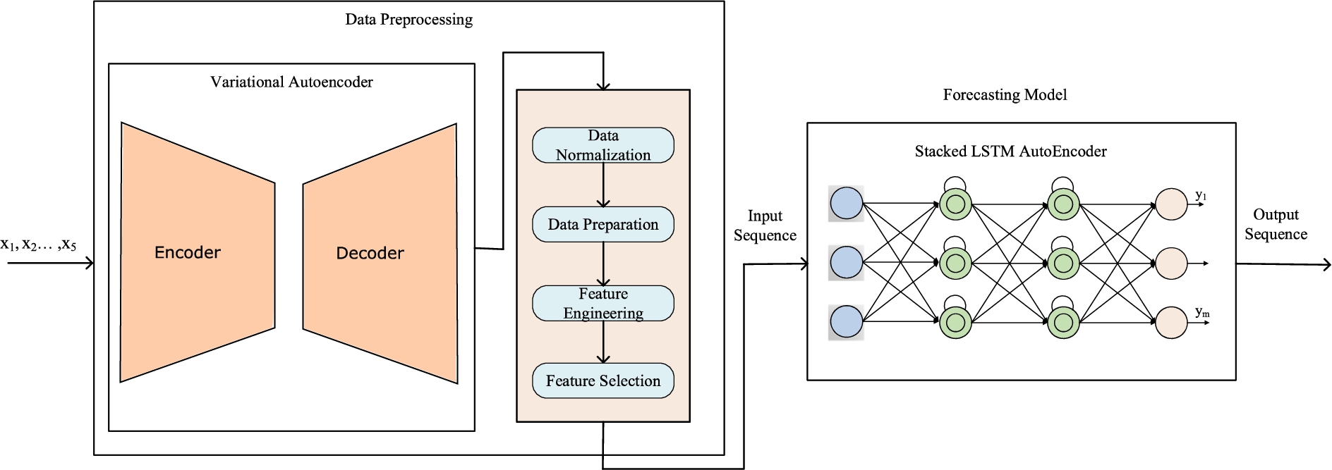
In this paper, considering the complexity of financial time series prediction and the applicability of deep learning in solving such problems [6,13,25], we propose a deep learning framework for stock price prediction and experimentally analyze the applicability and profitability of our framework. Figure 1 shows the proposed deep learning framework for financial time series forecasting. The framework uses an input sequence where each time lag of the input sequence has multivariate features: close, open, high and low prices, and volume. The output of the framework is an output sequence where each time lag of the output sequence corresponds to the stock closing price of the succeeding m time intervals. Therefore, our deep learning framework is designed for multi-step-ahead forecasting with multivariate input data. The output of the prediction framework is used as the input to two profit maximization strategies and the overall profit is analyzed. The strategies used include the use of short selling [3] as well as traditional stock transactions using greedy algorithms. Besides, we use a separate reinforcement learning [26] technique that does not use the predictions and only uses the current and past closing prices.

The proposed stock price prediction framework builds on our previous work in [1] and has two main components, data preprocessing and forecasting. Data preprocessing involves data normalization and data preparation, and may optionally include removal of noise, feature engineering, and feature selection. In data preprocessing, a variational auto-encoder (VAE) [23] is optionally applied on financial time series data with 5 features and is used to remove noise by generating a latent dimension from the original features. In addition, it can help to determine if an anomaly might happen. After applying the variational auto-encoder, the financial time series data has $5 + f^{'}$ features, where $f^{'}$ is the length of the latent features generated by the VAE. We then normalize the data by using Scikit-learn’s MinMaxScaler() [35] method in such a way that each feature of time series data has its own scaler. For data preparation, we use a sliding window which is moved from the beginning to the end of the data. For example, if we want to predict the stock closing price on $t + 1, t + 2, \dots, t + m$ times; $x_{t}, x_{t - 1}, \dots, x_{t - n}$ are used as the inputs to the model, and the output is $y_{t + 1}, y_{t + 2}, \dots, y_{t + m}$ where n is the length of the input sliding window and m is the number of steps ahead for prediction. After data preparation, we can optionally use feature engineering [10] and feature selection. Using feature engineering, we generate features which have basic and advanced statistical information regarding the financial time series data. In the next step, feature selection, those features which are more important are picked. The selected features are used as the inputs to our forecasting model. We use a stacked LSTM autoencoder as the forecasting model to predict the stock closing price for multiple steps in the future. We experiment with the different data pre-processing options and select the most suitable one. Our final stacked LSTM autoencoder uses the selected data pre-processing technique and is designed to predict the deviation of each of the next m minutes from the average closing price of the preceding n minutes.

Using the predicted stock prices, we design two algorithms to help the users to decide when to buy and sell a stock. The first algorithm uses a combination of short selling and traditional stock transactions to enhance profit in a manner similar to [6]. Based on the increase or decrease in price, this strategy decides to perform either short-selling or traditional transactions and the accuracy of the prediction determines actual profit or loss. The second algorithm does not employ short selling and uses a greedy approach to maximize the profit. Based on the predictions at time i, if the predicted closing price for any minute in the next m minutes is greater than the price at time $i + 1$ , we buy the stock at time $i + 1$ . Then we sell the stock at time $i + l$ , where predicted price at the lth minute of the output window is the maximum predicted price in the output window of m minutes. For the third approach, we use deep reinforcement learning to train an agent to select actions that maximize the reward. Specifically, we use Q-learning [46] to train a deep neural network to estimate the cumulative rewards for each possible action for a given state. For testing, the action that has the highest Q-value for a certain state is executed.

Besides, we design two offline strategies which give the optimal profits and are used for comparison only. The optimal profits can only be achieved if actual future stock prices are known. For the greedy offline strategy, the actual stock prices for the next m minutes are known and are used to make decisions about stock transactions. On the other hand, the optimal dynamic programming strategy knows the actual future prices for the entire span of the test set. This gives us the maximum possible profit that can be made by multiple stock transactions over the time period spanned by the test set. While it is not realistic for us to know the actual future stock prices, the profit that can be achieved in these cases is larger than the profit from any of our models or from Facebook’s Prophet.1

https://facebook.github.io/prophet/

This observation emphasizes the importance of accurate stock price predictions.

The novelty of our work lies in the following facts:

We use minutely data to perform multi-step-ahead predictions and make decisions. Since the change in price over milliseconds or seconds is too small, this reduces the profit that can be earned, especially if we consider the transaction fees [42]. On the other hand, the daily price movements are affected by random factors such as news, social behavior and other complex factors, and are thus, more difficult to predict [42].

We design algorithmic as well as reinforcement learning based approaches to decide when to buy or sell a stock in order to enhance profit.

Besides, we design two offline, optimal strategies to provide a measure of the profit that can be achieved if the actual future stock prices are known.

We compare the profits obtained from algorithms designed to use price predictions and reinforcement learning to optimal techniques that use the actual future prices. Thus, we provide a measure of the importance of accurate predictions and the degree of improvement in prediction accuracy that is necessary in order to match the profits from the offline algorithms.

Our prediction framework and the decision strategies can be extended to handle all the tickers in the NASDAQ stock exchange. We perform our experiments on 12 of the top 100 stocks on the NASDAQ exchange. However, since our framework trains a separate model for each stock ticker; if the necessary computational resources are available, it can easily be extended to handle all the tickers on the NASDAQ stock exchange.

The remainder of this paper is organized as follows. We discuss the related work in Section 2. In Section 3, a description of the inputs and the data resources is presented. Data preprocessing is discussed in Section 4 and the proposed deep learning framework for financial stock price prediction is discussed in detail in Section 5. The strategies for profit enhancement are discussed in Section 6. The experiments and results are presented in Section 7 and, finally, we conclude in Section 8.

2. Related work

The analysis of financial market movements and stock market forecasting has been widely studied in the last decade [4,24]. There are two approaches for the prediction and analysis of financial markets. The first approach is related to stock price movement forecasting, which is considered as a classification problem [13]. This approach investigates how to predict future market movements by mining information in textual format. Financial news and financial reports are considered as relevant sources of information for predicting the future market behavior [15,34,45,50]. The other method is to predict the value of the stock price, which is commonly regarded as a regression problem. The regression model used for stock price prediction deals with the problem as a time series prediction [9,22].

For the regression problem, two major classes of work, statistical models and machine learning approaches, have been used to forecast financial time series. Traditional statistical methods assume that financial time series are linear while many machine learning techniques capture non-linear relationships from data. Linear models such as ARIMA and ARMA have been widely used to predict financial time series [12,21]. Besides, various machine learning algorithms have been used in the area of stock prediction. Non-linear models such as Support Vector Regression, Neural Networks, and hybrid mechanisms have been utilized in stock forecasting and have achieved high predictive accuracy [6,11,16,27,32,36,43].

With the advent of deep learning, some researchers [6,13,33] have used deep neural networks to provide more accurate financial market predictions. However, this field remains relatively unexplored. There are related works that apply deep learning on financial data; for example, Ding et al. [13] use a deep convolutional neural network to predict the impact of events on stock price movements. Besides, deep belief networks have been utilized in financial market prediction [25]. Another work [6] proposes a method which uses stacked auto-encoders to predict the stock market. In [33], the authors develop a trading pipeline that uses the predictions from two LSTMs to develop a trading strategy for increasing profit. While one LSTM is used to predict the stock price trend, the second one is used to predict the stock trading price. In case of the second LSTM, the output prediction is corrected by using the error for the previous time step. In addition to the above prediction tools, some pre-processing approaches, such as Principal Component Analysis (PCA) [44], Discrete Fourier Transform [7], and Discrete Wavelet Transform [6], are used to remove noise and reduce the dimensions of raw data.

For the design of trading systems, several techniques have been proposed including ones that use genetic algorithms [38], and reinforcement learning [5,48]. In [38], a genetic algorithm is utilized to decide on the trading strategy. The price predictions used as the inputs to the trading strategy are obtained by using generalized moving averages. In [5,48], the authors use reinforcement learning to design a trading strategy. However, the approaches differ in terms of the information that is fed to the reinforcement learning model. While [5] uses stock trend predictions from sentiment analysis of news headlines as well as moving averages and current stock prices, [48] uses only the daily past and present stock prices without using any future predictions.

While some of the above works use statistical models [12,21] and machine learning techniques [11,16] that do not include deep learning, the use of deep learning [6,13,33] has led to a significant improvement in the accuracy of time series predictions. Our work involves the use of deep learning for stock price prediction and noise removal to ensure higher accuracy. With the advent of high frequency trading, there has been a shift towards autonomous trading involving high frequency predictions and actions performed by trained bots. The future of autonomous trading lies in the use of high-frequency data to perform a large number of hourly transactions. However, the existing works involve the prediction of daily stock prices only and are not suitable for high-frequency trading. In cases where the high-frequency data is used, it may be using data that has a frequency of around 1 second and utilizing a simple MLP model [14], or using Generative Adversarial Networks (GANs) to perform prediction of prices for a single step [49]. We use a dataset that allows us to utilize minutely data to perform multi-step ahead predictions and to provide minutely advice for stock transactions. We utilize an LSTM based autoencoder, which is more suitable than GANs for time-series prediction. To the best of our knowledge, algorithms and datasets that enable stock transactions based on minutely stock prices have not been explored previously. Our framework paves the way for research in the field of high-frequency stock price prediction, which, at present, has not been adequately explored.

3. Data description

We collect the features, which are depicted in Table 1, for 12 out of the top 100 stocks on the NASDAQ exchange and use this data as the input to our prediction framework. A listing of these stocks is found in Table 2. We collect data for 1-minute time intervals over a period of 5 months plus 1 week and use this historical data to build a model to predict the closing price of the stock.

Table 1
Iexfinance stock data sample features and their descriptions

Feature Description

marketOpen First price for the minute.

marketHigh Highest price for the minute.

marketLow Lowest price for the minute.

marketClose Last price for the minute.

marketvolume Total volume of trades for the minute.

Feature	Description
marketOpen	First price for the minute.
marketHigh	Highest price for the minute.
marketLow	Lowest price for the minute.
marketClose	Last price for the minute.
marketvolume	Total volume of trades for the minute.

Table 2

NASDAQ stock listing

Ticker	Company name
HAS	Hasbro, Inc
ADBE	Adobe
AAPL	Apple
FB	Facebook
EBAY	eBay
IDXX	IDEXX Laboratories, Inc.
GOOG	Google
COST	Costco Wholesale Corporation
AMZN	Amazon.com
FAST	Fastenal Company
INTC	Intel Corporation
CERN	Cerner Corporation

The source for our historical data is IEX Cloud,2

www.iexcloud.io

which provides data for 5 features for each time interval. The data is retrieved from IEX Cloud using a Python software development kit called iexfinance.3

www.github.com/addisonlynch/iexfinance

IEX Cloud provides several features for each stock polled. For our work, we focus on a stock’s open, high, low, and close prices as well as its volume for each time interval. Table 1 clarifies these features in more detail. The data collected for opening and closing prices are not constant for intra-day samples and instead reflect the relative price for the time interval on which the sample is collected. Since the data collected from IEX Cloud has some missing values, we use the backfilling method to deal with these missing values. Historical data from IEX Cloud is collected over a period of more than 5 months from March 01, 2019 until August 7, 2019.

4. Data preprocessing

Before feeding the data into a forecasting model, we preprocess the data. The data preprocessing component consists of multiple sections: removing noise using variational autoencoder, data normalization, data preparation, feature engineering, and selection. In Section 7, we evaluate whether the use of VAE and feature engineering provides benefits and incorporate the best performing combination of pre-processing methods in our final forecasting model.

4.1. Data normalization and preparation

4.1.1. Data normalization

We normalize the data using feature scaling to ensure that the multivariate input and multi-step prediction data that is fed to our model lies in the range $[0, 1]$ . The input to our prediction model uses 3-dimensional data of shape $[n_{s}, n_{t}, n_{f}]$ , where $n_{s}$ is the number of training samples, $n_{t}$ is the size of the input window (or lag) and $n_{f}$ is the number of features. We use Scikit-learn’s MinMaxScaler() tool for data normalization. Since this method requires the input to be 2-dimensional, our 3-dimensional input data with shape $[n_{s}, n_{t}, n_{f}]$ , which is required for LSTM modeling, is incompatible. Thus, we use two-dimensional input of shape $[n_{s}, n_{f}]$ , where the data is not formatted into separate input windows. Besides, it is desirable to have a distinct scaler for each of the features. To address the above issue, we take our 2-dimensional data of shape $[n_{s}, n_{f}]$ and restructure it into separate groups for each feature. Therefore, after restructuring, the number of groups is equal to $n_{f}$ and each group consists of 2-dimensional data of shape $[n_{s}, 1]$ . Once split, these groups are then normalized using Scikit-learn’s MinMaxScaler() method and merged into their original two-dimensional shape: $[n_{s}, n_{f}]$ . The benefit of this method is that we now have $n_{f}$ unique scaler objects which are mapped to each feature in our dataset. When our data is expanded to include the third dimension, $n_{t}$ , the expanded values will already be normalized and can be used to train the forecasting model. The $n_{f}$ scaler objects are then applied for inverse transformation after the model is built for forecasting and metric calculation.

4.1.2. Restructuring of data into input and output windows

Before feeding the normalized data to our forecasting model, we prepare the data by restructuring it into the overlapping sliding window format. Our original, normalized dataset has shape $[n_{s}, n_{f}]$ . For our predictions, we use n lag steps and m timesteps for each sample in our dataset to build a third timestep dimension for our data, where n is the length of the sliding window or input sequence, and m is the number of steps ahead for prediction. From the current sample, a window of width $n + m$ is constructed. For example, if we want to predict the stock closing price on times: $t + 1, t + 2, \dots, t + m$ ; the input of the model will be $x_{t}, x_{t - 1}, \dots, x_{t - n}$ , and the model output will be $y_{t + 1}, y_{t + 2}, \dots, y_{t + m}$ . By applying this method to all original samples, a restructured dataset is formed. This restructured dataset has shape $[n_{s}, n_{t}, n_{f}]$ . From this data, the defined window is used to make predictions from all of a stock’s features for the closing price $1, 2, \dots, m$ steps ahead.

As mentioned in the conclusion of [1], in this paper, the input and output window sizes are chosen empirically. We use input and output window sizes of 7 because, in most cases, increasing the input or output window sizes does not improve the accuracy of the results and only increases the computational overhead. This means that we look at the stock price at 7 steps before to predict the stock closing price for 7 steps-ahead.

4.1.3. Pre-processing to enable closing price deviation prediction

In [1], we use the above data preparation method and perform experiments on 5 tickers. However, when we attempted to use other tickers, especially INTC, we noticed a divergence in the predicted and actual values for those tickers that have a sharp decrease in price during the time interval that is used for testing. To overcome that issue, for each sample of shape $[n_{t}, n_{f}]$ , we modify the y values by subtracting the average of the preceding n closing prices. Thus, instead of trying to predict the closing price for the following m minutes, the prediction model tries to predict the deviation of the closing price at each of the next m minutes from the average closing price of the last n minutes. The average value is added back to the predicted deviations to get the predicted closing price for each of the following m minutes. We refer to this modification, which changes the task of the forecasting model as the deviation prediction technique.

4.2. Feature engineering and variational autoencoder

Here, we discuss the use of VAE and feature engineering. Our model is designed such that it may use one, both, or neither of these two techniques. In Section 7, we empirically choose one of the four possible combinations of these two techniques for our final model.

4.2.1. Variational autoencoder

In order to remove noise, we attempt to utilize a long short-term memory-based variational auto-encoder (LSTM-VAE) which consists of an encoder and a decoder. The encoder maps observations at each time step into a latent space. Then, the decoder estimates the expected distribution of the inputs from the latent space representation. The latent space has Gaussian distribution with $μ = 0$ and $σ = 1$ . In general, in VAE structure, the encoder first projects an instance into a mean value and standard deviation of a latent variable and then does sampling from the latent variable’s distribution. In the second step, the decoder decodes the samples into a mean value and standard deviation of the output variable and then generates samples from the output variable’s distribution. In addition to the original 5 features: close, open, low, high, and volume, we use the latent features generated from the original features. The latent features are expected to help in removing noise, as it can help determine if an anomaly might happen. So after applying the variational auto-encoder, the financial time series data has $5 + f^{'}$ features, where $f^{'} = 5$ , which is the length of the latent features generated by the VAE. In [1], we use the VAE as part of the data pre-processing for our prediction model. In Section 7, we show that the use of the VAE does not improve the results when compared to data pre-processing that uses feature engineering but no VAE.

Fig. 2.

LSTM autoencoder sequence to sequence model.

4.2.2. Feature engineering and feature selection

For feature engineering, the normalized and prepared data are given to a module and is used to extract a new set of features. Our data is time series data, so we need to use time series feature extraction techniques to map the data into a high dimensional feature space. We use tsfresh [10], which is an excellent tool for extracting features from time series data. tsfresh is capable of handling multivariate time series data sets and is implemented in Python.4

⁴
https://tsfresh.readthedocs.io/en/latest/text/introduction.html

The features extracted by tsfresh include basic and advanced characteristics of the time series. tsfresh computes the following features from each variable of the stock time series data (naming reflects the tsfresh standard): maximum, minimum, mean, median, standard_deviation, abs_energy, kurtosis, skewness, mean_abs_change, and mean_change. In total, tsfresh extracts 750–850 features for each stock. Before we process the features, we impute them using tsfresh’s internal impute function.5

⁵

https://tsfresh.readthedocs.io/en/latest/_modules/tsfresh/utilities/dataframe_functions.html#impute

This is done to replace features output by tsfresh that are nulls.

Next, we rank the features according to their importance and then use this rank to perform feature selection. We try to use SelectKBest and RFECV, both of which are implemented in ScikitLearn, to rank all the features. SelectKbest ranks each feature through a scoring function and RFECV eliminates features at each iteration and is called recursive feature extraction with cross-validation [17]. Comparing SelectKBest and RFECV, we do not observe any significant differences in the accuracy of the predictive models. This shows that both of these feature selection approaches are almost equally effective. We use only the top 20 features produced by SelectKBest to reduce training and testing times. Besides, we observe that the use of more features does not significantly improve the accuracy.

Fig. 3.

The general network architecture used for building the learning model.

5. Forecasting model

5.1. Learning model

We use Long Short-Term Memory Networks (LSTMs) [18] for building our learning model. LSTMs are a special kind of Recurrent Neural Networks (RNNs) which solve the gradient vanishing and exploding problem that the standard version of RNNs suffer from. The LSTM structure is well-suited for time series prediction with different number of time lags. For our experiments, we use the Keras framework,6

⁶
https://keras.io/

which is a high-level neural network API written in Python.

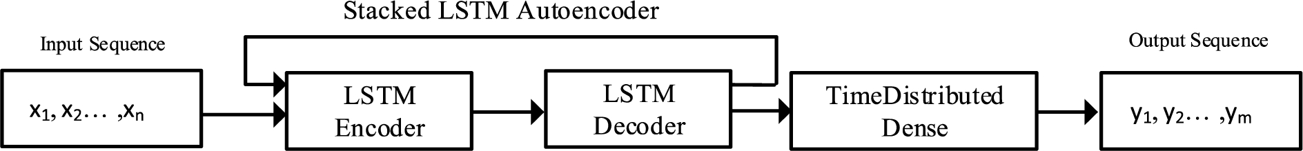
In our learning model, we use a stacked LSTM Autoencoder as the reference architecture for our neural network. An LSTM Autoencoder built using an Encoder-Decoder LSTM architecture can be utilized for sequence to sequence problems. A sequence to sequence (seq2seq) prediction model takes a sequence as input and predicts an output sequence. It is challenging to use such prediction models in cases where the length of the input and the output sequences are not fixed. However, LSTM Autoencoders have been effectively used for seq2seq prediction problems [39,47], where the encoder reads the input sequences and compresses it to a fixed-length internal representation, while the decoder interprets the internal representation and uses it to predict the output sequence. An LSTM Autoencoder is shown in Fig. 2. LSTM Autoencoders have been used to process video [37] (Image Captioning), text [31] (Machine Translation), audio (speech recognition) [29], and time series sequence data [28,30].

The general structure of LSTM Autoencoder architecture used in our work is presented in Fig. 3. We have an Encoder model that reads the input sequence and outputs an element vector that captures features from the input sequence. The decoder returns the entire output sequence. For example, if we have 10 cells in the last layer of the decoder, each of the 10 cells will generate outputs for each of the timesteps in the output sequence. In the output layer, we use the $TimeDistributed$ Keras wrapper around the final $Dense$ layer in order to ensure that the $Dense$ layer is applied independently to the output for each timestep. Our encoder consists of a LSTM layer of 200 neurons. The decoder consists of 2 layers of LSTMs and a dropout layer. Each of the 2 LSTM layers in the decoder consists of 200 neurons. The network, therefore, outputs a three-dimensional vector with the same structure as the input, with the dimensions $[n_{s}, n_{t}, n_{f}]$ . Since we predict the stock closing price, for 7 step-ahead, the output sequence shape will be $[1, 7, 1]$ .

Our learning model takes a sequence of stock prices and features of n lags and predicts the output as a sequence with length m. Each lag in the input sequence has multiple features such as opening price, closing price, low price, high price, and volume. Some other features may be added in the feature engineering step discussed in Section 4.2. Each element in the output sequence corresponds to the stock closing price at time step t, where $0 < t < m$ . Thus, we use our learning model as a stacked LSTM Autoencoder for multi-step forecasting with multivariate input data.

5.2. Hyperparameter optimization

Since neural networks like LSTM need to utilize hyperparameter optimization for selection of hyperparameters, we attempt to use the Hyperas7

⁷
http://maxpumperla.github.io/hyperas/

Python package. Hyperas is a wrapper around Hyperopt which enables fast prototyping of Keras models. For each of the 12 tickers, the hyperparameter optimization is performed separately. Due to the computational complexity of this task, we limit the maximum number of evaluations for each ticker to 100 and use only the first two months of our data for performing the optimization. The last one-third of that data (20 days) is used as the validation set and the remaining data (around 40 days) is used as the training set for hyperparameter optimization. The Hyperas Python package performs hyperparameter optimization by using different combinations of the values to train separate models and evaluating the models on a validation set. The algorithm aims to find the optimal combination of values by searching the search space and minimizing the loss on the validation set. Hyperas uses a Tree of Parzen estimators [8] to effectively search the search space and identify appropriate hyperparameters. The optimized hyperparameters are:

Number of epochs

Batch size

Learning rate

The dropout value for the dropout layer

Fig. 4.

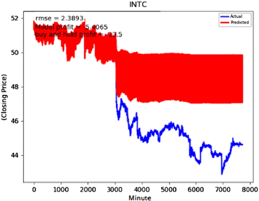
INTC predictions without hyperparameter optimization or the use of the deviation prediction technique.

Fig. 5.

INTC predictions using hyperparameter optimization without the deviation detection technique.

In models where we do not use the deviation prediction technique, we see significant improvement in the performance especially for tickers for which we do not get suitable performance with the default hyperparameters. An example of one such ticker is INTC. In Figs 4 and 5, we provide the results of INTC ticker before and after using hyperparameter optimization. In Table 3, we provide the root mean square error (RMSE) and the profit as described in [1] before and after hyperparameter optimization. Besides, we tabulate the results for the same quantities after using the deviation prediction technique but without hyperparameter optimization. The RMSE is reduced by using hyperparameter optimization without introducing the deviation prediction method. However, the RMSE shows a more significant decrease when we introduce the deviation prediction method even without performing hyperparameter optimization. In Fig. 6, we provide the plot for INTC after using the average subtraction technique.

Table 3

Comparison of INTC models with or without use of hyperparameter optimization and deviation prediction

Model	RMSE	Profit
No optimization, no avg subtraction	2.3893	−5.41
Optimization, no avg subtraction	1.0990	2.6603
No optimization, avg subtraction	0.0395	125.34

Fig. 6.

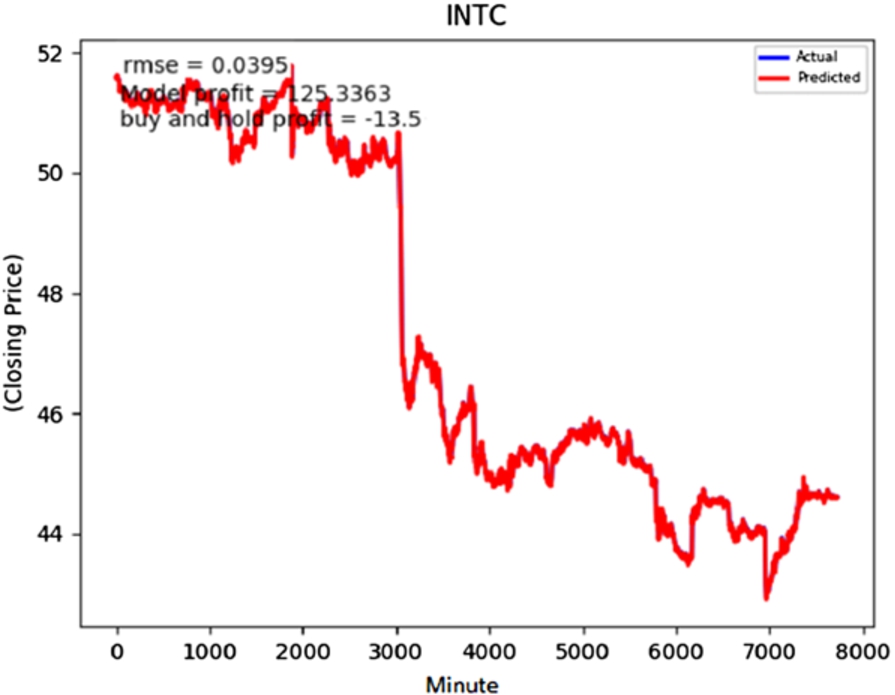
INTC predictions without hyperparameter optimization but using the deviation prediction technique.

Fig. 7.

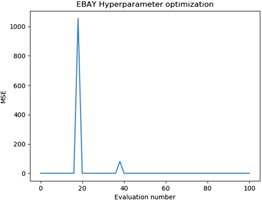
EBAY variation of MSE over hyperparameter optimization evaluations.

Since the stock data for almost all tickers includes a certain amount of randomness, retraining an architecture with the same hyperparameters on the same data can result in models that vary moderately from each other. This causes a challenge in case of hyperparameter optimization especially for the models that use the deviation detection technique because the error in those cases is small. Thus, it is difficult to separate the error due to the use of a model without optimized hyperparameters and error due to the randomness in the data. The effect of randomness can mask or have an equal impact as the improvement due to optimization making it hard for the algorithm that we use to search the hyperparameter space effectively. In Fig. 7, we plot the mean square error (MSE) for EBAY over different evaluations of the hyperparameter optimization algorithm for models that use the subtraction of averages technique. As we see from the figure, there is no significant improvement in accuracy over time. The actual MSE values corresponding to those that are near 0 are in the range of 0.00056 and 0.00037 on the validation set. However, each hyperparameter optimization can take up to 21 hours on a NVIDIA 2080Ti GPU and due to the difference in the distribution of data for each of the tickers the optimization needs to be performed individually for each ticker. Besides, the error is already low without using hyperparameter optimization if we use the deviation detection technique. Thus, we choose not to perform such computationally expensive operations that do not lead to a definite and significant improvement in performance.

6. Profit enhancement strategies

6.1. Strategy 1: Using short selling and traditional transactions (SS&T)

In [6], a profitability measure is introduced, which uses a buy-and-sell trading strategy. As shown in equation (1), the strategy states that investors should buy if the model predicts that the stock value is going to increase in the next time interval. In accordance with equation (2), if the model predicts a decrease in the stock price, the investors are recommended to sell. The variables ${\hat{y}}_{t + 1}$ and $y_{t}$ correspond to the predicted value for the next period and the actual value for the current time, respectively. Therefore, if the model predicts that the stock goes up, and the price does actually go up, the investors gain by an amount equal to the change in the price of the stock. However, if the price goes down, the investors suffer a loss which is equal to the decrease in price. The same logic is applied when the model predicts a decrease in the stock price. The buy-and-sell trading strategy is described in equation (3). $\begin{array}{l} (1) & B = {t ∣ {\hat{y}}_{t + 1} > y_{t}} \\ (2) & S = {t ∣ {\hat{y}}_{t + 1} < y_{t}} \\ (3) & \begin{matrix} \frac{R}{100} = & \sum_{t \in B} \frac{y_{t + 1} - y_{t} - 2 * T_{f}}{y_{t}} \\ + \sum_{t \in S} \frac{y_{t} - y_{t + 1} - 2 * T_{f}}{y_{t}} \end{matrix} \end{array}$

Here, R is the amount gained by using the strategy, while B and S indicate the minutes at which shares are bought for traditional selling or short sold, respectively. $T_{f}$ is the transaction fee for each transaction. Based on online applications such as Robinhood, the regulatory trading fees per share is $$ 0.000119$ .8

⁸
https://d2ue93q3u507c2.cloudfront.net/assets/robinhood/legal/RHF%20Retail%20Commissions%20and%20Fees%20Schedule.pdf

In case we predict an increase in the stock price at time

t + 1

, we buy the share at time t and sell it at time

t + 1

. If the predicted trend is correct, we make a profit, and the actual profit or loss is

y_{t + 1} - y_{t}

. In case we predict a decrease in the stock price at time

t + 1

, we use short selling to ensure profit. Here, selling short involves borrowing a stock, selling it when the price is higher at time t, buying it back when the price is lower at time

t + 1

and then returning it to the lender. If the prediction is correct in terms of the trend, this allows us to make a profit of

y_{t} - y_{t + 1}

6.2. Strategy 2: Greedy strategy (Greedy)

We introduce a greedy strategy that uses the predictions for the next 7 minutes. At a specific minute, say $i - 1$ , we generate the predicted prices for the next m minutes, $[i, i + 1, \dots, i + m - 1]$ . If the actual closing price at the ith minute is greater than each of the predicted closing prices for the next $m - 1$ minutes, then we do not perform any transactions for minute i. However, if there is any minute in the succeeding $m - 1$ minutes of the output window, where the predicted closing price is greater than the actual closing price at minute i, then we buy the stock at the ith minute. We find a minute $i + l$ in the output window such that $1 ⩽ l ⩽ m - 1$ and the predicted closing price at $i + l$ is the maximum for the output window. Since, at minute $i + l$ , the predicted closing price is expected to be maximum for the output window starting at time i, our strategy sells the stock at the selected minute $i + l$ . Thus, if there is an increase in price from minute i to minute $i + l$ , we make a profit. In case our predictions are incorrect and the price decreases from minute i to minute $i + l$ , we incur a loss. We repeat the same process for the output window starting from minute $i + l + 1$ in case we choose to make transactions during the current output window. Otherwise, we repeat the process for the output window starting at time $i + 1$ . We provide the pseudo-code in Algorithm 1, where we use the 2D array, L_predicted and the 1D array L_actual as inputs. Each element, L_predicted[i] of array L_predicted, has m elements where the first element in L_predicted[i] is the predicted price for minute i predicted using data for time $[i - n, \dots, i - 1]$ . L_actual[i] is the actual stock closing price at time i.

Algorithm 1:

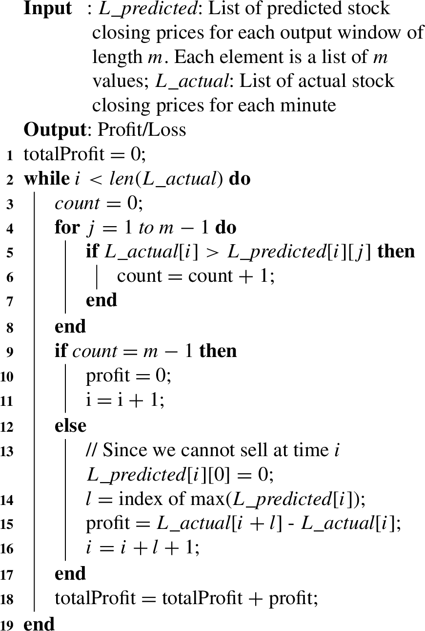
Strategy 2: Greedy strategy

6.3. Strategy 3: Reinforcement learning (RL)

We use Q-learning [46] to design our third profit enhancement strategy. In Q-learning, an agent attempts to maximize its rewards when it acts in a specific environment. In our case, the environment is the stock market for a specific ticker and the agent attempts to maximize its reward (profit) by buying and selling stocks in this environment. Specifically, we provide the information about the current state, $s_{j}$ to the agent, and the agent takes an action, $a_{i}$ , from a set of possible actions, A, to go to the next state, $s_{j + 1}$ while receiving a reward, r. It is the agent’s task to learn to select an action in A for state $s_{j}$ , so as to maximize total profit. For this purpose, the agent tries to learn a policy, π, that maps a state, $s_{j}$ to an action, $a_{i}$ , that results in maximum cumulative reward. In order to ensure adequate performance, it is important to consider the future as well as the current reward. Thus, a factor, γ, is introduced as a discount factor to discount the future reward as immediate rewards are given higher importance than future ones. A Q-value function is used to estimate the value of an action, $a_{i}$ , taken at state $s_{j}$ . It considers the cumulative reward function as: $r_{0} + \sum_{t > 0} γ^{t} r_{t}$ . For any state, $s_{j}$ , the action with the highest Q-value is selected and executed by the agent.

Computing the Q-value for all the states is computationally intractable due to the large number of possible future states as well as the necessity of computing the rewards for all these states and using the cumulative future reward for computing the Q-value of the current state. As a result, a deep neural network is trained to estimate the Q-value function and then the action with the highest predicted Q-value for state $s_{j}$ is taken during the testing phase. In our case, the training is performed as episodes where the agent performs buy and sell operations over the entire training set and, for each state, $s_{j}$ , the action, $a_{i}$ , reward r, and next state, $s_{j + 1}$ , are stored in a fixed length memory of size $M_{s}$ . After every $t_{s}$ steps, we select a minibatch of size $b_{s}$ from this memory, and train the network using Adam Optimizer. For a state, say $s_{j}$ in the minibatch, the training minimizes the mean square error (MSE) between the estimated Q-value for the state-action pair, $s_{j}$ , $a_{i}$ , and the Q-value computed by summing the actual reward, r, and the discounted maximum estimated Q-value of the next state. The MSE loss minimized is the summation of losses of all the state-action pairs in the minibatch. In order to ensure that new state-action pairs are explored by the agent during training, an exploration rate, ϵ, is used. An action is selected at random with probability, ϵ, at each step in each episode and otherwise we select the best action for that state. We use a higher value of ϵ at the beginning and then decay it slowly over a number of steps till it reaches a minimum value after which we do not decay ϵ further. During the testing phase, exploration is not used and the agent takes the action that has the highest Q-value for each state.

For our Q-Learning strategy, we design an environment where the agent is allowed to buy one stock for a specific ticker and sell it before it can buy another one. While we can use a situation where we give the agent a certain amount of cash and allow it to buy as many stocks as possible with this amount before it must sell in order to buy more stocks; we choose this environment to ensure compatibility with our other strategies. We use an approach similar to [2]. The state, action, and reward in our case are as follows:

State: The state consists of the last $n_{d}$ closing price deviations. Specifically, the value of deviation at time t is $closing_{price}_{t} - closing_{price}_{t - 1}$ . Besides, the state stores the deviation of current price of the stock from the price at which it was bought as well as the number of stocks owned at present.

Action: The possible actions are as follows:

Buy: Buy a stock of the company

Sell: Sell a stock of the company

Hold: Perform no action. The number of stocks owned does not change.

Reward: Profit/ Loss from current action. We get a profit or loss of $s - p$ when we sell a stock at s and had bought it for p.

We use 250 epochs and a learning rate of 0.001 to train our Q-learning network. We perform training separately for each ticker. Our network consists of 3 linear layers with the first 2 layers using ReLU activation function.

6.4. Offline strategies

For the purpose of comparison, we design two offline strategies, which use the actual future values to decide on the action that is to be taken. These strategies cannot be used in real-life because actual future stock prices are not known to us.

6.4.1. Offline greedy strategy (Greedy-O)

We design an optimal greedy strategy similar to the one described in Section 6.2. However, this offline strategy uses only actual data and does not use any predicted data. Thus, the decisions made are always correct because the actual future data for the next m minutes is known at the time of making the decisions. This is used for comparison to show the benefit of accurately knowing the future.

6.4.2. Offline dynamic programming (DP-O)

The offline dynamic programming strategy gives the maximum amount of profit that can be earned for a specific stock over a period of time. It uses actual (not predicted) future data for the entire future to make decisions. Dynamic programming is used to find the maximal profit if we are allowed to perform at most one transaction per minute. Using the actual future stock prices, we can compute the specific minutes at which to buy and sell a stock in order to maximize the profit. This is an optimal strategy and is used for comparison to show the maximum possible profit.

7. Experimental results

In order to validate the general forecasting performance of our proposed prediction models, we perform multiple experiments to evaluate the stock closing price prediction for different types of stocks with a variety of different patterns and behaviors. For the experiments, we use historical minutely data from IEX Cloud collected over a period of more than 5 months from March 01, 2019 until August 7, 2019. We choose 12 tickers out of the top 100 stocks on the NASDAQ exchange and evaluate our model. The chosen tickers are listed in Table 2. Besides, we evaluate the profits from our strategies and compare those to baseline and optimal strategies.

We use the first M minutes of training data for training and last L minutes for validation, where $L < M$ . This ensures that time dependence is maintained.

7.1. Data splits, baseline and forecasting models

We use almost the first 16 weeks of the data for training and then use the data for the remaining 7 weeks for testing. For the evaluation and experiments, we use historical minutely data for the 12 selected tickers.

We compare our models with: Prophet,9

⁹
https://facebook.github.io/prophet/

which is the Facebook time series package. The various prediction models that we compare are as follows:

Prophet: A time series forecasting method presented by Facebook’s data science team [41].

LSTM: Applying Long Short-Term Memory neural network on prepared data without feature engineering and without removing noise.

LSTM + VAE: Applying Long Short-Term Memory neural network on prepared data after removing noise.

LSTM + VAE + FE: Applying Long Short-Term Memory neural network on features extracted from prepared data after removing noise.

LSTM + FE: Applying Long Short-Term Memory neural network on features extracted from prepared data without removing noise.

LSTM + VAE + AVG: Applying Long Short-Term Memory neural network after removing noise from the input data but without using feature engineering. We use the model to predict the deviation in each minute from the average of the closing prices for the last 7 minutes.

The profit enhancement strategies compared and the baselines are:

Strategy 1: Short-selling and traditional transactions (SS&T): The strategy that uses short-selling and traditional transactions based on future predictions as discussed in Section 6.

Strategy 2: Greedy Strategy (Greedy): Uses the greedy method described in Section 6.2 and involves the use of traditional transactions only (no short selling).

Strategy 3: Reinforcement Learning (RL): Uses reinforcement learning model as described in Section 6.3.

Prophet: A time series forecasting method presented by Facebook’s data science team [41]. We use the SS&T technique to compute the profit using Prophet’s predictions.

Buy and hold (B&H): Buy at the beginning of the test data time and sell at the end.

Offline Greedy strategy (Greedy-O): As described in Section 6.4, this greedy strategy uses the actual future prices to make decisions.

Offline Dynamic Programming (DP-O): As described in Section 6.4, this strategy uses dynamic programming and actual future prices to compute the maximum possible profit.

7.1.1. Predictive performance

In this study, we use three metrics in order to measure the predictive accuracy: Root Mean Squared Error ( $RMSE$ ), Mean Absolute Percentage Error ( $MAPE$ ), and coefficient of determination ( $r^{2}$ ).10

¹⁰
https://www.statisticshowto.datasciencecentral.com/probability-and-statistics/coefficient-of-determination-r-squared/

\hat{y}

is the predicted value, and y is the value of the actual observation, then

RMSE

MAPE

, and

r^{2}

are defined as follows:

\begin{array}{l} (4) & RMSE = \sqrt{\frac{1}{n} \sum_{i = 1}^{n} {({\hat{y}}_{i} - y_{i})}^{2}} \\ (5) & MAPE = \sum_{i = 1}^{n} | \frac{{\hat{y}}_{i} - y_{i}}{y_{i}} | * 100 \\ (6) & r^{2} = \frac{\sum_{i = 1}^{n} {(\hat{y_{i}} - \bar{y})}^{2}}{\sum_{i = 1}^{n} {(y_{i} - \bar{y})}^{2}} \end{array}

7.1.2. Profitability performance

In addition to the predictive accuracy measures applied for evaluating our method, we compare the profits from our two profit enhancement strategies by computing the profit based on the predictions from the LSTM + VAE + AVG model. Our third strategy uses the past and current data to perform reinforcement learning.

Table 4
Comparison of prediction models for different stocks

Stock Model MAPE R2 RMSE

FB LSTM 0.0021 0.9977 0.5340

LSTM + VAE 0.0020 0.9979 0.5092

LSTM + VAE + FE 0.0023 0.9973 0.5823

LSTM + FE 0.0014 0.9985 0.4318

LSTM + VAE + AVG 0.0013 0.9986 0.4270

Prophet 0.0311 0.5823 7.2648

GOOG LSTM 0.1650 0.7142 28.0072

LSTM + VAE 0.0152 0.7702 25.1149

LSTM + VAE + FE 0.0122 0.8269 21.8039

LSTM + FE 0.0159 0.7343 27.0076

LSTM + VAE + AVG 0.0010 0.9972 2.7538

Prophet 0.0251 0.5544 34.9672

INTC LSTM 0.0086 0.9488 0.4869

LSTM + VAE 0.0042 0.9796 0.3066

LSTM + VAE + FE 0.0049 0.9785 0.3154

LSTM + FE 0.0034 0.9873 0.2423

LSTM + VAE + AVG 0.0011 0.9974 0.1105

Prophet 0.0161 0.7081 1.162

AAPL LSTM 0.0009 0.9985 0.3588

LSTM + VAE 0.0010 0.9984 0.3682

LSTM + VAE + FE 0.0010 0.9980 0.4051

LSTM + FE 0.0009 0.9982 0.3872

LSTM + VAE + AVG 0.0011 0.9977 0.4421

Prophet 0.0227 0.588 5.8673

EBAY LSTM 0.0042 0.9753 0.2177

LSTM + VAE 0.0022 0.9858 0.1649

LSTM + VAE + FE 0.0036 0.9823 0.1848

LSTM + FE 0.0029 0.9773 0.2092

LSTM + VAE + AVG 0.0010 0.9973 0.0712

Prophet 0.0184 0.6242 0.8491

FAST LSTM 0.9288 −1054.27 29.3720

LSTM + VAE 0.9178 −1029.59 29.0265

LSTM + VAE + FE 0.9277 −1051.88 29.3372

LSTM + FE 0.8796 −945.58 27.8168

LSTM + VAE + AVG 0.0014 0.9919 0.0812

Prophet 0.0876 −29.2452 4.9777

AMZN LSTM 0.0010 0.9987 3.0132

LSTM + VAE 0.0017 0.9972 4.3916

LSTM + VAE + FE 0.0010 0.9987 3.0199

LSTM + FE 0.0012 0.9984 3.3386

LSTM + VAE + AVG 0.0010 0.9984 3.3680

Prophet 0.0292 0.3294 68.4293

CERN LSTM 0.0016 0.9859 0.1726

LSTM + VAE 0.0014 0.9894 0.1492

LSTM + VAE + FE 0.0044 0.8927 0.4763

LSTM + FE 0.0061 0.8454 0.5717

LSTM + VAE + AVG 0.0009 0.9948 0.1042

Prophet 0.0173 −0.0661 1.4987

IDXX LSTM 0.0055 0.9634 1.7888

LSTM + VAE 0.0075 0.9041 2.8974

LSTM + VAE + FE 0.0142 0.6293 5.7057

LSTM + FE 0.0108 0.7691 4.5033

LSTM + VAE + AVG 0.0024 0.9908 0.8939

Prophet 0.0162 0.5417 6.3284

HAS LSTM 0.0060 0.9585 1.1399

LSTM + VAE 0.0036 0.9833 0.7242

LSTM + VAE + FE 0.0074 0.8779 1.9559

LSTM + FE 0.0096 0.8083 2.4637

LSTM + VAE + AVG 0.0011 0.9968 0.3140

Prophet 0.0274 0.4516 4.1412

ADBE LSTM 0.0025 0.9953 0.9668

LSTM + VAE 0.0019 0.9964 0.8408

LSTM + VAE + FE 0.0049 0.9756 2.2114

LSTM + FE 0.0043 0.9767 2.1574

LSTM + VAE + AVG 0.0010 0.9981 0.6150

Prophet 0.0198 0.6857 7.9289

COST LSTM 0.0247 0.3908 7.5773

LSTM + VAE 0.0032 0.9868 1.1127

LSTM + VAE + FE 0.0133 0.8370 3.9201

LSTM + FE 0.0182 0.6918 5.3898

LSTM + VAE + AVG 0.0007 0.9988 0.3343

Prophet 0.02 0.5594 6.4406

Stock	Model	MAPE	R2	RMSE
FB	LSTM	0.0021	0.9977	0.5340
LSTM + VAE	0.0020	0.9979	0.5092
LSTM + VAE + FE	0.0023	0.9973	0.5823
LSTM + FE	0.0014	0.9985	0.4318
LSTM + VAE + AVG	0.0013	0.9986	0.4270
Prophet	0.0311	0.5823	7.2648
GOOG	LSTM	0.1650	0.7142	28.0072
LSTM + VAE	0.0152	0.7702	25.1149
LSTM + VAE + FE	0.0122	0.8269	21.8039
LSTM + FE	0.0159	0.7343	27.0076
LSTM + VAE + AVG	0.0010	0.9972	2.7538
Prophet	0.0251	0.5544	34.9672
INTC	LSTM	0.0086	0.9488	0.4869
LSTM + VAE	0.0042	0.9796	0.3066
LSTM + VAE + FE	0.0049	0.9785	0.3154
LSTM + FE	0.0034	0.9873	0.2423
LSTM + VAE + AVG	0.0011	0.9974	0.1105
Prophet	0.0161	0.7081	1.162
AAPL	LSTM	0.0009	0.9985	0.3588
LSTM + VAE	0.0010	0.9984	0.3682
LSTM + VAE + FE	0.0010	0.9980	0.4051
LSTM + FE	0.0009	0.9982	0.3872
LSTM + VAE + AVG	0.0011	0.9977	0.4421
Prophet	0.0227	0.588	5.8673
EBAY	LSTM	0.0042	0.9753	0.2177
LSTM + VAE	0.0022	0.9858	0.1649
LSTM + VAE + FE	0.0036	0.9823	0.1848
LSTM + FE	0.0029	0.9773	0.2092
LSTM + VAE + AVG	0.0010	0.9973	0.0712
Prophet	0.0184	0.6242	0.8491
FAST	LSTM	0.9288	−1054.27	29.3720
LSTM + VAE	0.9178	−1029.59	29.0265
LSTM + VAE + FE	0.9277	−1051.88	29.3372
LSTM + FE	0.8796	−945.58	27.8168
LSTM + VAE + AVG	0.0014	0.9919	0.0812
Prophet	0.0876	−29.2452	4.9777
AMZN	LSTM	0.0010	0.9987	3.0132
LSTM + VAE	0.0017	0.9972	4.3916
LSTM + VAE + FE	0.0010	0.9987	3.0199
LSTM + FE	0.0012	0.9984	3.3386
LSTM + VAE + AVG	0.0010	0.9984	3.3680
Prophet	0.0292	0.3294	68.4293
CERN	LSTM	0.0016	0.9859	0.1726
LSTM + VAE	0.0014	0.9894	0.1492
LSTM + VAE + FE	0.0044	0.8927	0.4763
LSTM + FE	0.0061	0.8454	0.5717
LSTM + VAE + AVG	0.0009	0.9948	0.1042
Prophet	0.0173	−0.0661	1.4987
IDXX	LSTM	0.0055	0.9634	1.7888
LSTM + VAE	0.0075	0.9041	2.8974
LSTM + VAE + FE	0.0142	0.6293	5.7057
LSTM + FE	0.0108	0.7691	4.5033
LSTM + VAE + AVG	0.0024	0.9908	0.8939
Prophet	0.0162	0.5417	6.3284
HAS	LSTM	0.0060	0.9585	1.1399
LSTM + VAE	0.0036	0.9833	0.7242
LSTM + VAE + FE	0.0074	0.8779	1.9559
LSTM + FE	0.0096	0.8083	2.4637
LSTM + VAE + AVG	0.0011	0.9968	0.3140
Prophet	0.0274	0.4516	4.1412
ADBE	LSTM	0.0025	0.9953	0.9668
LSTM + VAE	0.0019	0.9964	0.8408
LSTM + VAE + FE	0.0049	0.9756	2.2114
LSTM + FE	0.0043	0.9767	2.1574
LSTM + VAE + AVG	0.0010	0.9981	0.6150
Prophet	0.0198	0.6857	7.9289
COST	LSTM	0.0247	0.3908	7.5773
LSTM + VAE	0.0032	0.9868	1.1127
LSTM + VAE + FE	0.0133	0.8370	3.9201
LSTM + FE	0.0182	0.6918	5.3898
LSTM + VAE + AVG	0.0007	0.9988	0.3343
Prophet	0.02	0.5594	6.4406

7.2. Results

By evaluating the metrics for the performance of the models in terms of $MAPE$ , $RMSE$ and $r^{2}$ , we can identify that all of our models out-perform Prophet in prediction accuracy. We set the input and output window sizes to 7 minutes each and report the predictive accuracy of the models in Table 4. The results for each metric and each stock are individually itemized in the table. Among our first four models, we find that the performance of the $LSTM + VAE$ model is somewhat better than the other 3 models: $LSTM$ , $LSTM + FE$ and $LSTM + VAE + FE$ . Since feature engineering is a time consuming process but it does not lead to significant benefits, we choose to apply the deviation prediction technique to the $LSTM + VAE$ model and tabulate its results in Table 4 as $LSTM + VAE + AVG$ .

Out of our 5 models, $LSTM + VAE + AVG$ shows better performance when compared to our other models that do not use the deviation prediction method. In effect, this model attempts to predict the deviation of the next 7 minutes from the average of the last 7 minutes. This prevents any negative impact due the fact that there may be a sudden large increase or decrease in price and the tendency of a network to predicts values in the range that is observed in the training set. As shown in Fig. 8, the stock prices predicted by our $LSTM + VAE + AVG$ model is quite accurate and these accurate predictions play a pivotal role in increasing the profit achieved by our profit enhancement strategies. For these figures, we randomly select a 350 minute contiguous time interval and plot the predicted stock price and the actual stock price for each minute.

Fig. 8.

Real and predicted values of GOOG and FAST stocks.

Table 5

Comparison of profit enhancement strategies

Stock	SS&T	Greedy	RL	Prophet	B&H	Greedy-O	DP-O
FB	26.48	15.11	11.95	−11.51	7.12	470.72	755.04
GOOG	254.54	110.55	110.22	57.29	117.07	2239.34	3603.41
INTC	7.66	3.00	2.29	0.91	2.90	101.57	156.98
AAPL	24.29	−4.99	23.67	−6.69	19.72	405.67	643.44
EBAY	10.80	2.15	2.84	−2.51	3.01	78.09	122.13
FAST	0.78	4.52	1.20	−0.42	−1.72	75.56	120.41
AMZN	43.74	167.72	−3.52	−2.29	−2.30	3685.47	5960.39
CERN	7.8	3.64	1.45	−5.63	1.64	131.65	208.63
IDXX	56.07	51.04	46.82	10.75	14.56	600.57	900.65
HAS	20.20	9.48	11.99	−16.10	16.1	248.65	381.95
ADBE	108.68	13.61	9.13	1.96	9.37	659.38	1058.23
COST	264.06	32.03	−0.79	−36.38	24.58	415.61	682.08

Fig. 9.

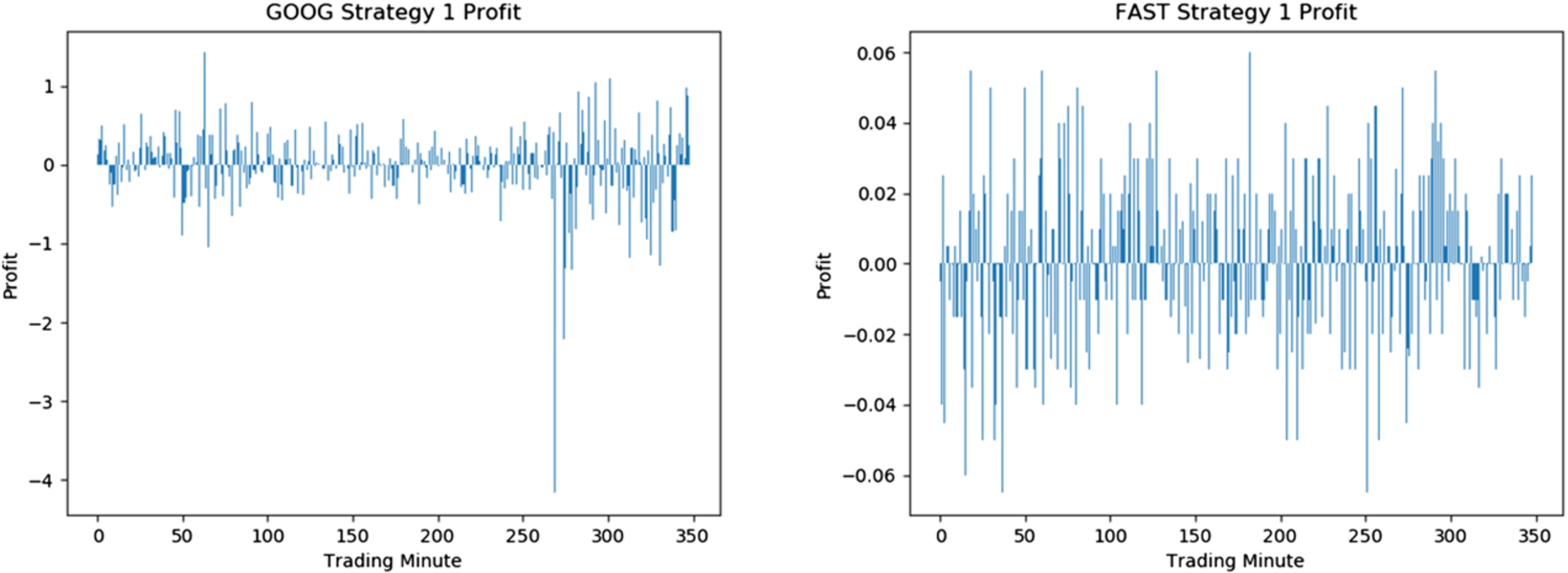
Strategy 1: SS&T profit and loss over time for GOOG and FAST stocks.

Fig. 10.

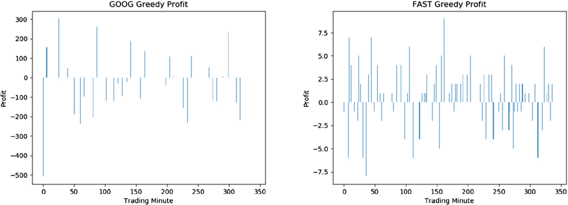
Strategy 2: Greedy strategy profit and loss over time for GOOG and FAST stocks.

Fig. 11.

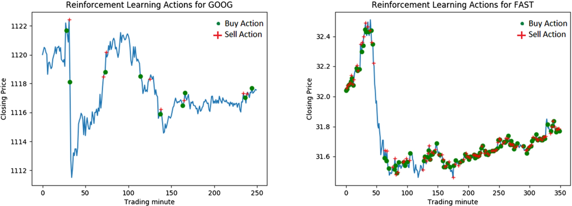
Strategy 3: Reinforcement learning buy and sell operations over time.

In Table 5, we compare the profits from our profit enhancement techniques to two baselines. The prediction model that is used for our two profit computation strategies (SS&T and Greedy) is $LSTM + VAE + AVG$ . We select this model for the computation of profit on the basis of its superior performance in terms of accuracy, which is tabulated in Table 4. For Prophet, we use the SS&T method for the computation of profit and the results indicate that our model shows higher profitability for all the 12 tickers. The buy and hold (B&H) baseline is inferior to the SS&T technique for all the 12 tickers but gives better performance than the Greedy strategy or the reinforcement learning strategy for some of the tickers. However, in case of buy and hold, the profit is totally dependent on the specific test set and the difference between the price of the first minute of the test set and the last minute of the test set. On the other hand, the greedy strategy and the reinforcement learning strategy can make a profit by buying and selling stocks throughout the time interval covered by the test set and is not wholly dependent on two specific values in the test set.

By comparing the profits from SS&T and Greedy strategies, we find that in most cases, the SS&T strategy shows better performance. However, it is worthwhile to note that the SS&T strategy involves the use of short selling, which is not traditionally used but provides better opportunities for earning profit. In case we want to only adhere to traditional stock transactions, the Greedy strategy earns positive profit for 11 out of the 12 selected tickers. In Figs 9 and 10, we show the profit and loss achieved by the SS&T and the Greedy strategies over the same interval of 350 minutes.

On comparing the performance of the reinforcement learning strategy (RL) and the Greedy strategy, we see that the Greedy strategy performs slightly better in most cases, even though the profits of the two strategies are comparable. In case of AMZN and COST tickers, the Greedy strategy performs better and this can be attributed to the use of the predicted future prices. While the reinforcement learning algorithm does not use predicted prices, it shows performance that is comparable to the Greedy strategy and achieves higher profit for AAPL. In Fig. 11, we plot the actual prices for a randomly selected 350 minutes in the test set and the minutes during which buy and sell operations are performed for the GOOG and FAST stocks.

Besides, we also provide two ideal strategies: Greedy-A and DP-Optimal to show the profits that can be earned if we know the future closing prices. In Greedy-A, we identify the profit that our Greedy strategy can earn if it knows the actual closing prices for the next 7 minutes. The DP-Optimal strategy assumes that the algorithm knows the entire future closing prices for the whole test set at the very beginning and can decide when to buy and sell stocks on that basis. This is the maximum possible profit that can be earned over the period of time covered by the test set by making at most 1 transaction per minute. These strategies show superior performance to all others but are only provided to emphasize the importance of accurate future predictions, which is difficult in case of stock prices due to the inherent randomness of the data. In reality, we can never use the Greedy-A and the DP-Optimal strategy because the actual future stock prices are always unknown.

8. Conclusion and future work

The goal of this paper is to address the problem of high frequency stock price predictions from historical prices and to improve upon the state-of-the-art techniques of time-series prediction of stock prices by proposing a deep learning framework. Our framework takes minutely data for 12 different stocks tickers and predicts the stock closing price for 7-minute-ahead. In our framework, before feeding the minute data to a prediction model, we remove noise from the data by using a Variational Autoencoder and explore the use of time series feature extraction techniques to map the data into a high dimensional feature space. The new set of features are fed to a stacked LSTM Autoencoder to predict the deviation of the stock closing price for the next 7 minutes from the average closing price of the last 7 minutes. Two profit enhancement strategies are applied based on this prediction to provide advice to the users about the appropriate time for buying or selling a stock. Besides, we use reinforcement learning to build a third profit enhancement strategies. Our results show that our proposed models beat the state-of-the-art approach in the area of time series forecasting and profitability. The increased profit from our models is due to the higher accuracy of prediction. This fact is corroborated by the much higher profits achieved by the offline models that use the actual future prices. Our framework paves the way for future research in the field of high frequency stock price predictions by providing valuable insights for noise removal, price prediction and profit enhancement as well as by identifying the challenges of performing hyper-parameter optimization on data that involves some randomness.

We will analyze our frameworks on the top 100 NASDAQ stocks in the near future. There are many avenues for improvement in our work. We could incorporate real time sentiment analysis of news. It would be interesting to find out if models that predict seconds, minutes, and hourly data, can be ensembled to produce better models. Optimizing time of model building is another area that needs further research.

References

Abrishami,

Turek,

Roy Choudhury and

Kumar, Enhancing profit by predicting stock prices using deep neural networks, in: 2019 IEEE 31st International Conference on Tools with Artificial Intelligence (ICTAI), 2019.

Akhauri, TradeBot: Stock trading using reinforcement learning – Part 1, 2019, https://medium.com/ether-labs/tradebot-stock-trading-using-reinforcement-learning-part1-8b67c9603f33/.

M.F.

Association, An introduction to short selling, 2018, http://hedgefundamentals.org/wp-content/uploads/2018/05/An-Introduction-to-Short-Selling_White-Paper.pdf/.

G.S.

Atsalakis and

K.P.

Valavanis, Surveying stock market forecasting techniques – Part II: Soft computing methods, Expert Syst. Appl. 36(3) (2009), 5932–5941. doi:10.1016/j.eswa.2008.07.006.

A.R.

Azhikodan,

A.G.K.

Bhat and

M.V.

Jadhav, Stock trading bot using deep reinforcement learning, in: Innovations in Computer Science and Engineering,

H.S.

Saini,

Sayal,

Govardhan and

Buyya, eds, Springer, Singapore, Singapore, 2019, pp. 41–49. ISBN 978-981-10-8201-6. doi:10.1007/978-981-10-8201-6_5.

Bao,

Yue and

Rao, A deep learning framework for financial time series using stacked autoencoders and long-short term memory, PloS one 12(7) (2017), e0180944. doi:10.1371/journal.pone.0180944.

Batal and

Hauskrecht, A supervised time series feature extraction technique using DCT and DWT, in: 2009 International Conference on Machine Learning and Applications, IEEE, 2009, pp. 735–739. doi:10.1109/ICMLA.2009.13.

Bergstra,

Yamins and

D.D.

Cox, Making a science of model search, CoRR, 2012 arXiv:1209.5111.

Chou and

Nguyen, Forward forecast of stock price using sliding-window metaheuristic-optimized machine-learning regression, IEEE Transactions on Industrial Informatics 14(7) (2018), 3132–3142. doi:10.1109/TII.2018.2794389.

10.

Christ,

Braun,

Neuffer and

A.W.

Kempa-Liehr, Time series FeatuRe extraction on basis of scalable hypothesis tests (tsfresh – A Python package), Neurocomputing 307 (2018), 72–77. doi:10.1016/j.neucom.2018.03.067.

11.

S.P.

Das and

Padhy, Support vector machines for prediction of futures prices in Indian stock market, International Journal of Computer Applications 41(3) (2012).

12.

B.U.

Devi,

Sundar and

Alli, An effective time series analysis for stock trend prediction using ARIMA model for nifty midcap-50, International Journal of Data Mining & Knowledge Management Process 3(1) (2013), 65. doi:10.5121/ijdkp.2013.3106.

13.

Ding,

Zhang,

Liu and

Duan, Deep learning for event-driven stock prediction, in: Twenty-Fourth International Joint Conference on Artificial Intelligence, 2015.

14.

Ganesh and

Rakheja, Deep reinforcement learning in high frequency trading, CoRR, 2018, arXiv:1809.01506.

15.

S.S.

Groth and

Muntermann, An intraday market risk management approach based on textual analysis, Decision Support Systems 50(4) (2011), 680–691. doi:10.1016/j.dss.2010.08.019.

16.

Guo,

Wang,

Liu and

Yang, A feature fusion based forecasting model for financial time series, PloS one 9(6) (2014), e101113. doi:10.1371/journal.pone.0101113.

17.

Guyon,

Weston,

Barnhill and

Vapnik, Gene selection for cancer classification using support vector machines, Machine Learning 46(1) (2002), 389–422. doi:10.1023/A:1012487302797.

18.

Hochreiter and

Schmidhuber, Long short-term memory, Neural Comput. 9(8) (1997), 1735–1780. doi:10.1162/neco.1997.9.8.1735.

19.

IG , What causes share prices to change? 2020.

20.

Investopedia, Technical analysis.

21.

J.E.

Jarrett and

Kyper, ARIMA modeling with intervention to forecast and analyze Chinese stock prices, International Journal of Engineering Business Management 3 (2011), 17. doi:10.5772/50938.

22.

Khan,

Aadil,

M.A.

Ghazanfar,

Khan,

Metawa,

Muhammad,

Mehmood and

Nam, A robust regression-based stock exchange forecasting and determination of correlation between stock markets, Sustainability 10(10) (2018), 3702, https://www-mdpi-com-s.web.bisu.edu.cn/2071-1050/10/10/3702 . doi:10.3390/su10103702.

23.

D.P.

Kingma and

Welling, Auto-encoding variational Bayes, arXiv e-prints, 2013, arXiv:1312.6114.

24.

Krollner,

Vanstone and

Finnie, Financial time series forecasting with machine learning techniques: A survey, in: Proceedings of the 18th European Symposium on Artificial Neural Networks (ESANN 2010), 2010, pp. 25–30. ISBN 2930307102.

25.

Kuremoto,

Kimura,

Kobayashi and

Obayashi, Time series forecasting using a deep belief network with restricted Boltzmann machines, Neurocomputing 137 (2014), 47–56. doi:10.1016/j.neucom.2013.03.047.

26.

Li, Deep reinforcement learning: An overview, CoRR, 2017, arXiv:1701.07274.

27.

C.-J.

Lu,

T.-S.

Lee and

C.-C.

Chiu, Financial time series forecasting using independent component analysis and support vector regression, Decision Support Systems 47(2) (2009), 115–125. doi:10.1016/j.dss.2009.02.001.

28.

Malhotra,

Ramakrishnan,

Anand,

Vig,

Agarwal and

Shroff, LSTM-based encoder–decoder for multi-sensor anomaly detection, CoRR, 2016, arXiv:1607.00148.

29.

Meyer,

Beutel and

Thiele, Unsupervised feature learning for audio analysis, CoRR, 2017, arXiv:1712.03835.

30.

Park,

Hoshi and

C.C.

Kemp, A multimodal anomaly detector for robot-assisted feeding using an LSTM-based variational autoencoder, IEEE Robotics and Automation Letters 3(3) (2018), 1544–1551. doi:10.1109/LRA.2018.2801475.

31.

Rama and

Ç.

Çöltekin, LSTM autoencoders for dialect analysis, in: Proceedings of the Third Workshop on NLP for Similar Languages, Varieties and Dialects (VarDial3), The COLING 2016 Organizing Committee, Osaka, Japan, 2016, pp. 25–32, https://www.aclweb.org/anthology/W16-4803 .

32.

A.M.

Rather,

Agarwal and

Sastry, Recurrent neural network and a hybrid model for prediction of stock returns, Expert Systems with Applications 42(6) (2015), 3234–3241. doi:10.1016/j.eswa.2014.12.003.

33.

Rundo,

Trenta,

A.L.

Di Stallo and

Battiato, Advanced Markov-based machine learning framework for making adaptive trading system, Computation 7(1) (2019), 4, https://www-mdpi-com-s.web.bisu.edu.cn/2079-3197/7/1/4 . doi:10.3390/computation7010004.

34.

R.P.

Schumaker,

Zhang,

C.-N.

Huang and

Chen, Evaluating sentiment in financial news articles, Decis. Support Syst. 53(3) (2012), 458–464. doi:10.1016/j.dss.2012.03.001.

35.

scikit-learn developers (BSD License), sklearn.preprocessing.MinMaxScaler, 2018.

36.

Shen,

Jiang and

Zhang, Stock market forecasting using machine learning algorithms, Department of Electrical Engineering, Stanford, CA, 2012, pp. 1–5.

37.

Srivastava,

Mansimov and

Salakhutdinov, Unsupervised learning of video representations using LSTMs, CoRR, 2015, arXiv:1502.04681.

38.

Straburg,

Gonzalez-Martel and

Alexandrov, Parallel genetic algorithms for stock market trading rules, Procedia Computer Science 9 (2012), 1306–1313. doi:10.1016/j.procs.2012.04.143.

39.

Sutskever,

Vinyals and

Q.V.

Le, Sequence to sequence learning with neural networks, CoRR, 2014, arXiv:1409.3215.

40.

F.E.

Tay and

Cao, Application of support vector machines in financial time series forecasting, omega 29(4) (2001), 309–317. doi:10.1016/S0305-0483(01)00026-3.

41.

S.J.

Taylor and

Letham, Forecasting at scale, PeerJ Preprints 5 (2017), e3190v1. doi:10.7287/peerj.preprints.3190v1.

42.

tradientblog.com, Lessons learned building an ML trading system that turned $5k into $200k, 2019, https://www.tradientblog.com/2019/11/lessons-learned-building-an-ml-trading-system-that-turned-5k-into-200k/.

43.

D.T.

Tran,

Iosifidis,

Kanniainen and

Gabbouj, Temporal attention-augmented bilinear network for financial time-series data analysis, in: IEEE Transactions on Neural Networks and Learning Systems, 2018.

44.

Verleysen and

François, The curse of dimensionality in data mining and time series prediction, in: Proceedings of the 8th International Conference on Artificial Neural Networks: Computational Intelligence and Bioinspired Systems, IWANN’05, Springer-Verlag, Berlin, Heidelberg, 2005, pp. 758–770. ISBN 3-540-26208-3, 978-3-540-26208-4. doi:10.1007/11494669_93.

45.

Wang,

Huang and

Wang, A novel text mining approach to financial time series forecasting, Neurocomputing 83 (2012), 136–145. doi:10.1016/j.neucom.2011.12.013.

46.

C.J.C.H.

Watkins, Learning from delayed rewards, PhD thesis, King’s College, Cambridge, UK, 1989, http://www.cs.rhul.ac.uk/~chrisw/new_thesis.pdf.

47.

Wei,

Wu and

Ma, An AutoEncoder and LSTM-based traffic flow prediction method, Sensors 19 (2019), 2946. doi:10.3390/s19132946.

48.

Xiong,

Liu,

Zhong,

Yang and

Walid, Practical deep reinforcement learning approach for stock trading, CoRR, 2018, arXiv:1811.07522.

49.

Zhang,

Zhou,

Pan,

Hu,

Tang and

Zhao, Stock market prediction on high-frequency data using generative adversarial nets, Mathematical Problems in Engineering 7 (2018), 4907423. doi:10.1155/2018/4907423.

50.

Zhao,

Rao,

Tu and

Shi, Time-weighted LSTM model with redefined labeling for stock trend prediction, in: 2017 IEEE 29th International Conference on Tools with Artificial Intelligence (ICTAI), 2017, pp. 1210–1217. ISSN 2375-0197. doi:10.1109/ICTAI.2017.00184.

Enhancing profit from stock transactions using neural networks

Abstract

Keywords

1. Introduction

3. Data description

Table 1 Iexfinance stock data sample features and their descriptions Feature Description marketOpen First price for the minute. marketHigh Highest price for the minute. marketLow Lowest price for the minute. marketClose Last price for the minute. marketvolume Total volume of trades for the minute.

4.1. Data normalization and preparation

4.1.1. Data normalization

4.1.2. Restructuring of data into input and output windows

4.1.3. Pre-processing to enable closing price deviation prediction

4.2. Feature engineering and variational autoencoder

4.2.1. Variational autoencoder

4 https://tsfresh.readthedocs.io/en/latest/text/introduction.html

5.1. Learning model

6 https://keras.io/

7 http://maxpumperla.github.io/hyperas/

6.1. Strategy 1: Using short selling and traditional transactions (SS&T)

8 https://d2ue93q3u507c2.cloudfront.net/assets/robinhood/legal/RHF%20Retail%20Commissions%20and%20Fees%20Schedule.pdf

6.4. Offline strategies

6.4.1. Offline greedy strategy (Greedy-O)

6.4.2. Offline dynamic programming (DP-O)

7. Experimental results

7.1. Data splits, baseline and forecasting models

9 https://facebook.github.io/prophet/

10 https://www.statisticshowto.datasciencecentral.com/probability-and-statistics/coefficient-of-determination-r-squared/

References

⁴
https://tsfresh.readthedocs.io/en/latest/text/introduction.html

⁶
https://keras.io/

⁷
http://maxpumperla.github.io/hyperas/

⁸
https://d2ue93q3u507c2.cloudfront.net/assets/robinhood/legal/RHF%20Retail%20Commissions%20and%20Fees%20Schedule.pdf

⁹
https://facebook.github.io/prophet/

¹⁰
https://www.statisticshowto.datasciencecentral.com/probability-and-statistics/coefficient-of-determination-r-squared/