A new stochastic gradient descent possibilistic clustering algorithm

Abstract

Several well known clustering algorithms have their own online counterparts, in order to deal effectively with the big data issue, as well as with the case where the data become available in a streaming fashion. However, very few of them follow the stochastic gradient descent philosophy, despite the fact that the latter enjoys certain practical advantages (such as the possibility of (a) running faster than their batch processing counterparts and (b) escaping from local minima of the associated cost function), while, in addition, strong theoretical convergence results have been established for it. In this paper a novel stochastic gradient descent possibilistic clustering algorithm, called O- ${PCM}_{2}$ is introduced. The algorithm is presented in detail and it is rigorously proved that the gradient of the associated cost function tends to zero in the $L^{2}$ sense, based on general convergence results established for the family of the stochastic gradient descent algorithms. Furthermore, an additional discussion is provided on the nature of the points where the algorithm may converge. Finally, the performance of the proposed algorithm is tested against other related algorithms, on the basis of both synthetic and real data sets.

Keywords

Clustering possibilistic clustering stochastic gradient descent online clustering online k-means

1. Introduction

Cost function minimization is a task that is met in various fields of applications, including data clustering applications, where the associated cost function is defined in terms of all the available data points. Among the most well established methods/algorithms for tackling this task are the iterative ones, where the algorithm initializes the relative parameter vector at a specific value and updates it iteratively, until convergence is achieved. A celebrated iterative cost function minimization method is the gradient descent (GD) one, where at each iteration, the parameter vector is updated, following the opposite direction of the one defined by the gradient of the cost function, computed at the current parameter estimate. By its rationale, it is clear that the GD algorithms may be trapped to local minima of their associated cost function. Moreover, since all the data points contribute to the formation of the gradient at each iteration, several additional issues may arise, including the inability (a) to handle very large data sets (due to memory limitations that do not allow the storage of all the available data points in the memory) and (b) to deal with cases where the data are available in a streaming fashion. One way to face the above issues is to resort to the stochastic rationale, where the parameter updating takes place after the consideration of a single data point drawn randomly from the available data set. The way to utilize the stochastic rationale in the GD context is to approximate the gradient of the cost function (which requires consideration of all data points) with an “instantaneous” gradient, which is computed taking into account only a single (randomly selected) data point. This gives rise to the celebrated stochastic gradient descent (SGD) method, for which several strong theoretical convergence results have been established (e.g., [4,9,14]).

Clustering is the process of partitioning a set of objects into groups so that “more similar” objects are assigned to the same group, while “less similar” objects are assigned to different groups. The resulting groups of this process are called clusters and the set of these clusters constitute the so-called clustering. In most cases, the representation of the objects under study is carried out via the adoption of a set of d suitably chosen features. More specifically, each object $o_{i}$ is represented by a d-dimensional vector, called feature vector consisting of the values these features take for $o_{i}$ (here the case of continuous-valued data is considered). These vectors are called data vectors/points and they constitute the so-called data set. The d-dimensional space, where these vectors live, is called feature space. The degree of similarity between two objects is quantified via a suitably defined proximity measure, computed on their associated feature vectors.

Cost function minimization clustering algorithms is a class of clustering algorithms that has attracted significant attention during the last decades. Here each cluster is modeled by a parameter vector (set of parameters) and an associated cost function is defined, so that its (global) minimum corresponds to values of the parameter vectors that represent the clusters properly. Such algorithms estimate iteratively these parameter vectors through the gradual reduction of the value of their associated cost functions.

The most well studied case is the one where the parameter vectors define points (also called cluster representatives or simply representatives) in the feature space. Assuming that the data points of a cluster are naturally aggregated around a certain data point, its corresponding representative should be located at this point. Several algorithms have been proposed in the above framework, which can be divided into the following general categories, according to the way they define the relation between a data point and a cluster: the hard, the fuzzy and the possibilistic clustering algorithms. The most famous algorithms from the above categories are the k-means [1,6,13], the fuzzy c-means (FCM) [3,7] and the possibilistic c-means (PCMs) [11,12] (algorithms for the case where the clusters are spread around a subspace/affine space of the feature space have also been proposed (subspace clustering, e.g. [16]), but they will not be considered in the present study). In the hard clustering algorithms, each data vector belongs exclusively to a single cluster. In the fuzzy clustering algorithms a certain data vector is shared among all clusters at the same time. The “degree of belongness” of the vector to each cluster is quantified by a number in the interval $[0, 1]$ and these quantities sum up to one. On the other hand, in possibilistic algorithms the relation between a point and a cluster is defined via the notion of “compatibility of the point with the cluster”. That is, for each data vector, although the “degree of compatibility” with each cluster is quantified again by a number in the range $[0, 1]$ , these numbers are not required to sum up to one. Although the sum-to-one constraint is in line with the common intuition, its adoption is not free of problems. Specifically, due to this constraint, both hard and fuzzy clustering (a) require the exact knowledge of the number of clusters (something that, in practice, is rarely known) and (b) they are vulnerable to the presence of noise and outliers. On the other hand, the absence of this constraint from the possibilistic framework abolishes the above problems, at the cost of weaker performance in cases where clusters exhibit significant overlap.

The most well known clustering algorithms of the above general categories perform batch data processing, that is, they update the involved parameters after the processing of the entire data set. However, in order to deal with the case where the data become available in a streaming fashion as well as with the case of large volume data sets, online processing version of the previous algorithms have been developed, e.g., [2] for k-means, [8] for FCM and [18] for PCM. However, only the first one of them follows the stochastic gradient descent philosophy. In the present paper, a stochastic gradient descent possibilistic clustering algorithm, called O- ${PCM}_{2}$ , which has been inspired from the batch possibilistic c-means introduced by Krishnapuram and Keller [12], is proposed. The algorithm enjoys the benefits of both the possibilistic rationale (no need for knowledge of the exact number of clusters, immunity to outliers and noise) and the stochastic gradient descent framework (such as, possibility of faster execution compared to its batch processing counterpart, possibility of escaping from local minima of its associated cost function).

The rest of the paper is organized as follows. Section 2, contains a brief description of the batch possibilistic algorithm [12], as well as a brief presentation of the general stochastic gradient descent scheme. In Section 3, the derivation of the new online possibilistic algorithm O- ${PCM}_{2}$ is carried out. Section 4, contains some mathematical results concerning the convergence behavior of the algorithm. More specifically, it is rigorously proved that the gradient of the cost function associated with O- ${PCM}_{2}$ tends to zero in the $L^{2}$ sense, while a discussion is provided on the nature of the points where the algorithm may converge. In Section 5, the performance of O- ${PCM}_{2}$ is compared to that of other related algorithms, on the basis of both synthetic and real data sets. Finally, Section 6 concludes the paper.

2. Related work

2.1. Batch processing possibilistic clustering

In this subsection, a brief description of the possibilistic c-means algorithm [12], called ${PCM}_{2}$ , is given (this name is to distinguish this algorithm from the first possibilistic algorithm introduced by Krishnapuram and Keller [11]). As is the case for batch processing algorithms, a parameter updating takes place after the consideration of all the available data points. Let X be a data set consisting of N d-dimensional data vectors. That is $\begin{array}{l} X = {x_{i} \in R^{d}, i = 1, \dots, N} \end{array}$ Let $Θ = {θ_{j} \in R^{d}, j = 1, \dots, c}$ , where $θ_{j}$ is the representative of the j-th cluster (which, in the present case, is a point in the space where the data “live”) and c is the number of clusters. Also, let $u_{i j} \in [0, 1]$ be the degree of compatibility of the data point $x_{i}$ with the j-th cluster and let $U = [u_{i j}]$ be the $N \times c$ matrix that accumulates $u_{i j}$ ’s. It is noted that all $u_{i j}$ ’s corresponding to the same vector $x_{i}$ (which occupy the i-th row of U) are independent from each other and they do not necessarily sum to one. The algorithm proposed in [12] is a parametric one (the parameters are the cluster representatives $θ_{j}$ ’s) and it results from the minimization of the following cost function $\begin{array}{l} (1) & J (U, Θ) = \sum_{j = 1}^{c} [\underset{J_{j} (u_{j}, θ_{j})}{\underset{︸}{\sum_{i = 1}^{N} u_{i j} ‖ x_{i} - θ_{j} ‖_{2}^{2} + γ_{j} \sum_{i = 1}^{N} (u_{i j} ln u_{i j} - u_{i j})}}] \end{array}$ where $u_{j}$ is the j-th column of U, which contains the degrees of compatibility of all data vectors with the j-th cluster. Moreover, each $γ_{j}$ is a measure of the variance of the j-th cluster (usually, $γ_{j}$ ’s are user defined, although an adaptive version of PCM, called APCM [17], has been proposed, where they are adapted, as the algorithm evolves).

Equating to zero the gradient of J with respect to U and Θ, respectively, and solving the resulting equations, it turns out that $\begin{array}{l} \frac{\partial J}{\partial u_{i j}} = ‖ x_{i} - θ_{j} ‖_{2}^{2} + γ_{j} ln u_{i j} = 0 \Leftrightarrow \\ (2) & u_{i j} = exp (- \frac{‖ x_{i} - θ_{j} ‖_{2}^{2}}{γ_{j}}), i = 1, \dots, N, j = 1, \dots, c \\ \nabla_{θ_{j}} J \equiv \frac{\partial J}{\partial θ_{j}} = - 2 \sum_{i = 1}^{N} u_{i j} (x_{i} - θ_{j}) = 0 \Leftrightarrow \\ (3) & θ_{j} = \frac{\sum_{i = 1}^{N} u_{i j} x_{i}}{\sum_{i = 1}^{N} u_{i j}}, j = 1, \dots, c \end{array}$ Based on the above equations, ${PCM}_{2}$ initializes $θ_{j}$ ’s and then iterates between (2) and (3) until convergence (that is, until no significant difference is observed between the estimates of $θ_{j}$ ’s obtained in two successive iterations).

In order to initialize the representatives close to dense in data regions, it is suggested to execute the FCM algorithm first with an overestimated number of clusters. The final positions of the representatives resulting by FCM are expected to lie within dense-in-data regions. In addition, due to the overestimated number of clusters, it is very likely to have at least one representative in each dense-in-data region. Then, the final estimates of $θ_{j}$ ’s from FCM, will serve to initialize ${PCM}_{2}$ . With a proper choice of $γ_{j}$ ’s, the algorithm will potentially uncover all the physical clusters, with some of the representatives being (potentially) coincident after the termination of the algorithm (this case arises when two or more representatives were initially located within the same dense-in-data region).

Yang et al. [19] proposed the usage of the same γ for all clusters, i.e., $γ_{j} = γ, j = 1, \dots, c$ . Specifically, the suggested value of γ is given by: $\begin{array}{l} (4) & γ = \frac{β}{q \sqrt{c}} \end{array}$ with $β = \frac{\sum_{i = 1}^{N} ‖ x_{i} - \bar{x} ‖^{2}}{N}, \bar{x} = \frac{\sum_{i = 1}^{N} x_{i}}{N}$ . The term q is a user-defined parameter, which is set to values greater than 1.

It is noticed that the degree of compatibility $u_{i j}$ decreases exponentially fast as the distance between the data vector $x_{i}$ and the representative $θ_{j}$ increases. Thus, even though all the data vectors contribute to the computation of the next position of each $θ_{j}$ , as it is indicated by Eq. (3), the closer the data vector $x_{i}$ is to the corresponding $θ_{j}$ , the greater its influence on the estimation of the next location of $θ_{j}$ . This is the reason why the algorithm eventually moves each representative $θ_{j}$ towards the center of the closer to its initial location dense-in-data region.

Remark 2.1 (Number of clusters).

From equations (2) and (3), it is clear that, for a given $x_{i}$ , the $u_{i j}$ ’s for $j = 1, \dots, c$ are not interrelated and, as a consequence, the $θ_{j}$ ’s are independent from each other. Thus, the minimization of $J (U, Θ)$ can be carried out by minimizing every summand $J_{j} (u_{j}, θ_{j})$ , $j = 1, \dots, c$ independently from the others. As it was stated by Krishnapuram et al. [12], a consequence of the independence among the $θ_{j}$ ’s is that, for a proper choice of $γ_{j}$ ’s, if some of the representatives $θ_{j}$ ’s are initialized close to the same dense-in-data region, their final positions will coincide (usually) to the center of this region (since they do not compete each other), representing all the same cluster. Such representatives may easily be identified after the termination of the algorithm and the duplicates can be removed, in order to keep one representative for each dense region (cluster). This observation indicates that the a priori knowledge of the exact number of clusters is not necessary, for ${PCM}_{2}$ . In general, given an overestimated number of clusters and provided that at least one representative is initialized close to a dense-in-data region, ${PCM}_{2}$ is able to unravel the correct clusters. It is noted that this is not the case with k-means and FCM algorithms, which both require the exact number of clusters, otherwise they give very poor results. For example, if the data points form four physical clusters (that is, we have four aggregations of data points in the associated feature space) and either k-means or FCM are initialized with five clusters, both of them will return five clusters (probably by splitting a physical cluster to two parts). On the other hand, if these algorithms were initialized with three clusters, they would probably merge two physical clusters to one.

Remark 2.2 (Immunity to noise and outliers).

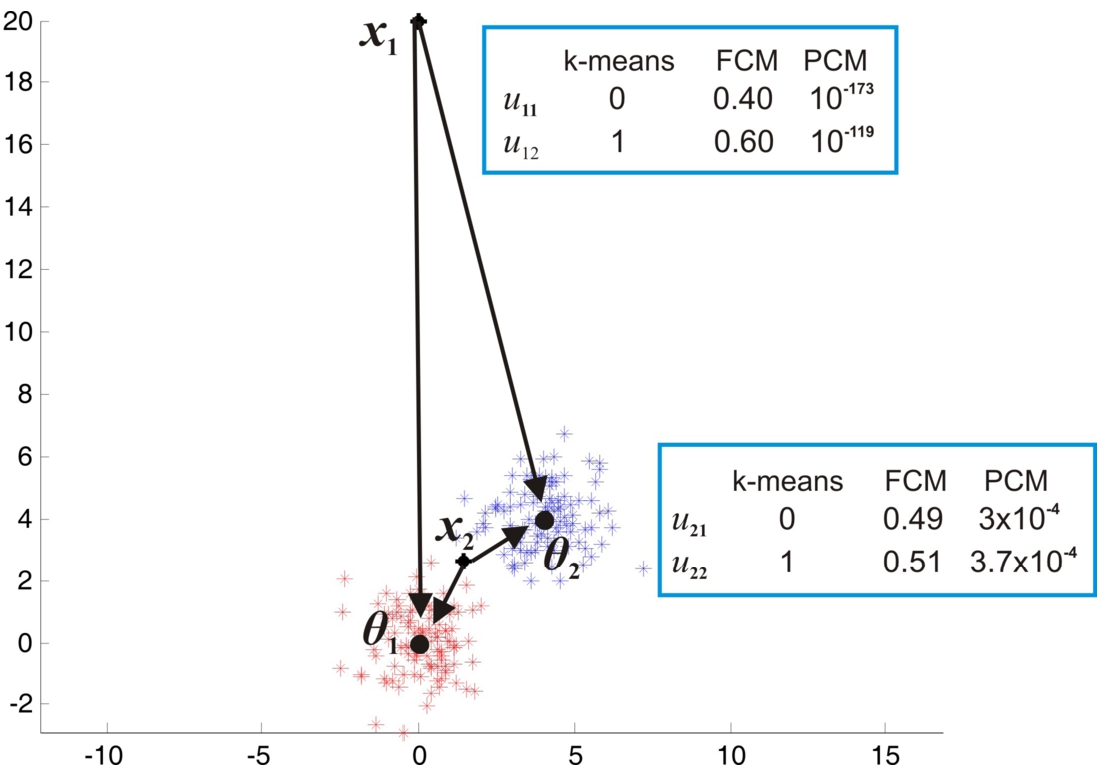
In contrast to k-means and FCM, ${PCM}_{2}$ exhibits high immunity to noise and outliers. This is due to the absence of the sum-to-one constraint. To see this more clearly, consider Fig. 1, where a two-cluster case is shown and a noisy and an outlier points are considered. As it is shown, the $u_{i j}$ coefficients in ${PCM}_{2}$ are substantially lower than those in k-means and FCM, for these points. This implies that these points will have almost no contribution to the estimation of the next values of all $θ_{j}$ ’s (see Eq. (3)), in the context of ${PCM}_{2}$ . On the contrary, they will have a significant contribution to at least one of $θ_{j}$ ’s, in the context of k-means and FCM.

Remark 2.3 (Limitations).

Due to the fact that ${PCM}_{2}$ , as well as k-means and FCM, use single points as cluster representatives, they are suitable to determine only compact and hyperellipsoidally-shaped clusters, while they are not suitable for the determination of other kinds of clusters, e.g., linear clusters (where the data points are spread around a line/line segment in two-dimensional data spaces) and ring-shaped clusters (where the data points lie around a circle). If, in the context of a certain application, one expects other kinds of clusters (e.g., as the above examples), one can still use the hard, the fuzzy and the possibilistic approach, but he/she should parameterize the clusters properly. For example, in the case of line segment shaped clusters, one can adopt line segments as cluster representatives [10] and in the case of ring-shaped clusters one can adopt circles as cluster representatives (e.g., [5]). Of course, in the case where the shape of the clusters is arbitrary, one can resort to non-parametric clustering techniques/algorithms, such as spectral clustering, DBSCAN (e.g. [15]).

All the above characteristics of ${PCM}_{2}$ are inherited to its descendant O- ${PCM}_{2}$ which is introduced in Section 3.

Fig. 1.

The effect of the presence/absence of the sum-to-one constraint, for an outlier ( $x_{1}$ ) and a noisy point ( $x_{2}$ ).

2.2. The stochastic gradient descent (SGD) scheme

The gradient descent (GD) is an iterative cost function minimization scheme, whose associated cost function $F (θ)$ is defined taking into account all the available data points. Specifically, GD updates the estimate of the parameter $θ$ at the t-th iteration, $θ_{t}$ , by following the opposite direction of the gradient of $F (θ)$ computed at $θ_{t}$ , $\nabla_{θ} F (θ_{t})$ . The stochastic gradient descent (SGD) can be viewed as an approximating scheme of GD, since $\nabla_{θ} F$ is replaced by the “instantaneous” gradient computed at a single data point. Let us be more specific. Each SGD algorithm is associated with a loss function $f (θ; x_{i})$ , calculated on a certain data vector $x_{i}$ and an objective function, which is the mean of the loss function values computed on each data vector. More specifically, the associated objective function can be defined as $\begin{array}{l} (5) & F (θ) : = \frac{1}{N} \sum_{i = 1}^{N} f (θ; x_{i}) \end{array}$ Denoting by $\nabla f (θ_{t}; x)$ the gradient of $f (θ; x)$ with respect to $θ$ , computed at $θ = θ_{t}$ , the general SGD scheme is given below

Stochastic Gradient Descent – SGD

Input: X

Initialization: Initialize $θ$ to $θ_{0}$

$t = 0$

Repeat

Pick at random a sample point $x_{t}$ from X

Compute $\nabla f (θ_{t}; x_{t})$

Compute $a_{t}$

Update $θ_{t + 1} = θ_{t} - a_{t} \nabla f (θ_{t}; x_{t})$

$t = t + 1$

Until a termination criterion is met

Output: $θ$

The sequence $a_{t}$ , called learning rate sequence, is a deterministic sequence, which tends to 0, as $t \to + \infty$ . If, in addition, it fulfills some additional conditions (see below), certain convergence results can be established for SGD scheme .1

¹
In some cases the learning rate can be fixed to a small value. In this case, the algorithm reaches close to the minimum of the cost function and oscillates around it.

Among the advantages of SGD scheme are (a) its ability to deal well with very large data sets, since only a single data point is processed at each iteration, (b) its ability of escaping from local minima of the associated cost function, due to the oscillations introduced by the processing of each individual data point and (c) its ability to converge much faster than the corresponding batch GD scheme in the case of large data sets, where a lot of redundant information is encountered among the data points. On the other hand, the weak points of SGD include (a) the possibility of diverging towards a wrong direction, due to the oscillations introduced by the separate processing of each data point, (b) the larger (in some cases) time needed for convergence, due to oscillation phenomena around the solution and (c) the loss of the ability to take advantage of the performance of vectorized operations. One way to keep the advantages of SGD and to alleviate (to a certain degree) its disadvantages, is the adoption of the mini batch rationale, where a small number of data points is processed simultaneously (e.g., [4]).

3. The O-

{PCM}_{2}

algorithm

In contrast to the batch processing framework (see Section 2.1), in the online processing, the values of U are not of significant value anymore, since they are computed based only on the data points processed so far. The only useful information now is about $θ_{j}$ ’s, which identify the location of the clusters in the data space. The assignment of the data points to clusters can take place after the determination of the final locations of the $θ_{j}$ ’s. More specifically, each data vector $x_{i}$ can be assigned to the cluster associated with the representative that lies closest to $x_{i}$ . Based on the above observation, the clustering algorithm should be designed so that to determine only the locations of $θ_{j}$ ’s. Thus, it is reasonable to define an objective function, which does not contain the terms $u_{i j}$ ’s. One way to do this is to substitute in the formula of $J (U, Θ)$ given in Eq. (1), the $u_{i j}$ ’s with their optimal (in the batch case) values given in Eq. (2). Thus, defining $U^{*} = {[u_{i j}]}_{N \times c}$ , where $u_{i j} = exp (- \frac{‖ x_{i} - θ_{j} ‖_{2}^{2}}{γ_{j}})$ , $i = 1, \dots, N, j = 1, \dots, c$ , and after some algebra, it follows that $\begin{array}{l} (6) & J^{*} (Θ) : = J (U^{*}, Θ) = - \sum_{j = 1}^{c} γ_{j} \sum_{i = 1}^{N} exp (- \frac{‖ x_{i} - θ_{j} ‖_{2}^{2}}{γ_{j}}) = \sum_{i = 1}^{N} [- \sum_{j = 1}^{c} γ_{j} exp (- \frac{‖ x - θ_{j} ‖_{2}^{2}}{γ_{j}})] \end{array}$

The above expression indicates the following loss function $\begin{array}{l} (7) & f_{OPCM 2} (Θ; x) = - \sum_{j = 1}^{c} γ_{j} exp (- \frac{‖ x - θ_{j} ‖_{2}^{2}}{γ_{j}}) \end{array}$ whose corresponding objective/risk function is $\begin{array}{l} (8) & F_{OPCM 2} (Θ) : = \frac{1}{N} \sum_{i = 1}^{N} f_{OPCM 2} (Θ; x_{i}) = \sum_{j = 1}^{c} \underset{F_{j} (θ_{j})}{\underset{︸}{[- \frac{1}{N} γ_{j} \sum_{i = 1}^{N} exp (- \frac{‖ x_{i} - θ_{j} ‖_{2}^{2}}{γ_{j}})]}} \end{array}$

Taking the gradient of the loss function given in Eq. (7) with respect to $θ_{j}$ , it follows that $\begin{array}{l} (9) & \nabla_{θ_{j}} f_{OPCM 2} = - 2 exp (- \frac{‖ x - θ_{j} ‖_{2}^{2}}{γ_{j}}) (x - θ_{j}) \end{array}$ Hence, in the spirit of the SGD scheme, the following updating rule results, for $j = 1, \dots, c$ : $\begin{array}{l} (10) & θ_{j}^{(t + 1)} = θ_{j}^{(t)} + 2 a_{j}^{(t)} exp (- \frac{‖ x_{t} - θ_{j}^{(t)} ‖_{2}^{2}}{γ_{j}}) (x_{t} - θ_{j}^{(t)}) \end{array}$ where $a_{j}^{(t)}, t \in N, j = 1, \dots, c$ are the sequences of learning rates, each one corresponding to a cluster, which must satisfy certain conditions to guarantee convergence (they are given in the next section). In order to lighten the notation, the time index will be given as subscript in the absence of any other index.

Having said all the above, it is presented next the proposed online version of ${PCM}_{2}$ algorithm (O- ${PCM}_{2}$ algorithm). The inputs of the algorithm are the dataset X, the number of clusters c (usually, the algorithm is initialized with an overestimated number of clusters) and the parameter γ (in general, one value for each cluster). The algorithm in each iteration selects at random and with replacement a data point $x_{t}$ from the entire data set X and updates all the representatives $θ_{j}$ ’s, $j = 1, \dots, c$ utilizing Eq. (10). The algorithm is terminated, when a certain termination criterion is met. For example when the euclidean norm of the distance between two successive positions of the representatives is less than a (small) user defined parameter, the tolerance. Finally, the final positions of the representatives of the clusters are returned as output of the algorithm (no matrix U is returned). O- ${PCM}_{2}$ can be written as follows:

Online ${PCM}_{2}$ –O- ${PCM}_{2}$

Input: X, c, $γ_{j}$ , $j = 1, \dots, c$

Initialization: Initialize $θ_{j} \equiv θ_{j}^{(0)}, j = 1, \dots, c$

$t = 0$

Repeat

Pick at random a sample point $x_{t}$ from X

For $j = 1$ to c

Compute $u_{j}^{(t)} = exp (- \frac{‖ x_{t} - θ_{j}^{(t)} ‖_{2}^{2}}{γ_{j}})$

Compute $a_{j}^{(t)}$

Update $θ_{j}^{(t + 1)} = θ_{j}^{(t)} + a_{j}^{(t)} \cdot 2 u_{j}^{(t)} (x_{t} - θ_{j}^{(t)})$

$t = t + 1$

Until a termination criterion is met

Output: Θ

4. Convergence analysis of O- ${PCM}_{2}$

In this section, the focus is on the convergence of the O- ${PCM}_{2}$ algorithm. More specifically, it will be proved rigorously that the gradient of the objective function F converges (in the $L^{2}$ sense) to $0$ , utilizing some general convergence results for the stochastic gradient descent (SGD) algorithms [4]. Then, a qualitative discussion follows on the nature of the points where O- ${PCM}_{2}$ may converge.

Before the detailed presentation of the above results, the general convergence results on SGD algorithms on which the proof of the convergence of O- ${PCM}_{2}$ is based, are briefly presented.

4.1. Convergence result for the SGD scheme

In the following, some convergence results for the general SGD scheme are provided, for the case where $\nabla f (θ_{t}, x_{t})$ is an unbiased estimator of $\nabla F (θ_{t})$ (note that O- ${PCM}_{2}$ exhibits this property). These results can be extracted from more general results given in [4], thus no proofs will be provided for them.

Assumption 4.1.
(a) The objective function $F : R^{d} \to R$ is continuously differentiable and (b) the gradient of F, namely $\nabla F : R^{d} \to R^{d}$ , is Lipschitz continuous with Lipschitz constant $L > 0$ , i.e. $\begin{matrix} {‖ \nabla F (θ) - \nabla F (\tilde{θ}) ‖}_{2} ⩽ L ‖ θ - \tilde{θ} ‖_{2}, \forall θ, \tilde{θ} \in R^{d} \end{matrix}$

This assumption ensures that the gradient of F does not change arbitrarily quickly with respect to the parameter vector $θ$ .

In the following, the expectation and variance operators are defined over the distribution of $x_{t}$ given $θ_{t}$ .
Lemma 4.1.
Under Assumption 4.1 , the iterations of the SGD scheme satisfy the following inequality: $\begin{array}{l} (11) & E_{x_{t}} [F (θ_{t + 1})] - F (θ_{t}) ⩽ - a_{t} {‖ \nabla F (θ_{t}) ‖}_{2}^{2} + \frac{1}{2} a_{t}^{2} L E_{x_{t}} [{‖ \nabla f (θ_{t}; x_{t}) ‖}_{2}^{2}] \end{array}$

Note that $F (θ_{t})$ is a deterministic quantity (given $θ_{t}$ ), while $F (θ_{t + 1})$ is of stochastic nature due to the dependence on the randomly selected $x_{t}$ (see Eq. (10)). In addition, if the (deterministic) quantity on the right hand side of the above inequality is manipulated so that to take negative values (this can be achieved by a proper definition of ${a_{t}}$ and if certain conditions are satisfied by $\nabla f (θ; x_{t})$ ), the above lemma guarantees that, in the mean, the value of the objective function exhibits (asymptotically) sufficient decrease.
Assumption 4.2.
The SGD scheme itself and the associated objective function satisfy the following:

(a) the sequence ${θ_{t}}_{t \in N}$ produced by the SGD scheme is contained in an open set over which F is bounded below by a finite value $F_{\min}$

(b) there exist scalars $M ⩾ 0, M_{v} ⩾ 0$ so that for all t it is $\begin{array}{l} (12) & V_{x_{t}} [\nabla f (θ_{t}; x_{t})] ⩽ M + M_{v} {‖ \nabla F (θ_{t}) ‖}_{2}^{2} \end{array}$ where the variance of $\nabla f (θ_{t}; x_{t})$ , $V_{x_{t}} [\nabla f (θ_{t}; x_{t})]$ , is defined as $\begin{array}{l} (13) & V_{x_{t}} [\nabla f (θ_{t}; x_{t})] : = E_{x_{t}} [{‖ \nabla f (θ_{t}; x_{t}) ‖}_{2}^{2}] - {‖ E_{x_{t}} [\nabla f (θ_{t}; x_{t})] ‖}_{2}^{2} \end{array}$

The Assumption 4.2(b) implies that the variance of $\nabla f (θ_{t}; x_{t})$ is restricted above by a quadratic function of the norm of the gradient of F.

Combining Eqs (12) and (13) and taking into account the fact that $\nabla f (θ_{t}; x_{t})$ is an unbiased estimator of $\nabla F (θ_{t})$ $(E_{x_{t}} [\nabla f (θ_{t}; x_{t})] = \nabla F (θ_{t}))$ , it follows that $\begin{matrix} E_{x_{t}} [{‖ \nabla f (θ_{t}; x_{t}) ‖}_{2}^{2}] ⩽ M + (M_{v} + 1) {‖ \nabla F (θ_{t}; x_{t}) ‖}_{2}^{2} . \end{matrix}$

The latter combined with Eq. (11), and after some algebra, gives $\begin{array}{l} (14) & E_{x_{t}} [F (θ_{t + 1})] - F (θ_{t}) ⩽ - (1 - \frac{1}{2} a_{t} L (M_{v} + 1)) a_{t} {‖ \nabla F (θ_{t}) ‖}_{2}^{2} + \frac{1}{2} a_{t}^{2} L M \end{array}$

The bound on the right hand side is now a function of $‖ \nabla F (θ_{t}) ‖_{2}^{2}$ and $a_{t}$ . More specifically, the first term in the bound is negative (for small $a_{t}$ ) and proportional to (the deterministic quantity) $‖ \nabla F (θ_{t}) ‖_{2}^{2}$ , while the second term is positive. In order to ensure that the overall bound becomes negative asymptotically, the sequence ${a_{t}}_{t}$ should be properly chosen. It turns out that if
Condition 4.1.
$\sum_{t = 1}^{\infty} a_{t} = \infty, \sum_{t = 1}^{\infty} a_{t}^{2} < \infty$ this aim is achieved.

The combination of all the above ingredients leads to the following general convergence result [4]:
Theorem 4.1.
Under Assumptions 4.1 and 4.2 , suppose that the SGD algorithm is run with a stepsize sequence ${a_{t}}_{t \in N}$ , which satisfies Condition 4.1 . If in addition (a) the objective function F is twice differentiable, and (b) the mapping $θ \to ‖ \nabla F (θ) ‖_{2}^{2}$ has Lipschitz-continuous derivatives, then $\begin{array}{l} lim_{t \to \infty} E [{‖ \nabla F (θ_{t}) ‖}_{2}^{2}] = 0 \end{array}$ where $E$ denotes the expected value taken with respect to the joint distribution of all the random variables ${x_{t}}_{t \in N}$ .

Having presented in brief the general theoretical framework that fits to O- ${PCM}_{2}$ , the proof of convergence of O- ${PCM}_{2}$ is provided next.
4.2. Convergence proof of O- ${PCM}_{2}$

Before continuing, recall that the representatives $θ_{j}$ ’s $j = 1, \dots, c$ , move independently from each other (as is shown in Eq. (10)). Thus, without loss of generality, the convergence of O- ${PCM}_{2}$ algorithm will be proved for the case of one representative. In this case ( $c = 1$ ), the associated cost function (Eq. (8)) becomes $\begin{array}{l} (15) & F_{OPCM 2} (θ) : = F (θ) = - \frac{1}{N} γ \sum_{i = 1}^{N} exp (- \frac{‖ x_{i} - θ ‖_{2}^{2}}{γ}) \end{array}$

Note that in the above expression the index j, associated with the clusters, is now useless and has been dropped out.

An important note at this point is that $\nabla_{θ} f_{OPCM 2}$ is an unbiased estimator of $\nabla_{θ} F_{OPCM 2}$ , since at each iteration one data point is selected randomly (with replacement) with probability $\frac{1}{N}$ from the entire dataset and thus it is $\begin{matrix} E_{x_{t}} [\nabla f (θ_{t}; x_{t})] = \frac{1}{N} \sum_{i = 1}^{N} \nabla f (θ_{t}; x_{i}) = \nabla F (θ_{t}) . \end{matrix}$

This property allows the use of the theoretical results provided in the previous subsection, in order to establish the convergence results of O- ${PCM}_{2}$ . It is also worth pointing out that the $L^{2}$ norm of the gradient of the objective function F is bounded above by a quadratic function (of course, this holds also for the loss function $f_{OPCM 2}$ ).

Keeping in mind all the above and utilizing Theorem 4.1, it will be proved that for O- ${PCM}_{2}$ it holds that $\begin{matrix} lim_{t \to \infty} E [{‖ \nabla F (θ_{t}) ‖}_{2}^{2}] = 0 . \end{matrix}$

To this end, it will be proved that O- ${PCM}_{2}$ satisfies the requirements of Theorem 4.1.

Next, an important property of the O- ${PCM}_{2}$ algorithm is stated.

Lemma 4.2.
If the stepsize sequence ${a_{t}}_{t \in N}$ satisfies Condition 4.1 , then the sequence of iterations ${θ_{t}}_{t \in N}$ is contained in a bounded set $S$ .
Proof.
The proof follows, if the update rule of O- ${PCM}_{2}$ algorithm is written as: $\begin{matrix} θ_{t + 1} = θ_{t} + a_{t} \cdot 2 u_{t} (x_{t} - θ_{t}) = (1 - 2 a_{t} u_{t}) θ_{t} + 2 a_{t} u_{t} x_{t} . \end{matrix}$

Since the stepsize sequence ${a_{t}}_{t \in N}$ satisfies Condition 4.1, it follows that $a_{t} \overset{t \to \infty}{\to} 0$ , and thus there is a $t_{0} \in N$ such that $a_{t} < \frac{1}{2} \forall t ⩾ t_{0}$ and thus $0 < 2 a_{t} u_{t} < 1 \forall t ⩾ t_{0}$ . This means that the sequence of iterations ${θ_{t}}_{t \in N}$ is contained in the convex hull of $X \cup {θ_{0}, θ_{1}, \dots, θ_{t_{0}}}$ , which is bounded, since the data set X is bounded, as a finite set. □
Remark 4.1.
The assumptions of Theorem 4.1 require specific regularity conditions for the objective function F over the whole $R^{d}$ . However, because the iterations ${θ_{t}}_{t \in N}$ of O- ${PCM}_{2}$ algorithm lie in a bounded domain, call it $S$ , of diameter D (see Lemma 4.2), it is sufficient to prove that F has the required regularity properties only over the set $S$ .

Thus, the regularity properties of F on $S$ will be proved.
Lemma 4.3.
The objective function F of Eq. ( 15 ) satisfies Assumption 4.1 .
Proof.
Clearly, the objective function $F (θ)$ is continuously differentiable. In order to show that the gradient of F is Lipschitz-continuous, it suffices to show that the gradient of $f (θ; x)$ (with respect to $θ$ ) is Lipschitz-continuous. In turn, due to the Mean Value Theorem, it suffices to prove that the functions $\frac{\partial f (θ; x)}{\partial θ_{k}}$ , $k = 1, \dots, d$ have bounded derivatives.

For $k = 1, \dots, d$ , it is $\begin{array}{l} \frac{\partial f (θ; x)}{\partial θ_{k}} = - 2 exp (- \frac{‖ x - θ ‖_{2}^{2}}{γ}) (x_{k} - θ_{k}) = : ϕ_{k} (θ) \end{array}$ The derivatives of $ϕ_{k} (θ)$ , for $k = 1, \dots, d$ , with respect to $θ_{j}, j = 1, \dots, d$ , are $\begin{array}{l} \frac{\partial ϕ_{k} (θ)}{\partial θ_{j}} = - 2 exp (- \frac{‖ x - θ ‖_{2}^{2}}{γ}) (\frac{2}{γ} (x_{k} - θ_{k}) (x_{j} - θ_{j}) - δ_{k j}), \end{array}$ where $δ_{k j} = 1 (0)$ if $k = (\neq) j$ . Thus, $\begin{array}{l} | \frac{\partial ϕ_{k} (θ)}{\partial θ_{j}} | ⩽ | 2 (\frac{2}{γ} (x_{k} - θ_{k}) (x_{j} - θ_{j}) - δ_{k j}) | ⩽ 2 (\frac{2}{γ} D^{2} + 1) \end{array}$ for $j, k = 1, \dots, d$ , since $exp (- \frac{‖ x - θ ‖_{2}^{2}}{γ}) \in (0, 1)$ , and D is the diameter of $S$ . □
Lemma 4.4.
The objective function F of Eq. ( 15 ) and the sequence ${θ_{t}}_{t \in N}$ of O- ${PCM}_{2}$ algorithm satisfy Assumption 4.2 .
Proof.
(a) Based on Lemma 4.2, the sequence of iterations ${θ_{t}}_{t \in N}$ is contained in a bounded set $S$ . Moreover, F is bounded below by $- γ$ .

(b) Since $E_{x_{t}} [\nabla f (θ_{t}; x_{t})] = \nabla F (θ_{t})$ , the variance $V_{x_{t}} [\nabla f (θ_{t}; x_{t})]$ can be written as $\begin{array}{l} V_{x_{t}} [\nabla f (θ_{t}; x_{t})] = E_{x_{t}} [{‖ \nabla f (θ_{t}; x_{t}) ‖}_{2}^{2}] - {‖ \nabla F (θ_{t}) ‖}_{2}^{2} . \end{array}$

In the light of this, it suffices to find $M, M_{V} ⩾ 0$ such that $\begin{array}{l} E_{x_{t}} [{‖ \nabla f (θ_{t}; x_{t}) ‖}_{2}^{2}] ⩽ M + (M_{V} + 1) {‖ \nabla F (θ_{t}) ‖}_{2}^{2} \end{array}$ Recalling that $\nabla f (θ_{t}; x_{t}) = - 2 exp (- \frac{‖ x_{t} - θ_{t} ‖_{2}^{2}}{γ}) (x_{t} - θ_{t})$ , it is easy to verify that for $M = {(2 D)}^{2}$ and $M_{V}$ any non negative number, the above inequality is satisfied. □
Lemma 4.5.
The objective function F of Eq. ( 15 ) is twice differentiable and the mapping $θ \to ‖ \nabla F (θ) ‖_{2}^{2}$ has Lipschitz-continuous derivatives.
Proof.
It is clear that F is twice differentiable. In order to show that the mapping $θ \to ‖ \nabla F (θ) ‖_{2}^{2}$ has Lipschitz-continuous derivatives, let us define the function $F_{1}$ as $\begin{array}{l} F_{1} : = {‖ \nabla F (θ) ‖}_{2}^{2} = \frac{4}{N^{2}} {‖ \sum_{i = 1}^{N} \underset{u_{i} (θ)}{\underset{︸}{exp (- \frac{‖ x_{i} - θ ‖_{2}^{2}}{γ})}} (x_{i} - θ) ‖}_{2}^{2} = \frac{4}{N^{2}} \sum_{k = 1}^{d} {(\sum_{i = 1}^{N} u_{i} (θ) (x_{i k} - θ_{k}))}^{2} \end{array}$ Let $F_{2}$ be the gradient of $F_{1}$ . Then its jth element is $\begin{array}{l} F_{2 j} (θ) = \frac{\partial F_{1} (θ)}{\partial θ_{j}} = \frac{8}{N^{2}} \sum_{k = 1}^{d} [(\sum_{i = 1}^{N} u_{i} (θ) (x_{i k} - θ_{k})) (\sum_{i = 1}^{N} u_{i} (θ) (\frac{2}{γ} (x_{i j} - θ_{j}) (x_{i k} - θ_{k}) - δ_{k j}))] \end{array}$ In order to prove that $F_{2}$ is Lipschitz-continuous, it suffices to show that its derivatives (elements of the respective Hessian matrix) are bounded (over $S$ ). $\begin{array}{l} \frac{\partial F_{2 j}}{\partial θ_{l}} = & \frac{8}{N^{2}} \sum_{k = 1}^{d} [(\sum_{i = 1}^{N} u_{i} (θ) (\frac{2}{γ} (x_{i k} - θ_{k}) (x_{i l} - θ_{l}) - δ_{k l})) (\sum_{i = 1}^{N} u_{i} (θ) (\frac{2}{γ} (x_{i j} - θ_{j}) (x_{i k} - θ_{k}) - δ_{k j}))] \\ + \frac{8}{N^{2}} \sum_{k = 1}^{d} [(\sum_{i = 1}^{N} u_{i} (θ) (x_{i k} - θ_{k})) (\sum_{i = 1}^{N} \frac{2}{γ} u_{i} (θ) (x_{i l} - θ_{l}) (\frac{2}{γ} (x_{i j} - θ_{j}) (x_{i k} - θ_{k}) - δ_{k j}))] \\ - \frac{8}{N^{2}} \sum_{k = 1}^{d} [(\sum_{i = 1}^{N} u_{i} (θ) (x_{i k} - θ_{k})) (\sum_{i = 1}^{N} \frac{2}{γ} u_{i} (θ) (δ_{j l} (x_{i k} - θ_{k}) + δ_{k l} (x_{i j} - θ_{j})))] \end{array}$ for $j, l = 1, \dots, d$ . Since $u_{i} (θ) \in (0, 1)$ and $x_{i}$ ’s and $θ$ live in the bounded set $S$ , (the absolute values of) all the above quantities are bounded. Thus, the $l_{2}$ matrix norm of $\nabla_{θ} (F_{2})$ is bounded over this set and this concludes the proof. □
Theorem 4.2.
Suppose that the O- ${PCM}_{2}$ algorithm is run with a stepsize sequence ${a_{t}}_{t \in N}$ , which satisfies Conditions 4.1 . Then $\begin{array}{l} lim_{t \to \infty} E [{‖ \nabla F (θ_{t}) ‖}_{2}^{2}] = 0 \end{array}$
Proof.
The proof is a direct consequence of Lemmas 4.2, 4.3, 4.4, 4.5 and the Theorem 4.2. □

In words, it has been proved that the gradient of the objective function F converges to $0$ , in the $L^{2}$ sense.
4.3. Qualitative discussion about the convergence points of O- ${PCM}_{2}$

Since the gradient of F over the iterations of O- ${PCM}_{2}$ tends to zero (in the $L^{2}$ sense), it is essential to comment on the nature of the points where O- ${PCM}_{2}$ may converge.

Of course, these points are expected to belong to the set T of points that satisfy $\nabla F (θ) = 0$ , i.e. $T = {θ^{*} : \nabla F (θ^{*}) = 0}$ . Due to the extreme value theorem, whose prerequisites are fulfilled by O- ${PCM}_{2}$ (see Lemma 4.2), the set T is not likely to be empty (due to the form of the cost function, the extreme points are likely to be in the interior of the compact set $S$ ). Thus, T may contain maxima, minima and/or saddle points.

Fig. 2.

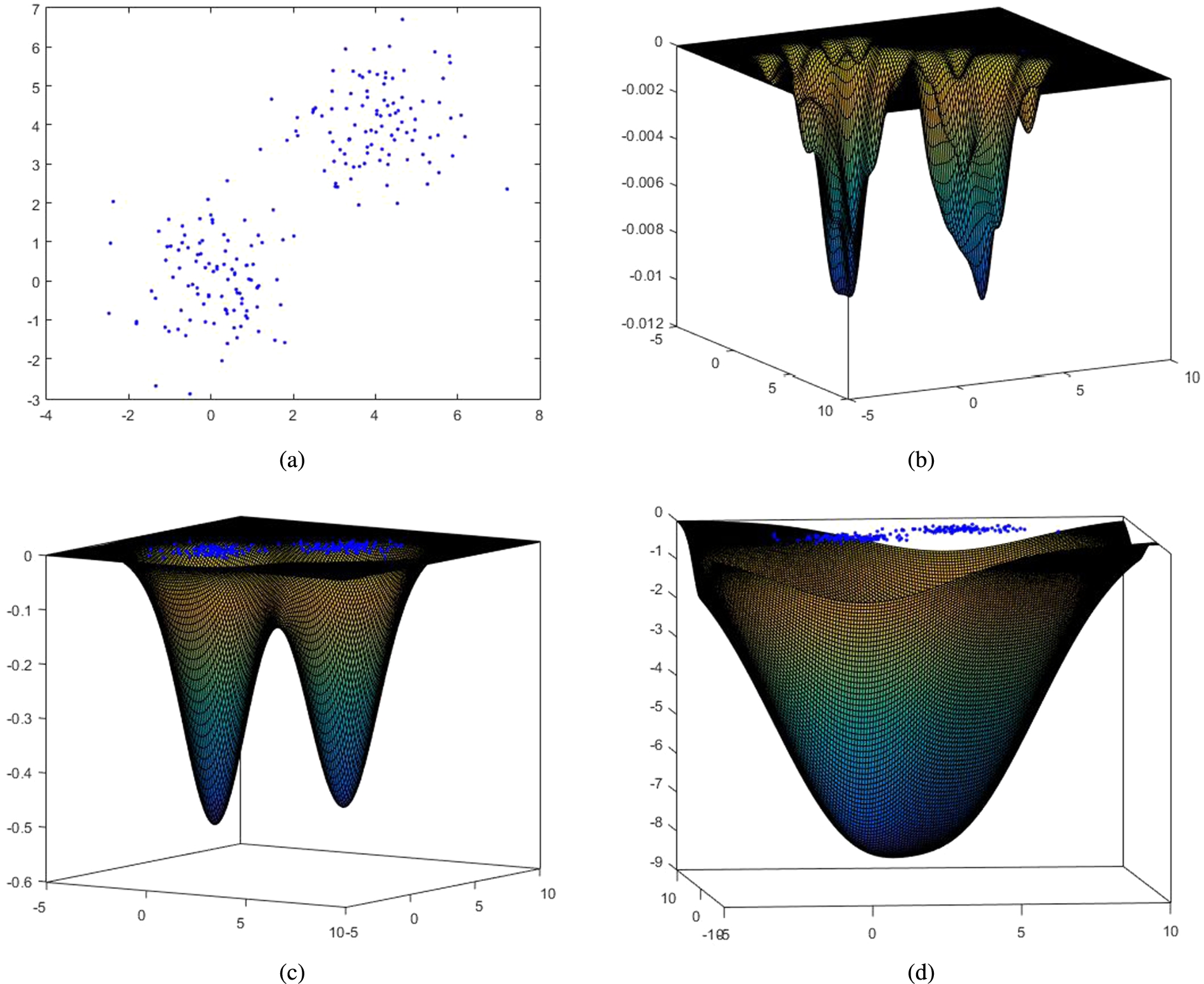
Plot of the cost function F in case of a two-class 2-D dataset. Plot shows (a) the data set and the 3d-plot of function F when (b) $γ = 0.2$ , (c) $γ = 2$ and (d) $γ = 15$ .

Before proceeding any further, let us open a parenthesis in order to gain some insight on the landscape of $F (θ)$ , which depends on the choice of γ, via an example. Let us consider a 2-D data set consisting of two clusters of 100 points each, shown on the xy-plane in Fig. 2(a). The clusters are modeled by normal distributions with means $[0, 0]$ and $[4, 4]$ , respectively, while their covariance matrices are both equal to the identity matrix, $I_{2}$ . As it is illustrated in Fig. 2(b), the function F has more than two local minima, for very small values of the parameter γ. Moreover, as the value of γ increases, the number of local minima decreases, until the function F has only a single (global) minimum (Figs 2(b)–2(d)). It should be noticed that in the cases of Figs 2(b)–2(c), where more than one minima appear, the function F appears to have also saddle points.

Closing the parenthesis, let us now comment on what kind of stationary points of F the O- ${PCM}_{2}$ algorithm can converge. Ineq. (11) (for a proper choice of ${a_{t}}_{t}$ ) guarantees that the algorithm moves towards positions that (in the mean) decrease the cost function asymptotically. Thus, O- ${PCM}_{2}$ cannot converge to a maximum of F. Let us focus now on the other two possible kinds of points in T, that is, the saddle points and the minima points of F.

Let the weighted covariance matrix, associated with a certain $θ$ , be defined as $\begin{array}{l} (16) & Σ (θ) = \frac{\sum_{i = 1}^{N} u_{i} (θ) (x_{i} - θ) {(x_{i} - θ)}^{T}}{\sum_{i = 1}^{N} u_{i} (θ)} \end{array}$

The following Lemma gives a sufficient condition for a $θ^{*} \in T$ to be a local minimum.

Lemma 4.6.

A $θ^{*} \in T$ is a local minima of F if $\begin{array}{l} (17) & λ_{\max}^{*} < \frac{γ}{2} \end{array}$ where $λ_{\max}^{*}$ is the maximum eigenvalue of $Σ (θ^{*})$ .

Proof.

First, the Hessian matrix of F on $θ^{*}$ is computed and then it is examined under which conditions it is positive definite (which implies that $θ^{*}$ is a minimum). It is easy to verify that for any $θ$ , it is $\begin{array}{l} \frac{\partial^{2} F (θ)}{\partial θ_{j}^{2}} = \frac{2}{N} \sum_{i = 1}^{N} u_{i} (θ) - \frac{2}{N} \sum_{i = 1}^{N} \frac{2}{γ} u_{i} (θ) {(x_{i j} - θ_{j})}^{2}, j = 1, \dots, d, \\ \frac{\partial^{2} F (θ)}{\partial θ_{j} \partial θ_{k}} = - \frac{2}{N} \sum_{i = 1}^{N} \frac{2}{γ} u_{i} (θ) (x_{i j} - θ_{j}) (x_{i k} - θ_{k}), j, k = 1, \dots, d, j \neq k . \end{array}$

Combining the above, the Hessian matrix $H (θ)$ can be expressed as $\begin{array}{l} H (θ) = \frac{2}{N} [\sum_{i = 1}^{N} u_{i} (θ) I_{d} - \frac{2}{γ} \sum_{i = 1}^{N} u_{i} (θ) (x_{i} - θ) {(x_{i} - θ)}^{T}] or \\ H (θ) = \frac{2}{N} \sum_{i = 1}^{N} u_{i} (θ) (I_{d} - \frac{2}{γ} Σ (θ)) \end{array}$ where $I_{d}$ is the $d \times d$ identity matrix. Focusing on a $θ^{*} \in T$ , since $Σ (θ^{*})$ is positive (semi) definite, it can be written as $\begin{array}{l} Σ (θ^{*}) = Φ^{*} Λ^{*} {Φ^{*}}^{T} \end{array}$ where $Φ^{*}$ contains in its columns the (orthonormal) eigenvectors of $Σ (θ^{*})$ and $Λ^{*}$ is a diagonal matrix with the eigenvalues $λ_{j}^{*}$ of $Σ (θ^{*})$ in its diagonal. Note also that $Φ^{*} {Φ^{*}}^{T} = I_{d}$ .

In the light of the above, $H (θ^{*})$ becomes $\begin{array}{l} H (θ^{*}) = \frac{2}{N} \sum_{i = 1}^{N} u_{i} (θ^{*}) (Φ^{*} {Φ^{*}}^{T} - \frac{2}{γ} Φ^{*} Λ^{*} {Φ^{*}}^{T}) \\ H (θ^{*}) = \frac{2}{N} \sum_{i = 1}^{N} u_{i} (θ^{*}) Φ^{*} (I_{d} - \frac{2}{γ} Λ^{*}) {Φ^{*}}^{T} \end{array}$

Since $\sum_{i = 1}^{N} u_{i} (θ^{*})$ is positive (due to the definition of $u_{i}$ and the fact that $θ^{*}$ lies in a bounded subset $S$ of $R^{d}$ ), $H (θ^{*})$ is positive definite if $\begin{array}{l} 1 - \frac{2}{γ} λ_{j}^{*} > 0, j = 1, \dots, d or λ_{j}^{*} < \frac{γ}{2} or λ_{\max}^{*} < \frac{γ}{2} \end{array}$ □

The above result is very useful, since it can detect if a stationary point of the cost function, $F (θ)$ , is a local minimum. Let us gain some more insight on the above result recruiting once more the example in Fig. 2(a). We consider the case where γ (which is a measure of the variance of the clusters) is chosen so that $F (θ)$ exhibits as many minima as the number of clusters (see e.g. Fig. 2(c)). Let us consider the center of the first cluster $θ^{*}$ . Then, for the points of this cluster, the $u_{i} (θ^{*})$ ’s will have “large” values, in contrast to the points of the second cluster, which are very “far” from $θ^{*}$ and the respective $u_{i} (θ^{*})$ ’s take very “small” values. Thus, up to a good approximation degree, the contribution of the points from the second cluster to the formation of $Σ (θ^{*})$ can practically be ignored. Therefore, the eigenvalues of $Σ (θ^{*})$ , which measure the spread along the eigenvector directions, will be of the order of γ (since γ is a measure of the variance of the clusters). Of course, similar results hold for points $θ$ that are close to $θ^{*}$ .

Consider now the case where $θ$ lies in the middle of the line segment defined by the centers of the two clusters. In this case, the $u (θ)$ ’s for the points in both clusters are expected to have values of the same order, so all $x_{i}$ ’s from both clusters contribute to the formation of $Σ (θ)$ . Therefore, in this case, $λ_{\max}$ is expected to be very large, compared to γ, since the clusters are distant from each other (as an immediate consequence of the fact that they are well-separated) and, thus, the length of the line segment connecting the centers is significantly greater than γ.

As a conclusion, the result of Lemma 4.6 can be used as a criterion to determine if the point where the algorithm converges is a local minimum of $F (θ)$ , which in the case where γ has been properly chosen, is very likely to correspond to a physical cluster.

5. Experimental results

Although extensive experimentation has been conducted concerning O- ${PCM}_{2}$ , only a limited amount of results is presented here, due to space limitations. In the following experiments, O- ${PCM}_{2}$ is compared with the online k-means algorithm [2], which is of the stochastic gradient descent philosophy, as well as with its batch processing counterpart ${PCM}_{2}$ . The experiments were conducted on both synthetic and real data sets. At each experiment, the number of the initial clusters ( $c_{ini}$ ) for the two possibilistic algorithms is an overestimation of the number of the true clusters (values of $c_{ini}$ close to the chosen ones lead to very similar results). However, for the online k-means, the true number of clusters has been chosen. It is also noted that the sequences $a_{j}^{(t)}$ for O- ${PCM}_{2}$ are chosen as $a_{j}^{(t)} = \frac{1}{2} {(\frac{1}{t})}^{1 / 2 + ε}$ , with $0 < ε ≪ 1$ , a choice that complies with Condition 4.1. Moreover, $θ$ ’s are initialized through FCM applied (a) over the entire set for ${PCM}_{2}$ and (b) over the first 100 randomly selected data points for the online algorithms. Finally, γ’s are defined via Eq. (4).

Experiment 5.1.
The aim of this experiment is to compare the processing time required for the convergence of the three algorithms. Consider the three cluster setup where the clusters stem from three normal distributions with means $μ_{1} = {[1.35, 0.23]}^{'}$ , $μ_{2} = {[4.03, 4.09]}^{'}$ and $μ_{3} = [5.64, 2.28]$ , respectively, while the covariance matrices are all equal to $0.4 I_{2}$ ( $I_{2}$ is the $2 \times 2$ identity matrix). Four data sets are considered, $X_{1}$ , $X_{2}$ , $X_{3}$ , $X_{4}$ , of $N = 1100 \cdot 10^{i - 1}$ data points, $i = 1, 2, 3, 4$ , so that $500 \cdot 10^{i - 1}$ data points are generated from the first distribution (forming the Cluster 1), while $300 * 10^{i - 1}$ data points are generated from each one of the other two distributions (forming Clusters 2 and 3, respectively). Note that clusters $C_{2}$ and $C_{3}$ exhibit partial overlap. The obtained results concerning the computational time required are shown in Table 1. As it can be seen, the processing time for ${PCM}_{2}$ increases rapidly, as the size of the data set increases, while this is not the case with O- ${PCM}_{2}$ and online k-means, with the latter being significantly faster, provided that it has been initialized with the correct number of clusters. It is also worth mentioning the increasing standard deviation associated with the processing time for the online k-means and the O- ${PCM}_{2}$ . This is in line with the fact that the SGD algorithms may sometimes take larger times to converge (see Section 2.2).

Table 1
Results of Experiment 5.1 on the data sets $X_{i}$ , $i = 1, 2, 3, 4$ . The mean execution time along with the standard deviations in parentheses (each experiment run 10 times, except for ${PCM}_{2}$ , which was executed only once due to its batch processing rationale)

Algorithm $c_{ini}$ Time $X_{1}$ Time $X_{2}$ Time $X_{3}$ Time $X_{4}$

${PCM}_{2}$ 10 0.23 1.61 20.23 196.25

O- ${PCM}_{2}$ 10 1.37 (0.68) 1.64 (0.91) 8.31 (4.42) 98.96 (54.72)

Online k-means 3 0.12 (0.05) 0.82 (0.28) 0.83 (0.33) 9.82 (3.25)

Experiment 5.2.
The aim of this experiment is to assess the accuracy of the results of the O- ${PCM}_{2}$ , compared to those of the online k-means and ${PCM}_{2}$ on a more demanding setup. Specifically, consider a five cluster set up, where the clusters are modeled by normal distributions as shown in Table 2. Actually, two data sets, $D_{1}$ and $D_{2}$ , are formed, that differ on their size. The data set $D_{1}$ is depicted in Fig. 3(a). In this case, the accuracy of the results obtained by the algorithms is measured. As in the previous case, there is a bias in favor of the online k-means, since it is initialized with the correct number of clusters. Each experiment has been conducted ten times, with different initializations. The accuracy is assessed in two ways: (a) through the number of times where the clusters were correctly identified (i.e. when at least one $θ_{j}$ is located, after the termination of the algorithm, within the region of a physical cluster) and (b) through the accuracy with which the true cluster centers have been estimated (in terms of the Euclidean distance between the true centers, say $μ_{j}$ ’s, and the respective $θ_{j}$ ’s, after the termination of the algorithms). The results are shown in Table 3.

Table 2
Characteristics of clusters of Experiment 5.2

Cluster Mean Variance $D_{1}$ $D_{2}$

$C_{1}$ $[1, 1]$ $I_{2}$ 4.000 40.000

$C_{2}$ $[4, 4]$ $I_{2}$ 3.000 30.000

$C_{3}$ $[1, 9]$ $0.5 \cdot I_{2}$ 4.000 40.000

$C_{4}$ $[9, 1]$ $1.3 \cdot I_{2}$ 3.000 30.000

$C_{5}$ $[9, 9]$ $0.5 \cdot I_{2}$ 3.000 30.000

Fig. 3.
(a) the physical clusters formed by the points of $D_{1}$ in Experiment 5.2(b) the physical clusters formed by the points of $D_{1}$ plus the 300 noisy points uniformly distributed over the entire region of the space where the data live. (c) the physical clusters formed by the points of $D_{2}$ plus 800 additional points uniformly distributed over the entire region where the points of the $D_{2}$ live.

Table 3
Results of Experiment 5.2 on the data sets $D_{1}$ and $D_{2}$ ( ${PCM}_{2}$ was executed only once due to its batch processing rationale)

Algorithm $c_{ini}$ Perc. of correct $D_{1}$ Accuracy $D_{1}$ Perc. of correct $D_{2}$ Accuracy $D_{2}$

${PCM}_{2}$ 20 1/1 0.0275 1/1 0.0226

O- ${PCM}_{2}$ 20 10/10 0.0944 10/10 0.0897

Online k-means 5 10/10 0.0662 10/10 0.0700

As can be seen from Table 3, all algorithms determine the clusters correctly in all cases, with no significant differences in the accuracy of the estimates of the centers as the volume of the data increases. A similar situation arises, in the presence of uniform noise, as it is shown in the next experiment.
Experiment 5.3.
In this experiment, the behavior of the three algorithms under consideration in a noisy environment, is assessed. Specifically, consider the datasets $D_{1}$ and $D_{2}$ of Experiment 5.2, where 300 and 800 additional data points, respectively, are now inserted randomly as noise in the region of the feature space where the data live (see Figs 3(b)–3(c)). In this case, the obtained results are shown below in Table 4. It can be seen that O- ${PCM}_{2}$ behaves satisfactorily also in a noisy environment. However, it is noted that the accuracy on $D_{1}$ is slightly worse in the case of noise, compared to the non-noisy case, for all algorithms. Interestingly enough, this is not the case with the noisy version of $D_{2}$ , where the ${PCM}_{2}$ and the online k-means perform slightly better performance, compared to the non-noisy version of $D_{2}$ , while the opposite is true for the O- ${PCM}_{2}$ . This is probably due to the randomness that is inherent in the two SGD algorithms.

Table 4
Results of Experiment 5.3 on the data sets $D_{1}$ and $D_{2}$ in the presence of noise

Algorithm $c_{ini}$ Perc. of correct $D_{1}$ Accuracy $D_{1}$ Perc. of correct $D_{2}$ Accuracy $D_{2}$

${PCM}_{2}$ 20 1/1 0.0360 1/1 0.0182

O- ${PCM}_{2}$ 20 10/10 0.1275 10/10 0.1128

Online k-means 5 9/10 0.0856 10/10 0.0643

Fig. 4.
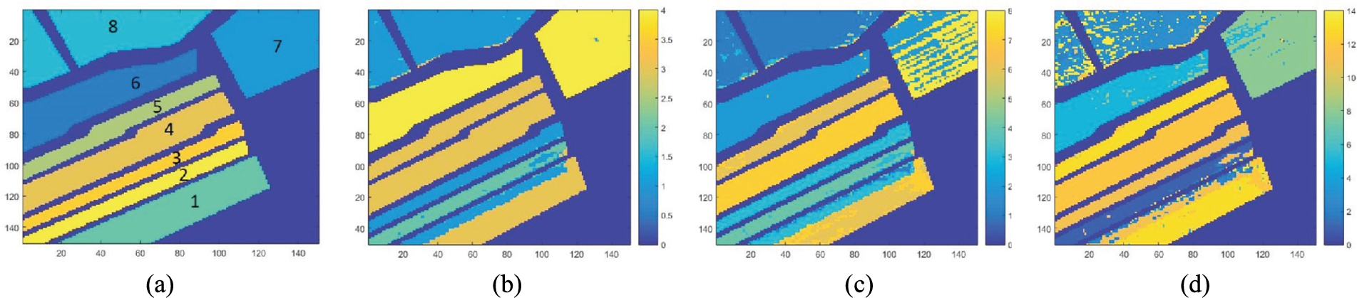
The Salinas experiment. (a) the ground truth information. (b), (c), (d) the results of ${PCM}_{2}$ , online k-means and online ${PCM}_{2}$ , respectively. Note that ${PCM}_{2}$ , recognizes only four distinct clusters.
Experiment 5.4.
This experiment deals with a real application and the aim is to assess the performance of all the algorithms in both a low and a high dimensional version of it. Specifically, in this context, a hyperspectral image, depicting a part of the Salinas valley in California is considered2
²
http://www.ehu.eus/ccwintco/index.php/Hyperspectral_Remote_Sensing_Scenes#Salinas

(Figs 4(a)–4(b)). Each pixel belongs to one out of eight classes corresponding to different cultivations. The size of the image is $150 \times 150$ and the spectral bands are 204. Clustering is performed on the first three principal components of the data set and the agreement of the results with the available ground truth information is measured via the rand measure (RM) (e.g. [15]). The results (Table 5) showed that O- ${PCM}_{2}$ (Fig. 4(c)) gave the best results ( $93 %$ RM), compared to those of ${PCM}_{2}$ ( $82 %$ ) and the online k-means (Fig. 4(d) – $92 %$ ). In addition, it is worth mentioning that the mean execution time for O- ${PCM}_{2}$ with $c_{ini} = 20$ is much smaller than that for the online k-means with $c_{ini} = 8$ (∼ 0.34 secs vs ∼160 secs). Finally, it is noted that O- ${PCM}_{2}$ gave similar results, when it was executed on the original 204-dimensional data, showing that (in principle) it can deal well with high dimensional data.

Table 5
Results of Experiment 5.4

Algorithm $c_{ini}$ $c_{final}$ RM

${PCM}_{2}$ 15 2 57.52

${PCM}_{2}$ 30 4 82.00

O- ${PCM}_{2}$ 15 9 91.82

O- ${PCM}_{2}$ 20 14 93.22

O- ${PCM}_{2}$ 30 17 93.02

Online k-means 3 3 78.12

Online k-means 8 8 92.43

Online k-means 11 11 91.80

Experiment 5.5.
In this experiment, the potential of the O- ${PCM}_{2}$ to deal with dynamically changing environments, is assessed. Such environments are met in applications like motion tracking, where the aim is to detect movement of various objects along the consecutive images (frames) in a video. More specifically, a simple example of a dynamically changing environment is considered here, which involves three clusters of points that move in time (these may correspond to different moving objects).

Fig. 5.
Dynamically changing environment: (a)–(c) three snapshots of the clustering results of O- ${PCM}_{2}$ . (d) the entire movement of the clusters and the $θ$ ’s. The white (black) bullets indicate the final positions of the $θ$ ’s in the first (last) snapshot and the sequence of crosses shows the consecutive positions of $θ$ ’s through time.

At each time snapshot, O- ${PCM}_{2}$ is applied on the current data set (consisting of the clusters formed in the previous snapshot, which now are slightly moved). Considering the data set of the first snapshot, the algorithm runs as usual, while considering every next snapshot, the algorithm is initialized by the values of cluster representatives computed in the previous snapshot. The clustering results of O- ${PCM}_{2}$ in three random snapshots of the experiment are illustrated in Figs 5(a)–5(c). Moreover, the total movement of the data set and the representatives is also shown in Fig. 5(d). As it can be seen, the algorithm behaves very well in this simple example of a dynamically changing environment and thus it seems that, in principle, it has the potential to deal efficiently with such environments.
6. Conclusions

Algorithm	$c_{ini}$	Time $X_{1}$	Time $X_{2}$	Time $X_{3}$	Time $X_{4}$
${PCM}_{2}$	10	0.23	1.61	20.23	196.25
O- ${PCM}_{2}$	10	1.37 (0.68)	1.64 (0.91)	8.31 (4.42)	98.96 (54.72)
Online k-means	3	0.12 (0.05)	0.82 (0.28)	0.83 (0.33)	9.82 (3.25)

Cluster	Mean	Variance	$D_{1}$	$D_{2}$
$C_{1}$	$[1, 1]$	$I_{2}$	4.000	40.000
$C_{2}$	$[4, 4]$	$I_{2}$	3.000	30.000
$C_{3}$	$[1, 9]$	$0.5 \cdot I_{2}$	4.000	40.000
$C_{4}$	$[9, 1]$	$1.3 \cdot I_{2}$	3.000	30.000
$C_{5}$	$[9, 9]$	$0.5 \cdot I_{2}$	3.000	30.000

Algorithm	$c_{ini}$	Perc. of correct $D_{1}$	Accuracy $D_{1}$	Perc. of correct $D_{2}$	Accuracy $D_{2}$
${PCM}_{2}$	20	1/1	0.0275	1/1	0.0226
O- ${PCM}_{2}$	20	10/10	0.0944	10/10	0.0897
Online k-means	5	10/10	0.0662	10/10	0.0700

Algorithm	$c_{ini}$	Perc. of correct $D_{1}$	Accuracy $D_{1}$	Perc. of correct $D_{2}$	Accuracy $D_{2}$
${PCM}_{2}$	20	1/1	0.0360	1/1	0.0182
O- ${PCM}_{2}$	20	10/10	0.1275	10/10	0.1128
Online k-means	5	9/10	0.0856	10/10	0.0643

Algorithm	$c_{ini}$	$c_{final}$	RM
${PCM}_{2}$	15	2	57.52
${PCM}_{2}$	30	4	82.00
O- ${PCM}_{2}$	15	9	91.82
O- ${PCM}_{2}$	20	14	93.22
O- ${PCM}_{2}$	30	17	93.02
Online k-means	3	3	78.12
Online k-means	8	8	92.43
Online k-means	11	11	91.80

In the present paper, a new online stochastic gradient possibilistic clustering algorithm, called O- ${PCM}_{2}$ , is introduced, which is suitable for uncovering compact and hyperellipsoidally-shaped clusters. The algorithm features the benefits of both its possibilistic background (no need for knowledge of the exact number of clusters, immunity to outliers and noise) and its stochastic gradient descent background (such as, possibility of faster execution, compared to its batch processing counterpart, possibility of escaping from local minima of its associated cost function). It has been proved that the gradient of its respective objective function F converges to $0$ , in the $L^{2}$ sense. The algorithm was extensively tested in various kinds of data sets and gave very encouraging results. More specifically, the capabilities of the algorithm, highlighted by the conducted experiments, are (a) its faster convergence comparing to its batch processing counterpart, when the size of the data becomes very large, (b) its robust behavior in the presence of noise and outliers, (c) its ability to deal well (in principle) with high-dimensional data and (d) its ability to work effectively (in principle) in dynamically changing environments. O- ${PCM}_{2}$ compares well with other relevant algorithms coming from the hard or the fuzzy framework, since the latter require exact knowledge of the number of clusters (something that it is very rare in practice). However, as its ancestor ${PCM}_{2}$ , O- ${PCM}_{2}$ works better when the clusters do not exhibit significant degree of overlap.

Footnotes

Acknowledgement

A. Koutsimpela has been partially supported by the European Regional Development Fund and Greek national funds through the operational program Competitiveness-Entrepreneurship-Innovation, “Retina photonics”, MIS 5031822.

References

G.H.

Ball and

D.J.

Hall, A clustering technique for summarizing multivariate data, Behavioral Science 12 (1967), 153–155. doi:10.1002/bs.3830120210.

Barbakh and

Fyfe, Online clustering algorithms, International Journal of Neural Systems 18 (2008), 185–194. doi:10.1142/S0129065708001518.

J.C.

Bezdek, A convergence theorem for the fuzzy isodata clustering algorithms, IEEE Transactions on Pattern Analysis and Machine Intelligence 2(1) (1980), 1–8.

Bottou,

F.E.

Curtis and

Nocedal, Optimization methods for largescale machine learning, Siam Review 60(2) (2018), 223–311. doi:10.1137/16M1080173.

R.N.

Dave, Fuzzy-shell clustering and applications to circle detection in digital images, International Journal of General Systems 16 (1990), 343–355. doi:10.1080/03081079008935087.

R.O.

Duda,

P.E.

Hart and

Stork, Pattern Classification, John Wiley & Sons, 2001.

R.J.

Hathaway and

J.C.

Bezdek, Local convergence of the fuzzy c-means algorithms, Pattern Recognition 19(6) (1986), 477–480. doi:10.1016/0031-3203(86)90047-6.

Hore,

L.O.

Hall,

D.B.

Goldgof and

Cheng, Online fuzzy c-means, NAFIPS2008, 2008.

R.L.

Kashyap,

C.C.

Blaydon and

K.S.

Fu, Sthochastic approximation, in: A Prelude to Neural Networks: Adaptive and Learning Systems,

J.M.

Mendel, ed., 1994, pp. 329–355.

10.

K.D.

Koutroumbas, Introducing sparsity in possibilistic clustering: A unified framework and a line detection paradigm, IEEE Transactions on Fuzzy Systems 26(5) (2018), 2886–2898. doi:10.1109/TFUZZ.2018.2792467.

11.

Krishnapuram and

J.M.

Keller, A possibilistic approach to clustering, IEEE Transactions on Fuzzy Systems 1 (1993), 98–110. doi:10.1109/91.227387.

12.

Krishnapuram and

J.M.

Keller, The possibilistic c-means algorithm: Insights and recommendations, IEEE Transactions on Fuzzy Systems 4 (1996), 385–393. doi:10.1109/91.531779.

13.

S.P.

Lloyd, Least squares quantization in PCM, IEEE Transactions on Information Theory 28(2) (1982), 129–137. doi:10.1109/TIT.1982.1056489.

14.

Robbins and

Monro, A stochastic approximation method, Annals of Mathematical Statistics 22(1) (1951).

15.

Theodoridis and

K.D.

Koutroumbas, Pattern Recognition, Academic Press, 2008.

16.

Vidal, Subspace clustering, IEEE Signal Processing Magazine 28(2) (2011), 52–68. doi:10.1109/MSP.2010.939739.

17.

S.D.

Xenaki,

K.D.

Koutroumbas and

A.A.

Rontogiannis, A novel adaptive possibilistic clustering algorithm, IEEE Transactions on Fuzzy Systems 24(4) (2016), 791–810. doi:10.1109/TFUZZ.2015.2486806.

18.

S.D.

Xenaki,

K.D.

Koutroumbas and

A.A.

Rontogiannis, A novel online generalized possibilistic clustering algorithm for big data processing, in: Proc. of the 26th European Signal Processing Conference (EUSIPCO), Rome, 2018.

19.

M.-S.

Yang and

K.-L.

Wu, Unsupervised possibilistic clustering, Pattern Recognition 39 (2006), 5–21. doi:10.1016/j.patcog.2005.07.005.

A new stochastic gradient descent possibilistic clustering algorithm

Abstract

Keywords

1. Introduction

2. Related work

2.1. Batch processing possibilistic clustering

Remark 2.1 (Number of clusters).

Remark 2.2 (Immunity to noise and outliers).

Remark 2.3 (Limitations).

1 In some cases the learning rate can be fixed to a small value. In this case, the algorithm reaches close to the minimum of the cost function and oscillates around it.

4. Convergence analysis of O- PCM 2

4.1. Convergence result for the SGD scheme

Footnotes

Acknowledgement

References

¹
In some cases the learning rate can be fixed to a small value. In this case, the algorithm reaches close to the minimum of the cost function and oscillates around it.

4. Convergence analysis of O- ${PCM}_{2}$