Pruning by leveraging training dynamics

Abstract

We propose a novel pruning method which uses the oscillations around 0, i.e. sign flips, that a weight has undergone during training in order to determine its saliency. Our method can perform pruning before the network has converged, requires little tuning effort due to having good default values for its hyperparameters, and can directly target the level of sparsity desired by the user. Our experiments, performed on a variety of object classification architectures, show that it is competitive with existing methods and achieves state-of-the-art performance for levels of sparsity of $99.6 %$ and above for 2 out of 3 of the architectures tested. Moreover, we demonstrate that our method is compatible with quantization, another model compression technique. For reproducibility, we release our code at https://github.com/AndreiXYZ/flipout.

Keywords

Deep learning network pruning quantization computer vision

1. Introduction

The success of deep learning is motivated by competitive results on a wide range of tasks [4,15,42]. However, well-performing neural networks often come with the drawback of a large number of parameters, which increases the computational and memory requirements for training and inference. This poses a challenge for deployment on embedded devices, which are often resource-constrained, as well as for use in time sensitive applications, such as autonomous driving or crowd monitoring. Moreover, costs and carbon dioxide emissions associated with training these large networks have reached alarming rates [38]. To this end, pruning has been proven as an effective way of making neural networks run more efficiently [8,9,23,25,30,43].

Early works [9,23] have focused on using the second-order derivative to detect which weights to remove with minimal impact on performance. However, these methods either require strong assumptions about the properties of the Hessian, which are typically violated in practice, or are intractable to run on modern neural networks due to the computations involved.

One could instead prune the weights whose optimum lies at or close to 0. Building on this idea, the authors of [8] propose training a network until convergence, pruning the weights whose magnitudes are below a set threshold, and allowing the network to re-train, a process which can be repeated iteratively. This method is improved on in [6], whereby the authors additionally reset the remaining weights to their values at initialization after a pruning step. Yet, these methods require re-training the network until convergence multiple times, which can be a time consuming process.

Recent alternatives either rely on methods typically used for regularization [27,30,45] or introduce a learnable threshold, below which all weights are pruned [26]. All these methods, however, require extensive hyperparameter tuning in order to obtain a favorable accuracy-sparsity trade-off. Moreover, the final sparsity of the resulting network cannot be predicted given a particular choice of these hyperparameters. These two issues often translate into the fact that the practitioner has to run these methods multiple times when applying them to novel tasks.

To summarise, we have seen that the pruning methods presented so far suffer from one or more of the following problems:

Computational intractability

Having to train the network to convergence multiple times

Requiring extensive hyperparameter tuning for optimal performance

Inability to target a specific final sparsity

We note that pruning can be performed before the network reaches convergence (unlike the method proposed by the authors of [8]) by determining during training whether a weight has a locally optimal value of low magnitude. To this end, we propose a heuristic, coined the aim test, which determines whether a value represents a local optimum for a weight by monitoring the number of times that weight oscillates around it during training while also taking into account the distance between the two. We then show that this can be used for network pruning by applying this test at the value of 0 for all weights simultaneously, and framing it as a saliency criterion. By design, our method is tractable, allows the user to select a specific level of sparsity and can be applied during training.

Our experiments, conducted on a variety of object classification architectures, indicate that it is competitive with respect to relevant pruning methods from literature, and can outperform them for sparsity levels of $99.6 %$ and above. We empirically show that our method has default hyperparameter settings which consistently generate near optimal results, easing the burden of tuning. Moreover, we apply post-training-quantization to pruned networks and show that these two methods are compatible and can maintain the performance degradation within acceptable margins when used in conjunction.

We dedicate this final paragraph of the introduction as a disclaimer. This work represents an extended version of our earlier paper [1]. The final authenticated version is available online at https://doi.org/10.1007/978-3-030-76640-5_2. Our increments in this work include more details with respect to our experimental setup; specifically, we offer additional details on the FlipOut method and the motivation behind it in Section 2, we go into more depth on our experimental setup by expanding Section 4 and adding two subsections related to the metric used and why pruning batch normalization parameters could create a confounding variable (Sections 4.1.3 and 4.1.4). Moreover, we include a new set of experiments where we test post-training-quantization applied on pruned networks, with details on setup and motivation included (Section 4.5). Finally, we extend Section 5 by discussing our new results and recommendations for practictioners as well as highlight limitations of our study and potential avenues for future work in Section 6.

2. Method

We are interested in detecting during training whether 0 is a point of local optimum for a weight. Doing so would allow us to simultaneously prune that weight and set it at a point where the loss is minimized, without having to train until convergence multiple times. Additionally, we would like to construct our pruning method such that it avoids the other issues discussed in Section 1, i.e. it is computationally tractable, requires little parameter tuning and allows for an exact level of sparsity to be specified.

In Section 2.1 we present a general method used to determine points of optimality by leveraging the behavior of weights when near such points. In Section 2.2 we show how a specific instance of this test can be applied to pruning, forming the basis of our proposed method.

2.1. Motivation

Mini-batch stochastic gradient descent [3] is the most commonly used optimization method in machine learning. Given a mini-batch of B randomly sampled training examples consisting of pairs of features and labels ${(x_{b}, y_{b})}_{b = 1}^{B}$ , a neural network parameterised by a weight vector $θ$ , a loss objective $L (θ, x, y)$ and a learning rate η, the update rule of stochastic gradient descent is as follows: $\begin{array}{l} g^{t} = \frac{1}{B} \sum_{b = 1}^{B} \nabla_{θ^{t}} L (θ^{t}, x_{b}, y_{b}) \\ θ^{t + 1} \leftarrow θ^{t} - η g^{t} \end{array}$ Given a weight $θ_{j}^{t}$ , one could consider its possible values as being split into two regions, with a locally optimal value $θ_{j}^{*}$ as the separation point. Depending on the value of the gradient and the learning rate, the updated weight $θ_{j}^{t + 1}$ will lie in one of the two regions. That is, it will either get closer to its optimal value while remaining in the same region as before or it will be updated past it and land in the opposite region. We term these two phenomena under- and over-shooting, and provide an illustration in Fig. 1. Mathematically, they correspond to: $\begin{array}{l} under-shooting: η | g_{j}^{t} | < | θ_{j}^{t} - θ_{j}^{*} | \\ over-shooting: η | g_{j}^{t} | > | θ_{j}^{t} - θ_{j}^{*} | \end{array}$

Indeed, it is also possible that a weight gets updated exactly to a local optimum, i.e. the equality $η | g_{j}^{t} | = | θ_{j}^{t} - θ_{j}^{*} |$ holds. Rearranging terms, we get: $\begin{matrix} η = | \frac{g_{j}^{t}}{θ_{j}^{t} - θ_{j}^{*}} | \end{matrix}$ Since in typical deep learning workflows the learning rate is shared across all learnable parameters in the network, it is highly improbable that this equality holds for the vast majority of weights. Therefore, we do not consider this case in our analysis.

Fig. 1.

Over- and under-shooting illustrated. The vertical line splits the x-axis into two regions relative to the (locally-)optimal value $θ_{j}^{*}$ . Overshooting corresponds to when a weight gets updated such that its new value lies in the opposite region (blue dot), while undershooting occurs when the updated value is closer to the optimal value, but stays in the same region (green dot).

With the behavior of under- and over-shooting, and under the assumption that mini-batches can be used to reliably estimate the empirical gradient, one could construct a heuristic-based test in order to evaluate whether a weight has a local optimum at a specific point without needing the network to have reached convergence:

For a weight $θ_{j}$ , a value of $ϕ_{j}$ is chosen for which the test is conducted.

Train the model regularly and record the occurrence of under- and over-shooting around $ϕ_{j}$ after each step of SGD.

If the number of such occurrences exceeds a threshold κ, conclude that $θ_{j}$ has a local optimum at $ϕ_{j}$ , i.e. $θ_{j}^{*} = ϕ_{j}$ .

We coin this method the aim test.

Previous works on neural network pruning have demonstrated that neural networks can tolerate high levels of sparsity with negligible deterioration in performance [6,8,26,30]. It is then reasonable to assume that for a large number of weights, there exist local optima at exactly 0, i.e. $θ_{j}^{*} = 0$ . One could then use the aim test to detect these weights and prune them. Importantly, when using the aim test for $ϕ_{j} = 0$ , the two regions around the tested value are the set of negative and positive real numbers, respectively. Checking for over-shooting then becomes equivalent to testing whether the sign of $θ_{j}$ has changed after a step of SGD, while under-shooting can be detected when a weight has been updated to a smaller absolute value and retained its sign, i.e. $(| θ_{j}^{t + 1} | < | θ_{j}^{t} |) \land (sgn (θ_{j}^{t}) = sgn (θ_{j}^{t + 1}))$ .

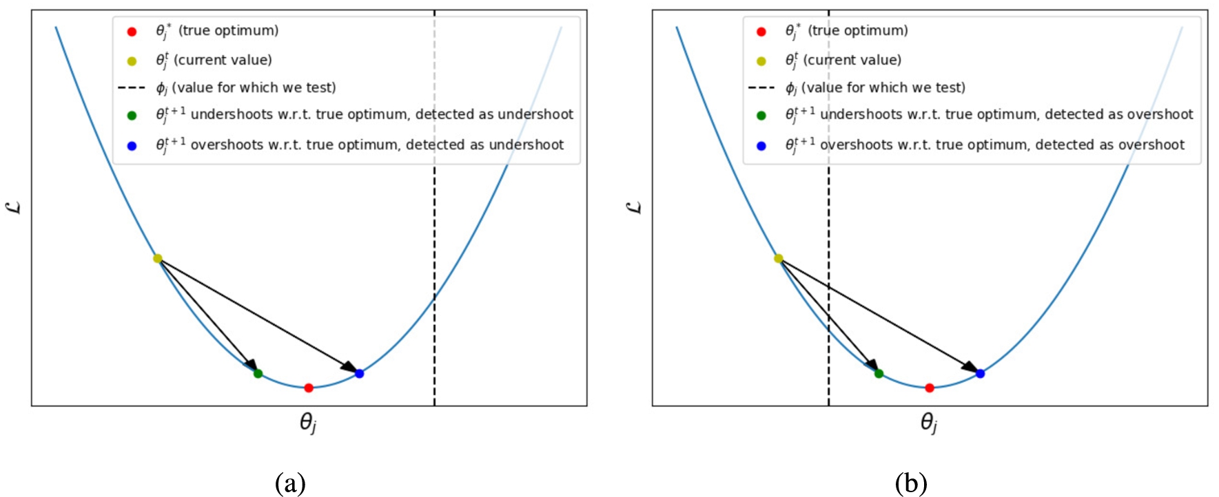
However, under-shooting can be problematic; for instance, a weight could be updated to a lower magnitude, while at the same time being far from 0. This can happen when a weight is approaching a non-zero local optimum, an occurrence which should not contribute towards a positive outcome of the aim test. By positive outcome, we refer to determining that $ϕ_{j} = 0$ is indeed a local optimum of $θ_{j}$ . A similar problem can occur for over-shooting, where a weight receives a large update that causes it to change its sign but not lie in the vicinity of 0. These scenarios, which we will refer to as deceitful shots going forward, are illustrated in the general case, where $ϕ_{j}$ can take any value, in Fig. 2(a) and Fig. 2(b). Following, we make two observations which help circumvent this problem.

Fig. 2.

In the plots above, the dotted vertical line represents the value at which the aim test is conducted, i.e. a value we would like to determine as a local optimum or not, while the red dot represents the value of a true local optimum. When testing for a value which is not a locally optimal value $ϕ_{j} \neq θ_{j}^{*}$ , over- or under-shooting around $ϕ_{j}$ can be merely a side-effect of that weight getting updated towards its true optimum $θ_{j}^{*}$ . These observations would then contribute towards the aim test returning a false positive outcome, I.e. $ϕ_{j} = θ_{j}^{*}$ . Whether we observe an over-shoot or an under-shoot in this case depends on the relationship between $ϕ_{j}$ and $θ_{j}^{*}$ . In (a), we have $ϕ_{j} > θ_{j}^{*}$ , where if the hypothesised and true optimum are sufficiently far apart, we observe an under-shoot. Conversely, in (b), we have $ϕ_{j} < θ_{j}^{*}$ and observe over-shooting.

Reducing the impact of deceitful shots. Firstly, one could reduce the impact of deceitful shots by also taking into account the distance of the weight to the hypothesised local optimum, i.e. $| θ_{j} - ϕ_{j} |$ , when conducting the aim test. In other words, the number of occurrences of under- and over-shooting should be weighed inversely proportional to this quantity, even if they would otherwise exceed κ.

Reducing the number of deceitful shots. Our second observation is that by ignoring updates which are not in the vicinity of $ϕ_{j}$ , the number of deceitful shots are reduced. In doing so, one could also simplify the aim test; with a sufficiently large perturbation to $θ_{j}$ , an update that might otherwise cause under-shooting can be made to cause over-shooting. Adding a perturbation of $\pm ϵ$ is, in effect, inducing a boundary around the tested value, $[ϕ_{j} - ϵ, ϕ_{j} + ϵ]$ ; all weights that get updated such that they fall into that boundary will be said to over-shoot around $ϕ_{j}$ . With this framework, checking for over-shooting is sufficient; updates that under-shoot and are within ϵ of the tested value are made to over-shoot (Fig. 3(a)) and updates which under-shoot but are not in the vicinity of $ϕ_{j}$ , i.e. a deceitful shot, are now not recorded at all (Fig. 3(b)). This can also be seen as restricting the aim test to only operate within a vicinity around $ϕ_{j}$ . Following, we piece together the ideas discussed so far in order to create a criterion for identifying and pruning weights that have locally optimal values at 0.

Fig. 3.

(a) All weights that under-shoot but are within ϵ of $ϕ_{j}$ will be made to over-shoot. (b) When testing at a value which is not a local optimum for $θ_{j}$ , i.e. $ϕ_{j} \neq θ_{j}^{*}$ , and adding a perturbation ϵ to $θ_{j}$ , not taking under-shooting into account means that if the weight gets updated such that it does not lie in the boundary around $ϕ_{j}$ induced by the perturbation, an event that would otherwise contribute to a false positive outcome for the aim test will not be recorded, so the likelihood of rejecting $ϕ_{j}$ as an optimum increases.

2.2. FlipOut: Applying the aim test for pruning

We present the two components necessary for applying the aim test for pruning. Specifically, in Section 2.2.1 we propose a saliency criterion that takes into account the number of times over-shooting has occurred as well as the distance of a weight from its hypothesised local optimum, as a result of the previously made observations in Section 2.1 regarding deceitful shots. Finally, in Section 2.2.2 we present a schema of adding perturbation into the weight tensor $θ$ .

2.2.1. Determining which weights to prune

Pruning weights that have local optima at or around 0 can obtain a high level of sparsity with minimal degradation in accuracy. The authors of [8] use the magnitude of the weights once the network is converged as a criterion; that is, the weights with the lowest absolute value, i.e. closest to 0, get pruned. The aim test can be used to detect whether a point represents a local optimum for a weight and can be applied before the network reaches convergence, during training. For pruning, one could then apply the aim test simultaneously for all weights with $ϕ = 0$ . We propose framing this as a saliency score; at time step t, the saliency $τ_{j}^{t}$ of a weight $θ_{j}^{t}$ is: $\begin{array}{l} (1a) & τ_{j}^{t} = \frac{| θ_{j}^{t} |^{p}}{{flips}_{j}^{t}} \\ (1b) & {flips}_{j}^{t} = \sum_{i = 0}^{t - 1} [sgn (θ_{j}^{i}) \neq sgn (θ_{j}^{i + 1})] \end{array}$ With perturbation added into the weight vector, it is enough to check for over-shooting, which is equivalent to counting the number of sign flips a weight has undergone during the training process when $ϕ_{j} = 0$ (Eq. (1b)); a scheme for adding such perturbation is described in Section 2.2.2. In Equation (1a), the numerator $| θ_{j}^{t} |^{p}$ represents the proximity of the weight to the hypothesised local optimum, $| θ_{j}^{t} - ϕ_{j} |^{p}$ (which is equivalent to the weight’s magnitude since we have $ϕ_{j} = 0$ for all weights). The hyperparameter p controls how much this quantity is weighted relative to the number of sign flips. When $p = 0$ , only the number of sign flips are taken into account, while when $p \to \infty$ , this criterion becomes equivalent to magnitude pruning.

When determining the amount of parameters to be pruned, we adopt the strategy from [6], i.e. pruning a percentage of the remaining weights each time, which allows us to target an exact level of sparsity. Given m, the number of times pruning is performed, r the percentage of remaining weights which are removed at each pruning step, k the total number of training steps, $d_{θ}$ the dimensionality of the weights and $‖ \cdot ‖_{0}$ the $L_{0}$ -norm, the resulting sparsity s of the weight tensor after training the network is simply: $\begin{matrix} (2) & s = 1 - \frac{‖ θ^{k} ‖_{0}}{d_{θ}} = {(1 - r)}^{m} \end{matrix}$ A desired final sparsity can then be determined by setting m and r appropriately. Moreover, for a specific level of sparsity, the combination of these two parameters is not unique and could be tweaked according to circumstances (i.e. one could choose to prune more frequently, but less parameters at a time, or vice-versa).

2.2.2. Perturbation through gradient noise

Adding gradient noise has been shown to be effective for optimization [32,44] in that it can help lower the training loss and reduce overfitting by encouraging an exploration in the parameter space, thus effectively acting as a regularizer. While the benefits of this method are helpful, our motivation for its usage stems from allowing the aim test to be performed in a simpler manner; weights that get updated closer to 0 will occasionally pass over the axis due to the injected noise, thus making checking for over-shooting sufficient.

We have seen in Section 2.1 that an update of SGD at time step t will cause a weight $θ_{j}^{t}$ to over-shoot around an optimum $θ_{j}^{*}$ if the inequality $η | g_{j}^{t} | < | θ_{j}^{t} - θ_{j}^{*} |$ holds. As such, methods that affect the magnitudes of the parameters or change the mechanics of the gradient computation can have an effect on the number of sign flips. Examples of these include weight decay, the $L_{1}$ regularizer, the choice of initialization strategy or using alternative optimization techniques such as momentum, Adam [18] or RMSprop [40]. This also holds true for the choice of learning rate, in that a large learning rate can cause a higher number of sign flips, and vice-versa. To make FlipOut more robust to methods that modify the magnitudes of the parameters, the variance of the noise distribution is scaled dynamically by the $L_{2}$ norm of the parameters of each layer $θ^{l}$ . We also normalize it by the number of weights and introduce a hyperparameter λ which acts as a multiplier. For a layer l and $d_{l}$ its dimensionality, the gradient for the weights in that layer used by SGD for updates is modified to: $\begin{array}{l} (3a) & {\hat{g}}^{t, l} \leftarrow g^{t, l} + λ ϵ^{t, l} \\ (3b) & ϵ^{t, l} \sim N (0, σ_{t, l}^{2}) \\ (3c) & σ_{t, l}^{2} = \frac{‖ θ^{t, l} ‖_{2}^{2}}{d_{l}} \end{array}$ As training is performed, it is desirable to reduce the amount of added noise so that the network can successfully converge. Previous works use annealing schedules by decaying the variance of the Gaussian distribution proportional to the current time step. Under our proposed formulation, however, explicitly using an annealing schema is not necessary. By pruning weights, the numerator in Eq. (3c) decreases, while the denominator remains constant. This ensures that annealing will be induced automatically through the pruning process, and there is no need for manually constructing a schedule.

Note that we have also experimented with other recipes for the variance of the Gaussian distribution (Eq. (3c)) which also fulfill the property of automatic annealing, such as the $L_{1}$ norm instead of $L_{2}$ or modifying the power of the numerator to 1 and normalizing it by $\sqrt{d_{l}}$ instead; its current form, however, has given us the best results overall.

Pruning periodically throughout training according to the saliency score in Eq. (1) in conjunction with adding gradient noise into the weights using Eq. (3) forms the FlipOut pruning method, which is summarised in Algorithm 1.

Algorithm 1

FlipOut

3. Related work

3.1. Deep-R

In Deep-R [2], the authors split the weights of the neural network into two matrices, the connection parameter $θ_{k}$ and a constant sign $s_{k}$ with $s_{k} \in {- 1, + 1}$ ; the final weights of the network are then defined as $θ ⊙ s$ . The connections whose $θ_{k}$ is negative are inactive; whenever a connection changes its sign, it is turned dormant and another randomly sampled connection is re-activated, ensuring the same sparsity level is maintained throughout training. Gaussian noise is also injected into the gradients during training.

Two similarities with our method can be observed here, namely the fact that the authors also use sign flipping as a signal for pruning a weight, and the addition of Gaussian noise. However, our methods differ in that we do not impose a set level of sparsity throughout training; instead, we use the number of sign flips of a weight in order to determine its saliency, while in Deep-R a single sign flip is required for a weight to be removed. Our method of injecting noise into the gradients also differs in that it does not explicitly encode an annealing scheme, allowing for the pruning process itself to reduce the noise throughout training.

3.2. Magnitude and uncertainty pruning

The M&U pruning criterion is proposed in [20]. Given a weight $θ_{j}$ , its uncertainty estimate ${\tilde{σ}}_{θ_{j}}$ and a parameter λ controlling the trade-off between magnitude and uncertainty, the M&U criterion will evaluate the saliency of the weight as: $\begin{matrix} τ_{j} = \frac{| θ_{j} |}{λ + {\tilde{σ}}_{θ_{j}}} \end{matrix}$ Uncertainty is estimated as the standard deviation across the previous n values of that weight, via a process called pseudo-bootstrapping. This criterion is a generalization of the Wald test, and is equivalent to it when $λ = 0$ .

Our method is similar in that our saliency score also normalizes the weight’s magnitude by a function of its past values. However, this method assumes asymptotic normality. While this is the case when using negative log-likelihood or an equivalent as the loss function, this property does not necessarily hold when using modified variants of the SGD estimator, such as Adam [18] or RMSprop [40]. In contrast, FlipOut is not derived from the Wald test and does not make any assumptions about the weight distribution at convergence.

3.3. Zeros, signs and the supermask

[46] conduct a series of ablation studies in order to determine why iterative magnitude pruning with rewinding, introduced by [6], works so well. Among others, they experiment with various rewinding strategies (i.e. the values that the kept weights are re-initialized to after a pruning step). They found that all tested strategies work better when the weights are reset such that their initial sign is kept, even when a single constant is used for all weights, i.e. at time step t a weight $θ_{j}^{t}$ is reset to $α \cdot sgn (θ_{j}^{0})$ . The authors conjecture that “optimizers work well anywhere in the correct sign quadrant for the weights, but encounter difficulty crossing the zero barrier between signs”.

While also emphasizing the importance of signs, we do not use it as a strategy for weight resetting. Instead, we consider a large number of sign flips during training as an indicator that a weight has a local optimum at 0, which makes it an ideal candidate for pruning, since it would then also be set at a point of optimality.

4. Experiments

We begin this section by detailing our experimental setup and the motivation behind it (Section 4.1). This is followed up by the method we have employed to determine favorable values for the hyperparameters p and λ of our proposed method (Section 4.2). Finally, we present our experiments: a comparison between FlipOut and baseline methods from literature (Section 4.3), an ablation study used to determine whether the performance of our method is simply a result of injecting gradient noise or if, indeed, the weights that have a local optimum at 0 can be reliably selected (Section 4.4), and a study into whether pruning and quantization can be used in conjunction and still maintain an acceptable level of performance (Section 4.5). All experiments have been implemented using the Pytorch deep learning library [34]. For reproducibility, we release our code at https://github.com/AndreiXYZ/flipout.

Table 1
Compression ratios, resulting sparsity levels and prune frequencies (in epochs) used in the experiments, assuming 350 epochs of training and that $50 %$ of the remaining weights are removed at each step

Compression ratio ( $\frac{d_{θ}}{‖ θ ‖_{0}}$ ) Resulting sparsity ( $1 - \frac{‖ θ ‖_{0}}{d_{θ}}$ ) Pruning frequency

$2^{2}$ 75% 117

$2^{4}$ 93.75% 70

$2^{6}$ 98.43% 50

$2^{8}$ 99.61% 39

$2^{10}$ 99.9% 32

Compression ratio ( $\frac{d_{θ}}{‖ θ ‖_{0}}$ )	Resulting sparsity ( $1 - \frac{‖ θ ‖_{0}}{d_{θ}}$ )	Pruning frequency
$2^{2}$	75%	117
$2^{4}$	93.75%	70
$2^{6}$	98.43%	50
$2^{8}$	99.61%	39
$2^{10}$	99.9%	32

4.1. General setup

4.1.1. Baselines

As baselines, we consider a slightly modified version of magnitude pruning [8] (Global magnitude), due to the similarity between its saliency criterion and that of our own method, SNIP [24] due to it being an easily applicable method which does not suffer from any of the issues that are commonly found in pruning methods (Section 1) and Hoyer-Square, as introduced in [45], for the state-of-the-art results that it has demonstrated. We also include random pruning (Random) as a control. For FlipOut, Global magnitude and Random, pruning is performed periodically throughout training. We compare these methods at five different compression ratios, chosen at regular log-intervals (Table 1); for Hoyer-square, the performance at those points is estimated by a sparsity-accuracy trade-off curve. Magnitude pruning, in its original formulation, performs pruning only once the network has reached convergence. However, employing this strategy can create a confounding variable: training time. Since we would like to compare all methods at equal training budgets, we have opted to simply perform pruning after a fixed number of epochs for these methods. Note that the training budget that we allocate allows all of the networks that we consider to reach convergence when trained without performing any pruning. We make an exception to this equal budget rule for Hoyer-Square, since it prunes after training and would otherwise not benefit from any SGD updates after sparsification. As such, we have performed an additional 150 epochs of fine-tuning without the regularizer, as per the original method, although we have found that the benefits of this are negligible and the accuracy drop incurred by pruning is relatively low as a consequence of the fact that the weight distribution was already peaked around 0. Following the strategy of [6], the magnitude pruning criterion proposed by [8] is modified to rank weights globally when a pruning decision is made, rather than in a layer-by-layer basis, so as to avoid creating bottleneck layers. For fairness, the same treatment is applied to all other methods that we test, including our own. Bias parameters have not been pruned since they only represent a small fraction of the total parameters in the networks that we test (Table 2). We also do not prune the learnable parameters in the batch normalization layers; an explanation for this is offered in Section 4.1.4. The levels of sparsities that we report going forward do not include the batch normalization and bias parameters.

The models that we test on are ResNet18 [11] and VGG19 [37] trained on the CIFAR-10 dataset [22], and DenseNet121 [15] trained on Imagenette [14]. An overview of the sizes of these models can be found in Table 2.

Table 2
The number of total parameters and biases for each model. The percentage of biases as compared to the total number of weights in the network is displayed in parenthesis. The last column represents the number of floating point operation required for a forward pass on a single sample, assuming an input size of $32 \times 32 \times 3$ for VGG19 and ResNet18, and $224 \times 224 \times 3$ for DenseNet121

Model Total params. Num. biases FLOPs

VGG19 20M 11k (0.0005%) 555M

ResNet18 11.1M 4.8k (0.0004%) 398M

DenseNet121 6.9M 41.8k (0.06%) 2.83B

Model	Total params.	Num. biases	FLOPs
VGG19	20M	11k (0.0005%)	555M
ResNet18	11.1M	4.8k (0.0004%)	398M
DenseNet121	6.9M	41.8k (0.06%)	2.83B

4.1.2. Hyperparameters

The training parameters for all experiments are taken from [41]; specifically, we use a learning rate of 0.1, batch size of 128, 350 epochs of training and a weight decay penalty of $5 e - 4$ . The learning rate is decayed by a factor of 10 at epochs 150 and 250. The networks are trained with the SGD optimizer with a momentum value of 0.9 [3]. For the methods that perform iterative pruning (Global magnitude, Random, FlipOut), we remove $50 %$ of the remaining weights at each pruning step, with the pruning frequencies chosen such that the compression ratios from Table 1 are achieved; we use the same pruning rates and frequencies across all three methods. SNIP accepts a single hyperparameter, namely the desired final sparsity, which we have chosen such that it matches the aforementioned compression ratios. For Hoyer-Square, which does not allow for a specific level of sparsity to be chosen and, instead, relies on parameter tuning, we generate a sparsity-accuracy trade-off curve by using 15 different values for the regularization term, ranging from $1 e - 7$ to $6 e - 3$ with 3 values at each decimal point, e.g. $1 e - 7$ , $3 e - 7$ , $6 e - 7$ , $1 e - 6$ etc., and a fixed pruning threshold of $1 e - 4$ . Finally, for FlipOut, we use the values of $p = 2$ (Eq. (1)) and $λ = 1$ (Eq. (3)) for all experiments, a choice we motivate in Section 4.2.

4.1.3. Metric

In order to motivate the choice of the metric used to compare between different pruning methods, we first revisit the practical benefits that can be achieved by pruning, namely the reduction of storage size, memory usage and computational speedup. The way in which these manifest in practice is dependent upon the pruning method used. For element-wise pruning (removing individual weights), a category in which our method and all tested baselines fall into, a dense weight matrix $θ$ can be converted to sparse representation using, for instance, the compressed sparse row (CSR) or compressed sparse column (CSC) formats [36]. Broadly speaking, these representations only store the indices of the nonzero elements, rather than the entire matrix, allowing for more efficient basic linear algebra subprogarms (BLAS) to be performed. As such, we employ as a metric the network’s test accuracy at the end of training at different levels of sparsity, averaged over multiple seeds; the RNG seeds used for these runs were kept consistent across methods. When comparing between different methods, the performance at equal sparsity levels is used. For Hoyer-Square, we estimate the performance at those points through its sparsity-accuracy trade-off curve. In literature, it is common practice to use the resulting compression ratio of the network as a proxy for measuring the gains in terms of size reduction and speedup [5,8,24,45]. While we also employ this methodology, we make two observations which showcase its caveats in the following.

Firstly, while there exists a strong correlation between sparsity and speedup, one could construct two neural networks of the same architecture with equal levels of sparsity, yet obtain different measurements in terms of inference time depending on how the active weights are distributed throughout the network. This is due to the fact that a weight in a filter from a convolutional layer gets reused multiple times when processing an input volume; as such, pruning a weight from a layer will reduce computation depending on the size of the volume used as input to that layer. In other words, pruning a weight from a layer that receives a larger input volume will generate a higher speedup.

Secondly, sparse networks have traditionally been unable to leverage compute kernels found in GPU accelerators due to the fact that memory reads are data-dependent and thus cannot fully utilize cache memory. This is pointed out by the authors of [29], which propose a more efficient sparse format and a recipe for pruning able to leverage Sparse Tensor Cores found in NVIDIA Ampere GPUs [33]. This format, however, only supports sparsity levels of up to $50 %$ (with a speedup of $2 \times$ ). While we believe that future research in this direction will be able to support higher sparsity levels, the current assumption that compression ratio reflects the level of speedup only holds when deploying sparse networks to CPUs, or when sparsity is up to $50 %$ on GPUs.

4.1.4. Batch normalization parameters should not be pruned

Batch normalization [16] is used in many neural network architectures in order to normalize the inputs to a layer, thus preserving gradient flow and allowing for more stable training. Given a mini-batch of m samples, and a layer activation $x^{k}$ , where each sample in the mini-batch generates one such activation, we have the collection $B = {x_{1 \dots m}^{k}}$ . For the k-th activation generated by the i-th sample from the mini-batch $x_{i}^{k}$ , the batch normalization algorithm first computes the empirical mean $μ_{B}^{k}$ and variance ${(σ_{B}^{k})}^{2}$ over the samples in the mini-batch for that activation. The output $y_{i}^{k}$ is then normalized using these values as follows: $\begin{matrix} {\hat{x}}_{i}^{k} \leftarrow \frac{x_{i}^{k} - μ_{B}^{k}}{\sqrt{{(σ_{B}^{k})}^{2} + ϵ}} \\ y_{i}^{k} \leftarrow γ^{k} {\hat{x}}_{i}^{k} + β^{k} \end{matrix}$ Here, ϵ is a small constant, added for numerical stability. The learnable parameters, $γ$ and $β$ are used to scale and shift the distribution once the inputs are normalized. Pruning these parameters can cause unintended consequences. For instance, let us consider the batch normalization output $y_{i}$ for a single training instance from a mini-batch. For a linear layer of n neurons, $y_{i}$ is a vector of size n; similarly, for a convolutional layer of n filters, $y_{i}$ will also be of size n. If we have $γ_{k} = 0$ , i.e. the k-th dimension of $γ$ has been pruned, we then have $y_{i}^{k} = β_{k}$ for all samples in the mini-batch, which can impede training. Moreover, if both $γ_{k}$ and $β_{k}$ are equal to 0, we have $y_{i}^{k} = 0$ . Since the input to the next layer is first passed through an activation function, for a function ζ with $ζ (0) = 0$ , such as the commonly used ReLU [31] or hyperbolic tangent functions, the next layer after batch normalization will receive 0 as input in the k-th position. This is equivalent to pruning all weights that contributed to generating that activation, i.e. all weights inbound to a neuron or the weights that form a filter, since they now no longer influence the network’s output, even though they are not set to 0 and still receive updates from backpropagation. In doing so, one could effectively prune more weights than intended, which can impact accuracy.

When comparing between different methods, this can affect the network’s performance in unforeseen ways, depending on the number of batch normalization parameters that get selected for pruning and even the particular dimensions of $β$ and $γ$ that get pruned. To allow for simpler comparisons, we have chosen not to prune the batch normalization parameters $β$ and $γ$ during our experiments for any of the methods tested.

4.2. Choosing the hyperparameters for FlipOut

We have experimented with different values of the two hyperparameters and found that $p = 2$ (Eq. (1a)) and $λ = 1$ (Eq. (3a)) offer optimal or near optimal results in all scenarios. In the following paragraphs, we detail the procedure used in determining these values.

4.2.1. Choosing λ

For λ, we have run all networks at 15 different values, ranging from 0.75 to 1.5 in increments of 0.05. The value of $p = 2$ was used. The networks are evaluated on a validation set, created by removing a random subset of samples from the training set. The size of the validation set was 10000 for CIFAR10 and 2000 for Imagenette. For our subsequent experiments, (Sections 4.3 and 4.4), the networks have been trained on the full training set. As a metric, we have used the accuracy of the networks at the end of training for the sparsity levels of $93.75 %$ and $99.9 %$ . We provide in Table 3 the accuracies generated by the optimal value of λ, as discovered through this process, and the ones generated at $λ = 1$ . Notice that the differences are almost negligible at $93.75 %$ sparsity. For the larger sparsity level the disparity increases, although the default value still remains within 2 percentage points of the optimum value for all networks considered. The largest gap can be seen for ResNet18 and DenseNet121, at approximately 1.7 and 1.5 percentage points, respectively. Since there are only two out of six cases in which optimizing λ has helped beyond a negligible amount, we have used the value of 1 for this hyperparameter throughout our experiments.

Table 3
Accuracies when using the best value of λ discovered by grid search and the value of $λ = 1$ at two levels of sparsity. The parantheses indicate the gain offered by the optimal parameter

Model Acc. at sparsity $93.75 %$ Acc. at sparsity $99.9 %$

$λ^{}$ $λ = 1$ $λ^{}$ $λ = 1$

ResNet18 94.58 (+0.02) 94.56 83.75 (+1.68) 82.07

VGG19 93.07 (+0.11) 92.96 87.72 (+0.48) 87.24

DenseNet121 89.75 (+0.0) 89.75 73.5 (+1.45) 72.05

Model	Acc. at sparsity $93.75 %$	Acc. at sparsity $99.9 %$
ResNet18	94.58 (+0.02)	94.56	83.75 (+1.68)	82.07
VGG19	93.07 (+0.11)	92.96	87.72 (+0.48)	87.24
DenseNet121	89.75 (+0.0)	89.75	73.5 (+1.45)	72.05

4.2.2. Choosing p

We perform similar experiments for p on five values, $p \in {0, \frac{1}{2}, 1, 2, 4}$ and λ set to 1. Note that the value of $p = 0$ corresponds to the case when the magnitudes of the weights are not taken into account; that is, the pruning decisions will be made solely based on the number of sign flips. As can be seen in Table 4, the value of $p = 2$ consistently outperforms all other tested values, with the exception of ResNet18 at $99.9 %$ sparsity, for which the value of $p = 4$ achieves better results by approximately 1 percentage point. Another interesting observation is that the values of 1, 2 and 4 tend to perform better than 0 and $\frac{1}{2}$ ; we conjecture that this is due to the fact that deceitful shots (Section 2.1) occur when not taking into account the distance between the weight and its hypothesised local optimum, which have a negative impact on the pruning decision. This can be especially observed at the higher sparsity level and in the case of DenseNet121, where pruning with $p = 0$ causes the network to not perform better than random guessing. Given that the value of $p = 2$ is favored in 5 out of 6 cases, we have decided to use it as a default value in our subsequent experiments.

Table 4
Table of results for different values of p at two levels of sparsity

Model Acc. at sparsity $93.75 %$ Acc. at sparsity $99.9 %$

$p = 0$ $p = \frac{1}{2}$ $p = 1$ $p = 2$ $p = 4$ $p = 0$ $p = \frac{1}{2}$ $p = 1$ $p = 2$ $p = 4$

ResNet18 93.71 88.39 94.18 94.26 94.11 72.69 77.08 79.83 82.07 83.15

VGG19 91.68 82.44 92.56 92.96 92.57 81.48 80.69 86.01 87.24 86.64

DenseNet121 10.35 77.40 88.9 89.75 88.86 10.35 10.35 70.85 72.05 60.55

Model	Acc. at sparsity $93.75 %$	Acc. at sparsity $99.9 %$
ResNet18	93.71	88.39	94.18	94.26	94.11	72.69	77.08	79.83	82.07	83.15
VGG19	91.68	82.44	92.56	92.96	92.57	81.48	80.69	86.01	87.24	86.64
DenseNet121	10.35	77.40	88.9	89.75	88.86	10.35	10.35	70.85	72.05	60.55

Fig. 4.

Results of our pruning experiments on the 3 reference networks. Each point is averaged over 3 runs; error bars indicate standard deviation. (a) ResNet18 on CIFAR 10. (b) VGG19 on CIFAR10. (c) DenseNet121 on ImageNette.

4.3. Comparison to baselines

The results for the three models tested are found in Fig. 4. FlipOut obtains state-of-the-art performance on ResNet18 and VGG19 for sparsity levels of $99.61 %$ and beyond. For the highest tested sparsity level, it outperforms the second-best method by 1.9 and 4.5 percentage points, respectively (Fig. 4(a), 4b). Notably, when using FlipOut on VGG19 for this sparsity, the drop in accuracy compared to the unpruned model is only 6.2 percentage points. At the same time, it remains competitive with other baselines for lower degrees of sparsity, staying within a 1 percentage point difference compared to the best method and with a minimal drop relative to the unpruned model. For DenseNet121, however, Hoyer-Square dominates all other methods tested in most cases (Fig. 4(c)), with FlipOut as second best for the highest sparsity level.

Interestingly, the simple criterion of magnitude pruning, when modified to rank the weights globally instead of a layer-by-layer basis, is competitive with other, more recent, baselines, and even obtains state-of-the-art results for moderate levels of sparsity. However, at high levels of sparsity, which correspond to more frequent and implicitly earlier pruning steps (Table 1) there is a performance degradation. This suggests that the magnitude of a weight by itself is not a good measure of saliency when the network is far from reaching convergence. It is also worth noting that SNIP collapses at high levels of sparsity, causing the network to perform no better than random guessing. Upon inspecting these cases (not shown for visibility) we noticed that at least one layer has been entirely pruned, effectively blocking any signal from passing. Interestingly, this does not happen for any of the other baselines (except for Random). We conjecture that this collapse as well as the cases where SNIP performs worse than random pruning (Fig. 4(b)) are a result of pruning at initialization; pruning too early can cause the saliency criterion to be inaccurate, but also impedes training in and of itself.

During our experiments, we empirically observed that Hoyer-Square requires extensive hyperparameter tuning for optimal performance. Our method, however, has strong default values and can also target the final sparsity directly, while also not requiring additional epochs of fine-tuning. Finally, SNIP, the only other baseline which does not suffer from any of the issues commonly found among pruning methods (Section 1) compromises on performance for high levels of sparsity, whereas FlipOut does not.

Fig. 5.

Results of the ablation study on the noise. Global magnitude without noise addition is also shown for comparison. (a) ResNet18 on CIFAR 10. (b) VGG19 on CIFAR10. (c) DenseNet121 on ImageNette.

4.4. Is it just the noise?

The performance of FlipOut could simply be a result of the noise addition, which is known to aid optimization [32,44]. To investigate this, we perform experiments with global magnitude as the pruning criterion in which we add noise into the gradients using the recipe from Equation (3c) and compare it to our own method. Notably, the saliency criterion of these two methods differ only in that FlipOut normalizes the magnitude by the number of sign flips (denominator in Eq. (1a)). The hyperparameters were kept at their default values of $p = 2$ for FlipOut and $λ = 1$ for both methods. We also include runs of FlipOut where no noise was added, i.e. $λ = 0$ . These serve as a control, decoupling the two novel components of our method: noise addition and scaling magnitudes by the number of sign flips. The same pruning rates and frequency of pruning steps have been used as before (Table 1). The results are illustrated in Fig. 5.

For sparsity levels up to $98.44 %$ , adding gradient noise causes a slight deterioration on performance, as can be seen by the fact that both global magnitude and FlipOut with $λ = 0$ outperform their noisy counterparts. It can also be seen that FlipOut with $λ = 1$ performs comparably to noisy global magnitude, indicating that measuring saliency by sign flips does not benefit accuracy in these regimes compared to using only the magnitude, and the performance gap between the noisy and non-noisy methods is likely a result of noise addition. For sparsity levels of $99.61 %$ and above, however, the opposite is true. It seems that gradient noise disproportionately benefits networks with a small number of remaining parameters; we conjecture that this is due to the fact that the exploration in parameter space induced by noise is more effective when that space is heavily constrained. Focusing on the highest level of sparsity, FlipOut outperforms noisy global magnitude on VGG19 (Fig. 5(b)) and DenseNet121 (Fig. 5(c)) by 1.2 and 8.2 percentage points, respectively, while being outperformed by 0.8 percentage points on ResNet18 (Fig. 5(a)). The standard deviation of FlipOut at this point is lower than for noisy global magnitude for all networks tested, making it more robust to initial conditions and the noise sampling process. At this level, the addition of gradient noise to FlipOut also shows performance boosts compared to its non-noisy counterpart, namely 9.3 percentage points for ResNet18, 3.2 for VGG19 and 3.7 for DenseNet121. The benefits caused by adding noise to global magnitude as compared to adding it to FlipOut are similar for VGG19; however, it is relatively small for ResNet18 at 2.6 percentage points and even causes a 2 percentage point drop in performance for DenseNet121.

Since FlipOut with $λ = 1$ outperforms noisy global magnitude in 2 out of 3 cases for the highest level of sparsity while maintaining similar performance in all other cases as well as being less sensitive to the choice of seed, we conclude that its results cannot be explained only by the addition of noise and is also caused by the sign flips being taken into account when computing saliency.

Additionally, we conjecture that occurrences of under-shooting are indeed converted into over-shooting when adding gradient noise, allowing FlipOut to more accurately compute saliencies. This is evidenced by the fact that gradient noise addition benefits FlipOut more so than it does global magnitude, and implies that our method of dealing with deceitful shots is sound.

4.5. Combining pruning and quantization

We study whether quantization can be successfully applied in conjunction with pruning. Through quantization, we refer to the practice of converting a neural network’s weights and activations to 8 bits (whereas typical applications use 32). This technique has the same practical advantages as pruning, namely a reduced memory footprint and model storage size as well as computational speedup (in this case by a factor of up to $4 \times$ ).

We begin by motivating our choice of quantization scheme in Section 4.5.1 and detail our experimental setup in Section 4.5.2. Finally, we analyze our results in Section 4.5.3.

4.5.1. Sparsity preserving quantization

According to the authors of [21], a variable x of range $(x_{\min}, x_{\max})$ stored as a floating point in 32 bits of precision can be quantized to an 8 bit integer as follows: $\begin{array}{l} x_{int} = ⌊ \frac{x}{Δ} ⌉ + z \\ x_{Q} = clamp (x_{int}, [0, 255]) \end{array}$ where Δ and z are known as scale and zero-point, respectively, the round function $⌊ \cdot ⌉$ returns the integer nearest to the input value provided and $clamp (\cdot, [\cdot, \cdot])$ returns the nearest interval bound if the provided value lies outside of it and performs the identity function otherwise. Here, due to common neural network operations (such as padding) it is desirable to quantize 0 without error; as such, the zero-point z is restricted to be an integer. This general scheme is known as uniform affine quantization. Note that this must be applied to both the weights and activations in order for the computation of the forward pass to be carried out fully in 8 bits.

However, applying this scheme to a sparse network has negative consequences. All previously pruned weights of value $x = 0$ will become $x_{int} = z$ . For any value of $z \neq 0$ , this has the effect of undoing the sparsity generated by pruning. As such, we employ in our experiments a strategy similar to that of [10]. Namely, for weights, we use the symmetric quantization scheme, which restricts z to be 0, and use signed integers as the interval to map to, i.e. $[- 128, 127]$ . The weight quantization scheme then becomes: $\begin{array}{l} x_{int} = ⌊ \frac{x}{Δ} ⌉ \\ x_{Q} = clamp (x_{int}, [- 128, 127]) \end{array}$

For the activations, there is no need to preserve sparsity. As such, we employ the symmetric quantization scheme with signed integers. The scale and zero-point can then be derived depending on the observed minimum and maximum values $x_{\min}$ , $x_{\max}$ for every tensor as follows [35]: $\begin{array}{l} Weights: s = \frac{2 max (| x_{\min} |, x_{\max})}{255} z = 0 \\ Activations: s = \frac{(x_{\max} - x_{\min})}{255} z = - ⌊ \frac{x_{\min}}{s} ⌉ \end{array}$

4.5.2. Setup

We first train and prune ResNet18 and VGG19 as per the methodology described in Section 4.1.1 and the same hyperparameters as in Section 4.1.2. As pruning methods, we have tested FlipOut and compared it to Global Magnitude as the baseline, due to the similarity of their saliency criteria. Following this step, we perform post-training quantization, where we calibrate the model on the training set in order to determine the interval bounds $x_{\min}$ , $x_{\max}$ for each tensor. We have tested five such different methods which vary in terms of granularity and in how the bounds are computed. Specifically, we have experimented with using the boundaries observed during calibration for each layer (MinMax), for each individual channel (PC-MinMax), a moving average of the boundaries for each layer (MA-MinMax) and for each channel (MA-PC-MinMax) as well as a histogram method (Histogram). The Histogram method bins the observed values, keeping in memory the values as well as the boundaries for each bin. These bins are updated continuously as calibration is performed. Following calibration, a nonlinear search over the bin boundaries is performed such that the quantization error with respect to the full-precision model is minimized [35]. In effect, this method will remove outlier values observed during calibration.

For hyperparameters, we use an averaging constant of 0.01 for the moving average methods and 2048 as the number of bins for the histogram method. Note that MinMax and PC-MinMax do not have any hyperparameters. For calibration, we use the same random seed that was used to generate the trained-and-pruned netoworks and a batch size of 128 in all cases; the random seeds involved in this set of experiments are different than those from Section 4.3 and 4.4. While we have also experimented with using a varying number of epochs for the calibration times, we have found that a single epoch is sufficient and further calibration does not yield any significant improvements. We compare both models (VGG19 and ResNet18) across different levels of sparsity using the five aforementioned calibration schemas. For reference, we also include baseline results, where we simply train the networks without any pruning and apply post-training quantization. As before, 3 runs with different random seeds are used to generate each result. We have also attempted to run these experiments on the DenseNet121 network; however, the results have been unstable, with high degrees of variance and performance losses which would render the network’s predictions unusable in a practical scenario. As such, we defer these experiments to future work, where other quantization methods, such as [17], might be tested.

Fig. 6.

Table of results for VGG19 when pruning is applied, using either FlipOut or Global Magnitude, with five different quantization schemes applied post-training. Baseline results when only quantization is applied are also included. Each bar chart represents an average over 3 runs using different random seeds.

Fig. 7.

Table of results for ResNet18 when pruning is applied, using either FlipOut or Global Magnitude, with five different quantization schemes applied post-training. Baseline results when only quantization is applied are also included. Each bar chart represents an average over 3 runs using different random seeds.

4.5.3. Results

We present our results for VGG19 and ResNet18 in Figs 6 and 7, respectively. Notably, it can be seen that the moving average methods obtain equal results to their regular counterparts for all cases we have tested. This suggests that the averaging constant of 0.01 is not large enough to modify the computed bounds with the number of calibration steps that we have used. The behavior of the Histogram method, however, is drastically different depending on the type of network that it is applied to. For VGG19 it has the worst performance of the five when no pruning is performed, while for ResNet18 it is the best in some scenarios, albeit not by a wide margin. A similar pattern can be seen when we apply it to pruned networks, although an additional failure mode appears at the highest pruning frequency for ResNet18 where its relative drop in accuracy is higher than for the other calibration schemes. For VGG19, its performance drop is at levels where it would be considered unacceptable; at the highest level of sparsity for global magnitude it even degenerates to the random prediction case. Overall, the best performing calibration method is MinMax; in the case of VGG19 this is true by a wide margin, while for ResNet18 there are two exception cases where Histogram performs slightly better, namely for FlipOut at a prune frequency of 70 and Global Magnitude at a frequency of 39. Since in a majority of cases the MinMax scheme attains superior performance, all of our comparisons going forward will refer strictly to it.

Comparing the results of pruning and quantization to the baseline case of just quantization, the drop in accuracy for the first 3 levels of sparsity is contained at approximately $1 %$ for both VGG19 and ResNet18, irrespective of the pruning method used, in the case of the MinMax calibration scheme. For the fourth level of sparsity, however, the gap increases, at approximately $2.5 %$ and $3.8 %$ for VGG19 and ResNet18, respectively. At the final sparsity level, this degradation exceeds $8 %$ and $14 %$ for the two networks.

A comparison can also be drawn between the two compression methods, pruning and quantization, when applied in isolation; a sparsity of $75 %$ is equivalent to storing the weights of the network on a bitwidth that is 4 times as small in terms of total bits of information in the network (disregarding bias and batch normalization parameters). The quantization results for VGG19 and ResNet18 when applying the MinMax scheme and no pruning are $90.18 %$ and $94.24 %$ , respectively. When pruning, using a frequency of 117 (Table 1), the drop in accuracy in relatively negligible, while quantization degrades performance by approximately $2.7 %$ and $0.4 %$ , respecitely. We highlight these findings in Table 5, with additional results for when both methods are applied. Note that applying quantization on an already pruned network is equivalent to increasing the compression ratio by $4 \times$ . As such, a network of $75 %$ sparsity when quantized will have the same number of bits of information stored in its weights as a network of $93.75 %$ sparsity (a pruning frequency of 50 in our experiments). It can be seen that for VGG19, only applying pruning is preferable to quantization. This holds true even when the level of sparsity is increased and we compare that to lower sparsity and quantization. For this model, it seems that quantization is responsible for most of the performance gap. Interestingly, however, for ResNet18, while pruning with $75 %$ sparsity is still preferable to quantization, the joint strategy yields better performance when compared to the equivalent compression ratio obtained by just pruning. These results hold for both pruning criteria that we have tested and the difference in accuracies between them are neglibile at these sparsities; as such, we cannot conclude that either of the two pruning methods generates a network that is more amenable to quantization.

Table 5
Table of results for independently pruned, quantized (using the MinMax calibration scheme), jointly pruned and quantized as well as full models, averaged over 3 seeds. Numbers are expressed as accuracy percentages

Model Full Quant. Pruned $75 %$ Pruned $75 %$ + Quant. Pruned $93.75 %$

FlipOut Magnitude FlipOut Magnitude FlipOut Magnitude

VGG19 92.86 90.18 92.81 92.84 90.17 90.6 92.59 92.43

ResNet18 94.65 94.24 94.6 94.53 94.21 94.05 93.63 93.69

Model	Full	Quant.	Pruned $75 %$	Pruned $75 %$ + Quant.	Pruned $93.75 %$
VGG19	92.86	90.18	92.81	92.84	90.17	90.6	92.59	92.43
ResNet18	94.65	94.24	94.6	94.53	94.21	94.05	93.63	93.69

5. Discussion

In this work, we introduce the aim test, a general method for determining whether a point represents a local optimum for a weight. We then show how the impact of observations that lead to a false positive outcome of the aim test (deceitful shots) can be minimized by taking into consideration the distance of the weight from the value tested as a local optimum and by adding gradient noise while ignoring the occurrences of under-shooting entirely. In order to simultaneously prune and set weights to points of local optima, one could then simply conduct the aim test at $ϕ_{j} = 0$ for all weights simultaneously and cast it as a saliency criterion, whereby the weights with the lowest score are removed.

This method, coined FlipOut, demonstrates several desirable properties. Firstly, it is computationally tractable, as it only involves the magnitudes of the weights and a count over the number of sign flips, which scales linearly with the dimensionality of $θ$ . Additionally, the desired level of sparsity can be directly selected by setting the pruning rate and pruning frequency appropriately (Eq. (2)). Finally, since the aim test can be applied before convergence, pruning with FlipOut only requires a single training run.

We perform experiments on a variety of commonly used computer vision architectures and demonstrate that there exist values for the hyperparameters p and λ (Eq. (1a), Eq. (3a)) which generate near optimal results in the majority of cases, eliminating the need for extensive hyperparameter search. Moreover, we show that FlipOut has similar performance to other baseline methods from literature, and even achieves state-of-the-art results at the highest levels of sparsity for 2 out of 3 of the tested networks. We also conduct ablation tests in order to determine the cause of its performance. We find that the addition of gradient noise plays an important role in our method, particularly in high sparsity regimes, but cannot by itself explain the performance of FlipOut. This implies that the other component of our algorithm, scaling the magnitude by the number of sign flips in the computation of the saliency score, is also a significant factor. Finally, in Section 4.5 we study whether pruning can be applied conjointly with quantization, a technique which promises the same practical advantages. While we find little difference between using FlipOut and Global Magnitude as the pruning criteria, combining these two methods is feasible in terms of the resulting accuracy of the network when moderate levels of sparsity (up to $98.43 %$ ) are used for VGG19 and ResNet18, despite the fact that a restrictive quantization schema needs to be used in order to preserve sparsity, which may be suboptimal in certain scenarios.

As a recommendation for practitioners, the choice of compression techniques used should depend on the target platform to which neural networks are deployed and the desired level of acceleration. With current generation GPU accelerators, one can expect a maximum speedup factor in inferencing of $2 \times$ when using an unstructured pruning algorithm, corresponding to a sparsity level of $50 %$ . As such, for this use case, we recommend using FlipOut with a pruning rate and frequency set such that this level of sparsity is achieved. While our experiments only use sparsity levels of $75 %$ and up, we have noticed that regardless of the pruning method used, the degradation in performance is highly correlated to the degree of sparsity in the network; since little to no accuracy drop was observed at $75 %$ sparsity when using FlipOut, we expect this to also hold for a less sparse network (i.e. at $50 %$ ). Succesfully leveraging graphics accelerators beyond this level of speedup, however, requires either using quantization in isolation or combining the two methods. From our experiments in Section 4.5.3, we have observed low performance losses when using $75 %$ sparsity and the MinMax quantization scheme; as such, we recommend this combination of techniques when acceleration of up to $8 \times$ is required. While not covered in our own experiments, earlier works have shown that symmetric post-training quantization schemes, when used in isolation, can maintain the network performance almost intact [21], and as such constitute an attractive option when a speedup of up to $4 \times$ is desirable. With previous generation graphics accelerators, unstructured sparsity is not supported and one would have to resort to using structured pruning methods [12,25] and/or quantization.

When deployment is targeted to CPUs, on the other hand, no such restrictions exist and any method could be applied. In this case, both pruning with FlipOut and quantization could be applied separately for a speedup of $4 \times$ ; specifically, symmetric quantization is preferred, as per the results in [21]. For higher levels of speedup, however, using FlipOut with a higher level of sparsity is preferrable to using pruning and asymmetric quantization (necessary in order to preserve the sparsity created by pruning). This is supported by our resutls from Table 5, which illustrate that the performance loss when combining these two methods is mostly a result of quantization.

6. Limitations & future work

In this section, we address the shortcomings of our research and discuss potential avenues for future work.

Firstly, we have only conducted tests for convolutional neural networks for the task of object classification. As such, it would be interesting to study whether FlipOut is effective when using architectures that handle sequential data [13,42] or even generative models [7,19]. Moreover, we have used a limited sample size in order to keep our experiments feasible (Sections 4.1.1 and 4.5.3), which means that we could not run statistical significance tests, although our experiments did allow for some degree of informed speculation. Repeating the experiments with a larger sample size could then help to validate our claims in a more principled manner. Also, for the quantization-only experiments from Section 4.5.3 we have used the sparsity preserving schema described in Section 4.5.1. However, when quantization is applied in isolation, there is no need to restrict the zero-point to 0 and use a signed integer interval. Particularly, it has been documented in [21] that for certain networks an asymmetric schema (i.e. the zero-point can take arbitrary values) is preferable. It is therefore possible that the results presented in Table 5 for isolated quantization could be improved by applying a different schema.

At the same time, we believe our method can inspire novel research directions. For instance, FlipOut in its current form performs element-wise pruning and, as such, requires converting the weight matrix $θ$ to a sparse format in order to yield speedup and compression. A two-to-four sparsity pattern (two weights at every block of four are pruned), able to leverage sparse tensor cores present in current generation graphics accelerators, is described in [29]. Our proposed method, while able to achieve high degrees of sparsity, does not guarantee that this pattern is preserved. As such, possible lines of research might include specifically enforcing a two-to-four sparsity pattern at the algorithm level or extending FlipOut to perform structural pruning (where speedup and compression can be achieved directly). Regarding our experiments in using pruning jointly with quantization, we have noticed that for certain scenarios, a large part of the performance degradation is caused specifically by quantization, likely due to the restrictive schema required to preserve the sparsity obtained through pruning (described in Section 4.5.1). Quantization-aware training [17] has been shown to generally outperform post-training quantization [21], with the caveat that it cannot be directly applied to an already trained network. Therefore, a set of experiments where quantization-aware training is employed in conjunction with our pruning method, a strategy akin to that of [10], could reveal whether the gap between the dense 32-bits models and the sparse 8-bits ones could be further closed, notably for the DenseNet121 architecture, where our current setup has yielded high instability.

Moreover, our work has potential applications in optimization; the issue of pathological curvature [28] is known to hinder the generalization ability of neural networks and has been traditionally dealt with by using optimization techniques that dampen oscillations across SGD updates [18,40]. The aim test could also serve as one such solution, whereby weights are set to a value they oscillate around, potentially aiding optimization.

Finally, it is our hope that this work can inspire other researchers to develop novel pruning and/or quantization methods of their own. Since a high degree of correlation has been established between computational power and performance of deep learning systems [39], an ever increasing computational demand is to be expected. It is, therefore, not unlikely that model compression techniques will become an ubiquitous component of deep learning pipelines. Methods that are easily applicable and add little additional time cost on the practitioner’s part can help in their widespread adoption.

Footnotes

Acknowledgements

We would like to thank BrainCreators B.V. for the funding of this research. We would also like to thank the University of Amsterdam for the provided guidance and counsel.

References

A.C.

Apostol,

M.C.

Stol and

Forré, FlipOut: Uncovering redundant weights via sign flipping, in: Artificial Intelligence and Machine Learning,

Baratchi,

Cao,

W.A.

Kosters,

Lijffijt,

J.N.

van Rijn and

F.W.

Takes, eds, Springer International Publishing, Cham, 2021, pp. 15–29. ISBN 978-3-030-76640-5. doi:10.1007/978-3-030-76640-5_2.

Bellec,

Kappel,

Maass and

Legenstein, Deep rewiring: Training very sparse deep networks, in: International Conference on Learning Representations, 2018.

Bottou, Online algorithms and stochastic approximations, in: Online Learning and Neural Networks, Cambridge University Press, Cambridge, UK, 1998, revised, Oct. 2012.

Brock,

Donahue and

Simonyan, Large scale GAN training for high fidelity natural image synthesis, in: International Conference on Learning Representations, 2019.

Ding,

Zhou,

Guo,

Han,

Liu et al., Global sparse momentum sgd for pruning very deep neural networks, in: Advances in Neural Information Processing Systems, 2019.

Frankle and

Carbin, The lottery ticket hypothesis: Finding sparse, trainable neural networks, in: International Conference on Learning Representations, 2019.

Goodfellow,

Pouget-Abadie,

Mirza,

Xu,

Warde-Farley,

Ozair,

Courville and

Bengio, Generative adversarial nets, in: Advances in Neural Information Processing Systems, 2014, pp. 2672–2680.

Han,

Pool,

Tran and

Dally, Learning both weights and connections for efficient neural network, in: Advances in Neural Information Processing Systems, 2015.

Hassibi and

D.G.

Stork, Second order derivatives for network pruning: Optimal brain surgeon, in: Advances in Neural Information Processing Systems, 1993.

10.

Hawks,

Duarte,

N.J.

Fraser,

Pappalardo,

Tran and

Umuroglu, Ps and Qs: Quantization-aware pruning for efficient low latency neural network inference, arXiv preprint (2021). arXiv:2102.11289.

11.

He,

Zhang,

Ren and

Sun, Deep residual learning for image recognition, in: 2016 IEEE Conference on Computer Vision and Pattern Recognition (CVPR), 2016. doi:10.1109/CVPR.2016.90.

12.

He,

Zhang and

Sun, Channel pruning for accelerating very deep neural networks, in: Proceedings of the IEEE International Conference on Computer Vision, 2017, pp. 1389–1397.

13.

Hochreiter and

Schmidhuber, Long short-term memory, Neural Computation 9(8) (1997), 1735–1780. doi:10.1162/neco.1997.9.8.1735.

14.

Howard, Imagenette, 2019, Accessed April 6th, 2020 at https://github.com/fastai/imagenette.

15.

Huang,

Liu,

Van Der Maaten and

K.Q.

Weinberger, Densely connected convolutional networks, in: 2017 IEEE Conference on Computer Vision and Pattern Recognition (CVPR), 2017. doi:10.1109/CVPR.2017.243.

16.

Ioffe and

Szegedy, Batch normalization: Accelerating deep network training by reducing internal covariate shift, in: Proceedings of the 32nd International Conference on Machine Learning, Vol. 37, ICML’15, JMLR.org, 2015.

17.

Jacob,

Kligys,

Chen,

Zhu,

Tang,

Howard,

Adam and

Kalenichenko, Quantization and training of neural networks for efficient integer-arithmetic-only inference, in: Proceedings of the IEEE Conference on Computer Vision and Pattern Recognition, 2018, pp. 2704–2713.

18.

Kingma and

Ba, Adam: A method for stochastic optimization, in: International Conference on Learning Representations, 2015.

19.

D.P.

Kingma and

Welling, Auto-encoding variational Bayes, in: Proceedings of the 2nd International Conference on Learning Representations, 2014.

20.

Ko,

Oehmcke and

Gieseke, Magnitude and uncertainty pruning criterion for neural networks, in: 2019 IEEE International Conference on Big Data (Big Data), 2019. doi:10.1109/BigData47090.2019.9005692.

21.

Krishnamoorthi, Quantizing deep convolutional networks for efficient inference: A whitepaper, arXiv preprint (2018). arXiv:1806.08342.

22.

Krizhevsky, Learning multiple layers of features from tiny images, 2009.

23.

LeCun,

J.S.

Denker and

S.A.

Solla, Optimal brain damage, in: Advances in Neural Information Processing Systems, Vol. 2, 1990.

24.

Lee,

Ajanthan and

Torr, SNIP: Single-shot network pruning based on connection sensitivity, in: International Conference on Learning Representations, 2019.

25.

Li,

Kadav,

Durdanovic,

Samet and

H.P.

Graf, Pruning filters for efficient ConvNets, in: International Conference on Learning Representations, 2017.

26.

Liu,

Xu,

Shi,

R.C.C.

Cheung and

H.K.H.

So, Dynamic sparse training: Find efficient sparse network from scratch with trainable masked layers, in: International Conference on Learning Representations, 2020.

27.

Louizos,

Welling and

D.P.

Kingma, Learning sparse neural networks through

L_{0}

regularization, in: International Conference on Learning Representations, 2018.

28.

Martens, Deep learning via Hessian-free optimization, in: ICML, Vol. 27, 2010, pp. 735–742.

29.

Mishra,

J.A.

Latorre,

Pool,

Stosic,

Venkatesh,

Yu and

Micikevicius, Accelerating sparse deep neural networks, arXiv preprint (2021). arXiv:2104.08378.

30.

Molchanov,

Ashukha and

Vetrov, Variational dropout sparsifies deep neural networks, in: International Conference on Machine Learning, 2017.

31.

Nair and

G.E.

Hinton, Rectified linear units improve restricted Boltzmann machines, in: Proceedings of the 27th International Conference on Machine Learning (ICML-10), 2010.

32.

Neelakantan,

Vilnis,

Q.V.

Le,

Sutskever,

Kaiser,

Kurach and

Martens, Adding gradient noise improves learning for very deep networks, arXiv e-prints (2015).

33.

NVIDIA A100 tensor core GPU architecture. https://images.nvidia.com/aem-dam/en-zz/Solutions/data-center/nvidia-ampere-architecture-whitepaper.pdf.

34.

Paszke,

Gross,

Massa,

Lerer,

Bradbury,

Chanan,

Killeen,

Lin,

Gimelshein,

Antiga,

Desmaison,

Kopf,

Yang,

DeVito,

Raison,

Tejani,

Chilamkurthy,

Steiner,

Fang,

Bai and

Chintala, PyTorch: An imperative style, high-performance deep learning library, in: Advances in Neural Information Processing Systems, Vol. 32, Curran Associates, Inc., 2019. http://papers.neurips.cc/paper/9015-pytorch-an-imperative-style-high-performance-deep-learning-library.pdf .

35.

Pytorch quantization official documentation. https://pytorch.org/docs/stable/torch.quantization.html.

36.

Saad, Iterative Methods for Sparse Linear Systems, SIAM, 2003.

37.

Simonyan and

Zisserman, Very deep convolutional networks for large-scale image recognition, in: International Conference on Learning Representations, 2015.

38.

Strubell,

Ganesh and

McCallum, Energy and policy considerations for deep learning in NLP, in: Proceedings of the 57th Annual Meeting of the Association for Computational Linguistics, 2019. doi:10.18653/v1/P19-1355.

39.

N.C.

Thompson,

Greenewald,

Lee and

G.F.

Manso, The computational limits of deep learning, arXiv preprint (2020) arXiv:2007.05558.

40.

Tieleman and

Hinton, Lecture 6.5—rmsprop: Divide the gradient by a running average of its recent magnitude, 2012.

41.

Train CIFAR10 with PyTorch (GitHub Repository), Unknown Author, PyTorch CIFAR-10 GitHub Repository, 2017, Accessed April 6th, 2020 at https://github.com/kuangliu/pytorch-cifar/.

42.

Vaswani,

Shazeer,

Parmar,

Uszkoreit,

Jones,

A.N.

Gomez,

Ł.

Kaiser and

Polosukhin, Attention is all you need, in: Advances in Neural Information Processing Systems, 2017.

43.

Verdenius,

Stol and

Forré, Pruning via iterative ranking of sensitivity statistics, arXiv e-prints (2020). arXiv:2006.00896.

44.

Welling and

Y.W.

Teh, Bayesian learning via stochastic gradient Langevin dynamics, in: International Conference on Machine Learning, 2011.

45.

Yang,

Wen and

Li, DeepHoyer: Learning sparser neural network with differentiable scale-invariant sparsity measures, in: International Conference on Learning Representations, 2020.

46.

Zhou,

Lan,

Liu and

Yosinski, Deconstructing lottery tickets: Zeros, signs, and the supermask, in: Advances in Neural Information Processing Systems, 2019.