PairTraining: A method for training Convolutional Neural Networks with image pairs

Abstract

In the field of image classification, the Convolutional Neural Networks (CNNs) are effective. Most of the work focuses on improving and innovating CNN’s network structure. However, using labeled data more effectively for training has also been an essential part of CNN’s research. Combining image disturbance and consistency regularization theory, this paper proposes a model training method (PairTraining) that takes image pairs as input and dynamically modify the training difficulty according to the accuracy of the model in the training set. According to the accuracy of the model in the training set, the training process will be divided into three stages: the qualitative stage, the fine learning stage and the strengthening learning stage. Contrastive learning images are formed using a progressively enhanced image disturbance strategy at different training stages. The input image and contrast learning image are combined into image pairs for model training. The experiments are tested on four public datasets using eleven CNN models. These models have different degrees of improvement in accuracy on the four datasets. PairTraining can adapt to a variety of CNN models for image classification training. This method can better improve the effectiveness of training and improve the degree of generalization of classification models after training. The classification model obtained by PairTraining has better performance in practical application.

Keywords

PairTraining deep learning Convolutional Neural Network training method image classification

1. Introduction

The convolutional neural network (CNN) is one of the most popular image processing methods, which has excellent performance in image classification, object detection, and semantic segmentation. Numerous excellent network structures have been proposed since CNN was proposed. From LeNet [16], AlexNet [15], VGGNet [20], GoogLeNet [24] to classic ResNet [11], DenseNet [13]. With more effective convolution modules, continuously optimized activation functions [10,14,18] and loss functions [9], the potential of CNN is being continuously tapped. Although the network structure of CNN is the main factor determining the performance of the model, a good training method is the key to give full play to the performance of the model.

Current training methods rely on cyclically bringing data into the model, updating model parameters through gradient descent, and determining the optimal classification boundary in an iterative process. Normal training methods lack correlation with training results, and the entire training process is rigid. Such training method does not well excavate the potential of the classification model. The process of training a model can be seen as a learning process. In a perfect learning process, the difficulty of the knowledge to be learned should also change as the degree of knowledge mastery increases. The normal training method obviously does not meet this requirement. This paper proposes a training method called PairTraining that combines image disturbance techniques with consistency regularization. The method can dynamically modify the degree of image disturbance in response to the feedback from the training results, and trains the disturbed images in pairs with the original images. The whole training process is divided into three stages, and these stages correspond to the three schemes of gradually increasing disturbance:

The qualitative stage: random crop and random horizontal flip.

The fine learning stage: random area mask.

The strengthening learning stage: random area aliasing.

The image disturbance technique used here requires some changes. Conventional image disturbance techniques cannot dynamically change the disturbance strength based on feedback from training. Therefore, the techniques used for random area masking and random area aliasing are D-Mask (Section 3.1.1) and D-Mix (Section 3.1.2). D-Mask and D-Mix can dynamically change the parameters according to the feedback in the training process to achieve the purpose of disturbing the image to varying degrees. As the training accuracy continues to improve, the image disturbance will gradually increase. Dynamic control of training difficulty is achieved by varying disturbance intensity.

In the experiment, PairTraining was used to train a variety of CNN models and test them on multiple datasets. The experimental results show that PairTraining has the following advantages:

Strong adaptability. It can be achieved by simply changing the training code and the loss function of CNN without changing its backbone network structure.

More flexibility. The input data can be changed dynamically according to the training situation, so as to optimize the experimental results.

Improve the effectiveness of training. By using dynamic intensity interference to change the “learning difficulty” in training, the classification model can get better weight parameters. Using PairTraining can train model parameters more effectively and more accurately.

Additionally, the effects of different disturbance schemes on the model were explored through ablation experiments, which provided data for future research.

The main contributions of this work are:

An image disturbance scheme is proposed that can be used during training. The Cutout and Cutmix techniques have been modified. Training feedback can be used to vary the parameters of these two image disturbance techniques. This method is more efficient and effective than the conventional method.

Using the image disturbance technique and the consistency regularization principle, a simple and effective model training scheme is presented. This method can effectively improve the classification accuracy and generalization ability of the model.

The rest of this paper is organized as follows: Section 2 presents the related work. Section 3 describes the design of the method in detail. Section 4 is the experimental part to evaluate the effectiveness of the proposed method through the experimental results. Finally, Section 5 summarizes the work of this paper and gives an outlook on future research directions.

2. Related works

Typically, image disturbance and consistency regularization are used in Semi-supervised learning (SSL) [3]. They are used in the current mainstream frameworks for SSL. It is possible to solve the problem of how to use unlabeled data more efficiently to improve model performance when only limited labeled data are available using image disturbance and consistency regularization.

2.1. Image disturbance

Image disturbance refers to adding elastic deformation and noise to the image without changing the image label to change the pixel information [6]. The most basic ones are random clipping, random color enhancement, random brightness adjustment, random horizontal flipping and random angle rotation, etc. These technologies mainly start with changing the color information and position information of the image. On the basis of these basic technologies, and in order to further enhance the robustness and anti-interference of the model, image random masking is gradually emerging, among which the representative ones are Cutout [8], RandomErasing [30], HideAndSeek [21] and GridMask [4]. It is possible to understand these techniques as a Dropout operation in the image, and the image is partially masked by the algorithm, allowing the network to use more content in the image for classification, as well as simulating the occlusion that may occur in real-world scenes.

Mixup [28] and Cutmix [27] are two methods that are representative of the image aliasing developed with the continuous advancement of image disturbance. Both of these two methods use two images to fuse to generate one image, and the difference is that the aliasing method is different. To a certain extent, these methods continue the advantages of masking, but introduce the interference information of other types of images in the image, making it more difficult to correctly classify the image. The model can be stimulated to perform deeper learning as a result of this strong image disturbance, thereby improving classification accuracy.

In PairTraining, the disturbance scheme is to adjust the existing masking and aliasing technologies in order to use them for model training. Based on Cutout and Cutmix, a masking technique D-Mask and an aliasing technique D-Mix which are suitable for the training process are proposed.

2.2. Consistency regularization

In consistency regularization [19], one hopes that even after the image is disturbed, the classifier can still produce the same distribution of classes as the original image. Assuming that X is the input image and $Disturbance (x)$ is the disturbed image, this idea can be expressed through a simple loss function: $\begin{matrix} (1) & Loss = ‖ P_{pre} (y | {Disturbance}_{1} (x)) - P_{pre} (y | {Disturbance}_{2} (x)) ‖ \end{matrix}$

The ${Disturbance}_{1} (x)$ and ${Disturbance}_{2} (x)$ are two different image disturbance operations. The essence of the loss function is to hope that the model can still output the same label value under two different image disturbance operations. So that a predicted label with a higher degree of relative confidence can be obtained without a label.

Consistency regularization is widely used in the SSL. The Noisy Student model is a classic case. Inspired by knowledge distillation technology, Noisy Student [26] divides the training process into two parts: Teacher and Student. Teacher is responsible for training with labeled data to infer pseudo-labels of unlabeled images. After integrating the data, use RandAugment [7], Dropout [23] As well as image disturbance methods such as Stochastic Depth to train Student. Noisy Student achieves impressive performance on the ImageNet dataset. Since then, various weakly supervised training schemes such as UDA [25], MixMatch [2], ReMixMatch [1], and FixMatch [22] have emerged. These methods all use a weakly-augmented example to generate an artificial label and enforce consistency against strongly-augmented examples. Neither of them used pseudo-labels, but both methods “sharpened” the artificial label to encourage the model to produce high-confidence predictions. The weakly-augmented used in it is the image random flip, random translation and other methods. The strongly-augmented is RandAugment, CTAugment and other technologies. Most of these variables are fixed in these methods, and a few are randomly generated, and there is no direct correlation between the feedback and the training process.

This work argues that consistency regularization can also be applied to conventional supervised learning. In contrast to the soft label of SSL, the hard label of supervised learning will not cause errors due to a wrong classification of the model.

3. PairTraining method

If an image is mapped to a point in a 2D plane, the classification task can be viewed as finding the best classification boundary in the plane, as shown in Fig. 1. As can be seen from Part A of Fig. 1, the classification boundary obtained by the normal training method is relatively close to the one-class distance. Although accurate classification can be achieved on the training set data, it is prone to wrong judgments on the test data. Therefore, the PairTraining method hopes to offset the mapping points of the original image through the disturbance, so that the classification boundary considers the shifted points, so as to find a more suitable classification boundary. The result is shown in part B of Fig. 1.

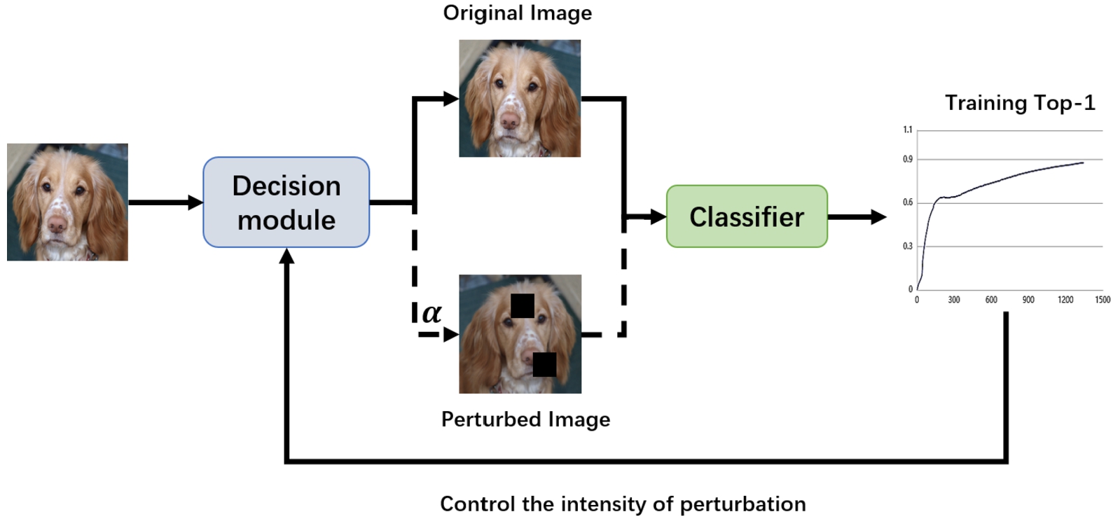
The flow chart of PairTraining is shown in Fig. 2. The input data is passed through the decision module to generate the corresponding image pair (image pairs consist of the original image and the disturbed image). The decision module is controlled to make different image disturbance strategies by the classifier in the top-1 of the training dataset. Where the top-1 indicates the category with the highest probability in the model prediction label. If this category is the same as the correct category, it is considered that the prediction is correct. The model then calculates the error of the original image and the disturbed image in turn. In the two calculations, the parameters of the model are the same. Finally, the gradient and update weight are calculated based on the error obtained by the two calculations.

PairTraining will increase training time. Although this method will add additional calculations during the model training phase, this will not change the network structure of the model. After the model training is completed, the infer speed of the model will not be affected. Next, PairTraining is described in detail.

Fig. 1.

Samples and classes on 2-D feature space. The red and blue dots represent two different categories. The black lines are the classification boundaries. The images on the left side of parts A and B are the performance of the training set, and the images on the right side are the performance of the test set. The light-colored dots in part B are the disturbed mapping points of the original data.

Fig. 2.

The overall process of PairTraining.

3.1. Decision module

The main role of the decision module is to select the appropriate image disturbance operations to generate disturbance images based on the previous round of training top-1. The decision module is based on the training accuracy top-1 β of the previous round, and the training process is divided into three stages. Different disturbance strategies are employed in each stage. The stages are divided as follows:

The qualitative stage ( $0 % ⩽ β ⩽ 25 %$ ). The model initially recognizes the classification task stage. In this stage, a weak disturbance strategy is used, that is, random clipping and random horizontal flipping are used as disturbance strategies.

The fine learning stage ( $25 % < β ⩽ 75 %$ ). The main stage of model training. During this stage, the model can gradually classify the labels with obvious classification boundaries accurately. In order to enhance the robustness of the model, the mask technology D-Mask is added on the basis of random clipping and random horizontal flipping at this stage.

The strengthening learning stage ( $75 % < β ⩽ 100 %$ ). At the current stage, the model further classifies the confusing categories and clarifies the category classification boundaries. Therefore, the aliasing technology D-Mix is added on the basis of random clipping and random horizontal flipping. The influence of other categories of image data is introduced to strengthen the model’s ability to classify easily confused categories.

At the beginning of each stage, a large number of interference operations will actually slow down the training convergence rate. And when the amount of data is large, using image pair training will bring huge computational load. Therefore, α is used to control whether to use the image disturbance technique to generate a contrast image. The calculation formula of α is as follows: $\begin{matrix} (2) & α = Max (\frac{1}{2}, \frac{β - β_{min}}{β_{max} - β_{min}}) \end{matrix}$ Where α is the probability of using image pair training, $β_{min}$ , $β_{max}$ are the minimum and maximum values of the corresponding β value interval in different learning stages (for example, in the qualitative learning stage, $β_{min} = 0$ , $β_{max} = 0.25$ ).

When β is closer to $β_{max}$ , α tends to be equal to 1, that is, all images need to be disturbed.

3.1.1. D-Mask

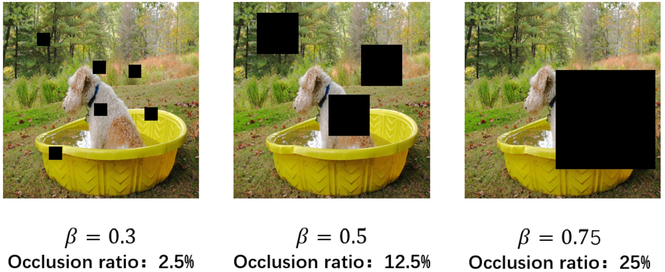
D-Mask is improved on the basis of Cutout. It can change the strategy of generating mask areas according to the change of training accuracy top-1 β. The D-Mask uses ${Mask}_{num}$ to control the number of masked areas. The height and width of each masked area are ${Mask}_{size}$ , and the calculation method is as follows: $\begin{array}{l} (3) & {Mask}_{num} = Max (Int (k (1 - \frac{1}{1 + \frac{2}{k - 1} e^{- k (β - β_{max})}})), 1) \\ (4) & {Mask}_{size} = Int (\sqrt{\frac{H * W * (β - β_{min})}{2 * {Mask}_{num}}}) \end{array}$ Where $Int$ represents the value rounded down, k is the coefficient of the number of masked areas (set $k = 6$ ), the number of masked areas can be controlled between $(0, k)$ , H, W are the height and width of the image, $β_{min} = 0.25$ , $β_{max} = 0.75$ .

${Mask}_{num}$ is negatively correlated with ${Mask}_{size}$ . As the training accuracy increases, the number of masked regions is gradually reduced and the area of a single masked region is gradually increased. This allows the model to implement a small-to-many masking strategy in the early stages of training, and is less susceptible to large-scale continuous masking. The purpose of this scheme is to reduce the possibility of convergence failure due to excessive disturbance during training. In the later stage of training, it is hoped to implement a single large-area shielding strategy to increase enough disturbance intensity for model training. At the same time, the maximum mask area is controlled between 0% and 25% due to the change of β (D-Mask randomly generates the position of the mask area, so overlap between different mask areas is allowed). The D-Mask effect is shown in Fig. 3. In order to more intuitively reflect what changes have D-Mask made on the basis of Cutout, the key differences between Cutout and D-Mask are shown in Table 1.

3.1.2. D-Mix

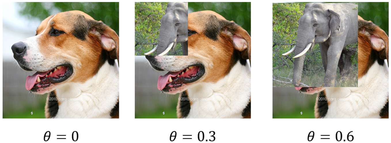
D-Mix makes adjustments on the basis of Cutmix. D-Mix cuts and aliases the sample images of different labels. The position of the clipping area is randomly generated. The size of the clipping area is related to the training accuracy β, and the image disturbance intensity is adjusted by the increase or decrease of the combination ratio θ. The D-Mix effect is shown in Fig. 4.

Fig. 3.

D-Mask effect demonstration.

Table 1

Comparison between Cutout and D-Mask

Method	Application scenario	Parameter setting
Cutout	This method is usually applied to the data pre-processing stage before model training. It is a common method for data enhancement.	$cut_num$ (int): The number of mask areas of each image. This is a fixed value. By default, n_holes = 1.
Cutout		$cut_length$ (int): The length (in pixels) of each square masked area. This is a fixed value that needs to be adjusted according to the data characteristics.
D-Mask	This method is applied to the model training phase, which can improve the effectiveness of training.	$mask_num$ (int): The number of mask areas of each image. This value will be dynamically adjusted according to the training top-1, with a range of 0–k (set $k = 6$ ).
D-Mask		$mask_length$ (int): The length (in pixels) of each square masked area. This value will be dynamically adjusted according to the size of the image, the training top-1, and the number of mask areas.

Fig. 4.

D-Mix effect demonstration.

D-Mix’s goal is to generate new training samples $(X_{mix}, Y_{mix})$ by combining two training samples $(X_{i}, Y_{i})$ and $(X_{j}, Y_{j})$ . The operation process of D-Mix can be expressed as: $\begin{array}{l} (5) & X_{mix} = M ⊙ X_{i} + (1 - M) ⊙ X_{j} \\ (6) & Y_{mix} = θ Y_{i} + (1 - θ) Y_{j} \\ (7) & θ = \frac{θ_{max}}{1 + e^{- γ (β - β_{min})}} \\ (8) & R_{h} = h * \sqrt{θ} \\ (9) & R_{w} = w * \sqrt{θ} \end{array}$ Where M represents a clipping region with a length of $R_{h}$ and a width of $R_{w}$ , and the position of this clipping area in the two pictures is the same. θ is the combination ratio. γ is the scaling factor, which controls the rate of increase of θ ( $γ = 50$ ). h and w are the length and width of the original pictures, respectively.

The value range of θ is between 0.3–0.6. The larger the proportion of clipping area, the greater the disturbance to the image, and the more difficult it is for the model to correctly identify the image.

In order to more intuitively reflect what changes have D-Mix made on the basis of Cutmix, the key differences between Cutmix and D-Mix are shown in Table 2.

Table 2

Comparison between Cutmix and D-Mix

Method	Application scenario	Parameter setting
Cutmix	This method is usually applied to the data pre-processing stage before model training. It is a common method for data enhancement.	The combination ratio θ between two data points is sampled from the beta distribution $Beta (α, α)$ .
D-Mix	This method is applied to the model training phase, which can improve the effectiveness of training.	The combination ratio θ will be dynamically adjusted according to the training top-1.

3.2. Loss function

Due to the diversity of CNN network structures, the loss functions used by different network structures may be different. Therefore, in order to increase the portability of PairTraining, only the loss of the input image pair is weighted. Take the cross-entropy loss function [29] as an example. With x representing the predicted value and $label$ representing the label value, the loss function of PairTraining can be expressed as: $\begin{array}{l} (10) & CEloss (x, label) = - log (\frac{exp (x [label])}{\sum_{i} exp (x [i])}) \\ (11) & Loss = ω * CEloss (x_{z}, {label}_{z}) + (1 - ω) * CEloss (x_{p}, {label}_{p}) \end{array}$

In the formula, the subscript z represents the original image of the image pair, and p represents the disturbed image. ω is the weighting coefficient, and ω can be dynamically adjusted with the performance of the model (this article sets $ω = 0.6$ ).

3.3. PairTraining overall process

The overall process of PairTraining is shown in Algorithm 1.

Algorithm 1:

PairTraining method for CNN image classification network training

4. Experiment

Experimental hardware link GPU: Tesla V100 32GBÕ4. The experimental software environment is paddlepaddle2.0. The pre-training models required for experiments are the official open-source data of paddlepaddle. The datasets used in the experiments include: the Oxford 102 Flowers, the CIFAR10, the CIFAR100 and the ILSVRC2012 (mini). We use multiple CNN network models to train on the above four datasets to verify the effectiveness of PairTraining (Section 4.2). The contribution of each main strategy of PairTraining is investigated using ablation experiments (Section 4.3).

4.1. Datasets

Oxford 102 Flowers

This dataset was released in 2008 by the Department of Engineering Sciences, University of Oxford, creating a 102-category dataset containing 102 flower categories. Each class contains 40 to 258 images.

CIFAR10

The dataset contains 60,000 32Õ32 color images in 10 categories, each containing 6,000 images. 50,000 images are used as the training set and 10,000 images are used as the test set.

CIFAR100

The dataset is an expanded version of CIFAR10, containing 60,000 32Õ32 color images, 100 categories, and each category contains 6,00 images. 50,000 images are used as the training set and 10,000 images are used as the test set.

ILSVRC2012 (mini)

The dataset is derived from the validation set of ILSVRC2012. The ILSVRC2012 is a subset of the ImageNet dataset. The dataset has a total of 50,000 images, 1000 categories, and 50 images of each type. The data is divided into 40,000 images as training set and 10,000 images as test set.

4.2. Experimental result

To test whether PairTraining has general applicability, we conduct experiments using 11 common different series of CNN models. These include AlexNet, VGGNet, DenseNet121, Inception series (GoogLeNet, Xception41 [5]), ResNet series (ResNet50, ResNet101, ResNet50_vd, ResNet101_vd) and mobile series model (MobileNetV3 [12], ShuffleNetV2 [17]). The performances of all models on Oxford 102 Flowers, CIFAR10, CIFAR100 and ILSVRC2012 (mini) datasets are shown in Table 3. (Note: Since ILSVRC2012 (mini) has many categories and few pictures of each category, it is necessary to load the pre-training model for training, otherwise the model will be difficult to converge.)

Table 3
Model performance comparison using different training methods

Model Flowers CIFAR10 CIFAR100 ILSVRC2012 (mini)

top-1 (%) top-1 (%) top-1 (%) top-1 (%) top-5 (%)

AlexNet 77.3 89.64 69.33 55.31 78.78

AlexNet (PairTraining) 79.75 ( $↑$ 2.45) 90.71 ( $↑$ 1.07) 70.42 ( $↑$ 1.09) 55.44 ( $↑$ 0.13) 80.13 ( $↑$ 1.35)

VGG16 – 93.25 71.34 71.3 90.37

VGG16 (PairTraining) – 93.59 ( $↑$ 0.34) 72.49 ( $↑$ 1.15) 71.97 ( $↑$ 0.67) 91.74 ( $↑$ 1.37)

GoogLeNet 80.27 92.55 70.34 68.81 87.9

GoogLeNet (PairTraining) 81.58 ( $↑$ 1.31) 93.69 ( $↑$ 1.14) 72.08 ( $↑$ 1.74) 70.18(↑1.37) 89.86 ( $↑$ 1.96)

Xception41 92.37 94.65 75.46 78.4 92.66

Xception41 (PairTraining) 93.40 ( $↑$ 0.93) 95.41 ( $↑$ 0.76) 77.40 ( $↑$ 1.94) 79.00 ( $↑$ 0.6) 94.14 ( $↑$ 1.48)

ResNet50 82.21 93.84 71.34 75.36 91.69

ResNet50 (PairTraining) 83.53 ( $↑$ 1.32) 95.27 ( $↑$ 1.43) 72.75(↑1.39) 76.13 ( $↑$ 0.77) 93.91 ( $↑$ 2.22)

ResNet101 81.36 93.28 72.93 76.32 92.35

ResNet101 (PairTraining) 82.54 ( $↑$ 1.18) 93.91 ( $↑$ 0.63) 74.63 ( $↑$ 1.7) 77.14 ( $↑$ 0.82) 94.37 ( $↑$ 2.02)

ResNet50_vd 85.87 95.31 75.84 77.86 93.81

ResNet50_vd (PairTraining) 87.25 ( $↑$ 1.38) 96.02 ( $↑$ 0.71) 77.96 ( $↑$ 2.12) 78.47 ( $↑$ 0.61) 95.69 ( $↑$ 1.88)

ResNet101_vd 83.7 94.16 77.15 79.38 93.42

ResNet101_vd (PairTraining) 85.03 ( $↑$ 1.33) 95.32 ( $↑$ 1.16) 78.39 ( $↑$ 1.24) 80.03 ( $↑$ 0.65) 95.89 ( $↑$ 2.47)

DenseNet121 78.54 94.83 76.28 73.14 91.2

DenseNet121 (PairTraining) 81.27 ( $↑$ 2.73) 95.16 ( $↑$ 0.33) 77.68 ( $↑$ 1.4) 73.94 ( $↑$ 0.8) 93.3 ( $↑$ 2.1)

MobileNetV3_large_x1_0 77.62 93.85 72.34 74.79 89.42

MobileNetV3_large_x1_0 (PairTraining) 79.54 ( $↑$ 1.92) 95.42 ( $↑$ 1.57) 73.63 ( $↑$ 1.29) 75.50 ( $↑$ 0.71) 90.14 ( $↑$ 0.72)

ShuffleNetV2_x1_5 78.57 93.27 72.86 70.33 89.28

ShuffleNetV2_x1_5 (PairTraining) 80.73 ( $↑$ 2.16) 94.81 ( $↑$ 1.54) 74.57 ( $↑$ 1.71) 71.48 ( $↑$ 1.15) 91.14 ( $↑$ 1.86)

Model	Flowers	CIFAR10	CIFAR100	ILSVRC2012 (mini)
AlexNet	77.3	89.64	69.33	55.31	78.78
AlexNet (PairTraining)	79.75 ( $↑$ 2.45)	90.71 ( $↑$ 1.07)	70.42 ( $↑$ 1.09)	55.44 ( $↑$ 0.13)	80.13 ( $↑$ 1.35)
VGG16	–	93.25	71.34	71.3	90.37
VGG16 (PairTraining)	–	93.59 ( $↑$ 0.34)	72.49 ( $↑$ 1.15)	71.97 ( $↑$ 0.67)	91.74 ( $↑$ 1.37)
GoogLeNet	80.27	92.55	70.34	68.81	87.9
GoogLeNet (PairTraining)	81.58 ( $↑$ 1.31)	93.69 ( $↑$ 1.14)	72.08 ( $↑$ 1.74)	70.18(↑1.37)	89.86 ( $↑$ 1.96)
Xception41	92.37	94.65	75.46	78.4	92.66
Xception41 (PairTraining)	93.40 ( $↑$ 0.93)	95.41 ( $↑$ 0.76)	77.40 ( $↑$ 1.94)	79.00 ( $↑$ 0.6)	94.14 ( $↑$ 1.48)
ResNet50	82.21	93.84	71.34	75.36	91.69
ResNet50 (PairTraining)	83.53 ( $↑$ 1.32)	95.27 ( $↑$ 1.43)	72.75(↑1.39)	76.13 ( $↑$ 0.77)	93.91 ( $↑$ 2.22)
ResNet101	81.36	93.28	72.93	76.32	92.35
ResNet101 (PairTraining)	82.54 ( $↑$ 1.18)	93.91 ( $↑$ 0.63)	74.63 ( $↑$ 1.7)	77.14 ( $↑$ 0.82)	94.37 ( $↑$ 2.02)
ResNet50_vd	85.87	95.31	75.84	77.86	93.81
ResNet50_vd (PairTraining)	87.25 ( $↑$ 1.38)	96.02 ( $↑$ 0.71)	77.96 ( $↑$ 2.12)	78.47 ( $↑$ 0.61)	95.69 ( $↑$ 1.88)
ResNet101_vd	83.7	94.16	77.15	79.38	93.42
ResNet101_vd (PairTraining)	85.03 ( $↑$ 1.33)	95.32 ( $↑$ 1.16)	78.39 ( $↑$ 1.24)	80.03 ( $↑$ 0.65)	95.89 ( $↑$ 2.47)
DenseNet121	78.54	94.83	76.28	73.14	91.2
DenseNet121 (PairTraining)	81.27 ( $↑$ 2.73)	95.16 ( $↑$ 0.33)	77.68 ( $↑$ 1.4)	73.94 ( $↑$ 0.8)	93.3 ( $↑$ 2.1)
MobileNetV3_large_x1_0	77.62	93.85	72.34	74.79	89.42
MobileNetV3_large_x1_0 (PairTraining)	79.54 ( $↑$ 1.92)	95.42 ( $↑$ 1.57)	73.63 ( $↑$ 1.29)	75.50 ( $↑$ 0.71)	90.14 ( $↑$ 0.72)
ShuffleNetV2_x1_5	78.57	93.27	72.86	70.33	89.28
ShuffleNetV2_x1_5 (PairTraining)	80.73 ( $↑$ 2.16)	94.81 ( $↑$ 1.54)	74.57 ( $↑$ 1.71)	71.48 ( $↑$ 1.15)	91.14 ( $↑$ 1.86)

This section sets up three sets of experiments, which are the classification accuracy comparisons of the test set, the training process comparison, and the training cost comparison of the model using different training methods.

4.2.1. Classification accuracy comparison

The experimental results are shown in Table 3. Details of the model parameters involved in the experiment can be found in the Appendix, where:

top-1 indicates the category with the highest probability in the model prediction label. If this category is the same as the correct category, it is considered that the prediction is correct. Equivalent to classification accuracy.

top-5 indicates that the model predicts the top five categories with the highest probability, and the correct category in these categories is regarded as correct prediction.

Compared with the ordinary training method, the performance of 11 models was improved in the four datasets after training with PairTraining.

In the Oxford 102 Flowers dataset, after using the PairTraining method, the top-1 growth interval of different models is between 0.93% and 2.73%. Among them, the increase of AlexNet and DenseNet121 is very obvious, with an increase of 2.45% and 2.73% respectively. PairTraining has greatly improved the mobile series models. The characteristics of the mobile series models are that some of the accuracy is sacrificed in exchange for the lightweight of the model. The classification accuracy of the mobile series model is low. The top-1 of MobileNetV3 and ShuffleNetV2 increased by 1.92% and 2.16% respectively. These models with larger increases are because these models are prone to fall into the local optimal situation during classification. Their performance has a lot of room for improvement. PairTraining can better tap the potential of the model. The Xception41 model can better complete the classification task of this dataset. Therefore, the improvement of the model by the PairTraining method is relatively small. The model’s top-1 only grew by 0.9%. For the ResNet and ResNet_vd series models, the average accuracy increases around 1.2%.

The classification difficulty of CIFAR10 is lower, and the accuracy of all models can be maintained at a high level, so the performance increase of different models is small. The growth range of top-1 is between 0.33% and 1.57%. For models with poor classification performance, the improvement is more obvious. The models of the mobile series have increased a lot, and the top-1 of MobileNetV3 and ShuffleNetV2 have increased by 1.57% and 1.54% respectively.

The classification of CIFAR100 is difficult, AlexNet and VGG16 are difficult to fit the training data during training, and the top-1 of the training set fluctuates around 75%. This will affect whether the D-mix operation of PairTraining is performed. Their top-1 increased by 1.09% and 1.15% respectively. The growth rate is low compared to other models. All other models in the top-1 of the training set meet the D-mix operation conditions of the third stage. The top-1 growth range of these models is between 1.24% and 2.12%. The Xception41’s top-1 increased by 1.94%. The top-1 of ResNet50_vd increased by 2.12%. It can be seen from the comparison that the use of D-mix can improve the effectiveness of training and increase the classification accuracy of the model.

ILSVRC2012 (mini) has many classification categories, and the top-5 is added for comparative analysis. The limitation of the AlexNet network structure makes it difficult to fit the data to converge, and the D-mix operation cannot be triggered. The top-1 and the top-5 of AlexNet increased by 0.13% and 1.35% respectively. The top-1 of AlexNet basically remained unchanged, but the top-5 was significantly improved. The top-1 of the other 10 models have all been improved to a certain extent, and the growth range is between 0.6% and 1.37%. The growth rate of top-5 is more obvious, and the growth range is between 0.72% and 2.22%.

Multiple experiments can prove the effectiveness of PairTraining. The network structure of different models often determines the performance of the model. PairTraining cannot break through the maximum performance of the model, but it can better tap the potential of the model. In the Oxford 102 Flowers dataset, the top-1 has an average increase of 1.64%. In the CIFAR10 dataset, the top-1 has an average increase of 0.91%. In the CIFAR100 dataset, the top-1 has an average increase of 1.47%. In the ILSVRC2012 (mini) dataset, the top-1 has an average increase of 0.71%, and the top-5 has an average increase of 1.51%.

4.2.2. Training process comparison

The experimental model in this section is ResNet50_vd, and the dataset is Oxford 102 Flowers. Compare the Training loss curve, Training top-1 curve and Test top-1 curve after using the two training methods.

The training process of ResNet50_vd in the Oxford 102 Flowers is shown in Fig. 5. Compared with ordinary training methods, PairTraining will turn around when Training top-1 reaches 0.25 and 0.75. The loss value has a small upward trend, but it only takes a few rounds to resume the downward trend. This is because D-mask and D-mix use variable control methods, which do not instantaneously increase the intensity of violent disturbance at the beginning of each stage. Gradually increasing the disturbance level helps the Training loss to converge smoothly. The loss function of PairTraining has a slower downward trend and requires more steps to converge. But the final Training loss of PairTraining is smaller, and the Training top-1 is higher.

Fig. 5.

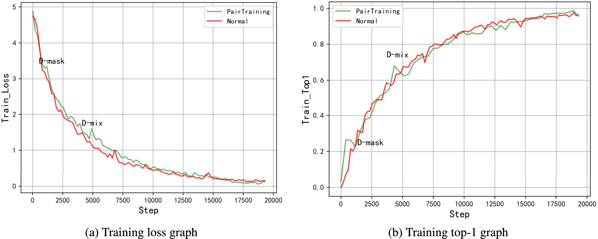
The training process of ResNet50_vd in the Oxford 102 Flowers.

The Test top-1 curve of the model is shown in Fig. 6. Although the loss of the common training method decreases faster, the Test top-1 obtained by the PairTraining method is better. Although the training top-1 of the two methods has a small gap, it can be seen from the test top-1 that after D-mix is used, the test top-1 has been improved rapidly. After using the PairTraining method, Test top-1 rose by 1.33%. The performance of the trained model becomes better.

Fig. 6.

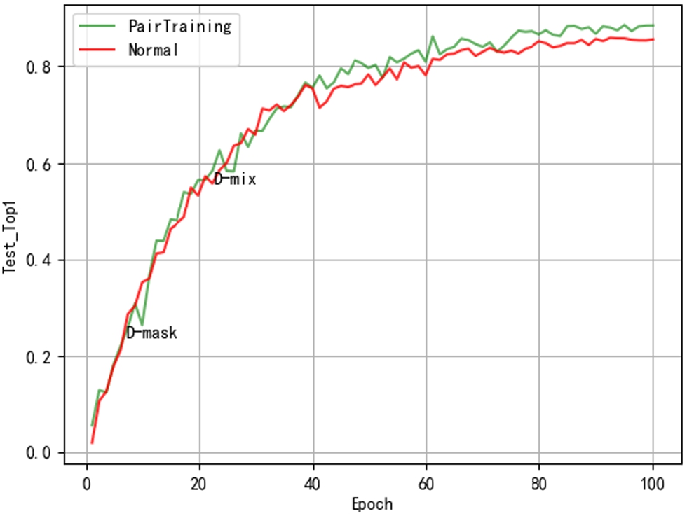
The Test top-1 graph of ResNet50_vd in the Oxford 102 Flowers.

4.2.3. Training cost comparison

Compared with the ordinary method, PairTraining will increase the extra computation. Each model has a different number of parameters. And the training epoch required for each model to converge is different. So using the average of each training epoch times for each model can compare the computational cost of the two training methods. All models are required to fully trigger the three stages of PairTraining, so CIFAR10 is used as the experimental dataset. The experimental results are shown in Fig. 7. The average training epoch times for all models increased between 15.78% and 28.14%. There is no significant increase in the amount of training computation. The α variable controls the extra computation introduced by training by controlling whether to use the PairTraining method. And in the CNN training process, the back-propagation process bears most of the computation. Since the image pairs share weights in the forward propagation process, the training process of PairTraining still only performs back propagation once. PairTraining only changes the training process and does not affect the inference phase of the model. Does not affect the inference speed of the model.

Fig. 7.

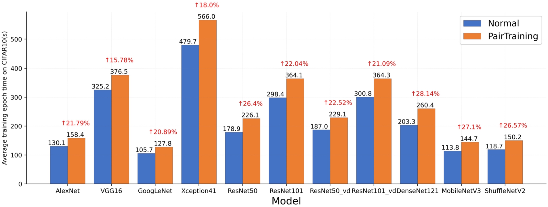
Average training epoch times for different models on CIFAR10.

Combining the data in Table 3 and Fig. 7, it is not difficult to find that PairTraining is more suitable for small and medium-sized data sets. The performance of PairTraining in the ILSVRC2012 (mini) with a large amount of data is relatively ordinary, and the top-1 has increased by about 0.7%on average. And the larger data sets mean higher training costs. At this time, if PairTraining is used, it will increase a lot of training cost. And for small and medium-sized data sets, the classification model with complex network structure is not the best choice. Such as ResNet101, ResNet101_vd and DenseNet121 in small and medium-sized data sets are not prominent. PairTraining does not break through the performance limit of the classification model. Therefore, if the selected classification model is not suitable for the characteristics of the data set, the use of PairTraining will not completely change this situation, it can only play a slight optimization purpose. Blind use of PairTraining will add additional training costs. Before using PairTraining, it is recommended to use normal training methods to find the appropriate classification model. After finding a suitable classification model, PairTraining is used for further tuning.

4.3. Ablation experiment

In order to test whether each component of PairTraining is reasonable and effective, an ablation experiment is designed. The model used in the experiment is ResNet50_vd.

4.3.1. Component testing

The ablation experimental data of each component is shown in Table 4. The stage 1 to 3 in the table correspond respectively to the qualitative stage, the fine learning stage and the strengthening learning stage. The strategy 1 in the table represents the normal training scheme, and the strategy 8 represents the PairTraining scheme. The Strategies 2 to 7 are control experiments. In the table, RF means random crop and random horizontal flip. All the Cutout methods in the table use the same parameter (set $cut_num = 1$ , $cut_length = 40$ ). The combination ratio θ of all Cutmix methods in the table conforms to the beta distribution $Beta (α, α)$ , and α is set to 1.

The random crop and random horizontal flip has little effect on training results. Image disturbance that are too small do not improve model performance. The Cutout and Cutmix methods have a small increase in model performance in the Flowers and the Cifar10 with fewer label categories. However, For the Cifar100 and the ILSVRC2012 (mini) with more label categories, the classification accuracy of the model decreases. This is because adding too much disturbance to a dataset with high classification difficulty will lead to difficulty in model training, and the loss value of the model is difficult to converge. Among them, Cutout is less disturbed than Cutmix, so the top-1 of Cifar100 and ILSVRC2012 (mini) has a smaller decrease, with a decrease of 0.29% and 0.38% respectively. Cutmix has poor model training results due to excessive interference with classification. The top-1 in Cifar100 dropped 2.19%. The top-1 in ILSVRC2012 (mini) dropped by 5.53%.

Relatively speaking, D-Mask and D-Mix are stable. There is no situation where the performance of the model is degraded due to excessive disturbance. Compared with Cutout and Cutmix, the improvement effect of model performance is better. Among the single disturbance strategies, D-Mix is the best, and the top-1 of each data set has been significantly increased. In particular, the top-5 of ILSVRC2012 (mini) has been greatly improved by 1.53%. Appropriately sized image disturbance is critical to the success of model training.

Table 4
Performance comparison of RESNET50_VD using different training methods

Method Flowers CIFAR10 CIFAR100 ILSVRC2012 (mini)

Stage 1 Stage 2 Stage 3 top-1 (%) top-1 (%) top-1 (%) top-1 (%) top-5 (%)

1 – – – 95.87 95.31 75.84 77.86 93.81

2 RF – – 95.89 (↑0.02) 95.29 (↓0.02) 75.82 (↓0.02) 77.87 (↑0.01) 93.82 (↑0.01)

3 RF Cutout 96.17 (↑0.30) 95.55 (↑0.24) 75.55 (↓0.29) 77.48 (↓0.38) 93.62 (↓0.19)

4 RF D-Mask – 96.52 (↑0.65) 95.68 (↑0.37) 76.35 (↑0.51) 78.05 (↑0.19) 94.17 (↑0.36)

5 RF – Cutmix 94.04 (↑0.17) 95.47 (↑0.16) 73.65 (↓2.19) 72.33 (↓5.53) 91.78 (↓2.03)

6 RF – D-Mix 96.41 (↑0.54) 95.89 (↑0.58) 76.58 (↑0.74) 78.09 (↑0.23) 95.34 (↑1.53)

7 RF Cutout Cutmix 95.18 (↓0.69) 94.58 (↓0.73) 74.01 (↓1.83) 74.34 (↓3.52) 92.01 (↓1.80)

8 RF D-Mask D-Mix 97.25 ( $↑$ 1.28) 96.02 ( $↑$ 0.71) 77.96 ( $↑$ 2.12) 78.47 ( $↑$ 0.61) 95.69 ( $↑$ 1.88)

	Method	Flowers	CIFAR10	CIFAR100	ILSVRC2012 (mini)
1	–	–	–	95.87	95.31	75.84	77.86	93.81
2	RF	–	–	95.89 (↑0.02)	95.29 (↓0.02)	75.82 (↓0.02)	77.87 (↑0.01)	93.82 (↑0.01)
3	RF	Cutout		96.17 (↑0.30)	95.55 (↑0.24)	75.55 (↓0.29)	77.48 (↓0.38)	93.62 (↓0.19)
4	RF	D-Mask	–	96.52 (↑0.65)	95.68 (↑0.37)	76.35 (↑0.51)	78.05 (↑0.19)	94.17 (↑0.36)
5	RF	–	Cutmix	94.04 (↑0.17)	95.47 (↑0.16)	73.65 (↓2.19)	72.33 (↓5.53)	91.78 (↓2.03)
6	RF	–	D-Mix	96.41 (↑0.54)	95.89 (↑0.58)	76.58 (↑0.74)	78.09 (↑0.23)	95.34 (↑1.53)
7	RF	Cutout	Cutmix	95.18 (↓0.69)	94.58 (↓0.73)	74.01 (↓1.83)	74.34 (↓3.52)	92.01 (↓1.80)
8	RF	D-Mask	D-Mix	97.25 ( $↑$ 1.28)	96.02 ( $↑$ 0.71)	77.96 ( $↑$ 2.12)	78.47 ( $↑$ 0.61)	95.69 ( $↑$ 1.88)

4.3.2. Weighted coefficient of loss function

Table 5 shows the influence of the weighting coefficient ω of the loss function in PairTraining on the final model performance with different values. Different sizes of ω mean the weight of the classification results of disturbed images during training. The larger the ω, the more emphasis is placed on considering the classification results of disturbed images. When $ω = 1$ , PairTraining is equivalent to the normal method, and the model performance data is the baseline data. When $ω = 0.5$ , in the Flowers dataset, top-1 has a large drop. Compared with the baseline data, it drops by 1.52%. This is due to the fact that there are fewer image samples in the Flowers dataset, which leads to the poor anti-disturbance ability of the trained model. When $ω = 0.5$ , for the Cifar100 and ILSVRC2012 (mini) datasets with higher classification difficulty, the performance of the model is improved significantly. Among them, the top-5 of the ILSVRC2012 (mini) dataset is the highest, which is 2.27% higher than the baseline data. $ω = 0.6$ has the most stable performance in all datasets. As ω increases, all model data gradually approach the baseline data. The value of ω can be determined by the specific data set situation. It can be seen from the experimental data that for data sets with fewer data samples and classification labels, the ω value can be appropriately increased to ensure stable training. For datasets with more data samples and classification labels, the ω value can be appropriately reduced. Try setting $ω = 0.6$ first.

Table 5
Influence of weighting coefficient on performance of RESNET50_VD

Ablation Flowers CIFAR10 CIFAR100 ILSVRC2012 (mini)

top-1 (%) top-1 (%) top-1 (%) top-1 (%) top-5 (%)

$ω = 0.5$ 84.35 (↓1.52) 95.19 (↓0.12) 77. 74 (↑1.90) 78.51 (↑0.65) 96.08 (↑2.27)

$ω = 0.6$ 87.25 ( $↑$ 1.38) 96.02 ( $↑$ 0.71) 77.96 ( $↑$ 2.12) 78.47 ( $↑$ 0.61) 95.69 ( $↑$ 1.88)

$ω = 0.7$ 87.00 (↑1.13) 96.16 (↑0.85) 77.41 (↑1.57) 78.33 (↑0.47) 95.11 (↑1.30)

$ω = 0.8$ 86.39 (↑0.52) 95.63 (↑0.32) 76.96 (↑1.12) 78.09 (↑0.23) 94.30 (↑0.49)

$ω = 0.9$ 86.15 (↑0.28) 95.51 (↑0.20) 76.12 (↑0.28) 78.10 (↑0.24) 93.94 (↑0.13)

$ω = 1$ 85.87 95.31 75.84 77.86 93.81

Ablation	Flowers	CIFAR10	CIFAR100	ILSVRC2012 (mini)
$ω = 0.5$	84.35 (↓1.52)	95.19 (↓0.12)	77. 74 (↑1.90)	78.51 (↑0.65)	96.08 (↑2.27)
$ω = 0.6$	87.25 ( $↑$ 1.38)	96.02 ( $↑$ 0.71)	77.96 ( $↑$ 2.12)	78.47 ( $↑$ 0.61)	95.69 ( $↑$ 1.88)
$ω = 0.7$	87.00 (↑1.13)	96.16 (↑0.85)	77.41 (↑1.57)	78.33 (↑0.47)	95.11 (↑1.30)
$ω = 0.8$	86.39 (↑0.52)	95.63 (↑0.32)	76.96 (↑1.12)	78.09 (↑0.23)	94.30 (↑0.49)
$ω = 0.9$	86.15 (↑0.28)	95.51 (↑0.20)	76.12 (↑0.28)	78.10 (↑0.24)	93.94 (↑0.13)
$ω = 1$	85.87	95.31	75.84	77.86	93.81

5. Conclusion and future work

Aiming at the problems of poor flexibility, low utilization of labeled samples and low generalization degree of common CNN training methods, this paper proposes a training method PairTraining, which uses image disturbance to generate contrast images and train them in pairs with the original images. Furthermore, D-Mask and D-Mix methods are proposed, which can dynamically change the disturbance parameters with the training degree, which can effectively and reasonably combine the image disturbance with the training process. PairTraining effectively improves the training effectiveness of the model by using image disturbance and the idea of consistency regularization. PairTraining greatly improves the accuracy and stability of the model when dealing with image classification at the cost of a small increase in training cost. In the experiments, the performance of the multi-group classification models on different datasets has been improved. PairTraining also puts forward new ideas for the optimization of training methods.

The current experiments of this method are all in the image classification task, and the effectiveness in the fields of object detection and semantic segmentation has not been explored. Future work will be tested in areas such as object detection and semantic segmentation to further improve the training scheme.

Footnotes

Acknowledgement

This work was supported in part by Scientific Research Projects of the Education Department of Liaoning Province (No. LJKZ0537, No. J2020113).

Model training parameters

The training parameters of the model on the Oxford 102 Flowers and the CIFAR10 are shown in Table 6. The training parameters of the model on the CIFAR10 and the ILSVRC2012 (mini) are shown in Table 7. Mainly use the Momentum-Optimizer (momentum = 0.9). The regular term mainly uses L2.

References

Berthelot,

Carlini,

E.D.

Cubuk,

Kurakin,

Sohn,

Zhang and

Raffel, Remixmatch: Semi-supervised learning with distribution alignment and augmentation anchoring, 2019, arXiv preprint arXiv:1911.09785.

Berthelot,

Carlini,

Goodfellow,

Papernot,

Oliver and

C.A.

Raffel, Mixmatch: A holistic approach to semi-supervised learning, Advances in Neural Information Processing Systems 32 (2019).

Chapelle,

Scholkopf and

Zien, Semi-supervised learning (Chapelle, O. et al., eds.; 2006) [book reviews], IEEE Transactions on Neural Networks 20(3) (2009), 542–542. doi:10.1109/TNN.2009.2015974.

Chen,

Liu,

Zhao and

Jia, Gridmask data augmentation, 2020, arXiv preprint arXiv:2001.04086.

Chollet, Xception: Deep learning with depthwise separable convolutions, in: Proceedings of the IEEE Conference on Computer Vision and Pattern Recognition, 2017, pp. 1251–1258.

E.D.

Cubuk,

Zoph,

Mane,

Vasudevan and

Q.V.

Le, Autoaugment: Learning augmentation policies from data, 2018, arXiv preprint arXiv:1805.09501.

E.D.

Cubuk,

Zoph,

Shlens and

Q.V.

Le, Randaugment: Practical automated data augmentation with a reduced search space, in: Proceedings of the IEEE/CVF Conference on Computer Vision and Pattern Recognition Workshops, 2020, pp. 702–703.

DeVries and

G.W.

Taylor, Improved regularization of convolutional neural networks with cutout, 2017, arXiv preprint arXiv:1708.04552.

M.C.

Dickson,

A.S.

Bosman and

K.M.

Malan, Hybridised loss functions for improved neural network generalisation, in: Pan-African Artificial Intelligence and Smart Systems Conference, Springer, 2021, pp. 169–181.

10.

R.H.R.

Hahnloser,

Sarpeshkar,

M.A.

Mahowald,

R.J.

Douglas and

H.S.

Seung, Digital selection and analogue amplification coexist in a cortex-inspired silicon circuit, Nature 405(6789) (2000), 947–951. doi:10.1038/35016072.

11.

He,

Zhang,

Ren and

Sun, Deep residual learning for image recognition, in: Proceedings of the IEEE Conference on Computer Vision and Pattern Recognition, 2016, pp. 770–778.

12.

Howard,

Sandler,

Chu,

L.-C.

Chen,

Tan,

Wang,

Zhu,

Pang,

Vasudevan et al., Searching for mobilenetv3, in: Proceedings of the IEEE/CVF International Conference on Computer Vision, 2019, pp. 1314–1324.

13.

Huang,

Liu,

Van Der Maaten and

K.Q.

Weinberger, Densely connected convolutional networks, in: Proceedings of the IEEE Conference on Computer Vision and Pattern Recognition, 2017, pp. 4700–4708.

14.

Klambauer,

Unterthiner,

Mayr and

Hochreiter, Self-normalizing neural networks, Advances in neural information processing systems 30 (2017).

15.

Krizhevsky,

Sutskever and

G.E.

Hinton, Imagenet classification with deep convolutional neural networks, Advances in neural information processing systems 25 (2012).

16.

LeCun,

Bottou,

Bengio and

Haffner, Gradient-based learning applied to document recognition, Proceedings of the IEEE 86(11) (1998), 2278–2324. doi:10.1109/5.726791.

17.

Ma,

Zhang,

H.-T.

Zheng and

Sun, Shufflenet v2: Practical guidelines for efficient CNN architecture design, in: Proceedings of the European Conference on Computer Vision (ECCV), 2018, pp. 116–131.

18.

Ramachandran,

Zoph and

Q.V.

Le, Searching for activation functions, 2017, arXiv preprint arXiv:1710.05941.

19.

Sajjadi,

Javanmardi and

Tasdizen, Regularization with stochastic transformations and perturbations for deep semi-supervised learning, Advances in neural information processing systems 29 (2016).

20.

Simonyan and

Zisserman, Very deep convolutional networks for large-scale image recognition, 2014, arXiv preprint arXiv:1409.1556.

21.

K.K.

Singh,

Yu,

Sarmasi,

Pradeep and

Y.J.

Lee, Hide-and-seek: A data augmentation technique for weakly-supervised localization and beyond, 2018, arXiv preprint arXiv:1811.02545.

22.

Sohn,

Berthelot,

Carlini,

Zhang,

C.A.

Raffel,

E.D.

Cubuk ,

Kurakin and

C.-L.

Li , Fixmatch: Simplifying semi-supervised learning with consistency and confidence, Advances in Neural Information Processing Systems 33 (2020), 596–608.

23.

Srivastava,

Hinton,

Krizhevsky,

Sutskever and

Salakhutdinov, Dropout: A simple way to prevent neural networks from overfitting, The journal of machine learning research 15(1) (2014), 1929–1958.

24.

Szegedy,

Liu,

Jia,

Sermanet,

Reed,

Anguelov,

Erhan,

Vanhoucke and

Rabinovich, Going deeper with convolutions, in: Proceedings of the IEEE Conference on Computer Vision and Pattern Recognition, 2015, pp. 1–9.

25.

Xie,

Dai,

Hovy,

Luong and

Le, Unsupervised data augmentation for consistency training, Advances in Neural Information Processing Systems 33 (2020), 6256–6268.

26.

Xie,

M.-T.

Luong,

Hovy and

Q.V.

Le, Self-training with noisy student improves imagenet classification, in: Proceedings of the IEEE/CVF Conference on Computer Vision and Pattern Recognition, 2020, pp. 10687–10698.

27.

Yun,

Han,

S.J.

Oh,

Chun,

Choe and

Yoo, Cutmix: Regularization strategy to train strong classifiers with localizable features, in: Proceedings of the IEEE/CVF International Conference on Computer Vision, 2019, pp. 6023–6032.

28.

Zhang,

Cisse,

Y.N.

Dauphin and

Lopez-Paz, mixup: Beyond empirical risk minimization, 2017, arXiv preprint arXiv:1710.09412.

29.

Zhang and

Sabuncu, Generalized cross entropy loss for training deep neural networks with noisy labels, Advances in neural information processing systems 31 (2018).

30.

Zhong,

Zheng,

Kang,

Li and

Yang, Random erasing data augmentation, in: Proceedings of the AAAI Conference on Artificial Intelligence, Vol. 34, 2020, pp. 13001–13008.