Variational method for wide area surveillance

Abstract

In this paper, a novel variational method is introduced for multi-object tracking in a network of cameras. In a camera network, objects are tracked by each camera using any of conventional algorithms and their tracks are extracted. Each extracted track is called a tracklet. The extracted tracklets are the inputs to our proposed method. Our objective in this paper is to associate the corresponding tracklets of an object and present the persistent trace of all objects. The association is formulated and solved using a variational energy function, which is based on appearance and motion model of objects. The optimization is realized by, first converting the variational energy function into an Ordinary Differential Equation (ODE) employing the Euler-Lagrange equation; then, the ODE is solved by numerical methods. The proposed method is evaluated on three well known real datasets and one synthetic dataset. The performance of our method is compared with the state of the art methods, employing the conventional metrics and under less restrictive assumption, and superiority of our method is demonstrated.

Keywords

Variational method multi-object tracking camera network tracking wide area monitoring

1. Introduction

In recent years, demands for monitoring wide geographic area, for different applications, is increased. The visual monitoring is realized by utilizing a network of cameras. In order to take advantage of these systems more efficiently, autonomous tools are required [15,22]. An important component of this autonomous system is an algorithm that tracks objects in different cameras persistently. The persistent tracking of objects includes of two steps: 1-Tracking objects in each camera and extracting the tracklets, 2-associating the tracklets for each object.

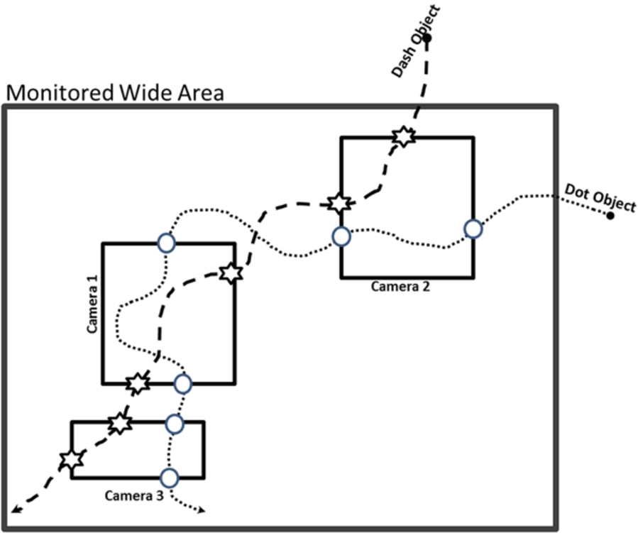
Various algorithms have been proposed for the implementation of the first step and remarkable progresses have been introduced in this area of research [32]. However, for the subject of second step, which is a new area of research, less research has been conducted [21]. In this paper, it is assumed that the tracklets are obtained accurately in the first step using any preferred methods [32]. The persistent tracking of objects within a camera of network are dealt in [1,12,14,20,21,24–26,30,31]. In [21,24,25] by combining short term feature correspondences across the cameras and using the long-term feature dependency models, a novel multi-objective optimization framework has been proposed. In this method, the similarities between features observed at different cameras are adapted based on the long-term models then a stochastically optimal path for each person is extracted. In [20], a new representation model has been proposed to extract tracklets followed by a statistical method for associating the tracklets. In [12], a statistical model has been proposed based on appearance and motion of the objects and the maximum a posterior (MAP) is used to solve the correspondence. In [26] a planar tracking correspondence model (TCM) is presented for addressing the association problem. In this work, the first fully automatic methods for estimating the planar TCM in large camera networks is introduced. The planar TCM is estimated only based on the overlapping camera’s correspondence. In [14] the authors have presented a method for learning the model of the camera network topology and using this model for tracking targets across blind regions. These blind regions are exist due to either large occlusions or separation of the camera views. In this work, it is assumed that the topology of cameras in camera network and transition model of objects between cameras are trainable. In [1] the camera networks are categorized into three groups. Then, the statistical methods are presented for associating based on the appearance and motion model of objects. In [30] a Petri Net based model is presented which associate the tracklets based on the color and gray histogram, local binary bitmap features and some estimated motion models. In [31], the appearance model of objects is extracted in different poses, different lighting situations and different cameras, then, the objects are tracked based on these extracted models. The common approach for associating the tracklets is performed by, first establishing all possible hypothesizes and then each hypothesis is evaluated based on different models in order to determine the best ones. The complexity of data association hypothesizes grows exponentially [6] with time and the number of the cameras and objects. Most of the related works, which are proposed to deal with this problem, use two restricted assumptions in order to relax this challenge. The first restriction assumes the topology of the cameras in the camera network is known. For example in [12,21,24] it is assumed that the camera network has known or trainable topology and movement trend of objects between each pair of cameras are also known. However, this assumption is not applied globally. The second restriction is to assume that the correspondences obey the Markovian model as a conditional dependency [12,20,21,24]. In other works, this assumption is addressed by introducing a second objective to the model. Considering this restrictive assumption when pruning the solution space, in some cases, it may converge to a false solution. To substantiate this claim, we use the scenario presented in Fig. 1. In this scenario, assume there are two objects that are appeared in the view point of camera 3 following their exiting from the view of camera 1. If the first order Markovian model be used for extracting the persistent trace of two objects in this scenario, the error which is shown in Fig. 2 will affect the final results. This phenomenon happens because in first order Markovian model, the next state of the model is related to only the first previous state of the model. While, if all state of the model, which in our problem means all tracklets of the persistent trace, be used in association process, extracting the true solution is possible. In this paper, a novel model is proposed for solving the problem of tracklet association problem without imposing the mentioned restrictive assumptions.

Fig. 1.

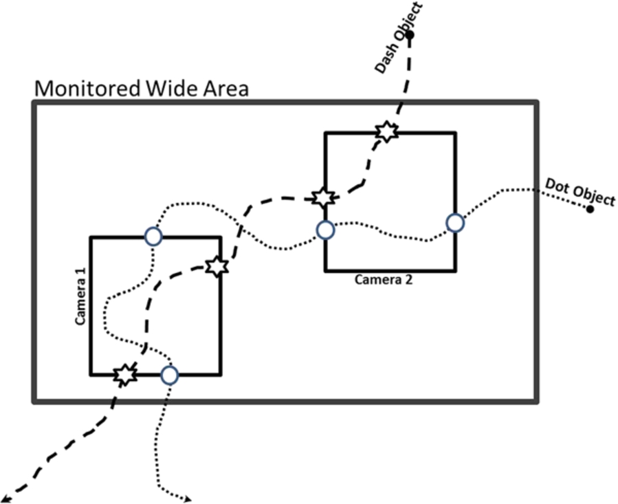
A sample of the persistent tracking problem.

Fig. 2.

Incorrect solution of persistent tracking of the objects.

This problem is an illustration of ill-posed inverse problem [2] where the tracklets are the observation and assumed to be known and the persistent trace is the ideal output and unknown (more details are presented in Appendix B). On the other hand, the variational model is an effective solution for solving the ill-posed inverse problem [28,29]. This model is commonly used for solving the ill-posed inverse problem in the scope of image processing and computer vision [8,19,27]. Motivated by the above mentioned discussions, this paper proposes a novel variational method for solving the problem without introducing the restrictive assumptions. In the proposed method, we have assumed that for each camera a tracking algorithm is used and the tracklets of objects are extracted. The collected tracklets of all cameras are considered as input to our problem. Then, our objective is to use these tracklets in order to extract persistent trace of the objects based on the appearance and motion model.

The rest of this paper is organized as follows. In Section 2 the problem is formulated. In Section 2.1 the proposed variational method is presented. In Section 2.3 the numerical solution for solving the variational method is considered. The experimental results, which are achieved using real and synthetic video sequence, are considered in Section 3 and finally, a brief summary of the proposed method and achieved results are presented in Section 4.

2. Problem formulation

The notations which are used throughout this paper, are presented in Table 1. Our problem is to track the persistent trace of the observed object over a network of cameras. In this problem, we have a camera network with

k > 1

cameras and the calibration parameters which project each point of the image from image plane to the world ground plane which is denoted by

C_{M}

and assumed to be known. There are

n > 1

objects in the area that is covered by the camera network, and is unknown. Furthermore, the tracking of each camera has been performed and all tracklets are extracted and denoted by a set T,

| T | > 2

. The incident time of all tracklets, are within the window time

[t_{s}, t_{e}]

. In this problem, our desire is to extract persistent trace of the objects

R = {r_{1}, \dots, r_{n}}

based on the extracted tracklets T. Hence, we can formulate the problem as a function described by,

\begin{matrix} (1) & R = Tracer (T, C_{M}), \end{matrix}

which means that the tracer algorithm receives the tracklets and camera parameters as inputs and present persistent trace as the output. As stated in Section 1, this persistent tracking problem is an ill-posed inverse problem [2], and a variational method is an effective solution for solving the ill-posed inverse problem [28,29]. In this paper, our main contribution is to propose a variational model for solving this problem.

Table 1
Problem notations

$C_{M}$	Calibration parameters of all cameras
$t_{s}$	Start tracking time windows
$t_{e}$	End tracking time windows
T	Tracklets set of all cameras
$τ_{l}$	The lth tracklet of the tracklets set T
R	Persistent trace of all objects
$r_{i}$	Persistent trace of the ith object $r_{i} \in R$
$F_{A} (\cdot)$	Appearance model (the color histogram (RGB))
$F_{M} (\cdot)$	Motion model (the orientation and the speed change rate of the object)
$DistA (\cdot)$	The distance measure between two appearance models (the Hellinger [16] distance)
$DistM (\cdot)$	The distance measure between two motion models (the norm-one)
n	Count of moving objects
b	Count of tracked objects by the algorithm
$ϕ_{i}$	Level set representation of $r_{i}$
$\| \cdot \|$	The cardinality of the set

2.1. Variational model

The persistent trace of an object, i.e. $r_{i}$ the persistent trace of ith object, is obtained by introducing a variational function and it is then solved by an optimization process. The persistent tracking of other objects are evaluated by repeating and iterating the optimization process. Let us define $r_{i} \subseteq T$ as the persistent trace of object ith that all of its tracklets are captured by a camera network. The optimization problem is solved by minimizing the energy function that is presented by, $\begin{array}{l} J [r_{i}] & = λ_{1} \times \sum_{τ_{l} \in T} CLS (r_{i}, τ_{l}) \\ (2) & + λ_{2} \times \sum_{τ_{l} \in r_{i}} SM (r_{i}, τ_{l}), \end{array}$ where $CLS (\cdot)$ is the closeness part of the energy function that leads to a persistent trace which includes similar tracklets based on an appearance model, $SM (\cdot)$ is the smoothness part of the energy function that leads to a persistent trace with minimum variation and $λ_{1} > 0$ and $λ_{2} > 0$ are fixed parameters. The closeness part $CLS (\cdot)$ of Eq. (2) is defined by, $\begin{matrix} (3) & CLS (r_{i}, τ_{l}) = \{\begin{matrix} DistA (F_{A} (τ_{l}), F_{A} (r_{i})) & τ_{l} \in r_{i} \\ (1 - DistA (F_{A} (τ_{l}), F_{A} (r_{i})) & τ_{l} \notin r_{i}, \end{matrix} \end{matrix}$ where $F_{A} (\cdot)$ is the appearance model of the object and $DistA (\cdot)$ is the distance measure between two appearance models. Also, $F_{A} (τ_{l})$ is the mean appearance model of the tracklet $τ_{l}$ and $F_{A} (r_{i})$ is the mean appearance model of the ith object. The closeness part of the model is minimized when the tracklet $τ_{l}$ which is assigned to the persistent trace of object ith has similar appearance to the other tracklets which have already been assigned to this object. Furthermore, the $SM (\cdot)$ is defined as follow, $\begin{array}{l} SM (r_{i}, τ_{l}) \\ = V (r_{i}, τ_{l}) + VV (r_{i}, τ_{l}) \\ (4) & + {[DistA (F_{A} (τ_{l}), F_{A} (r_{i / τ_{l}})) - {MeanF}_{A} (r_{i / τ_{l}})]}^{2}, \end{array}$ where, $\begin{array}{l} V (r_{i}, τ_{l}) \\ = {[DistA (F_{A} (τ_{l}), F_{A} (r_{i})) - {MeanF}_{A} (r_{i})]}^{2} \\ (5) & + {[DistM (F_{M} (τ_{l}), F_{M} (r_{i})) - {MeanF}_{M} (r_{i})]}^{2}, \end{array}$ and, $\begin{array}{l} VV (r_{i}, τ_{l}) \\ = \sum_{τ_{j} \in r_{i}} [‖ {[DistA (F_{A} (τ_{j}), F_{A} (r_{i})) - {MeanF}_{A} (r_{i})]}^{2} \\ - {[DistA (F_{A} (τ_{j}), F_{A} (r_{i / τ_{l}})) - {MeanF}_{A} (r_{i / τ_{l}})]}^{2} ‖ \\ + ‖ {[DistM (F_{M} (τ_{j}), F_{M} (r_{i})) - {MeanF}_{M} (r_{i})]}^{2} \\ - [DistM (F_{M} (τ_{j}), F_{M} (r_{i / τ_{l}})) \\ (6) & - {MeanF}_{M} (r_{i / τ_{l}})]^{2} ‖], \end{array}$ where $F_{M} (\cdot)$ is a motion model of the object, $F_{M} (τ_{l})$ is the mean motion model of the tracklet $τ_{l}$ , $F_{M} (r_{i})$ is the mean motion model of the ith object, $DistM (\cdot)$ is the distance measure between two motion models, $r_{i / τ_{l}}$ is a set of all tracklets in $r_{i}$ except $τ_{l}$ , and ${MeanF}_{A} (\cdot)$ and ${MeanF}_{M} (\cdot)$ are the mean distance measure and are defined as, $\begin{array}{l} {MeanF}_{A} (r_{i}) = \frac{1}{| r_{i} |} \times \sum_{τ_{j} \in r_{i}} DistA (F_{A} (τ_{j}), F_{A} (r_{i})) \\ (7) & {MeanF}_{M} (r_{i}) = \frac{1}{| r_{i} |} \times \sum_{τ_{j} \in r_{i}} DistM (F_{M} (τ_{j}), F_{M} (r_{i})) . \end{array}$

The smoothness part of the energy function is minimized when the assigned tracklets to the object ith have lower variation with respect to the mean appearance and motion model of this object. The smoothness part involves with two different variations. In the first variation which is denoted by $V (\cdot)$ , the effect of appearance and motion model variation resulting from adding the tracklet $τ_{l}$ to the persistent trace of object i is evaluated. In the second variation which is denoted by $VV (\cdot)$ , the effect of appearance and motion model variation resulted from adding and removing the tracklet $τ_{l}$ to the persistent trace of object i is determined. The proposed variational energy function is optimized by representing the energy function in a proper representation. One of the best representation of variational energy function is a level set representation [8]. In the next subsection, the level set representation of our proposed energy function is presented.

2.2. Level set representation

The level set representation is applied in our formulation by representing $r_{i}$ as the positive level set of a function $ϕ_{i}$ , in which its level set representation is interpreted as, $\begin{array}{l} ϕ_{i} & : X \to Y \\ X & = {1, \dots, | T |} \\ Y & \subset R \end{array}$ In other words, a real value function denoted by $ϕ_{i}$ , where its domain starts from one and ends at the cardinality of extracted tracklets set T, is initially created for object i. Then, in the optimization process, the real value function $ϕ_{i}$ is computed. Finally, using $ϕ_{i}$ and the following, $\begin{matrix} (8) & \{\begin{matrix} τ_{l} \in r_{i} & if ϕ_{i} (l) ⩾ 0 \\ τ_{l} \notin r_{i} & if ϕ_{i} (l) < 0 . \end{matrix} \end{matrix}$ the persistent trace of object i is created. Using the level set representation, the energy function of Eq. (2) is written as, $\begin{array}{l} J [ϕ_{i}] & = λ_{1} \times \sum_{l = 1}^{| T |} CLS (ϕ_{i}, l) \\ (9) & + λ_{2} \times \sum_{l = 1}^{| T |} SM (ϕ_{i}, l) \times H (ϕ_{i} (l)), \end{array}$ where the corresponding components of this equation in terms of our new representation is rewritten as, $\begin{array}{l} CLS (ϕ_{i}, l) & = DistA (F_{A} (τ_{l}), F_{A} (ϕ_{i})) \times H (ϕ_{i} (l)) \\ + (1 - DistA (F_{A} (τ_{l}), F_{A} (ϕ_{i}))) \\ (10) & \times (1 - H (ϕ_{i} (l))), \end{array}$ and $\begin{array}{l} SM (ϕ_{i}, l) \\ = V (ϕ_{i}, l) + VV (ϕ_{i}, l) \\ (11) & + {[Dist (F_{A} (τ_{l}), F_{A} (ϕ_{i / τ_{l}})) - {MeanF}_{A} (ϕ_{i / τ_{l}})]}^{2}, \end{array}$ also, $\begin{array}{l} VV (ϕ_{i}, l) \\ = \sum_{j = 1}^{| T |} [‖ {[DistA (F_{A} (τ_{j}), F_{A} (ϕ_{i})) - {MeanF}_{A} (ϕ_{i})]}^{2} \\ - [DistA (F_{A} (τ_{j}), F_{A} (ϕ_{i / τ_{l}})) \\ - {MeanF}_{A} (ϕ_{i / τ_{l}})]^{2} ‖] \times H (ϕ_{i} (j)) \\ + \sum_{j = 1}^{| T |} [‖ [DistM (F_{M} (τ_{j}), F_{M} (ϕ_{i})) \\ - {MeanF}_{M} (ϕ_{i})]^{2} \\ - [DistM (F_{M} (τ_{j}), F_{M} (ϕ_{i / τ_{l}})) \\ (12) & - {MeanF}_{M} (ϕ_{i / τ_{l}})]^{2} ‖] \times H (ϕ_{i} (j)), \end{array}$ and $\begin{array}{l} V (ϕ_{i}, l) \\ = {[DistA (F_{A} (τ_{l}), F_{A} (ϕ_{i})) - {MeanF}_{A} (ϕ_{i})]}^{2} \\ (13) & + {[DistM (F_{M} (τ_{l}), F_{M} (ϕ_{i})) - {MeanF}_{M} (ϕ_{i})]}^{2} . \end{array}$

The symbols used in this equation, $F_{A}$ , $F_{M}$ , ${MeanF}_{A}$ and ${MeanF}_{M}$ are defined with level set representation and included in Appendix A. Also, $H (\cdot)$ is the Heaviside function and is defined by, $\begin{matrix} (14) & H (z) = \{\begin{matrix} 1 & if z ⩾ 0 \\ 0 & if z < 0 . \end{matrix} \end{matrix}$

Our objective is to solve the optimization equation, which is presented compactly below, and its optimal solution for each object is denoted by $ϕ_{i}^{*}$ , $\begin{matrix} (15) & ϕ_{i}^{*} = \underset{ϕ_{i}}{argmin} J [ϕ_{i}] . \end{matrix}$

In order to solve this optimization, we deduce the associated Euler-Lagrange equation for $ϕ_{i}$ through keeping $F_{A}$ , $F_{M}$ , ${MeanF}_{A}$ and ${MeanF}_{M}$ fixed. Employing gradient descent and represent $ϕ_{i} (l)$ by an artificial parameter time $t ⩾ 0$ , is changed to $ϕ_{i} (t, l)$ (with $ϕ_{i} (0, l) = ϕ_{i}^{0} (l)$ defining the initial persistent trace), then, the level set representation of our optimization equation Eq. (9) is changed to a ODE equation, where its solution yields our optimal persistent trace. The ODE equation is given by $\begin{array}{l} \frac{\partial ϕ_{i} (t, l)}{\partial t} \\ = - 1 \times [[u (ϕ_{i}, l) \times δ (ϕ_{i} (t, l))] \\ + [δ (ϕ_{i} (t, l)) \times \sum_{j = 1}^{| T |} [b (ϕ_{i}, j, l) \times H (ϕ_{i} (t, j))]] \\ (16) & + [H (ϕ_{i} (t, l)) \times \sum_{j = 1}^{| T |} [b (ϕ_{i}, j, l) \times δ (ϕ_{i} (t, j))]]], \end{array}$ where $\begin{array}{l} u (ϕ_{i}, l) & = λ_{1} \times (2 \times DistA (F_{A} (τ_{l}), F_{A} (ϕ_{i})) - 1) \\ + λ_{2} \times (V (ϕ_{i}, l) \\ + [Dist (F_{A} (τ_{l}), F_{A} (ϕ_{i / τ_{l}})) \\ (17) & - {MeanF}_{A} (ϕ_{i / τ_{l}})]^{2}), \end{array}$ and $\begin{array}{l} b (ϕ_{i}, j, l) \\ = [‖ {[DistA (F_{A} (τ_{j}), F_{A} (ϕ_{i})) - {MeanF}_{A} (ϕ_{i})]}^{2} \\ - [DistA (F_{A} (τ_{j}), F_{A} (ϕ_{i / τ_{l}})) \\ - {MeanF}_{A} (ϕ_{i / τ_{l}})]^{2} ‖] \\ + [‖ {[DistM (F_{M} (τ_{j}), F_{M} (ϕ_{i})) - {MeanF}_{M} (ϕ_{i})]}^{2} \\ - [DistM (F_{M} (τ_{j}), F_{M} (ϕ_{i / τ_{l}})) \\ (18) & - {MeanF}_{M} (ϕ_{i / τ_{l}})]^{2} ‖], \end{array}$ also, $δ (\cdot)$ is the Direct delta function and is defined as, $\begin{matrix} (19) & δ (z) = \frac{d}{d z} H (z) . \end{matrix}$

2.3. Numerical solution

The final equation that is presented in Eq. (16) is an autonomous Ordinary Differential Equation (ODE). In our experiments, the Runge Kutta [17] method is used for solving the numerical discretized equation. Also, the color histogram (RGB) is used as the appearance model, and the orientation and the speed change rate are selected as the motion model. The Hellinger [16] distance is used as the appearance distance measure and the norm-one is used for the motion distance measure. In addition, $H_{2, ε} (z)$ is used as the regularization of $H (z)$ proposed in [9] which is defined as, $\begin{matrix} (20) & H_{2, ε} (z) = \frac{1}{2} (1 + \frac{2}{π} arctan (\frac{2}{ε})) . \end{matrix}$

The principal steps of the algorithm are presented in Algorithm 1. This algorithm includes five main steps. First, the tracklets of the tracklets set T are sorted (line 2 of the Algorithm 1). Second, an initial value is created for persistent tracking ith object (lines 3 and 4 of the Algorithm 1). Third, the best $ϕ_{i}$ is calculated based on the optimization equations (lines 5 to 13 of the Algorithm 1). Fourth, a tracklets subset of the tracklets set T which is associated to the object ith based on the calculated $ϕ_{i}$ and Eq. (8) is selected and the persistent trace of the object ith is created (lines 14 to 20 of the Algorithm 1). Finally, the new tracklets set T is obtained by deleting the selected tracklets of object ith from tracklets set T then the algorithm is repeated (lines 18 and 22 of the Algorithm 1). Also, for pruning the solution space of the problem, all pairs of the tracklets that could not exist in a single persistent trace are extracted based on the motion characteristics of two tracklets. These extracted tracklets are used in $MotionConstraint (\cdot)$ function to avoid creating persistent traces which are wrong based on the motion characteristics (line 9 of the Algorithm 1). Γ is the max iteration for repeating Runge Kutta, ε is the regularization parameter and ζ is the minimum threshold for updating $ϕ_{i}$ between two consecutive steps.

Algorithm 1

The tracklets association algorithm

Table 2

Definition of the used metrics

Name	Abbreviation	Unit	Minimum	Maximum	Goal
Track Completion Factor [20]	TCF	Percent%	0%	100%	Max
Track Fragmentation [20]	TF	Numerical#	1	–	Min
Physical Object ID Fragmentation [23]	POIF	Numerical#	0	1	Max
Precision [23]	PT	Percent%	0%	100%	Max
Sensitivity [23]	ST	Percent%	0%	100%	Max
F-Score [23]	FS	Percent%	0%	100%	Max
ID Switching [13]	IDS	Numerical#	0	–	Min
Fragment [13]	FG	Numerical#	0	–	Min
Mostly Tracked [13]	MT	Percent%	0%	100%	Max
Mostly Lost [13]	ML	Percent%	0%	100%	Min

Table 3

The information of the used datasets

Name	Wide Area Width (meter)	Wide Area Height (meter)	#Cameras	#tracklets	#objects
CAVIAR	30	65	1	413	88
NGSIM	150	650	5	691	195
PETS	50	55	4	53	10
Synthetic	100	100	7	114	25

3. Experimental results

To demonstrate the performance of our proposed variational multi-object camera network tracking algorithm, we performed several experiments on synthetic sequences as well as real dataset and the results are presented. In our experiments, the tracklets set T is generated based on the ground truth annotation of the datasets. Then, the persistent trace of the objects are determined by our proposed model. Our objective in this paper is to present a method for tracking objects in a wide area within a network of cameras with disjoint views for a surveillance system. So, in the proposed method, we could not benefit from additional information provided by overlapping cameras. Therefore, in our experiments, before employing the association algorithm, the extracted tracklets are examined and all tracklets which are covered with at least one other tracklets thorough, are removed from extracted tracklets list. The experiments are performed on the desktop system with Dual Core 3 GHZ CPU and 2 Gigabyte RAM. The performance of our algorithm is quantitatively evaluated using the well known metrics of tracking algorithms which are introduced as following.

3.1. Evaluation metrics

For evaluating the proposed model quantitatively, 10 well known metrics which are commonly used in scope of the proposed model are selected and the quality of the proposed model is measured using these metrics. The definition and some information about these metrics are given in Table 2. The first two metrics, TCF and TF, are introduced in [20]. TCF is presented in percentage and provides the quantitative measure of the completeness tracking of the persistent trace of the objects and TF is presented in numerical measure of the fragmentation in tracking results. The POIF, PT, ST and FS are four common metrics in INRIA Laboratory which are defined in [23]. The PT, ST and FS are presented in percentage and provide the accuracy and recall of the proposed model in object tracking and POIF is a numerical measure for expressing the fragmentation rate of the tracking results. The metrics IDS, FG, ML and MT are the most common metrics in tracking scope which are defined in [13]. The ML presents the number of objects in percentage which lower than twenty percent of their persistent trace is tracked and MT provides the number of objects in percentage which higher than eighty percent of their persistent trace is tracked. The IDS and FG provide a numerical measure for presenting fragmentation rate of the tracked objects.

3.2. Real datasets

Our variational multi-object tracking algorithm is validated on three public datasets: the NGISIM Peachtree dataset [18], the PETS2009 S2.L1 Walking dataset [10] and CAVIAR dataset [7]. For adapting these dataset with our problem, some modifications on the dataset are required. The information of the used dataset is shown in Table 3. The NGSIM dataset [18] is created by capturing video sequence from Peachtree street located in Atlanta, Georgia by using eight synchronized cameras. The aerial image of the wide area which is monitored by several cameras is given and all annotation information of the dataset is presented in NAD83 coordinate. This dataset is presented in two 15 minutes video segments which are collected from 12:45 p.m. to 1:00 p.m. and 4:00 p.m. to 4:15 p.m. This dataset is used in this paper as presented in [20]. In our experiments, for expanding our algorithm to the blind area with no camera coverage, only five cameras are used. The world ground plane images of this dataset with camera coverage, persistent trace and extracted tracklets are shown in Fig. 3.

Fig. 3.

The world ground plane image of the NGSIM dataset based on the ground truth annotation: (a) Camera coverage (coverage area of each camera is shown by particular color); (b) Persistent trace (persistent trace of each object is shown by a particular color); and, (c) Extracted tracklets (each tracklet is shown by particular color).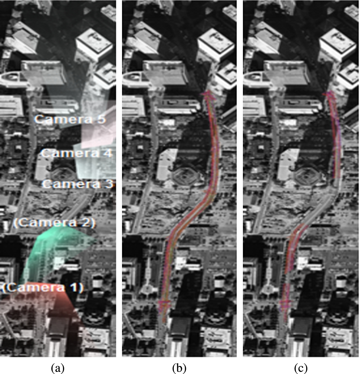

Also, the image plane of the cameras of this dataset are presented in Fig. 4 and the images of two objects in three different poses of dataset NGSIM are shown in Fig. 5.

Fig. 4.

The image plane of the NGSIM dataset: (a) Camera one; (b) Camera two; (c) Camera three; (d) Camera four; and, (e) Camera five.

Fig. 5.

Examples of objects of the NGSIM dataset in different poses: (a) Pose one of object one; (b) Pose two of object one; (c) Pose three of object one; (d) Pose one of object two; (e) Pose two of object two; and, (f) Pose three of object two.

The PETS2009 S2.L1 Walking was captured using eight cameras which is set up to monitor a road corner of a university campus and involves about 10 people. Since the cameras of this dataset have a large amount of overlapping in their coverage only four cameras are used in this paper to reduce the amount of overlapping. The images of two objects in three pose of this dataset are presented in Fig. 8. The world ground plane images of this dataset are presented in Fig. 6 and the image plane of cameras of this dataset are shown in Fig. 7.

Fig. 6.

The world ground plane image of the PETS2009 S2.L1 Walking dataset based on the ground truth annotation: (a) Camera coverage (coverage area of each camera is shown by particular color); (b) Persistent trace (persistent trace of each object is shown by particular color); and, (c) Extracted tracklets (each tracklet is shown by particular color).

Fig. 7.

The image plane of the PETS2009 S2.L1 Walking dataset: (a) Camera one; (b) Camera two; (c) Camera three; and, (d) Camera four.

Fig. 8.

Some examples of objects of the PETS2009 S2.L1 Walking dataset in different poses: (a) Pose one of object one; (b) Pose two of object one; (c) Pose three of object one; (d) Pose one of object two; (e) Pose two of object two; and, (f) Pose three of object two.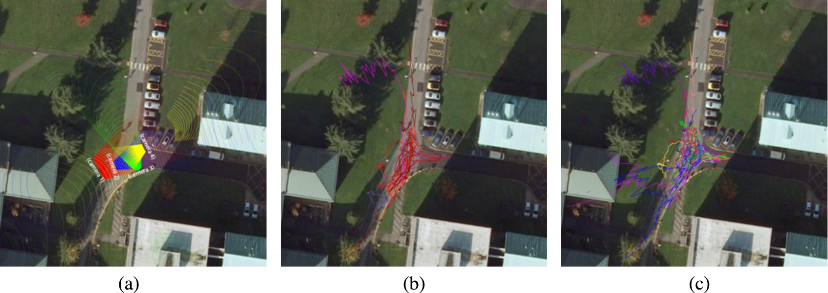

The CAVIAR dataset [7] is collected in a shopping mall corridor with heavy inter-object occlusions. The image size of this dataset are 384 × 288 pixels. The dataset contains two different views of the shopping corridor, the frontal view and the corridor view. But, in our experiment, as has been done in [25], only the corridor view is used. To use the single view of this dataset in our proposed model, at first, tracks of all objects from the ground truth of the corridor view are broken down into the small pieces and the resulted pieces are used as the tracklets in the proposed model. Then, the proposed model is used to associate the small pieces of tracks of objects and determining the overall tracks of each object. In [25] 7 challenging part of the dataset have been used which contains TwoEnterShop3, TwoEnterShop2, ThreePastShop2, ThreePastShop1, TwoEnterShop1, OneShopOneWait1 and OneStopMoveEnter1. The world ground plane images of this dataset are given in Fig. 9. Some examples images of objects of this dataset are presented in Fig. 12. Also, the image plane images of this dataset is shown in Fig. 11. The obtained results of these real datasets are presented in Table 5.

Fig. 9.

The world ground plane top view of the OneStopMoveEnter1 that is part of the CAVIAR dataset based on the ground truth annotation: (a) Camera coverage (coverage area of each camera is shown by particular color); (b) Persistent trace (persistent trace of each object is shown by particular color); and, (c) Extracted tracklets (each tracklet is shown by particular color).

Fig. 10.

The world ground plane image of the synthetic dataset based on the ground truth annotation: (a) Camera coverage (coverage area of each camera is shown by particular color); (b) Persistent trace (persistent trace of each object is shown by particular color); and, (c) Extracted tracklets (each tracklet is shown by particular color).

Fig. 11.

The image plane of the CAVIAR dataset.

Fig. 12.

Some examples of objects from ThreePastShop1 part of the CAVIAR dataset: (a) Pose one of object one; (b) Pose two of object one; (c) Pose three of object one; (d) Pose one of object two; (e) Pose two of object two; and, (f) Pose three of object two.

3.3. Synthetic dataset

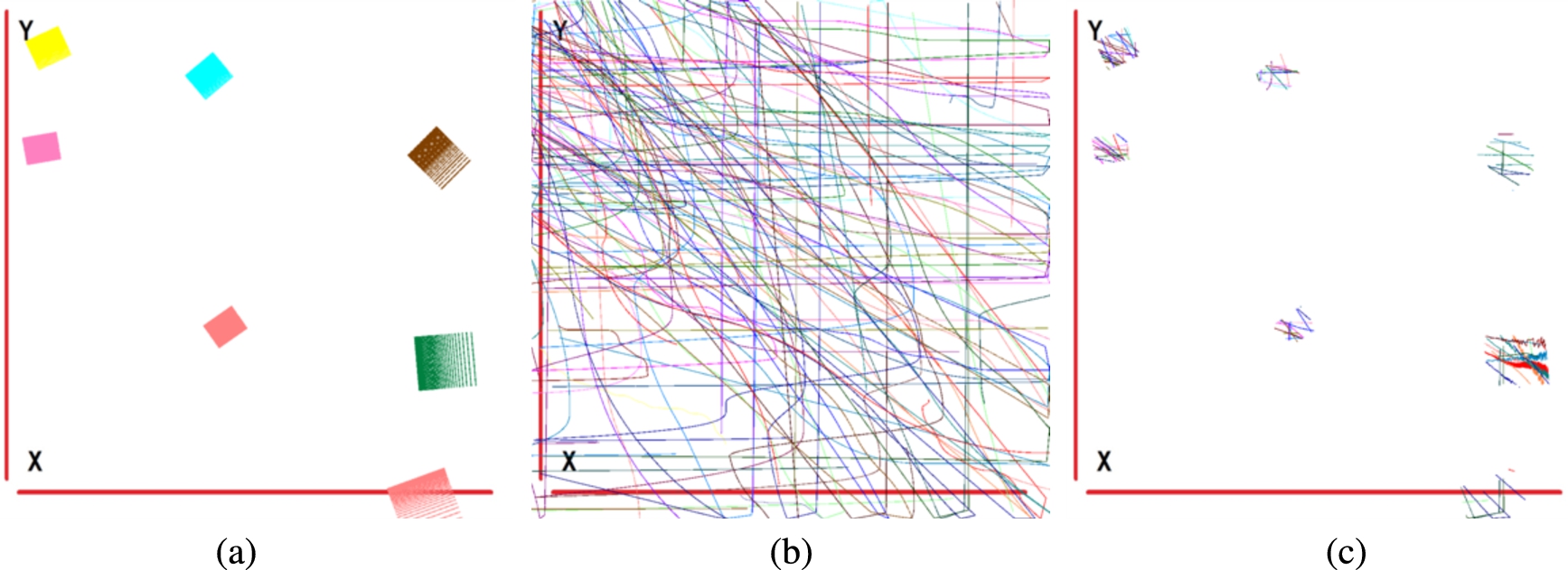
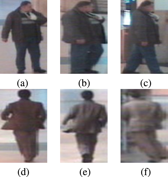
Producing camera network datasets with complicated scenario which embodies the complete annotation are rarely available. Hence, synthesizing the dataset is an alternative for validating our proposed method. A tool has been developed that can generate through annotated dataset according to every complicated surveillance scenario based on the given information [11]. The information includes characteristics of the observed area, parameters and topology of the cameras and the motion and appearance model of the objects. A dataset has been created by this tool. The characteristic of synthetic dataset are presented in Table 3. Also, the world ground plane images of this dataset are shown in Fig. 10. In this tool, the appearance model of the objects can be allotted with real image of the objects. So, in synthetic dataset of this paper, the images of the people in various poses of 3DPeS [3–5] are used as the appearance model of the objects. Some examples of these appearance model are given in Fig. 13. The results of our experiments with this dataset are presented in Table 5.

Fig. 13.

Some examples of objects of the synthetic dataset in different poses: (a) Pose one of object one; (b) Pose two of object one; (c) Pose three of object one; (d) Pose one of object two; (e) Pose two of object two; and, (f) Pose three of object two.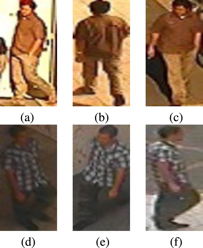

3.4. Results and discussion

In this section, the performance of our proposed model is evaluated and results are compared with two similar studies along with our model. As provided in Table 5, our proposed model can track objects in camera network with the average TCF metric 75.5% and FS metric 74.71% which means it can extract more than 74% of the objects’ persistent trace. Also, the proposed model can track objects with average MT metric of 79.45% which means it can track more than 80% of the persistent trace of more than 79% of the objects. For evaluating our proposed method, the reported results of two other models are used. In [25], a stochastic tracklet association graph is used. Also, they need some information about the topology of cameras and transition models between cameras. In [20] a new space time sheet is proposed and a probabilistic tracking model is used for persistent tracking objects. In addition, they need some high level information such as the lane position of street. However, in our model, we do not need these high level information about the wide area or camera topology. For comparing the results, we used the same metrics as these two models. Based on results shown in Table 5 our proposed method can track objects with less error and closer completeness factor respect to [25]. Also, our proposed method, can track objects more completed traces with less errors with respect to [20]. In other words, the proposed model can present competitive results. Also, the time complexity and the required number of steps for our algorithm which is required for extracting the persistent trace of all objects in four datasets are shown in Table 4.

Table 4
The time complexity and the number of steps required for optimization of the experiments

Datasets	Time Consumption (ms)	Optimized number of steps
CAVIAR	55856	450
NGSIM	177432	975
PETS	15689	551
Synthetic	133137	662

Table 5

The results

Metrics	Our proposed model				B. Song [25] CAVIAR	R. Pless [20] NGSIM

	CAVIAR	NGSIM	PETS2009	synthetic
TCF	71%	74%	74%	83%	–	67%
TF	1.61	1.21	2.0	2.0	–	1.39
POIF	0.37	0.31	0.46	0.33	–	–
PT	83.76%	80.43%	75.35%	87.5%	–	–
ST	72.58%	69.83%	76.14%	77.62%	–	–
FS	75.74%	71.09%	72.43%	79.61%	–	–
IDS	9	28	5	8	8	–
FG	6	35	8	10	6	–
MT	80.1%	73.4%	83.33%	81.0%	84.0%	–
ML	2.0%	12%	0%	0%	4.0%	–

4. Conclusion

In this paper, a novel variational method is introduced for tracking multi-objects in camera networks which imposes less limitative assumptions compare to the previous method in more realistic scenario. The quality and accuracy of the proposed method was evaluated by common metric through experimenting the method on the common real datasets. Also, in order to evaluate the proposed method on a more challenging problem, experiments are performed on the synthetic datasets; tracking problem while requiring less high level information. In order to improve the proposed method, various aspect can be considered. As an alternative, the formulation can be represented such that the persistent trace of all objects can be extracted simultaneously. Further improvement can be achieved by combining our algorithm with high level features, such as human gait recognition.

Footnotes

The appearance and motion formulation

In this appendix the proposed representation for appearance and motion model and distance measure of these models are given. The mean appearance model of object i which is used as a candidate appearance model of this object is defined as, $\begin{array}{l} (21) & F_{A} (ϕ_{i}) = \frac{(\sum_{l = 1}^{| T |} F_{A} (τ_{l}) \times H (ϕ_{i} (l)))}{(\sum_{l = 1}^{| T |} H (ϕ_{i} (l)))}, \end{array}$ and, the mean motion model of object i is defined as, $\begin{array}{l} (22) & F_{M} (ϕ_{i}) = \frac{(\sum_{l = 1}^{| T |} F_{M} (τ_{l}) \times H (ϕ_{i} (l)))}{(\sum_{l = 1}^{| T |} H (ϕ_{i} (l)))} . \end{array}$ Also, mean appearance model of object i without using tracklet $τ_{l}$ is computed as, $\begin{array}{l} (23) & F_{A} (ϕ_{i / τ_{l}}) = \frac{\sum_{j = 1, j \neq l}^{| T |} F_{A} (τ_{j}) \times H (ϕ_{i} (j))}{\sum_{j = 1, j \neq l}^{| T |} H (ϕ_{i} (j))}, \end{array}$ and, mean motion model of object i without using tracklet $τ_{l}$ is defined as, $\begin{array}{l} (24) & F_{M} (ϕ_{i / τ_{l}}) = \frac{\sum_{j = 1, j \neq l}^{| T |} F_{M} (τ_{j}) \times H (ϕ_{i} (j))}{\sum_{j = 1, j \neq l}^{| T |} H (ϕ_{i} (j))} . \end{array}$ Mean distance measure between candidate appearance model of object i and appearance model of each tracklet which exists in the obtained persistent trace of object i is shown as $\begin{array}{rcl} {MeanF}_{A} (ϕ_{i}) \\ (25) & = \frac{(\sum_{l = 1}^{| T |} DistA (F_{A} (τ_{l}), F_{A} (ϕ_{i})) \times H (ϕ_{i} (l)))}{(\sum_{l = 1}^{| T |} H (ϕ_{i} (l)))}, \end{array}$ and mean distance measure between candidate motion model of object i and motion model of each tracklet which exists in the obtained persistent trace of object i is shown as, $\begin{array}{l} {MeanF}_{M} (ϕ_{i}) \\ (26) & = \frac{(\sum_{l = 1}^{| T |} DistM (F_{M} (τ_{l}), F_{M} (ϕ_{i})) \times H (ϕ_{i} (l)))}{(\sum_{l = 1}^{| T |} H (ϕ_{i} (l)))} . \end{array}$ Also, mean distance measure between candidate appearance model of object i and appearance model of each tracklet which exists in the obtained persistent trace of object i without using the tracklet $τ_{l}$ is defined as $\begin{array}{l} {MeanF}_{A} (ϕ_{i / τ_{l}}) \\ (27) & = \frac{(\sum_{j = 1, j \neq l}^{| T |} DistA (F_{A} (τ_{j}), F_{A} (ϕ_{i / τ_{l}})) \times H (ϕ_{i} (j)))}{(\sum_{j = 1, j \neq l}^{| T |} H (ϕ_{i} (j)))}, \end{array}$ and; the mean distance measure between candidate motion model of object i and motion model of each tracklet which exists in the obtained persistent trace of object i without using the tracklet $τ_{l}$ is defined as, $\begin{array}{l} {MeanF}_{M} (ϕ_{i / τ_{l}}) \\ (28) & = \frac{(\sum_{j = 1, j \neq l}^{| T |} DistM (F_{M} (τ_{j}), F_{M} (ϕ_{i / τ_{l}})) \times H (ϕ_{i} (j)))}{(\sum_{j = 1, j \neq l}^{| T |} H (ϕ_{i} (j)))} . \end{array}$

Ill-posed problem

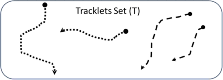
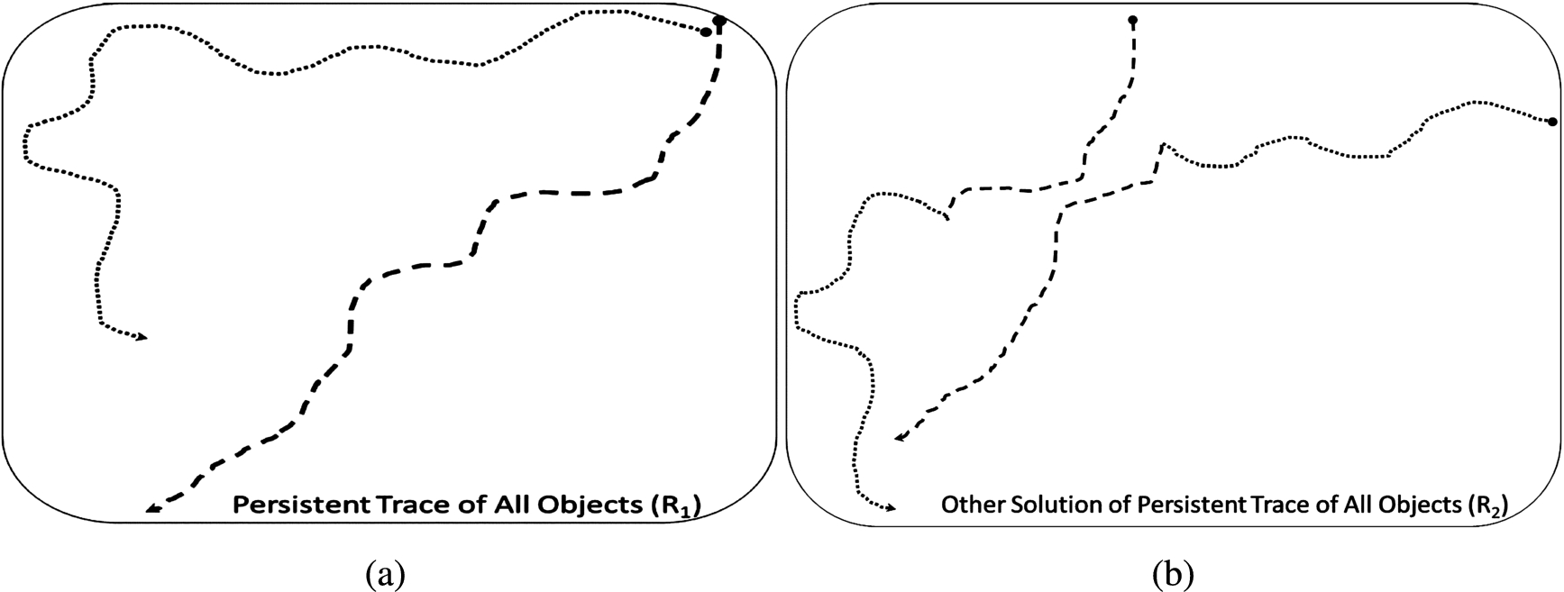
Based on definition of ill-posed problem which is presented in [2] extracting the persistent trace is an ill-posed problem. To prove this claim, we present and analyze a sample of persistent tracking in Fig. 14, the traces of two objects which shown by dots and dash lines representing the movements of these two objects within the wide are ( $n = 2$ ), which is monitored by two cameras ( $k = 2$ ). The movement of these objects in the wide area make four tracklets ( $| T | = 4$ ) as shown in Fig. 15. The objective of the persistent tracking problem is to find the persistent trace of these objects based on the obtained tracklets set T. Therefore, we can model it as an inverse problem as, $\begin{matrix} (29) & T = A R, \end{matrix}$ where T is the tracklets set as an observation of the problem and is known, R is the persistent trace of the objects which is the solution of the problem and is unknown, and A is the sampling function which is performed by the cameras in the wide area. Here, we are to extract the persistent trace R which result in the tracklets set T. If Dash and Dot objects have discriminative models, only one persistent trace set can be found in this problem as shown in Fig. 16(a). But, if they don’t have any discriminative models, more than one solution can be found which are shown in Fig. 16(a) and Fig. 16(b); this kind of problems are known as the ill-posed problems [2]. There are various noise such as pose and illumination variation, occlusion, clutter and sensor noise, which make it almost impossible to find the discriminative model in these problems. Also, extending the under surveillance area, increasing the number of cameras and moving objects make it even more complex to find the favorite models. So, for each input observation more than one solution is possible which make the persistent tracking problem an ill-posed one. Fig. 14.

A sample of the persistent tracking problem.

Fig. 15.

The tracklets set T of the sample presented in Fig. 14.

Fig. 16.

The persistent trace set R of the sample presented in Fig. 14: (a) The first persistent trace set R of the sample, (b) The second persistent trace set R of the sample.

References

[1]

Aghajan and

Cavallaro, Multi-Camera Networks Principles and Applications, Elsevier AP Publishers, Amsterdam, Boston, 2009.

[2]

J.-F.

Aujol, Calculus of variations in image processing, Tech. rep., CMLA, ENS Cachan, CNRS, UniverSud (September 2008).

[3]

Baltieri,

Vezzani and

Cucchiara, 3d body model construction and matching for real time people re-identification, in: Eurographics Italian Chapter Conference, Eurographics,

Puppo,

Brogni and

L.D.

Floriani, eds, 2010, pp. 65–71.

[4]

Baltieri,

Vezzani and

Cucchiara, Sarc3d: A new 3d body model for people tracking and re-identification, in: ICIAP (1),

Maino and

G.L.

Foresti, eds, Lecture Notes in Computer Science, Vol. 6978, Springer, 2011, pp. 197–206.

[5]

Baltieri,

Vezzani and

Cucchiara, 3dpes: 3d people dataset for surveillance and forensics, in: Proc. of the 2011 Joint ACM Workshop on Human Gesture and Behavior Understanding, J-HGBU ’11, ACM, New York, NY, USA, 2011, pp. 59–64. doi:10.1145/2072572.2072590.

[6]

Castanon and

Finn, Multi-target tracklet stitching through network flows, in: 2011 IEEE Aerospace Conference, IEEE, 2011, pp. 1–7. doi:10.1109/AERO.2011.5747436.

[7]CAVIAR, 2009, URL http://groups.inf.ed.ac.uk.

[8]

T.F.

Chan,

Shen, Image Processing and Analysis: Variational, PDE, Wavelet, and Stochastic Methods, Siam, 2005.

[9]

Chan and

Vese, Active contours without edges, IEEE Transactions on Image Processing 10(2) (2001), 266–277. doi:10.1109/83.902291.

10.

[10]Eleventh ieee international workshop PETS, 2009, URL http://www.cvg.reading.ac.uk/PETS2009/a.html.

11.

[11]Image processing & pattern recognition laboratory, URL http://ippr.aut.ac.ir.

12.

[12]

Javed,

Rasheed,

Shafique and

Shah, Tracking across multiple cameras with disjoint views, in: Proc. of Ninth IEEE International Conference on Computer Vision, 2003, Vol. 2, IEEE, 2003, pp. 952–957. doi:10.1109/ICCV.2003.1238451.

13.

[13]

Li,

Huang and

Nevatia, Learning to associate: HybridBoosted multi-target tracker for crowded scene, in: IEEE Conference on Computer Vision and Pattern Recognition, 2009, CVPR 2009, 2009, pp. 2953–2960. doi:10.1109/CVPR.2009.5206735.

14.

[14]

Makris,

Ellis and

Black, Bridging the gaps between cameras, in: Proc. of the 2004 IEEE Computer Society Conference on Computer Vision and Pattern Recognition, 2004, CVPR 2004, Vol. 2, IEEE, 2004, pp. 205–210.

15.

[15]

Micheloni,

Rinner and

Foresti, Video analysis in pan-tilt-zoom camera networks, IEEE, Signal Processing Magazine 27(5) (2010), 78–90. doi:10.1109/MSP.2010.937333.

16.

[16]

K.-J.

Miescke and

Liese, Statistical Decision Theory: Estimation, Testing, and Selection, Springer-Verlag, New York, 2008.

17.

[17]

R.K.

Nagle,

E.B.

Saff and

E.B.

Saff, Fundamentals of Differential Equations and Boundary Value Problems, Pearson Addison-Wesley, 2012.

18.

[18]Ngsim peachtree street, 2007, URL http://www.ops.fhwa.dot.gov/trafficanalysistools/ngsim.htm.

19.

[19]

Paragios,

Chen and

Faugeras, Handbook of Mathematical Models in Computer Vision, Springer, 2006, Printed in the United States of America.

20.

[20]

Pless,

Dixon,

Jacobs,

Baker,

N.L.

Cassimatis,

Brock,

Hartley and

Perzanowski, Persistence and tracking: Putting vehicles and trajectories in context, in: 2009 IEEE Applied Imagery Pattern Recognition Workshop (AIPRW), IEEE, 2009, pp. 1–8. doi:10.1109/AIPR.2009.5466307.

21.

[21]

A.K.

Roy-Chowdhury and

Song, Camera Networks: The Acquisition and Analysis of Videos over Wide Areas, Morgan & Claypool Publishers, 2012. doi:10.2200/S00400ED1V01Y201201COV004.

22.

[22]

Saligrama,

Konrad and

Jodoin, Video anomaly identification, IEEE, Signal Processing Magazine 27(5) (2010), 18–33. doi:10.1109/MSP.2010.937393.

23.

[23]Silogic, Internal technical note metrics definition, Tech. rep., Inria, 2006.

24.

[24]

Song and

A.K.

Roy-Chowdhury, Robust tracking in a camera network: A multi-objective optimization framework, J. Sel. Topics Signal Processing 2(4) (2008), 582–596. doi:10.1109/JSTSP.2008.925992.

25.

[25]

Song and

R.J.

Sethi, Robust wide area tracking in single and multiple views, in: Visual Analysis of Humans,

T.B.

Moeslund,

Sigal,

Krüger and

Hilton, eds, Springer-Verlag, 2011, pp. 1–18 doi:10.1007/978-0-85729-997-0.

26.

[26]

Stauffer and

Tieu, Automated multi-camera planar tracking correspondence modeling, in: Proc. of 2003 IEEE Computer Society Conference on Computer Vision and Pattern Recognition, 2003, Vol. 1, IEEE, 2003, pp. 259–266.

27.

[27]

Unal,

Yezzi,

Soatto and

Slabaugh, A variational approach to problems in calibration of multiple cameras, IEEE Transactions on Pattern Analysis and Machine Intelligence 29(8) (2007), 1322–1338. doi:10.1109/TPAMI.2007.1035.

28.

[28]

C.R.

Vogel, Computational Methods for Inverse Problems, Siam, 2002.

29.

[29]

Wang,

A.G.

Jagola and

Yang, Computational Methods for Applied Inverse Problems, Walter De Gruyter Incorporated, 2012.

30.

[30]

Wang,

Velipasalar and

M.C.

Gursoy, Distributed wide-area multi-object tracking with non-overlapping camera views, Multimedia Tools and Applications (2012), 1–33.

31.

[31]

Z.J.

Xiang,

Chen and

Liu, Feature correspondence in a non-overlapping camera network, Multimedia Tools and Applications (2013), 1–17.

32.

[32]

Yilmaz,

Javed and

Shah, Object tracking: A survey, ACM Computing Surveys (CSUR) 38(4) (2006), 1–45. doi:10.1145/1177352.1177355.

Variational method for wide area surveillance

Abstract

Keywords

1. Introduction

Table 1 Problem notations

2.2. Level set representation

2.3. Numerical solution

3.1. Evaluation metrics

3.2. Real datasets

Table 4 The time complexity and the number of steps required for optimization of the experiments

Footnotes

The appearance and motion formulation

Ill-posed problem

References

Table 1
Problem notations

Table 4
The time complexity and the number of steps required for optimization of the experiments