Benchmarking sensors in smart environments

Abstract

Smart environment applications can be based on a large variety of different sensors that may support the same use case, but have specific advantages or disadvantages. Benchmarking can allow determining the most suitable sensor systems for a given application by calculating a single benchmarking score, based on weighted evaluation of features that are relevant in smart environments. This set of features has to represent the complexity of applications in smart environments. In this work we present a benchmarking model that can calculate a benchmarking score, based on nine selected features that cover aspects of performance, the environment and the pervasiveness of the application. Extensions are presented that normalize the benchmarking score if required and compensate central tendency bias, if necessary. We outline how this model is applied to capacitive proximity sensors that measure properties of conductive objects over a distance. The model is used to identify existing and find potential new application domains for this upcoming technology in smart environments.

Keywords

Benchmark smart environments modeling sensor technology capacitive proximity sensors

1. Introduction

The design of applications and systems involves a number of decisions taken by the developing parties, in order to create an optimized product. Benchmarking is a method that compares the performance of products, market entities or processes against the competition. The first step in this process to select a set of indicators that can be used as a metric to compare the performance of a single factor. Either a single metric or an overall combined metric is used to assess the performance relative to other entities [11]. Benchmarking is widely used as a decision support tool in various domains. The design process for systems in smart environments often involves taking this decision to find a suitable sensor for any given applications. This is often done following a structured approach, e.g. by ranking available technologies or performing iterative development cycles comprised of trial & error. However, there has been no generic model that would allow to estimate the expected performance of an application, given a specific sensor technology. We previously looked at benchmarking as a tool to compare different sensor devices in smart environments, in order to find suitable applications given a specific set of sensors, or find the most suitable sensor for a specific application [8]. This work is an extended edition of this paper. We described how to use a set of common features and an adaptive weighting model, to cover a high number of different applications in a specific domain and thus support the decision process at an early stage of the application design. In this work we root our benchmarking model by providing the real life use case of benchmarking capacitive proximity sensors for a potential set of application domains. This sensing technology has the ability to sense parts of the human body over a distance through any non-conductive material. However, the application in smart environments has been limited so far, compared to technologies, such as cameras. Therefore, it is a suitable candidate to identify potential use cases via benchmarking. Initially we will present related works that are relevant for introducing the benchmarking model and the selection of suitable features. After this, an overview of potential application areas for capacitive proximity sensors is given that builds the basis for further benchmarking performed in Section 7. We will present a discussion and selection of the sensor features and introduce the modal formalism. We provide a proof of the benchmarking concept by performing a popularity analysis of scientific publications. Afterwards, the model is applied to capacitive proximity sensors, in order to identify potential application scenarios.

This work is an extended edition of Braun et al. [8]. It expands from the referenced work and the doctoral dissertation of the corresponding author [6] in the following aspects:

Introduces application domains potentially suited for capacitive proximity sensors.

Provides a more thorough discussion of sensor features for smart environments and provides more examples.

Performs benchmarking for capacitive proximity sensors.

Discusses more explicitly the implications of the benchmarking model and visual analysis methods.

2. Related works

Benchmarking is a tool that is widely used in computing technology [33]. Hardware benchmarks compare the performance of different single systems, often seen for GPUs or CPUs to evaluate both theoretical and real-life performance. Some metrics that are used for theoretical comparison in CPUs are FLOPS (floating point operations per second), e.g. measured by Linpack [19], or MIPS (million instructions per second), e.g. measured by Dhrystone [50]. Regarding GPUs the benchmarks include Texel rate (how many triangles can be processed per second) and Pixel rate (how many pixels are processed per second. Real-life benchmarks for CPUs typically included timing specific tasks on applications that are demanding for certain aspects of the CPU, such as video processing, image processing or audio encoding. For GPUs many PC games provide benchmarking tools that allow evaluating the real-life performance of different graphics cards at different settings, e.g. resolution or detail level. The typical metric here are FPS (frames per second) that denote how often the screen content can be rendered in a second.

System benchmarks are a step up from single component benchmarks and combine the performance measurements of various components in different scenarios to evaluate the estimated behavior in numerous real-life situations. There are several standardized test suites that provide this functionality, such as SPEC [26]. A common single index that is available for all newer Windows machines (Vista and beyond) is the Windows System Assessment tool that calculates the WEI (Windows Experience Index), a combined score of CPU performance, 2D and 3D graphics performance, memory performance and disk performance [52]. The lowest score of all single metrics is the final score and thus determines a lower bound for expected real-life performance.

If different systems of the same category are compared, technology reviewers often use a single index that is calculated based on various aspects of the system. Smith introduced different potential combined metrics that can be used for this purpose [46]. Three different approaches are mentioned, geometric mean, arithmetic mean and harmonic mean. Additionally varieties with a specific weighting are mentioned.

There has been considerable work in the domain of identifying suitable metrics for a given benchmark. Crolotte argued that the only valid benchmark for decision support systems is the arithmetic mean of different single benchmark streams, as it is valid for normalized and time-relevant benchmarks [18]. Jain and Raj dedicate several chapters of their book to introduce methods and considerations for metric selection in benchmarking computer systems [29].

Table 1
Application domains and relevant works

Application Domain Relevant Works

Indoor Localization Braun – CapFloor [7]

Chintalapudi – EZ Indoor localization [13]

Pirkl – resonant magnetic coupling [40]

Gestural interaction Zimmerman – hand gesture [58]

Wilson – XWand pointing interaction [54]

Majewski – Visual feedback [35]

Pu – WiSee [42]

Physiological sensing Cowie – emotion recognition [16]

Khosrowabadi – EEG emotion [30]

Hoque – MACH [27]

Activity recognition Bao – user-annotated acceleration data [2]

Bulling – electrooculography [10]

Oreifej – Hon4D [39]

Smart appliances Gellersen – MediaCup [21]

Yeo – StickEar [57]

Tsai – Smart Medication Dispenser [48]

Mobile devices Ballages – mobile devices in ubiquitous computing [1]

Nazari Shirehjini – PECo [45]

Olsson – mobile augmented reality [38]

Autonomous systems Coradeschi – symbiotic robotic systems [15]

Glas – social robots in smart homes [22]

Application Domain	Relevant Works
Indoor Localization	Braun – CapFloor [7]
Chintalapudi – EZ Indoor localization [13]
Pirkl – resonant magnetic coupling [40]
Gestural interaction	Zimmerman – hand gesture [58]
Wilson – XWand pointing interaction [54]
Majewski – Visual feedback [35]
Pu – WiSee [42]
Physiological sensing	Cowie – emotion recognition [16]
Khosrowabadi – EEG emotion [30]
Hoque – MACH [27]
Activity recognition	Bao – user-annotated acceleration data [2]
Bulling – electrooculography [10]
Oreifej – Hon4D [39]
Smart appliances	Gellersen – MediaCup [21]
Yeo – StickEar [57]
Tsai – Smart Medication Dispenser [48]
Mobile devices	Ballages – mobile devices in ubiquitous computing [1]
Nazari Shirehjini – PECo [45]
Olsson – mobile augmented reality [38]
Autonomous systems	Coradeschi – symbiotic robotic systems [15]
Glas – social robots in smart homes [22]

In smart environments a number of different benchmarks have been proposed that cover aspects similar to our approach. Ranganathan et al. introduced benchmarking methods and a set for pervasive computing systems [43]. They distinguish system metrics, configurability and programmability metrics and human usability metrics. Another example for benchmarking whole systems is the EvAAL competition that aims at evaluating different technologies that are applicable in Ambient Assisted Living [4]. There are various tracks, including indoor localization and activity recognition. Apart from technical metrics, such as precision, a focus of this competition is on a more holistic approach and thus includes metrics like installation time, user acceptance and interoperability of the solution. Santos et al. presented a model to evaluate human-computer interaction in ubiquitous computing applications, based on trustability, resource-limitedness, usability and ubiquity [44]. In order to assess how well ubiquitous computing applications cover privacy aspects, Jafari et al. propose a set of five abstracted metrics that are applied to whole systems [28]. While these are all benchmarking models within smart environments, they are either aiming at evaluating whole systems or singular aspects not directly related towards sensor technology.

3. Smart environments applications for capacitive proximity sensors

The field of smart environments is not strictly and conclusively distinguished from other fields in technology. It is using influences from disciplines including electric engineering, behavioral psychology, computer science, or mechanical engineering. Accordingly, it is difficult to formally list or distinguish all applications that are relevant or have been tackled in previous work. As indicated in the introduction, in this work we are focusing on a subset of potential application domains that may be suitable for capacitive proximity sensors. The chosen applications are taken from different collections of work that have been released in the past few years. Cook et al. that presented a survey on recent developments in smart environments research in 2007 [14]. Augusto et al. edited a book on ambient intelligence in 2009, including chapters on various domains and applications [37]. Another source is the book Ubiquitous Computing by Poslad, released in 2011 [41]. Additionally, we took into account recent conferences and journals that are active in this regard, such as CHI or UbiComp.

Capacitive proximity sensors use variations in electric fields to gather information about conductive objects in detection range. A common variety is the mutual capacitance touch screen that enables the sensing of multiple fingers on today’s smart phones and tablets [3]. The proximity sensing versions uses larger electrodes and different sensing methods to detect objects over a distance. There is a large number of potential applications for this type of technology. An overview can be found in this previous work by our group [9]. This allows us to refine the potential application domains to a more manageable count. By linking the general overview and applications for capacitive proximity sensors a set of seven candidate application domains can be selected. They are outlined in Table 1. On the following pages we will briefly introduce relevant work in those domains.

3.1. Indoor localization

The reliable tracking and localization of multiple users is a major challenge in smart environments. It is a very important contextual information that can be used to adapt the behavior of the environment. Often basic motion sensors are used, e.g. if just a single person should be detected or if there is a single area of interest that should be covered. However, determining a more exact location or following multiple users requires more sophisticated systems. If a varying number of non-relevant actors are moving in the environment, e.g. pets, the challenge is additionally increased. One example system that was developed by our group is CapFloor – that uses capacitive proximity sensors and a grid layout for electrodes, in order to detect location and falls of users within detection range [7].

A common method is to use radiofrequency sensing, tracking a mobile token, e.g. based on 802.11 WiFi networks. A recent work in this domain has been presented by Chintalapudi et al. [13]. Their EZ system relies on an existing WiFi infrastructure, the user carrying a mobile device with WiFi that also has periodic access to a GPS signal. It does not require any prior mapping or knowledge about the specific location or transmit power of the access points, but instead relies on a genetic algorithms to determine potential locations from a limited set of known locations and distances to access points calculated using the received signal strength (RSSI).

A final example is a system created by Pirkl and Lukowicz based on resonant magnetic coupling [40]. Using the magnetic field created by static coils, an arbitrary number of mobile receivers can localize themselves by measuring the field strength and estimating the distance from the different static coils. The system can be calibrated to ignore other magnetic objects in vicinity and enables a planar localization of about 1 m² accuracy.

3.2. Gestural interaction

Gesture recognition enables the detection of meaningful expressions of motion by a human body, including the hands, arms, face, head and body [36]. If these expressions are translated into machine commands the result is gestural interaction. The most expressive and explicit form of gestures are performed by the hands, further distinguished into free-air gestures and touch gestures that typically involve one or more fingers interacting with a surface. The second variety is called multi-touch.

Throughout the years there have been various attempts to enable the tracking of gestures in free air. A common attempt in the late 1980s were data gloves, sensor-augmented gloves put on the hand that translated finger movements to gestural input, e.g. the system presented by Zimmerman [58]. It uses optical sensors to measure the flex of the fingers and ultrasonic sensors to detect the absolute position and orientation of the hand. Applications included the evaluation of hand impairments and object manipulations in three-dimensional scenes.

A different approach is performing gestural interaction supported by interaction devices that can sense orientation and position in the room. A popular example is the Nintendo Wii Remote that is used in gaming applications.

A predecessor was the XWand by Wilson et al. [54]. This interaction device is using accelerometers to sense orientation and has infrared diodes that are tracked by an external camera system to determine the absolute position in the room. Using knowledge about the location of different appliances within this room, it is possible to control them by pointing in this direction. Later extensions include a pointing device based on a laser that indicates the position in the environment currently pointed at. This can be realized using the skeleton tracking of a Kinect sensor [35].

WiSee presented by Pu et al. [42] is using two sources of wireless signals, they are using the Doppler shift caused by the human body moving in the area and reflecting the signal to determine gestures. The system was able to detect nine different full-body gestures with a precision of 94%. The system uses the multiple-input and multiple-output (MIMO) capabilities of modern WiFi systems to distinguish users and providing the option to support multiple users within an environment.

3.3. Physiological sensing

In the 1990s researchers began to distinguish different channels when interacting with machines. The explicit channel, whereas the user gives distinct commands to the user, and the implicit channel that comprises information about the user himself [16]. One interesting parameter to consider for this implicit interaction is emotion. Based on physiological cues it is possible to determine the current state of the user and translate it to an input for machines. Thus, an area has emerged that uses acquired physiological signals of the users to provide additional input.

Khosrowabadi et al. presented a machine learning approach to discriminate four different emotions from EEG readings [30]. The subjects were asked to fill out self-assessment questionnaires regarding their emotional state with the states being induced by a set of pictures. The signals were classified using a self-organizing map and nearest-neighbor classification. The system was able to correctly classify 84.5% of four different emotional states.

An example application for emotion-aware systems has been presented by Hoque et al. [27]. MACH: My Automated Conversation coacH is a training system that tries to improve the social skills of its users. It collects facial expressions, speech data and analysis prosody from an attached camera to create a personalized feedback of the user’s behavior when talking to a virtual agent. A study with 90 participants showed a significant performance improvement as opposed to the control group. In this domain it is also very important to build databases of labeled emotions and physiological signals that allows other researchers to try new methods.

3.4. Activity recognition

Activity recognition, also called situation awareness, describes the interpretation of sensor data into higher domain-level information that relates to the given situation [56]. To give an example, a single temperature reading of $15^{\circ} C$ can be combined with the information that the sensor is in the sleeping room, the time is 21:00 and we know that the inhabitant of the environment is typically going to sleep at 22:00. In this case we can infer the activity user will go to bed soon and trigger the action heat up sleeping room. There is a plethora of different concepts and methods on how to recognize the situations and activities for numerous domains.

When trying to determine human activities wearable sensors are an important approach that has been used extensively. It is possible to use either physiological measurements or movement data. A classic work in this domain presented by Bao et al. is associating activities based on movement data generated by accelerometers [2]. This sensor category is able to detect the acceleration in multiple directions, e.g. commonly used to detect the orientation of mobile devices. Using five different sensors attached to arms, legs and hip, they were able to associate 20 different activities performed by 20 different subjects with an accuracy of approximately 80%.

In some application domains that have a specific set of tasks other approaches might be suitable. An interesting system was presented by Bulling et al. that tries to determine activities based on the movement of the eyes [10]. They are attaching a set of electrodes to the user’s head to track the activity of muscles around the eye, without using any external sensors such as gaze trackers. In a study with eight users they tried to distinguish five different typical office work activities using SVM classification. These activities are copying text between documents in a two monitor setup, reading a document on the table, writing on a page on the table, watching a video and browsing the internet. The achieved average precision was 76% and recall 71%.

A final example in the domain of activity recognition is Hon4D, a system that infers situation from depth camera sequences [39]. They suggest the histogram of normal orientation in depth, time and spatial coordinates as a feature for activities from depth data. The advantage of this operator is that it takes into account the movement of the overall surface of recognized persons, as opposed to silhouettes or the reconstructed skeleton joints. This approach reaches classification precision between 89% and 97% when used on common activity depth data sets.

3.5. Smart appliances

Smart appliances are devices that are attentive to their environment. This is usually achieved by integrating different sensors and actuators to provide additional functions and services to a user. Some examples include intelligent furniture that can detect their occupation, internet-connected household items, or single-purpose devices, e.g. providing reminder services.

One example for common household items augmented with additional features is the MediaCup by Gellersen et al. [21]. This coffee cup is augmented with temperature and acceleration sensors, a processing unit and communication using an infrared system. It is able to sense if there is fresh coffee in the cup, if it currently used for drinking, stationary or being played with. The applications were focused on remote colleague awareness, whereas the activities of the MediaCup were transmitted to a remote location.

StickEar by Yeo et al. is a wireless device that adds different capabilities to objects it is attached to [57]. They integrate a rotary switch, buttons, microphone, speaker and processing and communication components into a small portable package. Some supported interactions are control of devices using sound, autonomous response to sound events, or remote triggering of sound. The system can be controlled using an app for mobile devices.

There is a number of smart appliances in the medical domain. They try to provide different services related to health and well-being. A common example are smart medication dispensers, such as the one presented by Tsai et al. [48]. Based on a medication schedule it will dispense the right medication and dose at the specified times. They include a few different algorithms for heuristic scheduling based on a collaborative approach between scheduler and the controller of the dispenser.

3.6. Mobile devices

The prevalent smart phones and tablets nowadays resemble closely the smart tab, envisioned by Weiser – handheld devices that provide sensing, interaction and communication facilities supported by sufficient processing power [51]. Consequently, they are used very often in smart environment applications.

Ballages et al. collected and investigated numerous ways how smart phones can be used to in ubiquitous computing [1]. They provided an overview of different positioning, orientation and selection methods, including using the camera on the mobile phone and different processing methods to control a cursor. An important contribution was a classification of potential mobile phone interactions and a summary of position, orientation and selection techniques.

Nazari Shirejini presented PECo, an environment controller based on a PDA device [45]. Based on a 3D model of the current environment it was possible to control different appliances by selecting them on the mobile device. Additionally, a concept was presented that allows to transfer documents from the PDA to different suitable devices, by using simple drag & drop operations. The practical use case was implemented in a lecture room and connected to the controlling system, e.g. allowing to display documents on a projector by dropping them on the 3D model of the projecting screen.

A final example is in the popular domain of augmented reality systems for mobile devices. There are numerous popular applications that overlay additional information on a live camera image of mobile phones. Olsson et al. tried to evaluate user experience and acceptance of different mobile augmented reality applications [38].

They found that information applications were better received than entertainment applications. In addition, information flood, loss of autonomy and virtual replacement of actual items were seen as most negative aspects of this technology.

3.7. Autonomous systems

Autonomous systems are an important future application in smart environments. While factory complexes started using robots decades ago, the trend towards home robotics is fairly recent, as the processing and sensing capabilities of the systems increased, while the price could be reduced significantly. There are numerous potential use cases, ranging from vacuuming or gardening robots, to full-service robots that can be used in care systems for the elderly.

Coradschi and Saffiotti propagated the symbiotic properties of robots operating in a smart environment [15]. Human, robot and smart environment are modeled as three distinct actors that share resources and information between each other. The distributed systems in the environment, e.g. sensors, tags and actuators, can deliver additional information to the control unit of the autonomous system that can be used to optimize any strategies. Similarly, users can benefit from the coordination between robot and environment to achieve common goals.

Glas et al. investigated how robots can track people and localize themselves in social environments that are frequented by a larger number of persons [22]. They combine laser range-scanners placed in the environment that provide wide coverage and are able to track the trajectories of moving persons and robots. This is combined using Kalman filtering with the odometry data generated by the robots. As a combined solution this enables localization of both people and robots in a shared global coordinate system. One example application system uses robots to provide directional information to shoppers in a mall.

4. Sensor features

One of the most challenging aspects of benchmarking is selecting the appropriate metrics to be included. In order to identify relevant sensor features for technologies to be applied in smart environments we take inspiration from sensor technology overviews [53] and the pervasive model presented by Ranganathan et al. [43]. Ye et al. provided an overview of semantic web technologies used in pervasive computing. They analysed existing approaches and provided a roadmap on using the Semantic Web as a platform for sensor-centric systems [20].

4.1. Selecting feature categories

We would like to begin this section by stating that any selection of features and categories is bound to lead to discussions regarding the importance of selected features and the disregard for certain other ideas. Inspiration from previous work and own experience is the most important aspect that drives us in the selection process. In the following we list different rules that were applied in the feature selection:

Features should not rely on dynamic aspects that can be optimized during manufacturing.

Ability to and precision of detecting physical characteristics are important.

Networked sensing devices might become ubiquitously applied in environments.

Balance is required in covering most important aspects and keeping benchmarking manageable.

Categories should be equally represented concerning feature count.

Dynamic aspects, including price or energy consumption are very important when designing actual products and have to be considered early on in the process. However, they often change with scale of the developed system and actual application. E.g. the camera systems deployed in modern smartphones would have been barely affordable in a precision research instruments merely a decade ago. As we are concerned with prototypical applications that may not see a market entry for several years the prerequisites and capabilities of manufacturing may have changed in the meantime. An aspect that is not (critically) changing over time is the ability and precision of capturing different physical characteristics. This precision applies to both spatial and temporal domains and should be reflected in potential categorization.

In recent years the trend is increasingly towards growing connectivity of devices with projections expecting several billion internet-connected devices during the next decades. These can eventually integrate seemingly into the environment and thus unobtrusively provide data generation. This should be reflected in the selection of categories of features.

Another important aspect is that the overall model still has to be manageable. The overall number of categories should not be too high, while at the same time contain a sufficient number of features to capture the complexity in the category. Potentially, this could be adapted in the future to provide multi-layered benchmarking tools, whereas generic benchmarks covering a limited number of categories are applied before more detailed categorical benchmarks. Finally, the number of features within one category should be similar, to ensure an equal representation during the scoring process. This prevents unequal weighting of categories early in the benchmarking process. In the later stage this might be differentiated by individual feature weights, if so desired.

Therefore, we are settling on a number of three for the feature categories: sensor performance characteristics, pervasive metrics and environmental characteristics. These different groups are detailed in the following sections. We are giving an overview of different potential features of the categories, discuss their relevancy for the benchmarking model and create a feature matrix, as a basis for the feature scoring model.

4.2. Sensor performance characteristics

This group of sensor features is related to specific technical properties of the given sensing device, as they would be typically put into the datasheet. A first important characteristic is the sensitivity or resolution of a sensor, which is the smallest change of a measured quantity that is still detectable. For example an accelerometer might be able to only detect changes that are above 0.1 g. Another important characteristic is the update rate of a sensor. This denotes the number of samples the sensor is able to measure in a certain timeframe. Typically, the number of samples in a second is noted as frequency, thus a sensor may have an update rate of 20 Hz, generating 20 samples in a second. Another factor that is particularly important for embedded systems or wearables is the power consumption of the sensor that may limit the time it can operate on battery, independent of a power source. A last example is the detection range, denoting the maximum distance between the measured object and the sensing device. This can be a significant distance for cameras (e.g. satellite images), whereas we are primarily looking at smaller smart environments, where it is rare that distances of 20 meters are exceeded. Other technologies such as capacitive proximity sensors may not work at this distance [9].

4.3. Pervasive metrics

Pervasive metrics can be identified as features that specify how well a given sensor system will perform in collaboration with smart environments, when networked with other devices and when placed into existing surroundings. An example for the latter is the obtrusiveness of a sensor device. If it is clearly visible when applied, if there are disturbing signals generated, or if certain privacy concerns are associated to the sensor device, the acceptance by the user and thus the applicability is reduced. If the sensor is operating in a larger network of other devices, the bandwidth required to submit signal to an analyzing node should be kept low. Equally, if the processing capabilities are limited, less complex data processing is preferable. The overall system cost is increasing if single sensors are particularly expensive, thus limiting the potential applications. The system and attached sensors should be robust, both in terms of physical design and quality of service. Finally, the sensors are more readily applicable if the systems are interoperable to each other.

4.4. Environmental characteristics

The third group is the environmental characteristics of a sensor system. Any sensor is affected by a certain disturbance caused by factors in the environment that are similar to the measured quantity, also called noise. For example an optical sensor is influenced by ambient light sources. In this context it is relevant how frequent those influences are in a certain environment and how robust the sensor is against noise. In many cases the presence of noise can be detected and counteracted with a calibration towards the changed environmental factors. The complexity of this calibration is another interesting factor in this regard. Finally, all sensors have some unique limitations, e.g. specific materials that absorb certain wavelengths of the electromagnetic field are difficult to detect for sensors that work in this specific frequency range.

4.5. Discussion of feature selection

We want to select the three most relevant features of each category. This allows for a more manageable overall model, however, requires a selection of the presented features. In this work the selection is based on the authors’ analysis of the related works. In future it is advisable to use more sophisticated methods, such as surveying AmI experts and calculating inter-rater reliability [31]. Of the sensor performance characteristics group we will select resolution, update rate and detection range. Resolution is a critical feature in any application. It determines how precise any detection is performed and thus, if any particular objects may be detected at all. Update rate is equally important if fast objects are to be detected and if we want to have reactive systems that respond in real-time. The importance of detection range correlates with the size of the environment and may lead to a reduction of required sensors. Of the mentioned features we omit power consumption. The actual power consumption of a whole system is a more interesting metric but very difficult to predict from the energy usage of a single sensor [5].

Table 2
Feature matrix denoting capabilities required for a certain rating

Feature -- - o + ++

Resolution (res) very coarse coarse normal fine very fine

Update Rate (upd) <once per second slower real-time real-time faster real-time >100 times per second

Detection Range (det) touch less than one meter less than 5 meters less than 20 meters more than 20 meters

Unobtrusiveness (unob) open large system open small system hidden, large exposure hidden, noticeable exposure invisible

Processing Complexity (proc) single sensor CPU 10+ sensors CPU single sensor embedded chip 10+ sensors by single chip no further processing

Robustness (robu) single point of failure error detection quality of service self-recovery fully redundant

Disturbance Frequency (disfr) very frequent frequent average unlikely highly unlikely

Calibration Complexity (calco) very hard hard normal easy very easy

Unique Limitations (uniql) very critical critical average not critical none

Feature	--	-	o	+	++
Resolution (res)	very coarse	coarse	normal	fine	very fine
Update Rate (upd)	<once per second	slower real-time	real-time	faster real-time	>100 times per second
Detection Range (det)	touch	less than one meter	less than 5 meters	less than 20 meters	more than 20 meters
Unobtrusiveness (unob)	open large system	open small system	hidden, large exposure	hidden, noticeable exposure	invisible
Processing Complexity (proc)	single sensor CPU	10+ sensors CPU	single sensor embedded chip	10+ sensors by single chip	no further processing
Robustness (robu)	single point of failure	error detection	quality of service	self-recovery	fully redundant
Disturbance Frequency (disfr)	very frequent	frequent	average	unlikely	highly unlikely
Calibration Complexity (calco)	very hard	hard	normal	easy	very easy
Unique Limitations (uniql)	very critical	critical	average	not critical	none

Of the pervasive metrics group we select unobtrusiveness, processing complexity and robustness. Unobtrusiveness of the sensor device is a desired feature in many different scenarios, where it should not impede the environment.

While microprocessors are becoming ever faster, processing complexity is still crucial if the number of sensors is increasing. A dedicated chip will require a more complex architecture and lead to more cost, higher energy usage and more potential points of failure, leading to the final chosen feature of robustness, both against physical abuse, but also in terms of system design, where it should be resilient towards failure of single components. We omitted the required bandwidth, as this metric is not important for many sensors, as they have low bandwidth requirements in general, but also the available bandwidth in wired and wireless systems is increasing continuously. In the last group of environmental characteristics we choose frequency of the disturbing factor, calibration complexity and unique limitations. If the disturbing factor occurs only rarely, it is not critical and therefore, should be part of the benchmark. Calibration complexity combines both the processing complexity and time that is required to recalibrate the system. This is highly important in real-time systems that have to monitor the environment continuously. Finally, unique limitations are a rather broad metric that is difficult to quantify. However, in many scenarios it is obvious that a specific limitation might arise, e.g. if the smart environment is in an area with a lot of human noise, microphones could be regularly disturbed. Including this metric allows modeling those applications into the benchmark with a strong weight penalizing unsuited sensors.

4.6. Feature matrix

From the selected metrics we want to create a feature matrix that allows us to associate specific capabilities to a specific rating that is used later in the scoring process of the benchmark model. Each feature is mapped to five different ratings on an ordinal rating scale comprised of the items “least favorable” (--), “not favorable” (-), “average” (o), “favorable” (+) and “very favorable” (++). This leads to the feature matrix shown in Table 2, which will be discussed briefly.

Resolution is ranging from “very coarse” to “very fine”. We are using this unspecific rating, as the range may vary strongly between different sensor types. A mapping to actual should depend on the application and object that has to be detected. If the object is large, a sensor that would be ranked “coarse” for smaller objects can be ranked as “fine”. One example is an accelerometer with a smallest detectable increment in resolution of $a_{\min} = 0.01 m / s^{2}$ versus another who detects increments of $a_{\min} = 0.1 m / s^{2}$ .

Update Rate is rated around real-time performance that is often rated at around 20 samples per second. Slower sensors might miss various events, while faster sensors allow detecting highly dynamic events. It should be noted that for certain sensor categories that measure fast events can require considerably faster update rates. Coming back to the accelerometer example, the first can provide measurements 10 times per second, while the second accelerometer can provide new measurements 100 times per second.

Detection Range is rated around the 5 m distance mark, that is typically enough to cover the entirety of a single apartment room. For larger rooms sensors with a higher detection distance are favorable, many sensors only react to touch.

Unobtrusiveness is ranging from exposed systems placed in the environment (one example would be the Microsoft Kinect) to invisible systems that integrate seamlessly into the environment.

Processing Complexity has a range from dedicated CPUs that are required to process the data of a single sensor to smart sensors that require no further processing, which allows to apply numerous sensors without adding additional processing capabilities to the environment.

Robustness is following criteria for quality of service. The least favorable system fails, if only a single node is present and failing. The preferred system is fully redundant.

Disturbance Frequency is ranging from frequently occurring disturbing signals, to highly unlikely disturbing signals, resulting in a better rating.

Calibration Complexity is a combined metric including the calibration time, the required processing capabilities and if external aid is required in the calibration process, leading to a rating from “very hard” to “very easy”.

Unique Limitations should be ranked according to their criticality, as previously explained they may be suitable to penalize certain sensors or emphasize the prevalence of a disturbing factor in a noisy environment.

Now that the feature matrix is complete, the next step is presenting the formalized benchmarking model and how we can use the presented features and their rating to calculate a benchmark score that allows us to compare different sensor categories with regard to different applications.

5. Benchmarking model

Fig. 1.

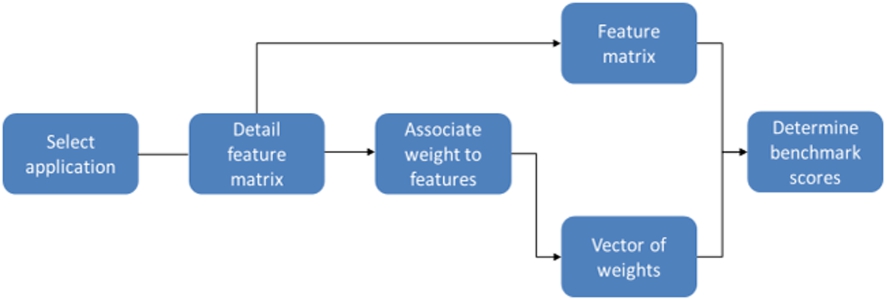
Benchmarking process.

In this section we will describe a formal model that will allow us to determine a benchmark score for a given application and a given sensor technology. As previously explained, the applications are distinguished by applying a different set of weights to the known features. We will begin by discussing the process of this feature weighting and giving some examples about proper application. Afterwards, we will introduce a formal model that deduces a single score benchmark for any sensor technology and any application. The overall process is shown in Fig. 1 and will be detailed in the following sections, including an example.

5.1. Feature score and weighting

The presented feature matrix has some ratings that need detailing in order to be quantifiable in the specific application. The ordinal measurements of the feature matrix should be assigned a quantifiable measure. Taking “Unobtrusiveness” the open system can be detailed as “visible by users” and “large system” as size larger than $100 \times 100 \times 100 mm$ . Similar levels of detail can be applied to the other features, leading to the application-specific detailed feature matrix that is used in the scoring process. The different ratings are assigned different numeric values, namely 0.00 (--), 0.25 (-), 0.5 (o), 0.75 (+) and 1.00 (++). The weight of the features for the specific application is also rated on a 5-point ordinal scale, denoted as “not important” (numeric value 0.0), “less important” (0.25), “moderately important” (0.5), “important” (0.75) and “very important” (1.00). Thus for each application we have a distinct detailed feature matrix and a vector of associated weights that can be applied to a set of sensor technologies in order to calculate the benchmark score. We will now introduce the formal modeling that allows us to determine the calculation for this scoring process.

5.2. Modeling

The model is supposed to formalize a benchmark for any application and any sensor technology in any domain. We will start with the following definitions:

Set of n domains $D = {d_{1}, \dots, d_{i}, \dots d_{n}}$ .

Set of m applications $A = {a_{1}, \dots, a_{j}, \dots a_{m}}$ .

Set of o features $F = {f_{1}, \dots, f_{k}, \dots f_{o}}$ .

Set of p sensor technologies $S = {s_{1}, \dots, s_{l}, \dots, s_{p}}$ .

In any domain $d_{i}$ we have a set of potential applications $A_{d_{i}} \subseteq A$ and a set of relevant features $F_{d_{i}} \subseteq F$ . For each feature $f_{k, d_{i}}$ there is the associated feature score $r_{F_{d_{i}}}$ as explained in the previous section. Each sensor technology $s_{l}$ has a specific feature score $r_{s_{l}, F_{d_{i}}} \in [0, 1]$ . The combined feature scores result in the following vector in Eq. (1). $\begin{matrix} (1) & \overset{⇀}{r_{s_{l}, F_{d_{i}}}} = (\begin{matrix} r_{s_{l}, f_{1, d_{i}}} \\ ⋮ \\ r_{s_{l}, f_{o, d_{i}}} \end{matrix}) \end{matrix}$

The weights $w_{f_{o}} \in [0, 1]$ associated to a specific application $a_{j}$ in a domain $d_{i}$ have the same cardinality $| w |$ as the vector of feature scores $| \overset{⇀}{r_{s_{l}, F_{d_{i}}}} |$ , leading to Eq. (2). $\begin{matrix} (2) & \overset{⇀}{w_{a_{j}}} = (\begin{matrix} w_{f_{1}, a_{j}} \\ ⋮ \\ w_{f_{o}, a_{j}} \end{matrix}) \end{matrix}$

The feature scores and associated weights allow us to determine a benchmark score $b_{s_{l}}$ for a specific sensor technology $s_{l}$ for any application $a_{j}$ by using the scalar product of feature score and respective weight and apply normalization with regard to the weight, as shown in Eq. (3). $\begin{matrix} (3) & b_{s_{l}} = \frac{\overset{⇀}{r_{s_{l}, F_{d_{i}}}} \cdot \overset{⇀}{w_{a_{j}}}}{\sum_{k = 1}^{o} w_{f_{k}, a_{j}}} \end{matrix}$

We can now compare different sensor technologies by calculating and comparing the different benchmark scores for a given set of sensor technologies $S_{p} \subseteq S$ and receive a set $B_{S_{p}}$ with $t = | S_{p} |$ , resulting in Eq. (4). $\begin{matrix} (4) & B_{S_{p}} = {b_{s_{l}, 1}, \dots, b_{s_{l}, t}} \end{matrix}$

Thus in order to determine the optimal (chosen) sensor technology $b_{c}$ for an application $a_{j}$ and given the prerequisites regarding non-negativity of weights and feature scores, we can evaluate the set for the maximum element in Eq. (5). $\begin{matrix} (5) & b_{c} = max (B_{S_{p}}) \end{matrix}$

5.3. Feature score normalization

With regards to actual benchmarking the problem of bias towards a specific technology may occur. If the average features ratings are different between two technologies the calculated benchmark score will increase. In many instances this might be beneficial, yet if comparing numerous technologies to a set of different applications a trend might be more important than absolute scores. Thus, we provide an optional step of calculating the normalized feature vector $r_{s_{l}, F_{d_{i}}, norm}$ with regard to the average associated value of 0.5, using the following Eq. (6). $\begin{matrix} (6) & \overset{⇀}{r_{s_{l}, F_{d_{i}}, norm}} = (\begin{matrix} r_{s_{l}, f_{1, d_{i}}} \\ ⋮ \\ r_{s_{l}, f_{o, d_{i}}} \end{matrix}) \cdot \frac{o \cdot 0.5}{\sum_{p = 1}^{o} r_{s_{l}, f_{p, d_{i}}}} \end{matrix}$

The feature-normalized benchmark score is accordingly determined with the following Eq. (7). $\begin{matrix} (7) & b_{s_{l}, norm} = \frac{\overset{⇀}{r_{s_{l}, F_{d_{i}}, norm}} \cdot \overset{⇀}{w_{a_{j}}}}{\sum_{k = 1}^{o} w_{f_{k}, a_{j}}} \end{matrix}$

5.4. Benchmark scoring

Now with the formal model and the available set of feature matrix and weights we are able to calculate the benchmarking score for a set of sensor technologies. As an example we are choosing the application indoor localization in a public shopping area to monitor customer behavior. As a first step the feature matrix has to be detailed according to the specific requirements of the application. These include a tracking accuracy of 50 cm, with a large area to cover and potentially fast moving persons. Thus the importance ratings for performance characteristics are moderately important for resolution, important for update rate and very important for detection range. The system can also be used for security purposes, thus unobtrusiveness is less important. There can be dedicated servers, so processing complexity is not important, but the system should be difficult to disturb, thus robustness is important. Disturbance frequency is moderately important, as a large number of persons is monitored, leading to statistically significant results, even if single measurements are disturbed. The environment is fairly static, thus calibration complexity is less important. It is possible that a crowded shop produces a lot of acoustic noise, therefore no unique limitations towards acoustic disturbances should be present and this is moderately important. The resulting vector of weights is shown in Eq. (8). $\begin{array}{l} (8) & \overset{⇀}{w_{a}} = {(0.50 0.75 1.00 0.25 0.00 0.75 0.50 0.25 0.50)}^{T} \end{array}$

This vector of weights is static for the benchmarking of this specific application. As a next step it is necessary to determine the feature scores for a sensor technology. In this case, we assume a selection based on previous experiences and best practice for this application and choose a system based on numerous stationary cameras. The system has high resolution cameras, with an update rate of 30 samples per second and a high detection range of more than 20 meters. The cameras are external, not hidden from view but attached on the ceiling. The processing complexity is very high, requiring a dedicated CPU per camera. Since they are out of reach they are robust towards human intervention and independent from each other. In the given setting visual disturbance is unlikely, calibration is difficult but not required regularly and the system is not disturbed by acoustic noise. This results in the following rating vector Eq. (9). $\begin{array}{l} (9) & \overset{⇀}{r_{s, f}} = {(1.00 0.75 1.00 0.25 0.00 0.50 0.75 0.25 1.00)}^{T} \end{array}$

Using those two vectors we can calculate the final scoring for this sensor system using the equations of the previous section, leading to $b_{s} \approx 0.76$ and a feature-normalized score of $b_{s, norm} \approx 0.63$ . Determining the feature rating vector for other technologies is possible in a similar fashion, whereas the optimal technology has the highest score $b_{s}$ or $b_{s, norm}$ .

As a second example for the benchmark scoring we use a wearable activity recognition device that should distinguish between sitting still, walking, and running. The resolution is less important, since we can detect those activities based on strong movements of an arm. The update rate is very important, as the arm moves fast, and not important for detection range, since the device is worn on the body. Unobtrusiveness is moderately important, as the devices should not be too large on the arm, processing complexity is very important, as an embedded processor has to be used. The system does not have to be very robust, as there is no security-relevant application. Disturbance frequency is moderately important, since we want to avoid misclassification. The environment is highly dynamic, as the device can be worn by many users, in different environments, thus resulting in very important for calibration complexity. Acoustic systems, or visual systems can be disturbed by light and noise level changes outside, thus unique limitations are moderately important. The resulting vector of weights is Eq. (10). $\begin{array}{l} (10) & \overset{⇀}{w_{a}} = {(0.25 1.00 0.00 0.50 1.00 0.25 0.50 1.00 0.50)}^{T} \end{array}$

We now determine the feature scores for a system based on accelerometers. They are able to detect fine movements and low accelerations, have a high update rate, often more than 100 samples per second, but need to be attached to the moving object. Processing complexity can be low, since they provide single acceleration values per sample, they are robust to outside influences, and can be designed very small, fitting into small wearables. Disturbance by external motion is very unlikely, they are self-calibrating and are not affected by sound or light. This results in the following rating vector Eq. (11). $\begin{array}{l} (11) & \overset{⇀}{r_{s, f}} = {(1.00 1.00 0.00 0.75 0.75 0.75 0.25 1.00 1.00)}^{T} \end{array}$

Table 3
The importance weighting of different applications, based on the features

res upd det unob proc robu disfr calco uniql

Hand Gesture ++ ++ - + o o + + -

Identification -- - ++ ++ o ++ + - +

Obstacle Avoidance - + - o + + ++ ++ +

	res	upd	det	unob	proc	robu	disfr	calco	uniql
Hand Gesture	++	++	-	+	o	o	+	+	-
Identification	--	-	++	++	o	++	+	-	+
Obstacle Avoidance	-	+	-	o	+	+	++	++	+

Table 4

Feature rating of the different sensor technologies

	res	upd	det	unob	proc	robu	disfr	calco	uniql
Camera	++	o	+	-	o	o	o	-	o
Radio	-	+	++	+	o	o	o	o	-
Depth camera	+	o	o	-	-	o	-	o	o
Ultrasound	-	+	o	o	+	o	+	o	o

Table 5

Regular and normalized benchmark score matrix of different applications and technologies

		Camera	Radio	Depth Camera	Ultrasound
Hand Gesture	$b_{s_{l}}$	0.53	0.57	0.46	0.55
Hand Gesture	$b_{s_{l}, norm}$	0.50	0.48	0.51	0.50
Identification	$b_{s_{l}}$	0.49	0.64	0.40	0.57
Identification	$b_{s_{l}, norm}$	0.46	0.55	0.45	0.51
Obstacle Avoidance	$b_{s_{l}}$	0.47	0.56	0.42	0.59
Obstacle Avoidance	$b_{s_{l}, norm}$	0.44	0.48	0.47	0.53

Accordingly, for this example, we achieve a benchmarking score of $b_{s} \approx 0.84$ and a feature-normalized score of $b_{s, norm} \approx 0.58$ .

6. Evaluation

In order to evaluate the method we propose a discussion based on previous successful works in the domain of smart environments. We will select three different application areas and for each benchmark three different sensor technologies. In order to estimate how popular a certain technology is for a given application we will be using the ACM Digital Library1

¹
http://dl.acm.org.

(from now on referred to as ACM DL) to query scientific publications with respective author keywords. This method is limited, as the chosen keywords may not catch all relevant publications. Therefor we will slightly increase the focus by using multiple associated search terms for each application and technology. Additionally we will also perform respective searches using the Google Scholar2

http://scholar.google.com.

(referred to as GS) database that has a much broader scope-The advantages of the latter are the huge collection of scientific resources and no strong selection bias. However, there are various associated issues that may affect the method. The search results vary on the search term, additionally there will be results that mention the search term but do not necessarily rely on the technology for their respective system. Therefore, the results should be considered as an indicator for popularity in the research community. Similar to the ACM DL search we are also looking for synonyms and calculate an average between the search results.

As applications we choose hand gesture interaction, marker-based identification systems and obstacle avoidance for an autonomous system. The technologies are camera systems, radio-based systems, depth or stereo cameras and ultrasound devices.

6.1. Scoring

At first we determine the weights of the different applications with regards to the features. The results are shown in Table 3. For the tables in this section we are using short notation of the features in order of appearance in Section 4.5.

Table 6
Search result frequency given specific applications, sensor technologies and synonyms for ACM Digital Library (DL) and Google Scholar (GS)

Camera Radio Depth Camera Ultrasound

DL GS DL GS DL GS DL GS

Hand Gesture 66 14100 27 7350 32 6850 3 1660

Identification 81 5590 162 4920 10 3957 5 599

Obstacle Avoidance 8 24000 1 13017 17 12278 8 14500

	Camera	Radio	Depth Camera	Ultrasound
Hand Gesture	66	14100	27	7350	32	6850	3	1660
Identification	81	5590	162	4920	10	3957	5	599
Obstacle Avoidance	8	24000	1	13017	17	12278	8	14500

The rating of the different technologies and the resulting score is shown in Table 4. Here it is possible to follow different strategies regarding the rating. In terms of unbiased comparison looking at the equations it would be necessary that all technologies have the same average feature rating. The second strategy is to apply an absolute ranking to all technologies, independent of the given application. This might lead to certain technologies being unsuited for a given task, or technologies that have the best benchmark score regardless of application. In this specific case the average rating according to Eq. (3) is 0.53 for cameras, 0.58 for radio, 0.44 for depth cameras and 0.56 for ultrasound devices. The importance weights and feature ratings are translated to numerical values, as shown in Eqs (9) and (10). Table 5 displays the different calculated benchmark scores for the combinations between applications and technologies. As we are comparing numerous technologies and applications the feature-normalized benchmark score (Eq. (8)) is also included.

The effect of the normalization is easily visible. Particularly radio has a high feature rating and is negatively affected by the normalization. The only example with a negative average feature rating is the depth camera. After applying the normalization it becomes competitive in some applications, e.g. hand gesture, where it moves from lowest to second highest benchmark score.

Finally, Table 6 shows the search results regarding the different technologies and applications. Particularly the ACM DL keyword search can generate empty results if the search terms are too specific. Thus, the search terms we were using are “gesture“, “identification and “obstacle” in this regard and add synonyms for the different technologies. For each sensor category we allowed the following synonyms. “Camera” and “video” for the first technology, “radio”, “rf” and “wifi” for the second, “depth camera”, “stereo camera” and “Kinect” for the third and “ultrasound” as well as “ultrasonic” for the last one. All search results were averaged according to the number of synonyms used. For the Google Scholar search we used the more specific terms, “hand gesture”, “user identification” and “obstacle avoidance” with the same synonyms to prevent an excessive number of search results and prevented inclusion of patents and citations. All searches were performed on January 30th, 2014.

6.2. Discussion of benchmarking strategy

In this evaluation we included both benchmark score types to outline their differences. “Camera”, “radio” and “ultrasound” have a feature rating above average, whereas “depth cameras” had a lower than average rating. The feature-normalized benchmark score is thus adapted accordingly. Regarding the application of “hand-gesture recognition” this leads to “depth cameras” being considered the optimal technology as opposed to “cameras” that had a higher score before normalization. For the other applications there is no change in optimal technology. The preferred strategy for applying feature-normalized or non-feature-normalized benchmark scoring should depend on the specific benchmarking. If we are comparing numerous technologies and applications at once, the feature-normalization might be helpful to get a tendency regarding the optimal system. However, if the application is very specific it might be preferred to get a clear ranking and penalize unsuited technologies, regardless of their average feature weight. Accordingly, it is possible to refrain from normalization.

6.3. Discussion of search results

Looking at the search results we can draw several conclusions. The prevalence is unequally distributed between the different technologies. Both in keywords and general occurrence cameras are the most commonly occurring sensor device, with radio and depth camera ranked behind. Ultrasound on the other hand is less frequently occurring. This may be explained by the higher versatility of the other options. Regarding the “hand gesture” application, cameras have both the highest benchmark scores and most results in the database searches. The benchmark score for “user identification” and “radio” are matched for the ACM DL. However, there are more GS results for “camera”. As already mentioned cameras are more commonly used, yet, the difference in keyword search results is significant. “Obstacle avoidance” is least common in the ACM DL, however quite popular in GS. Accordingly, “ultrasound” sensors are significantly more common in both searches, as opposed to the previous applications. Nonetheless, “stereo cameras” are the most common sensor device for this application. They are commonly used in automotive scenarios, where the detection range of ultrasound is insufficient, as the objects are moving fast [17]. Therefore, the application scenario might have to be redefined for fast-moving object detection in open areas as opposed to obstacle avoidance for robots in home scenarios.

6.4. Querying scientific databases

We additionally have to discuss the method of using database searches for verifying the benchmarking method, as opposed to expert opinion. Surveys of a specific application or certain technologies are common in scientific literature. However, while they might be comprehensive and cite several hundred different applications, the ACM DL database covers more than 2.2 million entries and GS searches can lead to more than 9.7 million results. Therefore, the index searches are preferable in terms of broadness. The search for keywords in ACM DL results in few hits compared to the database size. As they are chosen by the authors there is a large variety in word choice, spelling or number of keywords. While extending the number of different searches might lead to more results overall, it may also lead to additional overshoot, including work that does not cover the desired topics. The GS searches are very prone to overshooting, and should be preferably used to discover trends in data, as opposed to narrowly clustered results. The presented approach is just a first attempt on using these databases to evaluate the popularity of different research topics. Potential extensions to the presented approach could use automated querying of similar search terms, a specific weighting of keyword or creating yearly queries to discover more recent trends. Additionally, one could consider preferring frequently cited articles, thus including the scientific impact of certain works into the results. While the ACM DL is more focused on computer science and has a well-defined database, GS provides an open and fast search that can be more easily fed using scripts. Therefore, it is suited for more complex searches.

Table 7
Central tendency bias correction for different exponents a

Camera Ultrasound

$a = 1$ $a = 5$ $a = 10$ $a = 1$ $a = 5$ $a = 10$

Hand Gesture $m_{b}$ 1.03 1.16 1.34 1.05 1.28 1.63

$m_{b, norm}$ 1.00 1.00 1.00 1.00 1.00 1.00

Identification $m_{b}$ 0.99 0.95 0.90 1.07 1.40 1.97

$m_{b, norm}$ 0.96 0.82 0.66 1.01 1.05 1.10

Obstacle Avoidance $m_{b}$ 0.97 0.86 0.74 1.09 1.54 2.37

$m_{b, norm}$ 0.94 0.73 0.54 1.03 1.16 1.34

		Camera	Ultrasound
Hand Gesture	$m_{b}$	1.03	1.16	1.34	1.05	1.28	1.63
$m_{b, norm}$	1.00	1.00	1.00	1.00	1.00	1.00
Identification	$m_{b}$	0.99	0.95	0.90	1.07	1.40	1.97
$m_{b, norm}$	0.96	0.82	0.66	1.01	1.05	1.10
Obstacle Avoidance	$m_{b}$	0.97	0.86	0.74	1.09	1.54	2.37
$m_{b, norm}$	0.94	0.73	0.54	1.03	1.16	1.34

6.5. Central tendency bias

An observation of the benchmarking score so far is that the scores have a tendency to crowd around 0.5. Even though the benchmarking score has a theoretical range between 0 and 1, the results of the normalization often lead to a score around 0.5. This effect is called central tendency bias and is a common occurrence on Likert-scale questionnaires and rating systems [23]. Experts scoring technologies, just like survey respondents have a tendency to avoid extreme responses to a question. This effect may lead to a clustering of similar scores, whereas the difference can be more significant around this range. While experience of the person executing the benchmarking process might avoid this problem, it is also possible to use a corrective term in the calculation of the final benchmarking score. The primary purpose of this corrective term is to make the comparison between different scores easier to the reader. The following equations can be used to fix either regular or normalized benchmarking scores, resulting in the modified benchmarking score $m_{b}$ , respectively $m_{b, norm}$ : $\begin{array}{l} (12) & m_{b} = {(b_{s_{l}} + 0.5)}^{a} \\ (13) & m_{b, norm} = {(b_{s_{l}, norm} + 0.5)}^{a} \end{array}$

The exponent a should be a value higher 1 and chosen according to the level of adjustment that is desired. As an example, Table 7 shows adaptations of $b_{s_{l}}$ and $b_{s_{l}, norm}$ for cameras and ultrasound from Table 5. The different values for a are 1, 5 and 10.

6.6. Multiple benchmarks and confidence

The voting mechanism so far has only been outlined for a single expert going through the process. In many applications, with teams working on the same problem, it can be useful to perform multiple runs of the benchmarking process. It is unlikely that such an expert voting will lead to exactly the same results, thus statistical methods should be employed, in order to estimate the confidence in the results. The following equations allow us to calculate the mean normalized benchmark score $\overline{b_{s_{l}, norm}}$ , standard deviation $σ_{b_{s_{l}, norm}}$ , and confidence intervals for a chosen confidence level α and a number of persons N that are performing the benchmark. $Z_{\frac{α}{2}}$ is the z-value of a normal distribution for the chosen confidence level. $\begin{array}{l} (14) & \overline{b_{s_{l}, norm}} = \frac{1}{N} \sum_{i = 1}^{N} b_{s_{l}, norm, i} \\ (15) & σ_{b_{s_{l}, norm}} = \sqrt{\frac{\sum {(b_{s_{l}, norm, i} - \overline{b_{s_{l}, norm}})}^{2}}{N}} \\ (16) & \overline{b_{s_{l}, norm}} \pm Z_{\frac{α}{2}} \frac{σ_{b_{s_{l}, norm}}}{\sqrt{N}} \end{array}$

As an example, if five experts perform the benchmarking process for the hand gesture and camera combination of Table 5, resulting in the scores $b_{s_{l}, norm, i}$ of 0.52, 0.43, 0.57, 0.61, and 0.50, the results of Eqs (14), (15), and (16) are $\overline{b_{s_{l}, norm}} = 0.53$ , $σ_{b_{s_{l}, norm}} = 0.062$ , and a confidence interval around the mean score of 0.054.

7. Determining use cases for capacitive proximity sensors

As the next step in the benchmarking process, the feature weights of capacitive proximity sensors have to be determined. Following the same process used for the different technologies discussed previously the result can be seen in Table 8.

Table 8
Feature weights for capacitive proximity sensors

Capacitive proximity sensors res upd det unob proc robu disfr calco uniqd

- + - ++ o o o + -

Camera ++ o + - o o o - o

Radio - + ++ + o o o o -

Depth camera + o o - - o - o o

Ultrasound - + o o + o + o o

Capacitive proximity sensors	res	upd	det	unob	proc	robu	disfr	calco	uniqd
Camera	++	o	+	-	o	o	o	-	o
Radio	-	+	++	+	o	o	o	o	-
Depth camera	+	o	o	-	-	o	-	o	o
Ultrasound	-	+	o	o	+	o	+	o	o

Looking at the group of sensor performance characteristics the resolution has to be considered coarse. While it is possible to create highly sensitive and precise sensors, this is typically restrained to very close distances. The majority of capacitive proximity sensor applications are operating over a certain distance. However, the sensor layouts that allow detection in this area do not have the resolution to precisely distinguish precise object locations without extensive post-processing. There is no set limitation to the update rate of capacitive sensors, as also high-frequency electric circuits can be evaluated, e.g. we created an exemplary application that has an update rate of about 1 kHz [34]. This will affect the achievable resolution and distance. Most setups operate in the range between real-time 20 Hz up to 100 Hz leading to a favorable update rate. The detection distance of the sensors is limited. While there are some systems that operate in distances of more than 1 m [25], they are restricted in their sensing abilities. Typically the systems are operating in a range somewhere between 10 cm and 50 cm.

Discussing briefly the pervasive metrics, the major advantage of capacitive proximity sensors is their ability to be installed completely invisible. They also operate in a frequency spectrum that is not considered biologically active and at low voltages. The processing complexity varies, based on applications. They will require pre-processing and calibration that is more complex compared to other sensors. However, as there are not many sensor value the post-processing is simpler, e.g. compared to cameras. Some data processing methods can use fairly complex statistical methods if multiple objects are to be tracked or there is additional gesture recognition [49]. Overall, the processing complexity is rated average. Similar to the other sensor systems presented robustness and quality of service depend on the particular application. It is possible to design systems that fail easily, or that are fully redundant. In consequence, they receive an average rating.

Finally, the environmental characteristics are discussed. The frequency of unique disturbances is average. The sensors can be disturbed by electrical signals that are present in the environment. The majority of potential disturbing signals can be compensated in an initial calibration phase and by using appropriate measures to isolate the measuring system from the existing electric circuits. The remaining disturbances are either caused by devices that are brought into the environment after, or by irregular disturbances in the electric supply. E.g. in our laboratory we had a persistent issue caused by a faulty power supply in a neighboring building that was affecting the stability of the supply frequency. The complexity of calibrating the sensors is low. There is no need to use any external measure and it is sufficient to consider a time-series of previous measurements for calibration.

The example above about a single power supply disturbing all capacitive sensors is one example why unique disturbers have to be taken into account. While these instances are limited the rating is reduced to “not favorable”.

7.1. Benchmarking scores for capacitive proximity sensors

Using the methods of the previous pages it is now possible to calculate the different benchmark score for capacitive proximity sensors and the various applications. In this case there is no comparison between different technologies. To provide a complete overview all four varieties are calculated and discussed. The results are shown in Table 9.

As seven different applications are analyzed without comparison of different sensing technologies, the normalized scores have the purpose of putting the calculated scores around the 0.5 average feature rating. Additionally, the correction term for central-tendency bias is included for both regular and normalized scores, with a weighting factor a of 10.

Table 9
Benchmarking scores for capacitive proximity sensors in different applications

$b_{s_{l}}$ $b_{s_{l}, norm}$ $m_{b} (a = 10)$ $m_{b, norm} (a = 10)$

Indoor localization 0.56 0.53 1.74 1.31

Gestural hand interaction 0.58 0.55 2.08 1.56

Physiological sensing 0.57 0.54 1.89 1.42

Wearable activity recognition 0.55 0.52 1.63 1.23

Person-sensing smart appliances 0.57 0.54 1.97 1.48

Mobile augmented reality 0.50 0.47 1.00 0.77

Obstacle detection 0.55 0.53 1.70 1.28

	$b_{s_{l}}$	$b_{s_{l}, norm}$	$m_{b} (a = 10)$	$m_{b, norm} (a = 10)$
Indoor localization	0.56	0.53	1.74	1.31
Gestural hand interaction	0.58	0.55	2.08	1.56
Physiological sensing	0.57	0.54	1.89	1.42
Wearable activity recognition	0.55	0.52	1.63	1.23
Person-sensing smart appliances	0.57	0.54	1.97	1.48
Mobile augmented reality	0.50	0.47	1.00	0.77
Obstacle detection	0.55	0.53	1.70	1.28

The lowest score is associated to mobile augmented reality, with a normalized unbiased value of 1.00. This application requires localization over long distances and orientation detection of the device. Capacitive proximity sensors are not able to add anything to GPS and magnetometers here and thus have not been used in literature for this specific task. Another low score has been designed to obstacle detection, with unbiased score of 1.28. Capacitive proximity sensors are not able to detect ungrounded objects, which is critical in many instances of obstacle detection. Mobile robots will need to detect stone walls, which is not possible by capacitive sensors alone. However, they could augment other obstacle detection systems in detecting conductive objects.

Indoor localization has a score similar to obstacle detection, with an unbiased score of 1.31. There are several systems known from literature based on capacitive proximity sensors. The scoring here is favoring systems that achieve a high detection distance, based on the majority of applications being based on sensors that are attached to the walls or based on wearable devices the user is carrying around. Capacitive localization systems are typically installed in the floor, e.g. TileTrack [32] and SensFloor [12]. Therefore, they don’t need a high detection distance as persons will be walking above the floor. In this case the presented model would have to be adapted, e.g. by distinguish floor-based localization systems and tag-based localization systems. The disadvantage would be a less generic application domain.

There are three further applications that have a similar score. Gestural hand interaction has an unbiased score of 1.56 and is one of the most common applications of capacitive proximity sensors in literature, having been used in a variety of different systems. Physiological sensing has an unbiased score of 1.42. The limiting factor here is the high requirement on resolution. This can be overcome using large sensors, or sensors that are very close to the human body [24]. Wearable activity recognition has a high unbiased score of 1.63. This is an example of a topic that has not been researched extensively. The Active Capacitive Sensing concept by Chang et al. just presented for physiological sensing has also been applied to activity recognition [24]. Another example is a concept to augment accelerometer-based activity recognition with capacitive proximity sensors, presented by Grosse-Puppendahl et al. [47]. Both of the publications are fairly new. Thus this is an application area that seems suitable for capacitive proximity sensors that could lead to further research.

Finally, the highest unbiased score is achieved for person-sensing smart appliances with 1.97. This application area is particularly well-suited for capacitive proximity sensors. The feature weights and importance weights match well. There are also numerous examples in literature that realize this scenario, such as the NEC passenger seat [47] or HandSense by Wimmer et al. [55].

Based on this scoring there are four different application domains, particularly suited for capacitive proximity sensing – Indoor Localization, Smart Appliances, Physiological Sensing, and Gesture Interaction.

8. Discussion

After having applied the benchmarking model to smart environment applications for capacitive proximity sensors, we would like to discuss the different aspects that became apparent during this process. There are two primary user groups for this method. For seasoned developers of smart environment applications it can act as an extension of their toolkit. If they venture into a new application domain or require new sensor devices the benchmarking model can help in identifying new aspects and discard unsuitable solutions. These experts can also help in creating a sustainable weighting system for the benchmarking model and its application domains. Once there is a consensus, aspiring developers can make use of the model to get input for their desired application and can be aided in selecting a suitable sensor technology.

An expert consensus is required to overcome the major limitation of the presented model – its subjective selection of feature categories and weights. While we took into account various different resources when creating our categorization and weighting factors, other researchers may have a differing opinion. This can be mitigated by building a broader consensus, either by application of the system and collecting the comments from researchers, or by having a collection of experts involved in a process intended to specify categories, features and weight. A second limitation of this system is its generalization towards the whole domain of smart environments. While this is the particular focus of this work, it may prove insufficient if a very specific application is designed. This may put emphasis on other aspects and requires the consideration of different, very specific features. In this case a comparison to direct competition should be superior to the provided model for more general applications.

The application to capacitive proximity sensors met our expectations. From seven preselected application domains, four were chosen that match existing work in literature. Using the presented querying of scientific databases is not very useful for capacitive proximity sensors. As an example, querying the sensor technology and “gesture” with GS leads to 51 results and 1 result in the ACM DL. Therefore, it can be difficult to find a sufficient number of scientific works that can act as inspiration when using this sensor technology and the application of the benchmarking model provides to be useful, whenever the literature is limited.

The process of setting up this benchmarking model for smart environments has been presented in a general and formal way. This enables the transfer of methodology to other domains. While the categorization and selection of features will have to be individually repeated, the application of weights and calculation of benchmarking scores and optional normalization can be easily applied to arbitrary areas. We would appreciate very much if other researchers from different domains can find inspiration and apply this model to their individual fields.

For further analysis it may be interesting to also provide a visual representation of the results. A suitable visualization method are radar charts that provide a way to see aggregate measures of continuous data. Figure 2 shows a radar chart of the feature weight in Table 8. For each technology the radar charts shows the convex hull with regards to the metrics, which correlates with the aggregated metrics score used for normalization. The expert may therefore visually compare particularly well suited sensor technologies. This method could be employed in various stages of the benchmarking process.

9. Conclusion and future work

In this work we have presented an extended view on our benchmarking model for sensors systems and applications in smart environments. Based on a manageable set of features a single benchmark score can be calculated that indicates the suitability of a sensor technology for a given application domain. The inverse option can be applied to identify fitting applications for a given technology. The primary extension of this work is the application of the latter to capacitive proximity sensors, and the discussion of the implications when using the model in practice.

The model was derived based on a set of common features for sensor technologies and a weighting factor determining their importance for smart environment systems. It was tested using a frequency analysis of related search terms in the ACM DL and GS scientific databases. Furthermore, we have discussed the effects of different normalization and bias compensation techniques on the benchmarking score.

Fig. 2.

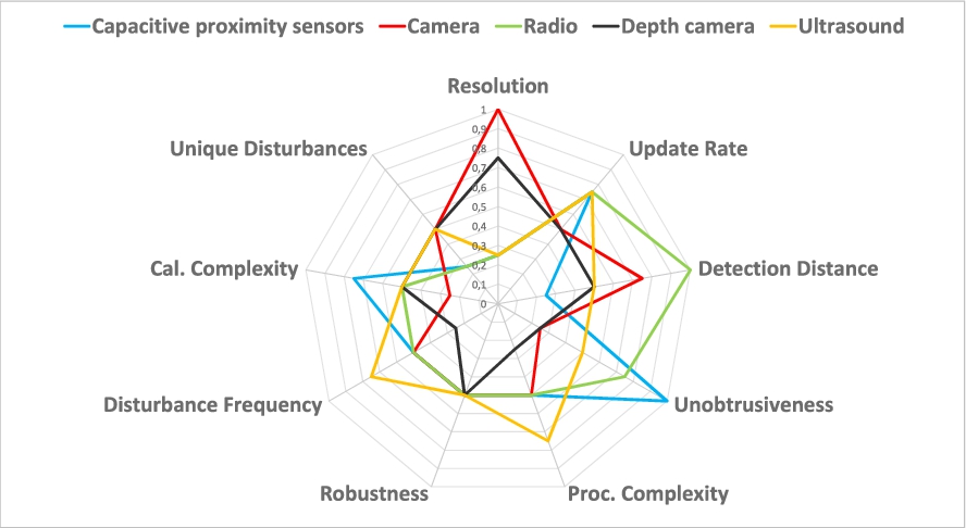
Radar chart, visualizing the results of Table 8.

As future work we want to improve our verification by using survey data to determine a more definite set of sensor features. For this task we may set up an online questionnaire and send it to other researchers in the domain of smart environments. Additionally, we would like to start cooperating with researchers from different fields, to evaluate if the benchmarking model can be easily transferred to more domains, for example robotics or human-computer interaction.

References

Ballagas,

Borchers,

Rohs and

J.G.

Sheridan, The smart phone: A ubiquitous input device, IEEE Pervasive Comput. 5(1) (2006), 70–77. doi:10.1109/MPRV.2006.18.

Bao and

S.S.

Intille, Activity recognition from user-annotated acceleration data, in: Proceedings PERVASIVE, 2004, pp. 1–17.

Barrett and

Omote, Projected capacitive touch screens, Inf. Disp. 1975 (2010).

Barsocchi,

Chessa,

Furfari and

Potorti, Evaluating ambient assisted living solutions: The localization competition, IEEE Pervasive Comput. 12(4) (Oct. 2013), 72–79. doi:10.1109/MPRV.2013.23.

Bertozzi and

Broggi, GOLD: A parallel real-time stereo vision system for generic obstacle and Lane detection, IEEE Trans. Image Process. 7(1) (1998), 62–81. doi:10.1109/83.650851.

Braun, Application and validation of capacitive proximity sensing systems in smart environments, Doctoral dissertation, TU Darmstadt, Darmstadt, 2014.

Braun,

Heggen and

Wichert, CapFloor – A flexible capacitive indoor localization system, in: Proceedings Evaluating AAL Systems Through Competitive Benchmarking. Indoor Localization and Tracking, 2012, pp. 26–35. doi:10.1007/978-3-642-33533-4_3.

Braun,

Wichert,

Kuijper and

D.W.

Fellner, A benchmarking model for sensors in smart environments, in: Proceedings AmI International, 2014, pp. 242–257.

Braun,

Wichert,

Kuijper and

D.W.

Fellner, Capacitive proximity sensing in smart environments, J. Ambient Intell. Smart Environ. (2015).

10.

Bulling,

J.A.

Ward,

Gellersen and

Troster, Eye movement analysis for activity recognition using electrooculography, IEEE Trans. Pattern Anal. Mach. Intell. 33(4) (2011), 741–753. doi:10.1109/TPAMI.2010.86.

11.

R.C.

Camp, Benchmarking: The Search for Industry Best Practices That Lead to Superior Performance, Quality Press, Milwaukee, 1989.

12.

Cheng,

Amft and

Lukowicz, Active capacitive sensing: Exploring a new wearable sensing modality for activity recognition, in: IEEE Pervasive Computing, Springer, 2010, pp. 319–336. doi:10.1007/978-3-642-12654-3_19.

13.

Chintalapudi,

Padmanabha Iyer and

V.N.

Padmanabhan, Indoor localization without the pain, in: Proceedings MobiCom, 2010, pp. 173–184.

14.

D.J.

Cook and

S.K.

Das, How smart are our environments? An updated look at the state of the art, Pervasive Mob. Comput. 3(2) (2007), 53–73. doi:10.1016/j.pmcj.2006.12.001.

15.

Coradeschi and

Saffiotti, Symbiotic robotic systems: Humans, robots, and smart environments, IEEE Intell. Syst. 21(3) (2006), 82–84. doi:10.1109/MIS.2006.59.

16.

Cowie,

Douglas-Cowie,

Tsapatsoulis,

Votsis,

Kollias,

Fellenz and

J.G.

Taylor, Emotion recognition in human-computer interaction, IEEE Signal Process. Mag. 18(1) (2001), 32–80. doi:10.1109/79.911197.

17.

L.E.

Crawford,

Huttenlocher and

P.H.

Engebretson, Category effects on estimates of stimuli: Perception or reconstruction? Psychol. Sci. 11(4) (2000), 280–284. doi:10.1111/1467-9280.00256.

18.

Crolotte, Issues in benchmark metric selection, in: TPC Technology Conference, 2009, pp. 146–152.

19.

J.J.

Dongarra,

Luszczek and

Petitet, The LINPACK benchmark: Past, present and future, Concurr. Comput. Pract. Exp. 15(9) (2003), 803–820. doi:10.1002/cpe.728.

20.

J.L.

Fleiss, Measuring nominal scale agreement among many raters, Psychol. Bull. 76(5) (1971), 378. doi:10.1037/h0031619.

21.

H.-W.

Gellersen,

Beigl and

Krull, The MediaCup: Awareness technology embedded in an everyday object, in: Proceedings Handheld and Ubiquitous Computing, 1999, pp. 308–310. doi:10.1007/3-540-48157-5_30.

22.

D.F.

Glas,

Kanda,

Ishiguro and

Hagita, Simultaneous people tracking and localization for social robots using external laser range finders, in: Proceedings IEEE/RSJ International Conference on Intelligent Robots and Systems, 2009, pp. 846–853.

23.

Grosse-Puppendahl,

Berghoefer,

Braun,

Wimmer and

Kuijper, OpenCapSense: A rapid prototyping toolkit for pervasive interaction using capacitive sensing, in: Proc. PerCom, 2013, pp. 152–159.

24.

Grosse-Puppendahl,

Berlin and

Borazio, Enhancing accelerometer-based activity recognition with capacitive proximity sensing, in: Proceedings AmI International, 2012, pp. 17–32.

25.

Grosse-Puppendahl,

Braun,

Kamieth and

Kuijper, Swiss-cheese extended: An object recognition method for ubiquitous interfaces based on capacitive proximity sensing, in: Proc. CHI, 2013, pp. 1401–1410.

26.

J.L.

Henning, SPEC CPU2000: Measuring CPU performance in the new millennium, Computer (Long. Beach. Calif.) 33(7) (2000), 28–35.

27.

M.E.

Hoque,

Courgeon,

J.-C.

Martin,

Mutlu and

R.W.

Picard, Mach: My automated conversation coach, in: Proceedings UbiComp, 2013, pp. 697–706.

28.

Jafari,

Mtenzi,

O’Driscoll,

Fitzpatrick and

O’Shea, Measuring privacy in ubiquitous computing applications, Int. J. Digit. Soc. 2(3) (2011), 547–550.

29.

Jain, The Art of Computer Systems Performance Analysis, Vol. 182, John Wiley & Sons, Chichester, 1991.

30.

Khosrowabadi,

H.C.

Quek,

Wahab and

K.K.

Ang, EEG-based emotion recognition using self-organizing map for boundary detection, in: Proceedings ICPR, 2010, pp. 4242–4245.

31.

Landsiedel,

Wehrle and

Götz, Accurate prediction of power consumption in sensor networks, in: Proc. Workshop on Embedded Networked Sensors, 2005.

32.

Lauterbach and

Steinhage, SensFloor^® – A large-area sensor system based on printed textiles printed electronics, in: Proceedings AAL-Kongress, 2009.

33.

B.C.

Lewis and

A.E.

Crews, The evolution of benchmarking as a computer performance evaluation technique, MIS Q. (1985), 7–16. doi:10.2307/249270.

34.

MacLachlan, Spread spectrum capacitive proximity sensor, Human Condition Wiki, 2004, [Online]. Available: http://humancond.org/wiki/user/ram/electro/capsense/0main.

35.

Majewski,

Braun,

Marinc and

Kuijper, Visual support system for selecting reactive elements in intelligent environments, in: Proceedings International Conference on Cyberworlds, 2012, pp. 251–255.

36.

Mitra and

Acharya, Gesture recognition: A survey, IEEE Trans. Syst. Man, Cybern. Part C Appl. Rev. 37(3) (2007), 311–324. doi:10.1109/TSMCC.2007.893280.

37.

Nakashima,

Aghajan and

J.C.

Augusto, Handbook of Ambient Intelligence and Smart Environments, Springer, 2009.

38.

Olsson,

Kärkkäinen,

Lagerstam and

Ventä-Olkkonen, User evaluation of mobile augmented reality scenarios, J. Ambient Intell. Smart Environ. 4(1) (2012), 29–47.

39.

Oreifej and

Liu, Hon4d: Histogram of oriented 4d normals for activity recognition from depth sequences, in: Proceedings CVPR, 2013, pp. 716–723.

40.

Pirkl and

Lukowicz, Resonant magnetic coupling indoor localization system, in: Proceedings Evaluating AAL Systems Through Competitive Benchmarking, 2013, pp. 59–62.

41.

Poslad, Ubiquitous Computing: Smart Devices, Environments and Interactions, Wiley.com, 2011.

42.

Pu,

Gupta,

Gollakota and

Patel, Whole-home gesture recognition using wireless signals, in: Proceedings MobiCom, 2013, pp. 27–38.

43.

Ranganathan,

Al-Muhtadi,

Biehl,

Ziebart,

R.H.

Campbell and

Bailey, Towards a pervasive computing benchmark, in: Proceedings PerCom, 2005, pp. 194–198.

44.

R.M.

Santos,

K.M.

de Oliveira,

R.M.C.

Andrade,

I.S.

Santos and

E.R.

Lima, A quality model for human-computer interaction evaluation in ubiquitous systems, in: Latin American Conference on Human Computer Interaction, 2013, pp. 63–70.

45.

A.N.

Shirehjini and

Nazari, A novel interaction metaphor for personal environment control: Direct manipulation of physical environment based on 3D visualization, Comput. Graph. 28(5) (Oct. 2004), 667–675. doi:10.1016/j.cag.2004.06.006.

46.

J.E.

Smith, Characterizing computer performance with a single number, Commun. ACM 31(10) (1988), 1202–1206. doi:10.1145/63039.63043.

47.

J.R.

Smith, Electric field imaging, Doctoral dissertation, Massachusetts Institute of Technology, 1999.

48.

P.-H.

Tsai,

T.-Y.

Chen,

C.-R.

Yu,

C.-S.

Shih and

J.W.S.

Liu, Smart medication dispenser: Design, architecture and implementation, IEEE Syst. J. 5(1) (2011), 99–110. doi:10.1109/JSYST.2010.2070970.

49.

Valtonen,

Maentausta and

Vanhala, TileTrack: Capacitive human tracking using floor tiles, in: Proceedings PerCom, 2009, pp. 1–10.

50.

R.P.

Weicker, Dhrystone: A synthetic systems programming benchmark, Commun. ACM 27(10) (1984), 1013–1030. doi:10.1145/358274.358283.

51.

Weiser, The computer for the 21st century, Sci. Am. 265(3) (1991), 94–104. doi:10.1038/scientificamerican0991-94.

52.

White, Windows Experience Index: An In-Depth Look, 2006, [Online]. Available: http://blogs.windows.com/windows/archive/b/windowsvista/archive/2006/09/22/windows-experience-index-an-in-depth-look.aspx.

53.

J.S.

Wilson, Sensor Technology Handbook, Elsevier, 2004.

54.

Wilson and

Shafer, XWand: UI for intelligent spaces, in: Proceedings CHI, Vol. 5, 2003, pp. 545–552.

55.

Wimmer and

Boring, HandSense: Discriminating different ways of grasping and holding a tangible user interface, in: Proceedings TEI, 2009, pp. 359–362.

56.

Ye,

Dobson and

McKeever, Situation identification techniques in pervasive computing: A review, Pervasive Mob. Comput. 8(1) (2012), 36–66. doi:10.1016/j.pmcj.2011.01.004.

57.

K.P.

Yeo,

Nanayakkara and

Ransiri, StickEar: Making everyday objects respond to sound, in: Proceedings UIST, 2013, pp. 221–226.

58.

T.G.

Zimmerman,

Lanier,

Blanchard,

Bryson and

Harvill, A hand gesture interface device, ACM SIGCHI Bulletin 17(4) (1986), 189–192. doi:10.1145/30851.275628.

		Camera			Ultrasound

		$a = 1$	$a = 5$	$a = 10$	$a = 1$	$a = 5$	$a = 10$
Hand Gesture	$m_{b}$	1.03	1.16	1.34	1.05	1.28	1.63
Hand Gesture	$m_{b, norm}$	1.00	1.00	1.00	1.00	1.00	1.00
Identification	$m_{b}$	0.99	0.95	0.90	1.07	1.40	1.97
Identification	$m_{b, norm}$	0.96	0.82	0.66	1.01	1.05	1.10
Obstacle Avoidance	$m_{b}$	0.97	0.86	0.74	1.09	1.54	2.37
Obstacle Avoidance	$m_{b, norm}$	0.94	0.73	0.54	1.03	1.16	1.34

Benchmarking sensors in smart environments – Method and use cases

Abstract

Keywords

1. Introduction

2. Related works

3.1. Indoor localization

3.2. Gestural interaction

3.3. Physiological sensing

3.4. Activity recognition

3.5. Smart appliances

3.6. Mobile devices

3.7. Autonomous systems

4. Sensor features

4.1. Selecting feature categories

4.2. Sensor performance characteristics

4.3. Pervasive metrics

4.4. Environmental characteristics

4.5. Discussion of feature selection

5. Benchmarking model

5.2. Modeling

5.3. Feature score normalization

5.4. Benchmark scoring

Table 3 The importance weighting of different applications, based on the features res upd det unob proc robu disfr calco uniql Hand Gesture ++ ++ - + o o + + - Identification -- - ++ ++ o ++ + - + Obstacle Avoidance - + - o + + ++ ++ +

1 http://dl.acm.org.

6.3. Discussion of search results

6.4. Querying scientific databases

6.6. Multiple benchmarks and confidence

7. Determining use cases for capacitive proximity sensors

Table 8 Feature weights for capacitive proximity sensors Capacitive proximity sensors res upd det unob proc robu disfr calco uniqd - + - ++ o o o + - Camera ++ o + - o o o - o Radio - + ++ + o o o o - Depth camera + o o - - o - o o Ultrasound - + o o + o + o o

9. Conclusion and future work

References

Table 3
The importance weighting of different applications, based on the features

res upd det unob proc robu disfr calco uniql

Hand Gesture ++ ++ - + o o + + -

Identification -- - ++ ++ o ++ + - +

Obstacle Avoidance - + - o + + ++ ++ +

¹
http://dl.acm.org.

Table 8
Feature weights for capacitive proximity sensors

Capacitive proximity sensors res upd det unob proc robu disfr calco uniqd

- + - ++ o o o + -

Camera ++ o + - o o o - o

Radio - + ++ + o o o o -

Depth camera + o o - - o - o o

Ultrasound - + o o + o + o o