An unsupervised technique to discretize numerical values by fuzzy partitions

Abstract

The numerical value discretization is a process that is performed in the data preprocessing phase of intelligent data analysis. Preprocessing phase is very relevant because the quality of the models obtained in data mining step depends on this phase. Value discretization is an important task in data preprocessing because not all data mining techniques can handle continuous values. In this paper an unsupervised technique to discretize continuous data values using fuzzy partitions is proposed. Specifically a clustering technique that gets fuzzy partitions is presented. In addition, to evaluate the behavior of the proposed technique a series of experiments have been proposed using a Extreme Learning Machine classifier and a committee of Extreme Learning Machine. Beside comparing with the K-means discretization technique. These experiments have been validated statistically obtaining the best results the approach proposed.

Keywords

Discretization fuzzy clustering membership function extreme learning machine data mining

1. Introduction

The discretization is a relevant task of data preprocessing within Intelligent Data Analysis. This task has as objective to transform the attributes with continuous values into discrete values, either through intervals or through fuzzy partitions. This discretization process is essential because there are data mining techniques that can not manage continuous values, these techniques can only handle categorical/discretized values some of these are: association rules, induction rules, Bayesian networks, some techniques of decision trees, random forest, etc. There are even data mining techniques, that being able to work with continuous values, obtain more satisfactory models working with discrete values. Between the advantages of dicretization it can be highlighted the capability to reduce the number of store data, to improve the interpretability both initial data and results obtained and the effectiveness and efficiency that will be established later in the application of data mining techniques. The effectiveness and efficiency caused by discretization favors to a certain extent the reduction of the computational cost [4,8].

In literature several taxonomies to classify the different discretization techniques can be found [22,35]. Without being exhaustive some of these classifications are analyzed taking into account the characteristics of them:

Static versus Dynamic: A static discretizer performs the learning task independent from the learning algorithm. A dynamic technique performs the discretization during the learning phase of the data mining technique.

Global or Local: Global discretization is performed when all the information is used to discretize. Local discretization technique only uses part of the information to perform the discretization process.

Supervised or Unsupervised: Unsupervised techniques do not consider the label class to perform the discretization. Supervised techniques need to evaluate the label class to perform the partition.

Univariate or Multivariate: Multivariate techniques create the initial cut point with all attributes simultaneously. The univariate techniques only consider an attribute each time.

Direct or Incremental: Direct techniques divide the range into k intervals simultaneously, requiring a criterion to determine the k value. By contrast, incremental discretizers begin with a simple discretization, and perform improvement process until a stop criterion is fulfill.

Splitting or Merging: Splitting discretizers create new intervals dividing the domain of the continuous values. Merging techniques create a number of intervals which are removing and merging to obtain the final partitions. Some techniques can be considered hybrid because they can alternate splits with merges in running time [8].

Evaluation measure: Discretizers can also classify considering the measure used to assess the partitions. Thus, some measure used are: information measure such as entropy and Gini Index, rough set measure, statistical measures, error in classification or binning that is the absence of measure.

Fuzzy or crisp: This type of discretization depends on the logic used (classical or fuzzy logic). The difference between a fuzzy discretization or a crisp discretization is the result of the intervals. When the discretization is fuzzy, the intervals overlap and a value may belong to more than one interval. On the contrary in a crisp discretization, the intervals are disjoint and a value can only belong to an interval.

Parametric or Nonparametric: A parametric discretizers need that users fix a maximum number of intervals. However, a nonparametric discretizer determines automatically the number of intervals to discretize a continuous attribute.

Top-Down or Bottom Up: This characteristic is usual in incremental discretizers, [8]. Top-down techniques start with an empty discretization and add new cut point during the discretization process. On the contrary, bottom up techniques start with all possible intervals, and during the discretization process, they are removing cut point, that means, merging intervals.

Stopping criteria: This characteristic is referred to the stop conditions of the discretization process, some of this conditions are confidence thresholds [17], inconsistency ratios [5] or the Minimum Description Length measure [6].

Disjoint or Non-disjoint: Disjoint techniques divide the domain in crisp partitions, that means, in intervals. Non-disjoin techniques allow the overlapping between partitions. Usually, fuzzy discretization techniques are non-disjoin.

Nominal or Ordinal: Nominal discretizers divide the domain in nominal qualitative values. On the contrary, ordinal discretizers transform the domain in ordinal qualitative values. This last type of discretization is not very common.

The assessment of the partitions can be performed using different method such as number of intervals, inconsistency, predictive classification rate or time requirements. The most commonly used method is usually the classification predictive classification rate, therefore, we use them for our experiments. In this paper, a modification of the Fuzzy C-Means (FCM) technique [34] is used to develop a fuzzy and unsupervised discretization algorithm. This proposal is based on Cauchy distribution to discretize numerical values. To assess the approach datasets from UCI repository, [20] are used. The results obtained after comparing with the classical discretization technique based on K-means (KM) algorithm [12] are satisfactory. The paper is organized as follow. In Section 2 a brief review of some work on discretization is carried out. Then, in Section 3 the discretization technique proposed is explained. Next, Section 4, the classifier used to assess the quality of discretization is exposed. Finally, in Section 5 and 6 the experiments, conclusion and future works are presented, respectively.

2. Background

Different discretization techniques can be found in literature due to the fact that there are not an universal technique to obtain categorical values that works properly with any data mining method. Thus, in [25], several discretization techniques are evaluated to use the most suitable for clinic data. The discretization performed by these authors is crisp and the techniques used are both supervised and unsupervised. In their conclusions, the authors affirm that supervised discretization is more particular and unsupervised is more general and it can be applied in more domains.

In [21], a fuzzy and unsupervised discretization is presented. In this work the discretization process is performed by means of clustering technique, selecting initial clustering centers by large density area and using density function as samples’ weights to reduce effectively noise interference. Then, the compatibility of decision table in rough set theory is used as criteria to adjust dynamically the parameters of the algorithm to achieve optimal discretization effect. Another clustering technique is exposed in [1]. In this case, the authors develop a clustering technique as a discretization technique to recognize solar images, extracting texture features of these images. In [23] a non-parametric discretization technique for continuous values with missing data is presented. This technique uses the statistical technique z-score with an index measure to impute the missing data values for numeric or continuous attributes. In [39] an iterative and novel scheme to dicretize is presented. This method dynamically discretizes the continuous random variables in intervals at each iteration. The interactive method is focused on estimating the likelihood of low-probability failure events instance of focusing on getting the overall shape of the distribution correct. The method is assessed using a dynamic Bayesian Networks.

The authors of [15] present a supervised and multivariate discretization algorithm called SMDNS based on rough sets, which is derived from the traditional algorithm naive scaler. This method simultaneously considers all attributes, that is, takes into account the interdependence among various attributes. The method iteratively merges adjacent intervals of continuous values according to a given criterion. A hybrid discretization method for naïve Bayesian classifiers is presented in [36]. The propose discretizer uses a nonparametric measure to assess the dependence level between a continuous attribute and the class.

In [37] other algorithm to perform fuzzy partition is developed. Specifically authors expose a two-step method to create membership function. In the first step the method divides domain of continuous attributes in intervals and then in the second step the different membership functions are created. For creating the membership functions they use four different measures, particularly partition width, standard deviation of examples, coverage rate of neighbor partitions and Entropy Based Fuzzy Partitioning. Another discretization technique that uses different measures to perform the discretization process is presented in [16]. In this case, the authors propose a weighted hybrid discretization technique based on entropy and contingency coefficient.

In [3], a method to discretize continuous attribute is proposed. This method performs the discretization during the learning phase of a decision tree. Specifically to perform the discretization the authors propose an extension of the method Ant Colony Decision Tree. In [19] a self-adaptive discretization method is proposed to discretize continuous values for association rule. The self-adaptive method proposed creates partitions which can give a high confidence to the calculated association rule while guaranteeing the relatively high support.

3. Discretization technique

This section describes the proposed discretization technique based on clustering analysis. This technique can be categorized according to the above categorization as a global, unsupervised and fuzzy discretization technique.

Clustering analysis consists of dividing a data into several clusters where data in same cluster have high similarity while data in different clusters are distinct each other. KM algorithm is one of the most popular clustering methods, [12]. This algorithm starts by guessing k cluster centers and then iterates the following steps until convergence is achieved. Each cluster is built by assigning each instance to the closest cluster center and each cluster center is replaced by the mean of the elements belonging to that cluster. Traditional clustering methods, such as KM, each instance is assigned to one cluster in an unequivocal way. As opposed to this, in fuzzy clustering an instance x may belong to different clusters at the same time, and the degree to which it belongs to the kth cluster is expressed in terms of a membership degree. Consequently, the boundary of single clusters and the transition between different clusters are usually soft rather than abrupt. An example of fuzzy clustering would be FCM. The k-means algorithm has been extended to the fuzzy c-means algorithm by Bezdek in the early eighties [2] and is one of the most widely used fuzzy clustering methods. The cluster analysis FCM aims to find the patterns in data by processing a range of clusters by the calculation of distances of registers to clusters centers through the FCM algorithm.

Consider the dataset X to a set of n instances $X = {x_{1}, x_{2}, \dots, x_{n}} \subset R^{F}$ and P to be a set of k clusters such that $P = {c_{0}, c_{1}, \dots, c_{k - 1}}$ . Each instance $x_{j}$ is composed of a set of numerical features $x_{i j}$ . A value $x_{i j}$ is the ith feature, with $i = 1, \dots, p$ , associated with the instance j. Each of the data points such as $x_{i}$ may belong to one or more clusters depends on its degree of membership. Point $x_{i}$ belongs to cluster $c_{j}$ as long as its degree of membership to $c_{j}$ is more than zero.

Clustering a dataset requires finding the center of each cluster and deciding to which cluster each point belongs to. In FCM to find the center of a cluster, the sum of the distance between points in the cluster and its center is used as criterion. The criteria is represented by an objective function, J, which needs to be minimized with respect to P, a fuzzy c-partition of the dataset, and V, a set of c prototypes for cluster centers $V = {v_{1}, v_{2}, \dots, v_{c}} \subset R^{F}$ . In general, fuzzy clustering techniques minimize an objective function that determines the centroid or prototypes of each cluster. In [7], FCM algorithm uses the objective function given by: $\begin{matrix} (1) & J_{m} (P, v) = \sum_{x \in X} \sum_{k = 1}^{c} u_{x k}^{m} \cdot d_{x k}^{2} \end{matrix}$

The formula incorporates the fuzzy membership function $u_{x k}$ of the instance x to the group k: $\begin{matrix} (2) & u_{x k} = \frac{1}{1 + d_{x k}^{2}} \end{matrix}$ $d_{x k}$ is the Mahalanobis distance [24] from the instance x to the cluster which prototype is $v_{k}$ and an additional parameter m, as a weighted exponent for the fuzzy membership. Parameter m is the value that determines the degree to which partial members of cluster affect the clustering results. At the beginning of the process V is initialized with some prototype values that get updated during the process.

The function J is minimized by using the following equations for updating the membership degrees and V iteratively until $| v_{i} - v_{i - 1} | < ϵ$ .

The μFCM algorithm is derived from FCM algorithm, and μFCM is explained in [34]. This algorithm is the approach proposed in this paper to be applied as discretization technique instead of classifier technique. Between others differences, the membership function of μFCM ( $u_{x k}$ ) is deduced from the study of the objective function in [7], and these grades of membership are calculated as follow: $\begin{matrix} (3) & u_{x k} = \frac{μ_{x k}^{3 / 2} \sqrt{g_{k}^{- 1}}}{\sum_{j = 1}^{c} μ_{x j}^{3 / 2} \sqrt{g_{j}^{- 1}}} \end{matrix}$ which express the relative deviation of each group k, where the parameters $g_{k}$ and $g_{j}$ are the determinants of the fuzzy covariance matrix [10] at k and j, respectively and the function μ is a type of Cauchy distribution, and it is calculated as: $\begin{matrix} (4) & μ_{x k} = \frac{1}{1 + d_{x k}^{2}} \sqrt{g_{k}} \end{matrix}$

The fuzzy covariance matrix at cluster k is defined, in [10], as: $\begin{matrix} (5) & G_{k} = [\frac{\sum_{x \in X} u_{x k}^{2} (x^{α} - v_{k}^{α}) (x^{β} - v_{k}^{β})}{\sum_{x \in X} u_{x k}^{2}}], \end{matrix}$ where $x = (x^{1}, \dots, x^{F})$ , $R^{F}$ and $v_{k} = (v_{k}^{1}, \dots, v_{k}^{F})$ , $R^{F}$ is the prototype of cluster k. And $g_{k} = det (G_{k})$

The membership of all samples to all clusters defines a partition matrix as $U = [u_{x k}]$ .

So that, the objective function (1) is rewritten here as: $\begin{matrix} (6) & J_{(k)} = \sum_{x \in X} \frac{1}{{(1 + d_{x k}^{2})}^{3 / 2}} \sqrt{g_{k}} d_{x k}^{2} \end{matrix}$

The μFCM algorithm computes interactively the clusters centers coordinates from a previous estimate of the partition matrix as: $\begin{matrix} (7) & v_{k} = \frac{\sum_{x \in X} u_{k x} \cdot x_{k}}{\sum_{x \in X} u_{k x}} \end{matrix}$

Algorithm 1 shows the μFCM process. It is an iterative process where one standard value is included in the computation, ϵ. The algorithm is composed of the following steps:

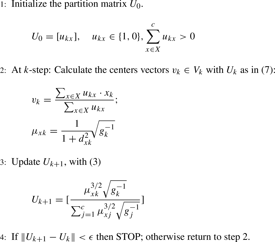
Algorithm 1

Algorithm μFCM

Fig. 1.

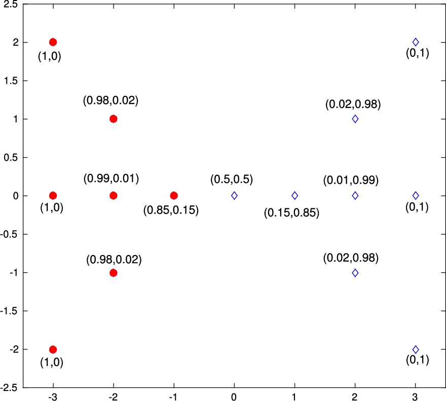
Illustration for the sample of Butterfly dataset. The point and diamond differentiate the two groups classified with K-means algorithm, while the pairs in brackets indicate the probabilities of diffuse belonging of each point to each of the two groups in which the set has been segmented.

The μFCM algorithm is used as a discretization technique by applying it to each attribute separately. In this way, the values are classified in three clusters (good-regular-bad). From this performance, a “weight” is assigned to every value of the attribute selected, which corresponds with the μ-values. This process avoids the possibility of correlation, to avoid problems with the classifier.

Let’s exemplify the difference between KM and μFCM. Figure 1 shows the two groups that the KM algorithm obtains. These groups are represented by points and diamonds. The algorithm places the point $(0, 0)$ indistinctly a few times in one group and sometimes in the other group, the equidistant with the rest of the points indicates indifference before assigning it to one or the other. For its part, the algorithm μFCM performs a diffuse classification, which allows assigning a probability of belonging to each of the two groups. This classification is depicted in Fig. 1 by probabilities of belonging shown in brackets. The algorithm μFCM obtains in the classification of the point $(0, 0)$ a probability of 0.5 of belonging to the group of the left and of 0.5 to the one of the right. Both algorithms (KM and μFCM) classify with absolute probabilities, 1 or 0, the points located on the abscissa $- 3$ and 3. However, the points located on the abscissa $- 2$ and 2 differ in the case of the classification by μFCM, because of the proximity to the centers detected by μFCM, $v_{1}$ $(- 2.21, 0)$ and $v_{2}$ $(2.21, 0)$ .

Table 1

μ-function and KM Classification for the sample of Butterfly dataset

x	μ-function		KM

	$μ_{x v_{1}}$	$μ_{x v_{2}}$	Cluster1	Cluster2
$(- 3, 2)$	0.0983	0.0035	1	0
$(- 3, 0)$	0.3893	0.0038	1	0
$(- 3, - 2)$	0.0983	0.0035	1	0
$(- 2, 1)$	0.4373	0.0068	1	0
$(- 2, 0)$	0.9551	0.0071	1	0
$(- 2, - 1)$	0.4373	0.0068	1	0
$(- 1, 0)$	0.1806	0.0154	1	0
$(0, 0)$	0.0428	0.0428	0	1
$(1, 0)$	0.0154	0.1806	0	1
$(2, - 1)$	0.0068	0.4373	0	1
$(2, 0)$	0.0071	0.9551	0	1
$(2, 1)$	0.0068	0.4373	0	1
$(3, - 2)$	0.0035	0.0983	0	1
$(3, 0)$	0.0038	0.3893	0	1
$(3, 2)$	0.0035	0.0983	0	1

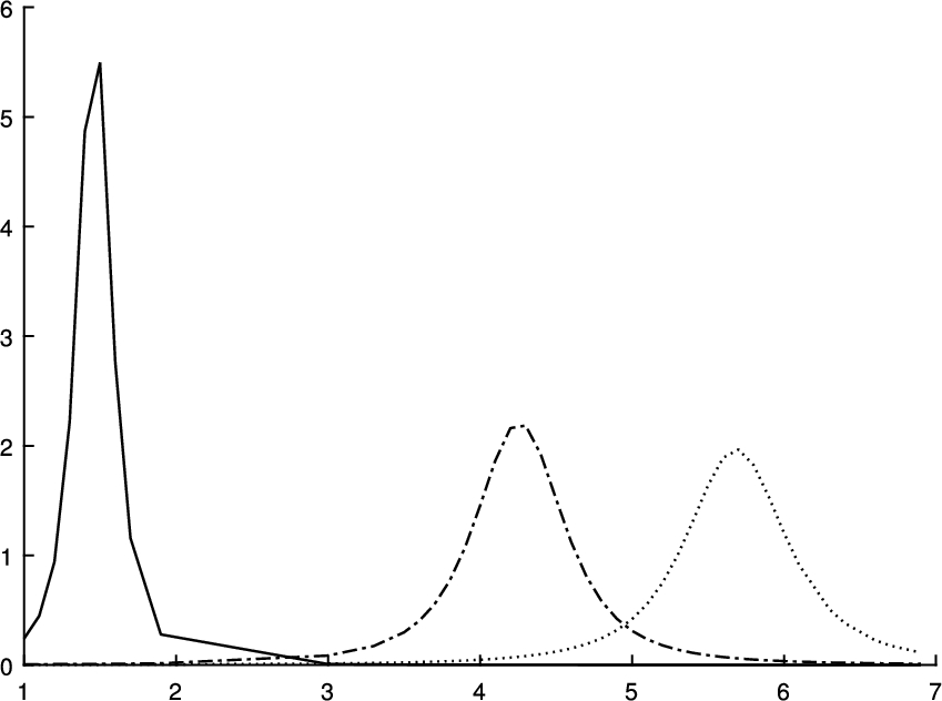
Table 1 shows the values obtain for μ-function for each of the centers $v_{1}$ $(- 2.21, 0)$ and $v_{2}$ $(2.21, 0)$ of the Butterfly sample, after applying the algorithm μFCM. These values are in opposition to those obtained by the KM that are shown in the same table. These values represent the discretization perform for each algorithm.

In order to illustrate the process, the example of Iris Data has been considered. The attributes sepal length, sepal width, petal length and petal width are discretized independently, and the interpolation of μ-functions are represented in Figs 2, 4, 5 and 6 respectively.

Fig. 2.

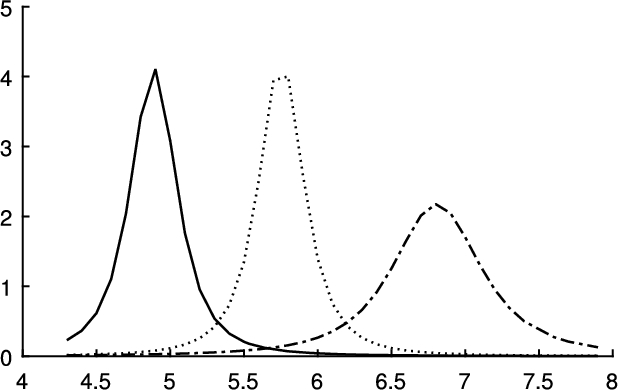
A linear interpolation of the μ-function for the sepal length attribute in cm.

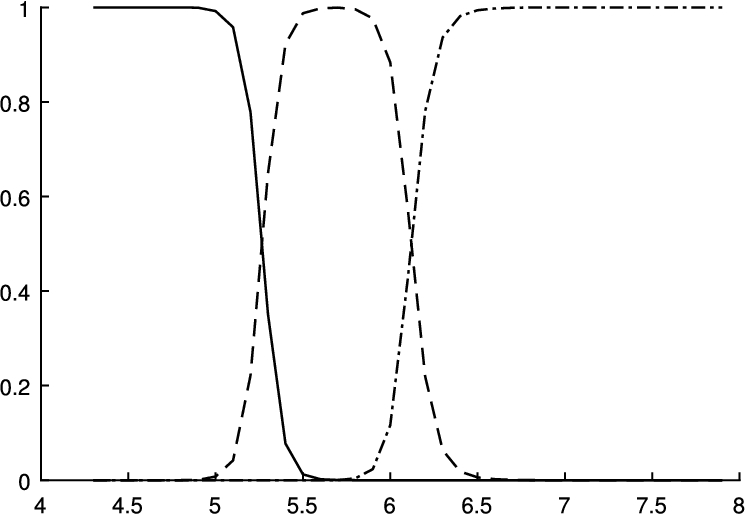
The μ-function for each cluster created by the μFCM algorithm for the sepal length attribute is represented in Fig. 2. The graphic depicts three clusters represented by the prototypes in the maxims of the function. The μFCM algorithm uses the showed probabilities values of the μ-function in Fig. 2. In this way, for a 6.5 cm sepal length, the membership probability value is 98.17%, $u_{6.5, 3} = 0.9817$ , represented by the biggest prototype, with respect to the cluster represented by the central prototype is 1.69%, $u_{6.5, 2} = 0.0169$ ; and 0% with respect to the farthest cluster, $u_{6.5, 1} = 0$ .

Fig. 3.

The membership probability for the sepal length attribute.

Usually, fuzzy clustering algorithms return the membership probabilities using graphics as Fig. 3. The values obtained through the μ-function of the μFCM algorithm are used and represented in Fig. 2.

In the following Figs 4, 5, 6, the μ-functions for the rest of attributes are represented. Each cluster is represented by a different line types and each prototype is identified by the maximum of the function.

Using the same notation employed to explain Fig. 2, Fig. 4 shows for a 2.4 cm sepal width the μ-function values obtained are $μ_{2.4, 1} = 2.7616$ , $μ_{2.4, 2} = 0.0397$ and $μ_{2.4, 3} = 0.0385$ .

Fig. 4.

A linear interpolation of the μ-function for the sepal width attribute in cm.

Fig. 5.

A linear interpolation of the μ-function for the petal length attribute in cm.

In Fig. 4, it is shown for example that for a 4 cm petal length the following μ-function values are obtained: $μ_{4, 1} = 0.0017$ , $μ_{4, 2} = 1.4510$ and $μ_{4, 3} = 0.0475$ .

Fig. 6.

A linear interpolation of the μ function for the petal width attribute cm.

Finally, Fig. 6 shows for example that for a 1.6 cm petal width the following μ-function values are obtained: $μ_{1.6, 1} = 0.0037$ , $μ_{1.6, 2} = 0.884$ and $μ_{1.6, 3} = 0.3480$ .

Once the proposed μFCM discretization technique is detailed, the following section presents the classifier used to evaluate the quality and suitability of this technique. In addition, this evaluator is also used in the comparison with the KM technique. The classifier used as evaluator is the Extreme Learning Machine.

4. Classifier

For Multilayer Perceptron (MLP), Extreme Learning Machine (ELM) provides a fast and efficient training [14]. Formalized by Huang [9,13], it is demonstrated that the ELM is an universal approximation for a wide range of random computational nodes. The MLP input weights are fixed to random values, so, the output weights can be easily obtained using the pseudo-inverse of the hidden neurons outputs matrix H for a given training set. Given a set of N input vectors, an MLP can approximate N cases with zero error, $\sum_{i = 1}^{N} ‖ y_{i} - t_{i} ‖ = 0$ , being $y_{i}$ the output network for the input vector $x_{i}$ with target vector $t_{i}$ . Thus, there exist $β_{j}$ , $w_{j}$ and $b_{j}$ such that, $\begin{matrix} (8) & \begin{array}{l} y_{i} = \sum_{j = 1}^{M} β_{j} f (w_{j} \cdot x_{i} + b_{j}) = t_{i}, \\ i = 1, \dots, N . \end{array} \end{matrix}$ where $β_{j} = {[β_{j 1}, β_{j 2}, ..., β_{j m}]}^{T}$ is the weight vector connecting the jth hidden node with the output nodes, $w_{j} = {[w_{j 1}, w_{j 2}, ..., w_{j n}]}^{T}$ is the weight vector connecting the jth hidden node and the input nodes, and $b_{j}$ is the bias of the jth hidden node.

The previous N equations can be expressed by: $\begin{matrix} (9) & H B = T, \end{matrix}$ where $\begin{array}{l} (10) & \begin{array}{l} H (w_{1}, \dots, w_{M}, b_{1}, \dots, b_{M}, x_{1}, \dots, x_{N}) \\ = {[\begin{matrix} f (w_{1} \cdot x_{1} + b_{1}) & \dots & f (w_{M} \cdot x_{1} + b_{M}) \\ ⋮ & \dots & ⋮ \\ f (w_{1} \cdot x_{N} + b_{1}) & \dots & f (w_{M} \cdot x_{N} + b_{M}) \end{matrix}]}_{N \times M} \end{array} \\ (11) & B = {[\begin{matrix} β_{1}^{T} \\ ⋮ \\ β_{M}^{T} \end{matrix}]}_{M \times m} and T = {[\begin{matrix} t_{1}^{T} \\ ⋮ \\ t_{N}^{T} \end{matrix}]}_{N \times m} \end{array}$ where $H \in R^{N \times M}$ is the hidden layer output matrix of the MLP, $B \in R^{M \times m}$ is the output weight matrix, and $T \in R^{N \times m}$ is the target matrix of the N training cases. The MLP training is given by the solution of the least square problem of (9). The optimal output weight layer is $\hat{B} = H^{†} T$ , where $H^{†}$ is the Moore-Penrose pseudo-inverse [32]. ELM for training MLPs can be therefore summarized as shown in Algorithm 2.

Algorithm 2

Extreme Learning Machine (ELM)

A problem that presents the ELM is to obtain the number of neurons for the MLP. This requires a pruning method for the ELM. Although there are several pruning methods [26–31], the most commonly used, to avoid the exhaustive search for the optimal value of M, is the ELM Optimally Pruned (OP-ELM) [29]. The OP-ELM sorts the hidden neurons (previously has been initialized to a very high initial number) according to their importance to solve the problem [33]. The pruning of neurons is done by choosing that combination of neurons that provides lower Leave-One-Out error [29]. For more detail, OP-ELM is summarized in Algorithm 3.

Algorithm 3

Optimally Pruned-ELM (OP-ELM)

Each input characteristic provides a membership function. The union of all of them is trained with the OP-ELM (Fig. 7). This paper also discusses the use of a combination of MLPs (trained width OP-ELM). The use of multiple models may often improve the performance with respect to an individual model [11,38]. Such combination of networks are called committees. A combination of MLPs is presented where each network has been trained with a single input characteristic, because μFCM works individually with each input feature by generating a membership function for each of the partitions created. This allows to create a network committee formed by many networks as the input features have the database, and where each feature has been transformed into its membership function, thus forming the network input. Once trained each network, this provides us with an output that will be the input for a new network, newly trained with OP-ELM, that provides the classification accuracy (Fig. 8). It should be noted that once each network has been trained, the importance of that input for the new network is verified. In this way, networks that do not generate good performance are discarded, which may be due to the fact that this input characteristic is not relevant to learning the model. This transformation of each input characteristic to its membership function provided by the μFCM could be used to make a selection of relevant input characteristics because it is done individually for each input.

Fig. 7.

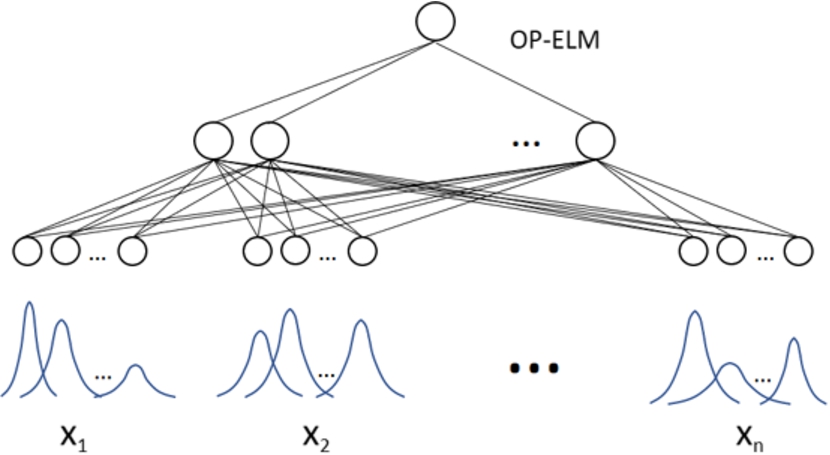
Single classifier model. Each input is transformed with the membership function, thus forming the input of the network to be trained with the OP-ELM algorithm.

Fig. 8.

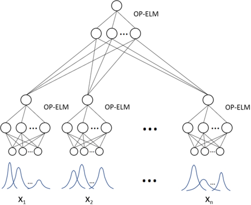
Network committee used to train the model. Each input characteristic is trained by one network and its output is the input of the final network. All are trained with the OP-ELM algorithm.

5. Experimental results

The proposed discretization technique is evaluated using the ELM explained in Section 4. Table 2 shows the number of input features and number of classes for each dataset, these datasets are obtained from UCI repository [20].

Table 2
Dataset Description

Name Nu N.Classes

Iris 4 3

Wine 13 3

Vertebral Column 6 2

Banknote Authentication 4 2

Thyroid Disease 5 3

Occupancy Detection 4 2

Name	Nu	N.Classes
Iris	4	3
Wine	13	3
Vertebral Column	6	2
Banknote Authentication	4	2
Thyroid Disease	5	3
Occupancy Detection	4	2

The proposed technique (μFCM) is compared with the classic technique K-means (KM). On the one hand, the goodness of the techniques is assessed by a Leave-One-Out Cross-Validation repeated 30 times. On the other hand, a series of tests have been carried out in order to validate the best number of partitions to divide each one of the numerical attributes of the datasets. In this way, in this study it is taken into account not only the accuracy obtained in classification but also the interpretability of the results obtained.

Fig. 9.

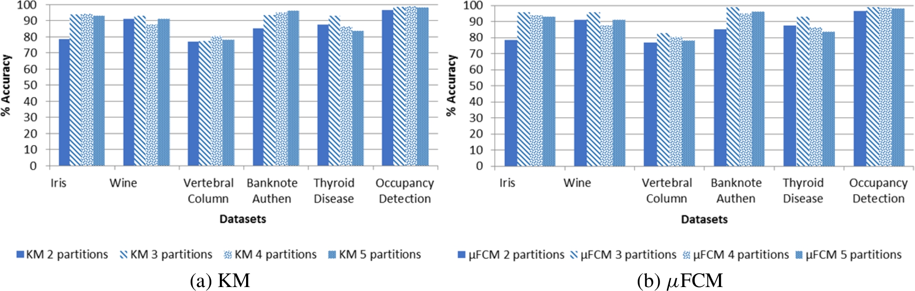
Comparative for the KM and μFCM technique with different granularity in partitions.

Figure 9 shows the results obtained by KM (Fig. 9(a)) and μFCM (Fig. 9(b)) techniques using different granularity in partitions. Specifically, a division of 2, 3, 4 and 5 partitions have been used for each attribute. In general, this figure shows how the division into 3 partitions achieves the best results.

Table 3

Experimental results with three partitions

Dataset	KM	μFCM
Iris	$93.64 \pm 0.72$	$95.62 \pm 0.38$
Wine	$92.79 \pm 1.17$	$95.51 \pm 0.40$
Vertebral Column	$77.08 \pm 0.41$	$82.60 \pm 0.92$
Banknote Authen.	$84.98 \pm 0.09$	$98.89 \pm 0.15$
Thyroid Disease	$92.81 \pm 0.67$	$93.01 \pm 0.58$
Occupancy Detection	$96.43 \pm 0.21$	$98.09 \pm 0.09$

Fig. 10.

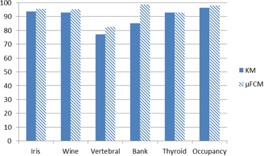
Graphical comparison of the validation of the techniques KM and μFCM.

The best results obtained with three partitions are shown in Table 3, where it can be seen the classification accuracy with its associated standard deviation. It can be clearly seen that μFCM gets better results. More graphically, the results are shown in Fig. 10.

To validate this assertion, a non parametric statistical test has been performed. Specifically, the Wilcoxons Signed Ranks Test is used [18]. This test compares two paired groups and can be used to test where the null hypothesis indicate that two populations have the same continuous distribution.

Table 4 shows the p-value and the negative and positive rank and the statistical Z that is based on negative rank. As it is shown in this table, the technique μFCM is compared statistically with KM technique, obtaining a p-value of 0.028, that means the null hypothesis (the result means of both technique are similar) is rejected with 97% of confidence level. According to the statistical Z, the technique with more satisfactory results is μFCM. In addition to the quantitative results, it must be also highlighted the qualitative part of them. Considering that these results are achieved with three partitions for numerical attributes, it can be indicated that the results obtained are satisfactory and interpretable, since for each attribute all the continuous values are reduced to 3 values.

Table 4

Statistical test result

μFCM-KM	Results
Negative ranks	0.0
Positives ranks	6.0
Ties	0.0
$Z^{a}$	−2.201
p-value	0.028

In addition to the results obtained, a committee system to validate the results has been used. The use of a committee system has been tested with Iris and Vertebral datasets. Figures 11 and 12 show the classification of each individual network for each input features. It can be seen that features number 3 and 4 are the most relevant for Iris data, Fig. 13 shows the accuracy classification (in %) for iris data, where it has trained with the KM, μFCM and two different committees: where only the input feature number 2 has been removed, and another where the features 1 and 2 have been removed. It can be observed as improving the learning by eliminating the less relevant input features. Nevertheless, all features are similar for accuracy classification in the vertebral dataset (see Fig. 12), so, Fig. 14 shows the KM, μFCM and several different committees: with all features and removing each feature separately. It can be observed that improves learning by eliminating the fourth input characteristic.

Fig. 11.

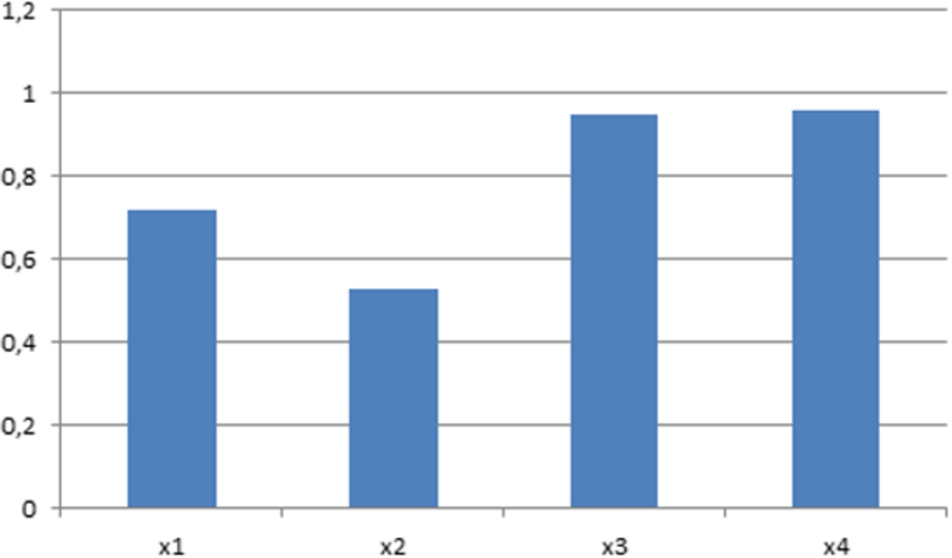
Iris data. Detail of the learning of each input characteristic for the network committee. It can be seen that the best classification accuracy is for x3 and x4.

Fig. 12.

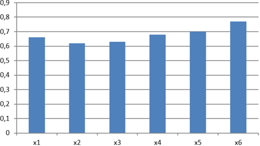
Vertebral Column dataset. Detail of the learning (accuracy in %) of each input characteristic for the network committee.

Fig. 13.

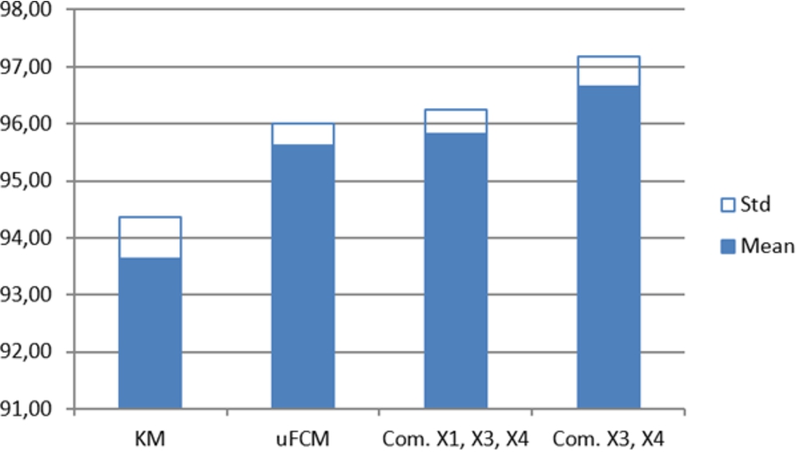
Iris data. Classification accuracy (mean and standard deviation) with KM algorithms, μFCM and μFCM committee with all inputs features and removing each feature.

Fig. 14.

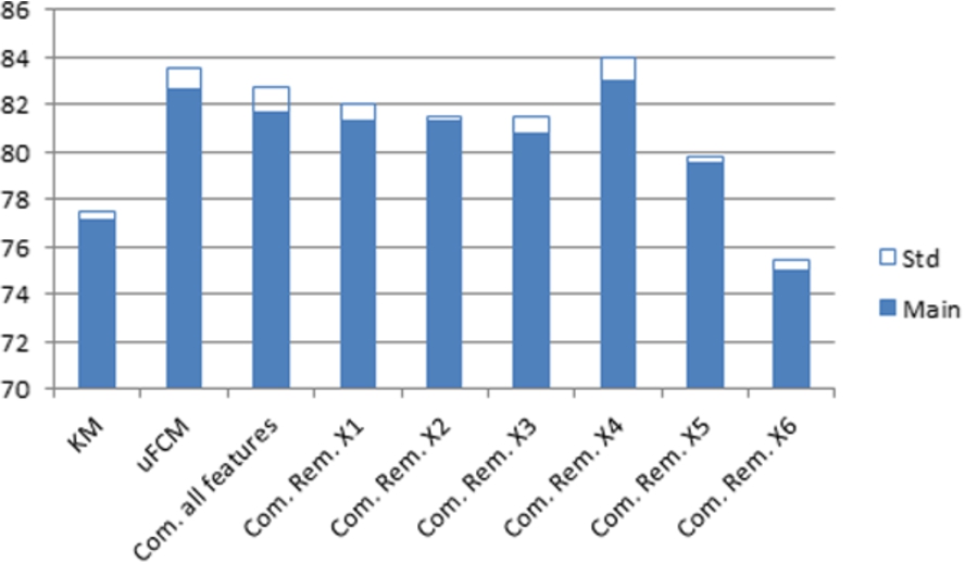
Vertebral Column dataset. Classification accuracy (mean and standard deviation) with KM algorithms, μFCM and μFCM committee.

6. Conclusions and future work

In this paper, a discretization technique based on fuzzy clustering is proposed. This technique is based on the μFCM algorithm to perform a numerical discretization using Cauchy distribution. In order to assess the discretization technique a ELM classifier and a committee of ELM classifiers are applied. The classifiers are also applied to asses the discretization obtained for the KM technique. In addition, from a qualitative point of view, the best granularity has also been evaluated to carry out discretization. For this purpose, different granularities have been evaluated regarding the number of partitions for each numerical attribute. This evaluation has made it possible to verify that in general terms satisfactory results are obtained with 3 partitions in each attribute. This gives us a great interpretability of the results, since the technique allows to transform continuous values for each attribute into discrete values through 3 partitions. Therefore, from a qualitative point of view, the results are quite interesting. Besides, the results of the comparison between μFCM and KM techniques have been statistically validated, where the proposed technique (μFCM) obtaining the best results with 97% of confidence level.

As future work, the new objective functions of the discretization clustering technique will be implemented. Also, the option to discretize using probabilistic functions for the clustering technique instead of the membership function used in this study can be explored and analyzed.

Footnotes

Acknowledgement

This work is supported by the Spanish MINECO under grant TIN2016-78799-P (AEI/FEDER, UE).

References

J.M.

Banda and

R.A.

Angryk, On the effectiveness of fuzzy clustering as a data discretization technique for large-scale classification of solar images, in: Fuzzy Systems, 2009. FUZZ-IEEE 2009. IEEE International Conference on, IEEE, 2009, pp. 2019–2024. doi:10.1109/FUZZY.2009.5277273.

J.C.

Bezdek,

Ehrlich and

Full, FCM: The fuzzy c-means clustering algorithm, Computers & Geosciences10(2–3) (1984), 191–203. doi:10.1016/0098-3004(84)90020-7.

Boryczka and

Kozak, An adaptive discretization in the ACDT algorithm for continuous attributes, in: Computational Collective Intelligence. Technologies and Applications, 2011, pp. 475–484.

Butterworth,

D.A.

Simovici,

G.S.

Santos and

Ohno-Machado, A greedy algorithm for supervised discretization, Journal of biomedical informatics37(4) (2004), 285–292. doi:10.1016/j.jbi.2004.07.006.

M.R.

Chmielewski and

J.W.

Grzymala-Busse, Global discretization of continuous attributes as preprocessing for machine learning, International journal of approximate reasoning15(4) (1996), 319–331. doi:10.1016/S0888-613X(96)00074-6.

Fayyad and

Irani, Multi-interval discretization of continuous-valued attributes for classification learning, in: International Joint Conf. Artificial Intelligence (IJCAI), 1993, pp. 1022–1029.

Flores-Sintas,

J.M.

Cadenas and

Martin, Partition validity and defuzzification, Fuzzy Sets and Systems112(3) (2000), 433–447. doi:10.1016/S0165-0114(98)00004-9.

Garcia,

Luengo,

J.A.

Sáez,

Lopez and

Herrera, A survey of discretization techniques: Taxonomy and empirical analysis in supervised learning, IEEE Transactions on Knowledge and Data Engineering25(4) (2013), 734–750. doi:10.1109/TKDE.2012.35.

G.B.

Guang-Bin and

Chen, Convex incremental extreme learning machine, Neurocomputing70(16) (2007), 3056–3062.

10.

D.E.

Gustafson and

W.C.

Kessel, Fuzzy clustering with a fuzzy covariance matrix, in: 1978 IEEE Conference on Decision and Control Including the 17th Symposium on Adaptive Processes, 1978, pp. 761–766. doi:10.1109/CDC.1978.268028.

11.

L.K.

Hansen and

Salamon, Neural network ensembles, IEEE transactions on pattern analysis and machine intelligence12(10) (1990), 993–1001. doi:10.1109/34.58871.

12.

J.A.

Hartigan, Clustering Algorithms, 99th edn, John Wiley & Sons, Inc., New York, NY, USA, 1975. ISBN 047135645X.

13.

G.B.

Huang,

Wang and

Lan, Extreme learning machines: A survey, International Journal of Machine Learning and Cybernetics2(2) (2011), 107–122. doi:10.1007/s13042-011-0019-y.

14.

G.B.

Huang,

Q.Y.

Zhu and

C.K.

Siew, Extreme learning machine: Theory and applications, Neurocomputing70(1) (2006), 489–501. doi:10.1016/j.neucom.2005.12.126.

15.

Jiang and

Sui, A novel approach for discretization of continuous attributes in rough set theory, Knowledge-Based Systems73 (2015), 324–334. doi:10.1016/j.knosys.2014.10.014.

16.

Y.-G.

Jung,

K.M.

Kim and

Y.M.

Kwon, Using weighted hybrid discretization method to analyze climate changes, in: Computer Applications for Graphics, Grid Computing, and Industrial Environment, Springer, 2012, pp. 189–195. doi:10.1007/978-3-642-35600-1_28.

17.

Kerber, Chimerge: Discretization of numeric attributes, in: Proceedings of the Tenth National Conference on Artificial Intelligence, Aaai Press, 1992, pp. 123–128.

18.

W.H.

Kruskal, Historical notes on the Wilcoxon unpaired two-sample test, Journal of the American Statistical Association52(279) (1957), 356–360. doi:10.1080/01621459.1957.10501395.

19.

Li,

Zhang,

Zhou and

Zheng, A new approach of self-adaptive discretization to enhance the apriori quantitative association rule mining, in: Intelligent System Design and Engineering Application (ISDEA), 2012 Second International Conference on, IEEE, 2012, pp. 44–47. doi:10.1109/ISdea.2012.540.

20.

Lichman, UCI machine learning repository (http://archive.ics.uci.edu/ml). University of California, Irvine, School of Information and Computer Sciences, Irvine, CA, 2013.

21.

Liu,

Li and

Zhang, A soft partition discretization algorithm based on fuzzy clustering, in: 2012 9th International Conference on Fuzzy Systems and Knowledge Discovery, 2012, pp. 419–423. doi:10.1109/FSKD.2012.6234116.

22.

Liu,

Hussain,

C.L.

Tan and

Dash, Discretization: An enabling technique, Data mining and knowledge discovery6(4) (2002), 393–423. doi:10.1023/A:1016304305535.

23.

Madhu

et al., A non-parametric discretization based imputation algorithm for continuous attributes with missing data values, International Journal of Information Processing8(1) (2014), 64–72.

24.

P.C.

Mahalanobis, On the generalised distance in statistics, in: Proceedings National Institute of Science, India, Vol. 2, 1936, pp. 49–55, http://ir.isical.ac.in/dspace/handle/1/1268 .

25.

D.M.

Maslove,

Podchiyska and

H.J.

Lowe, Discretization of continuous features in clinical datasets, Journal of the American Medical Informatics Association20(3) (2013), 544–553. doi:10.1136/amiajnl-2012-000929.

26.

Mateo and

Lendasse, A variable selection approach based on the delta test for extreme learning machine models, in: Proceedings of the European Symposium on Time Series Prediction, 2008, pp. 57–66.

27.

Miche,

Bas,

Jutten,

Simula and

Lendasse, A methodology for building regression models using extreme learning machine: OP-ELM., in: ESANN, 2008, pp. 247–252.

28.

Miche and

Lendasse, A faster model selection criterion for OP-ELM and OP-KNN: Hannan–Quinn criterion., in: ESANN, Vol. 9, 2009, pp. 177–182.

29.

Miche,

Sorjamaa,

Bas,

Simula,

Jutten and

Lendasse, OP-ELM: Optimally pruned extreme learning machine, IEEE Transactions on Neural Networks21(1) (2010), 158–162. doi:10.1109/TNN.2009.2036259.

30.

Miche,

Sorjamaa and

Lendasse, OP-ELM: Theory, experiments and a toolbox, in: International Conference on Artificial Neural Networks, Springer, 2008, pp. 145–154.

31.

H.J.

Rong,

Y.S.

Ong,

A.H.

Tan and

Zhu, A fast pruned-extreme learning machine for classification problem, Neurocomputing72(1) (2008), 359–366. doi:10.1016/j.neucom.2008.01.005.

32.

Serre, Matrices: Theory and Applications, Springer, New York, 2002.

33.

Similä and

Tikka, Multiresponse sparse regression with application to multidimensional scaling, in: International Conference on Artificial Neural Networks, Springer, 2005, pp. 97–102.

34.

Soto,

Flores-Sintas and

Palarea-Albaladejo, Improving probabilities in a fuzzy clustering partition, Fuzzy Sets and Systems159(4) (2008), 406–421. doi:10.1016/j.fss.2007.08.016.

35.

Wang,

P.S.

Yu and

Han, Data mining and knowledge discovery handbook, in: Data Min. Knowl. Discov. Handb, 2010, pp. 1269–1277.

36.

T.-T.

Wong, A hybrid discretization method for naïve Bayesian classifiers, Pattern Recognition45(6) (2012), 2321–2325. doi:10.1016/j.patcog.2011.12.014.

37.

Zeinalkhani and

Eftekhari, Fuzzy partitioning of continuous attributes through discretization methods to construct fuzzy decision tree classifiers, Information Sciences278 (2014), 715–735. doi:10.1016/j.ins.2014.03.087.

38.

Z.-H.

Zhou,

Wu and

Tang, Ensembling neural networks: Many could be better than all, Artificial intelligence137(1–2) (2002), 239–263.

39.

Zhu and

Collette, A dynamic discretization method for reliability inference in dynamic Bayesian networks, Reliability Engineering & System Safety138 (2015), 242–252. doi:10.1016/j.ress.2015.01.017.

An unsupervised technique to discretize numerical values by fuzzy partitions

Abstract

Keywords

1. Introduction

2. Background

3. Discretization technique

Table 2 Dataset Description Name Nu N.Classes Iris 4 3 Wine 13 3 Vertebral Column 6 2 Banknote Authentication 4 2 Thyroid Disease 5 3 Occupancy Detection 4 2

Footnotes

Acknowledgement

References

Table 2
Dataset Description

Name Nu N.Classes

Iris 4 3

Wine 13 3

Vertebral Column 6 2

Banknote Authentication 4 2

Thyroid Disease 5 3

Occupancy Detection 4 2