The semantics of extensive quantities within geographic information

Abstract

The next generation of Geographic Information Systems (GIS) is anticipated to automate some of the reasoning required for spatial analysis. An important step in the development of such systems is to gain a better understanding and corresponding modeling practice of when to apply arithmetic operations to quantities. The concept of extensivity plays an essential role in determining when quantities can be aggregated by summing them, and when this is not possible. This is of particular importance to geographic information systems, which serve to quantify phenomena across space and time. However, currently, multiple contrasting definitions of extensivity exist, and none of these suffice for handling the different practical cases occurring in geographic information. As a result, analysts predominantly rely on intuition and ad hoc reasoning to determine whether two quantities are additive. In this paper, we present a novel approach to formalizing the concept of extensivity. Though our notion as such is not restricted to quantifications occurring within geographic information, it is particularly useful for this purpose. Following the idea of spatio-temporal controls by Sinton, we define extensivity as a property of measurements of quantities with respect to a controlling quantity, such that a sum of the latter implies a sum of the former. In our algebraic definition of amounts and other quantities, we do away with some of the constraints that limit the usability of older approaches. By treating extensivity as a relation between amounts and other types of quantities, our definition offers the flexibility to relate a quantity to many domains of interest. We show how this new notion of extensivity can be used to classify the kinds of amounts in various examples of geographic information.

Keywords

Extensive quantities definition geocomputation semantic labeling of geodata

1. Introduction

An important distinction in geographic analysis is between those quantities that can and those that cannot be summed during spatial aggregation. These are known as, respectively, extensive and intensive quantities. Human analysts can intuitively tell how a quantity should be processed when two regions are merged. Two temperature values of two spatial regions, for example, should not be summed, although they may be treated as a weighted sum when the regions are aggregated. In geographic information systems (GIS), however, the values may be represented by the same concrete data types, and thus cannot be systematically distinguished. Current GIS lack a method for automating aggregations because we lack a theory of extensivity that can tell us under which circumstances we can sum up quantities in space, time, and other kinds of domains.

One fruitful way to capture extensivity is in terms of a relation between different domains of measurement (Scheider and Huisjes, 2019). This notion of extensivity entails that quantities can be aggregated if they share domains of measurement by which they can be controlled and measured in a coordinated manner. Controlling quantities need to be separated from each other, and both controlling and controlled quantities need to be additive in a way that preserves sums. For example, the population of Europe can be aggregated with the population of Africa, as both populations are part of the world population, but not with the summed GDP of Africa, which does not share the same measurement domain. Here, the spatial administrative units are controlling and population counts are measured. However, Europe’s population should also not be aggregated with the population of Utrecht, because even though they share the same measurement domains, Utrecht is already a part of Europe. While such observations may seem intuitive, the sciences still lack a formalization of these kinds of considerations. Most existing definitions of extensivity that reached prominence are either too restrictive or too vague, leaving room for inadequate interpretation (See Section 2.1). Moreover, existing definitions of extensivity seem to misconceptualize its relational character. For over a century, the prevalent idea was that extensivity is a fixed property of scales originating from the existence of a sum operator or the way they were derived from fundamental measurement units. However, as our examples about population and temperature illustrate, though the underlying measurement scales come with sum operations in all cases, it is not always meaningful to sum up quantities when merging regions. Furthermore, in this article, we make the case for the view that all quantities can be extensive with respect to some and intensive with respect to other quantities. For example, temperature, which is regularly used as an example of an intensive quantity, turns out to be extensive with respect to thermal energy. A measurement value of temperature can be obtained by dividing a value of thermal energy by the product of mass and heat capacity. Imagine the temperature of a heating system is measured before and after an amount of energy is added, and assume that all other quantities are held constant.1

¹
For convenience, also assume the heating system perfectly retains all energy (i.e. there is no loss of energy over time).

When the mass and heat capacity are held constant, increases in thermal energy translate into homomorphic increases in temperature.

A concise yet flexible definition of extensivity would enable determining whether spatial arithmetic is applicable or not based on classifying quantities accordingly. In previous work, we (Scheider and Huisjes, 2019) have illustrated the merit of spatial extensivity in the context of geographic information and mapping and managed to automatically distinguish extensive from intensive quantities with high accuracy. However, though this work forms a basis for the current article, it was never formalized and does not account for quantities that are additive in domains other than space, such as e.g. time. Also, if we recognize there are multiple dimensions of extensivity, new ways to categorize quantities emerge. A water flow accumulation is extensive in space and time, the cost of a stay at a hotel is extensive in time and some monetary currency, and the cost of rental cars is extensive in time (i.e. the duration of renting), space (i.e. the amount of kilometers driven) and the amount of cars (i.e. renting two cars is more expensive than one). Extensivity offers a new semantic dimension by which data can be discovered and processed. A definition of extensivity would therefore also contribute to a data-driven science (Hey et al., 2009; Gahegan, 2020) by determining which arithmetic operations can be applied to available quantities.

In this article, we suggest a first-order formalization of quantity domains as a basis for a higher-order, relational definition of extensivity using quantities as controls and measures. We then demonstrate how this definition allows us to define various subclasses of extensive measurement across geographic information examples in terms of an OWL2

Web Ontology Language, see e.g. Hitzler et al. (2009).

pattern with subsumption reasoning. Though our theory as such is not restricted to geographic quantities, the concepts of control and measure on which it is based are central for geographic information, as explained below. Our contribution is therefore threefold and provides answers to the following questions:

In which way can extensivity be formalized in terms of measurement, control and summation of quantities? Which classes of quantity domains need to be distinguished for this purpose?

How can extensive quantities be measured across time, space and content, within the context of geographic information?

How can extensive geographic measurements be systematically categorized according to different kinds of controls and measures, and how can this be used to automatically classify map examples?

Our answers contribute important formal distinctions to measurement ontology which are currently lacking. While measurement theory formalizes levels of measurement scales in terms of the operations they preserve on particular quantity domains (Suppes and Zinnes, 1962), ontologies like DOLCE (Masolo et al., 2003), or, more recently, the FOUnt ontologies (Aameri et al., 2020), relate the underlying quantity domains to each other and ontological “background” phenomena like endurants, perdurants, and their properties. However, so far, we do not know of any attempt at formalizing the notion of extensivity as a relational concept, and in the context of geographic information. Furthermore, while the current ontological accounts provide useful insights and models about concepts of measurement, they also come with certain restrictions that make it difficult to account for the notion of extensivity.

First of all, most existing measurement ontologies lack the formal depth to specify the distinctions needed for capturing the notion of extensivity. For example, lightweight ontologies such as the OM-ontology (Rijgersberg et al., 2013) lack a rigorous formalization of the underlying concepts and are instead primarily focused on terminological conventions (Balazs, 2008) in specific application areas (Steinberg et al., 2016). Furthermore, foundational ontologies that would provide the formal depth come with certain problematic assumptions and ontological commitments. For one, even though there are notions that resemble our notion of amount in both DOLCE and the FOUnt ontologies, they are largely centered around the idea of ‘physical matter’ or ‘stuff’ constituting endurants. Examples would be the amount of clay constituting a statue or the amount of wine in a bottle, which are modeled as phenomena that can be considered snapshots in time. However, for geographic information, we need to consider the possibility of forming amounts across time as well as space. For example, quantifications of water running through a waterfall (Galton and Mizoguchi, 2009) or of traffic flowing into a city presuppose amounts in time as well as space. Second, even if including both endurants and perdurants as bearers of amounts, the notion of extensivity requires also a degree of arbitrariness of forming amounts, which stands in apparent contrast to the simple unity criteria for wholes within the boundaries of objects and events that are underlying DOLCE (Guarino et al., 2000). Consider the amount of population living close to a border or between two cities, the amount of water flowing through the waterfall in between two events, or the amount of space covered by an arbitrary circle around some point. These are relevant geographic examples that illustrate that the unity criteria for amounts go beyond the constitution of particular objects or events within the limits of their boundaries. Of course, we can always create objects with unity for arbitrary portions of amounts (cf. Guizzardi (2010)), however, this appears redundant in light of a theory of extensive amounts.

The extensivity concept suggested in this article accounts for some of this flexibility in terms of a generalized notion of amounts that is used to control other measurable quantities, following earlier ideas of Sinton (1978). With this approach, arbitrary divisions of amount portions can control arbitrary quantities, not only by way of objects. This closely corresponds to the way how quantification is done in a GIS (cf. Chrisman (2002)). To this end, we formalize two classes of quantity domains (amounts and magnitudes) which are used to define extensivity on a higher level and then introduce a simple design pattern that can be used to classify various examples of extensive measurement across time and space within geographic information.

The rest of the paper is organized as follows. First, we review what is known about extensivity, quantities and measurement. Second, we reinterpret Sinton (1978)’s three roles of measurement (i.e. measure, control, constant) and show in an informal manner how they can be used to specify extensivity relations. Third, we present a formalized algebraic theory of extensivity as a relation between a measure and one or more controls, including automatic proofs of theorems. Fourth, we translate this basic theory into a lightweight OWL pattern adding classes specific for geographic information. We then propose twelve categories of measurement of extensive quantities in the context of geographic information and show how extensivity classes can be automatically inferred. Finally, we shortly discuss the implications of our findings and conclude by answering the posed research questions.

2. Extensivity, quantities, and measurement

We start with reviewing existing literature on extensivity and quantities and scrutinize the underlying approaches for our purpose. Furthermore, we critically examine Sinton’s notion of controlled measurement, and discuss how it can be exploited for our purpose.

2.1. Extensivity and intensivity

The concept of extensivity originates from the fields of Physics and Chemistry where it is used to describe the mathematical nature of properties. Its introduction and axiomatization can be accredited to scholars in the first half of the twentieth century (Hölder, 1901; Tolman, 1917; Campbell, 1920). Tolman (1917) envisions extensivity as a way to describe phenomena whose measures are naturally additive. Of all phenomena he identifies only five as extensive in this sense, namely length, time interval, mass, electric charge, and entropy. For a contemporary definition of extensivity, scholars often refer to the green book of the International Union of Pure and Applied Chemistry (IUPAC), which describes an extensive quantity as “a quantity that is additive for independent, non-interacting subsystems” (Cohen et al., 2007). In practice, there seems to be an informal consensus that only properties like volume or mass are considered extensive. Even within this consensus, disagreement exists about what physical properties extensivity depends on. A number of papers from Physics and Chemistry try to address the confusion surrounding the concept (Redlich, 1970; Canagaratna, 1992; Mannaerts, 2014). Mannaerts (2014) finds that the expressions ‘extensive quantity’ and ‘extensive property’ are used interchangeably — He favours the use of the term ‘extensive quantity’ — and that some use additivity to define extensivity (i.e. the sizes of two quantities can be added up during aggregation) while others use proportionality (i.e. a quantity inextricably changes relative to changes of another quantity). Some scholars limit extensivity to a relation of properties with respect to mass, while others relate them to the amount of substance or volume (Mannaerts, 2014). Restricting extensivity to a specific kind of physical substance deviates considerably from the original theory (Tolman, 1917), which holds that properties may be extensive also with respect to time or entropy. Not only do scholars consider different properties as the source of extensivity, they also disagree on the mechanisms of extensivity itself.

The concept of an extensive quantity is opposed to that of an intensive quantity, which has been defined as “a quantity that is independent of the extent of the system” (Cohen et al., 2007). Tolman (1917) argues that, except for his five fundamental quantities, all quantities are intensive, because they are in some way derived from the five fundamental quantities. A speed, for example, is found by dividing a length (i.e. the distance) by a time interval. Some scholars hold that not all quantities are either extensive or intensive. They argue that some quantities are expressed as conjugates (Alberty, 1997) or composites, which have characteristics of both.

2.2. Quantities

Quantities are described as “...that by which a thing is said to be large or small, or to have part outside of part, or to be divisible into parts” (Kocourek, 2018). Specifications of quantities are frequently present in spoken language (Talmy, 1978). For example, the sentence ‘The flock of birds flew over the wide river’ not only specifies two different entities (i.e. ‘birds’ and ‘river’), but also details their quantities (i.e. ‘flock’ and ‘wide’) and their interrelation (i.e. ‘over’).

From a semantic viewpoint, quantities should be distinguished from numbers, which are mathematical objects for representing measurement results, and measurement units, which indicate the measurement system a quantity is measured in .3

³
Different measurement systems (or reference systems) (Chrisman, 2002) can represent the same kind of quantity. For example, the meter scale and the feet scale both represent the same quantity of lengths.

In measurement theory, it is common to classify measurement systems using measurement levels, which range from nominal through ordinal and interval to ratio (Stevens et al., 1946). These levels encode increasing amounts of information of a quantity, by preserving operations for class membership, order, relative position and absolute effect of a quantity (Suppes and Zinnes, 1962). Chrisman (1998) proposed to extend these levels with counts, degrees of class membership, cyclical ratio, derived ratio, and immutable absolute measures, like probability.

Quantities can be negative and can be on a linear scale of measurement. For example, walking backwards for twenty meters can be seen as a negative quantity of forward movement associated with the number −20 and the unit ‘meters’. The term magnitude, also called impact or size, is used to measure a quantity on a linear scale. Scholars sometimes distinguish multitudes from magnitudes (Lachmair et al., 2018). Shortly put, multitudes refer to collections of discrete entities (e.g. a collection of cars), while magnitudes capture linearly order-able phenomena (e.g. the length of a road). Plewe (2019) in addition refers to continuously divisible quantities as ‘geographic masses’ and illustrates the relevance of this concept for Geography. Our approach (see below) can be used to make these notions more precise, by formalizing what extensive quantities are in general, and how they are controlled in geographic information.

Information about the extensivity of a quantity is closely related to its part-whole relations. Such relations are commonly considered homeomerous with respect to its parts, meaning that all parts are of the same kind of quantity as the whole (Gerstl and Pribbenow, 1993). For instance, sectioning a portion of water results in sub-portions of water. According to Guizzardi (2010), homeomerous part-whole relations can be modelled as maximally self-contained mereological sums (i.e. aggregations of the subquantities) or by means of containment (e.g. a bottle of water). This approach implies that parts of a quantity, also referred to as pieces (Lowe, 1998), are only instantiated if there is a need. For example, a body of water may be subdivided into its parts to identify sweet water and salt water if necessary, but this is not required for capturing the water concept. Guizzardi’s mereological approach also works for universal properties and classes. For example, a car is a member of the collection of all cars (i.e. the class of ‘cars’), and the mass of said car is a part of the set of all mass in the universe (i.e. the ‘mass’ property). The DOLCE ontology makes use of this principle of extensionality (Masolo et al., 2003; Gangemi et al., 2001). Recently, work in the context of the FOUnt ontologies (Aameri et al., 2020) has shown that formally adequate models of physical quantities need to incorporate formal relations between property bearers, mereologies in different quantity dimensions (Ru and Gruninger, 2017), and quantities represented by measurement scales. Going beyond existing ontologies of units of measure (Rijgersberg et al., 2013), the definition of formal properties of quantities thus requires further concepts.

For extensivity, mereological relations are essential because they specify whether two quantities are distinct, whether and how much they overlap and whether one quantity contains another. For example, a university may host multiple lectures at once, meaning they share the same quantity of time. Summing the total time of the lectures may indicate how long it would hypothetically take to attend all lectures (e.g. 400 hours), but this does not correspond to the extent of time that is actually occupied by these lectures (e.g. 3 hours). If two lectures with a duration of 2 hours each overlap for 1 hour, they together occupy 3 hours in time. Claramunt and Jiang (2001) show that such relations are not limited to space or time, but also exist between conjunctions of both.

2.3. Measurement of quantities

Sinton (1978) is well-known for his idea that the measurement of spatial information requires attribute information about the space, time and theme components of the recording. Sinton argues that during any measurement each one of these three components fills the role of the constant, the control or the measure:

The constant component, also referred to as the support or the fixed component, does not change at any point in the measurement process.

The control component is allowed to vary over its measurement scale at the observer’s discretion.

The measure component is observed and its variation with respect to the control is recorded.

Take the example of a precipitation measurement. Precipitation is commonly measured with a rain gauge. This rain gauge fixes the spatial extent of the precipitation measure, e.g., to 1 dm². The amount of water falling into the rain gauge is then measured in mm and converted to kg or liters over a variable amount of time, e.g. an hour or a day (Chrisman, 2002). With an established constant (i.e. space) and control (i.e. time), it is possible to measure an amount of rainfall in mm. Sinton’s work contains two important messages: 1) a measurement of a phenomenon always requires other variables to be controlled, and 2) geographic information always contains a combination of spatial information, obtained through the measurement of locations and regions, temporal information, obtained through the measurement of the progress of time, and thematic information, obtained through measuring some content of spatial or temporal regions.

Chrisman (2002) argues that apart from space, time and theme, there is another kind of control, namely control by relationship. For example, the measurement of a flow of export products from countries to one another first requires establishing a relation between the countries (in the sense of a spatial network, cf. (Kuhn, 2012)). Although this is a relevant case of extensivity (Scheider and de Jong, 2022), we leave the study of network-controlled extensive quantities for future work.

The roles of measure, control and constant are essential for our purpose, because they aptly capture how quantities can play different roles in defining extensivity. Measured quantities are extensive if they are controlled in a particular way by other quantities. However, Sinton’s idea requires some scrutiny before it can be applied to quantities. For one, the fillers of roles are by no means restricted to the three components of geographic information. Many measurements ignore one or more of the components. For example, when measuring the duration of a given lecture, there is no need to take the size of the lecture room or the didactic ability of the lecturer into account. In fact, only the time interval at which the lecture happens is required as a control to measure duration. Note also that in this example, the time component appears as both measure and control at once. It is clear therefore that the components space, time and theme are much too coarse to distinguish the relevant quantities, and thus for capturing extensivity. We therefore adopt three alterations of Sinton’s idea. Firstly, we interpret Sinton’s components as classes of quantities which might play a role or not in a given measurement. We thus allow for arbitrary combinations of quantities filling the roles in a single measurement. Secondly, we assume that quantities exert no influence on measurement (i.e. are kept constant) unless specified otherwise. This prevents the need for explicitly filling the constant role. And third, we formally distinguish subclasses of quantity domains to account for extensive measurements that can be made on a single one of Sinton’s dimensions.

3. A formal theory of extensive quantities

In the following, when we talk about quantities, we deviate from certain terminological habits in measurement theory and ontology of measurement, simply because we believe our usage is closer to the common understanding of a term. First, when we speak about a quantity, we mean an individual value of measurement, such as the value represented by 15 kg. This is close to everyday usage, such as in “the quantity of flour used to make this bread”. Correspondingly, we use the term quantity domain to talk about all elements of a domain of measurement, such as the kilogram scale (Probst, 2008). Second, we do not assume quantities are necessarily on linear measurement scales. In the example above, the quantity of flour is not the same as its value in kilograms, though it can be measured on the kilogram scale. This requires us to distinguish different kinds of quantity domains. In the following, we introduce a formal theory in First Order Logic (FOL) about quantity domains, and measurement functions as mappings between these. FOL is sufficient to reason about a single quantity domain, but strictly speaking, we go beyond FOL when quantifying over different domains. Free variables in propositions are implicitly all-quantified over a quantity domain. Axiom sets of all (sub)theories are provably consistent, and all theorems were automatically proven based on resolution using Prover9.4

⁴
https://www.cs.unm.edu/~mccune/prover9/

The scripts are available online.5

⁵

Amount theory: http://geographicknowledge.de/vocab/quantity_amount.txt.

⁶

Magnitude theory: http://geographicknowledge.de/vocab/quantity_magnitude.txt.

To get an overview of the following definitions, Table 1 provides a preliminary summary and exemplification of the main formal concepts that we introduce below. Each of the concepts in the table is also explained in the text.

Table 1

Preliminary summary of the main concepts

Concept	Description	Examples
Quantity	An individual value of a measurement that can be used to form sums.	A spatial region or its size or its proportion with respect to another region’s size.
Amount	An extensional mereological quantity whose domain forms a lattice.	A spatial region (=amount of space).
Magnitude	A linearly, monotonically ordered quantity.	The size of a spatial region or its proportion with respect to another region’s size.
Archimedean magnitude	A magnitude whose domain forms a vector space (can be summed and subtracted, but not multiplied)	The size of a spatial region.
Proportional magnitude	A magnitude whose domain forms a mathematical field (allowing for products and ratios)	The proportion of a region’s size with respect to another region’s size.
Quantity domain	A set of quantities together with operations on them (forming an algebra)	The set of all regions and the set of all region sizes are domains of quantities of space.
Control	The role of a quantity domain as a domain of measurement, i.e., a domain of a measurement function.	When measuring the amount of population within a region, the amount of space of that region is a control.
Measure	The role of a quantity domain as a range of measurement, i.e., a co-domain of a measurement function.	When measuring the amount of space occupied by an amount of people, the amount of space is a measure.

3.1. Quantities, amounts and magnitudes

Certain kinds of quantities can be added up to or removed from each other, resulting in a new quantity of which original quantities are parts. For example, a quantity of people can be added up to another quantity of people to form a total sum of people, and the original quantities are parts of the whole. We call quantities that can be added up in this way amounts. In our theory, this means that amounts can be summed, be subtracted from and be part of each other. In the following, we will motivate and illustrate the axioms with examples of amounts of space (E.g., spatial regions), amounts of time (E.g., time intervals), as well as amounts of matter and amounts of objects.7

⁷
In the following, we use the terms amounts of space and (spatial) regions and the terms amounts of time and (time) intervals interchangeably.

3.1.1. Theory of amounts (extensional mereological quantities forming a Boolean lattice)

The parthood relations of amounts are captured by mereological axioms. We assume an amount domain8

⁸
Many authors speak of dimensions of measurement rather than domains. We use the term ‘domain’, because we want to prevent the assumption of linearly ordered elements.

is a set with algebraic operations that satisfy the following partially ordered algebra:

Axiom 1.

Partial order of parthood $\begin{aligned} x \subseteq x Reflexivity \\ (x \subseteq y \land x \supseteq y) ⟹ x = y Antisymmetry \\ (x \subseteq y \land y \subseteq z) ⟹ x \subseteq z Transitivity \end{aligned}$

For example, if two amounts of sand are part of each other, they are identical, and parts of parts of an amount of sand are also parts of the former amount of sand. Based on this, we define the following predicates:

Definition 1.

Strict order and overlap $\begin{aligned} x \subset y ⟺ (x \subseteq y \land \neg (y \subseteq x)) Strict order \\ O (x, y) ⟺ \exists z (0 \subset z \land z \subseteq x \land z \subseteq y) Overlap \\ y \supset x ⟺ x \subset y Strictly greater than \\ y \supseteq x ⟺ x \subseteq y Greater than or equal \end{aligned}$

Strictly ordered amounts are not identical, meaning one is a proper part of the other, and overlapping amounts have a common part that is not empty (Casati et al., 1999).

Axiom 2.

Sums and differences $\begin{aligned} x + y = y + x Commutativity \\ (x + y) + z = x + (y + z) Associativity \\ x + 0 = x Identity + \\ x ∖ x = 0 Inverse \\ y ∖ 0 = y Identity Minus \end{aligned}$

Axiom 2 introduces operations for adding and subtracting amounts. Note the identity (empty) element 0 which can be added without changing anything and which results from subtractions of amounts from themselves. To give some motivation for these axioms, it is apparently irrelevant in which order we sum up amounts of sand. Furthermore, if we add/subtract no sand to/from an amount of sand, the amount is left unchanged. Furthermore, if we remove the entire amount of sand, nothing is left over. This apparently applies also in the case of spatial regions as well as time intervals.

In addition, we introduce a product operation for amounts, which is interpreted in terms of an intersection of two amounts. Intersection distributes over sums of amounts, and 1 is an identity element which corresponds to the largest (supremum) amount:

Axiom 3.

Products $\begin{aligned} x * y = y * x Product Commutativity \\ (x * y) * z = x * (y * z) Product Associativity \\ x * 1 = x Product Identity \\ x * 0 = 0 Product Neutrality \\ x * (y + z) = (x * y) + (x * z) Distributivity \end{aligned}$

Intersection means that, for instance, the intervals of 25 to 29 minutes and 28 to 31 minutes intersect in the range of 28 to 29 minutes. It apparently does not matter in which order we perform this intersection. Furthermore, while intersecting a time interval with the zero interval results in the zero interval, intersecting it with the largest interval leaves it unchanged. Finally, intersecting intervals with interval sums is like intersecting with each summand first and then summing up the result.

The algebra so far forms a ground mereology with sums, differences and products.9

⁹

More precisely, the partial order axioms form a ground mereology. The following lattice axioms establish extensionality and introduce a closure principle, see Casati et al. (1999).

It is so far not in any way different from ordinary algebra. However, the mereology of amounts comes with further characteristics that differ substantially from ordinary algebra and are more similar to the algebra of sets. First, the largest (supremum) and smallest (infimum) amounts and their complements interact with addition and intersection in specific ways:

Axiom 4.

Supremum, Infimum, additive distributivity and complements $\begin{aligned} x ∖ 1 = 0 Infimum \\ x + 1 = 1 Supremum \\ x + (y * z) = (x + y) * (x + z) Additive distributivity \\ x + - x = 1 Additive complement \\ x * - x = 0 Product complement \\ - (- x) = x Involution \\ - (x + y) = - x * - y deMorgan 1 \\ - (x * y) = - x + - y deMorgan 2 \end{aligned}$

The zero (infimum) amount can be obtained by subtracting the largest (supremum) amount from any other amount, and adding the largest amount to any other amount returns the largest amount. Also, addition apparently distributes over products. For example, adding an amount of space to an intersection of two regions is the same as adding it to each region separately and then intersecting the result. Furthermore, adding an amount of space to its complement generates the largest region, and intersecting both produces the empty region. For example, the complement of the region where it rains is the region where it does not rain. Involution means that it should be the case that the complement of the latter region is the region where it rains, i.e., double complements lead back to the same region. The deMorgan axioms do the same for sums and products.

In addition, amounts are not linearly ordered and instead form a Boolean lattice in the mathematical sense, similar to the one depicted in the Hasse diagram in Fig. 1. To express this, we require the existence of joins and meets,10

¹⁰

The following lattice and relative complement axioms are analogous to the algebra of sets (inclusion axioms and relative complements).

as well as a non-total partonomy: Axiom 5.

Lattice axioms $\begin{aligned} x \subseteq x + y Existence of joins \\ x \subseteq z \land y \subseteq z ⟹ x + y \subseteq z Existence of joins 2 \\ x * y \subseteq x Existence of meets \\ z \subseteq x \land z \subseteq y ⟹ z \subseteq x * y Existence of meets 2 \\ \exists x, y (\neg (x \subseteq y \lor y \subseteq x)) Non totality \end{aligned}$

To illustrate the existence of joins, it is apparent that a spatial region is always part of its sum with another spatial region, and the sum of any parts of a spatial region is always part of that spatial region. The existence of meets implies analogously that intersections of regions are always parts of those regions, and a part of two regions is also part of their intersection. Note that these lattice properties may not apply to other spatial concepts that are not amounts.11

¹¹

For example, the pair of two islands of Japan is not itself an island, but the pair of two amounts of islands is an amount of islands. Furthermore, when we talk about spatial regions we do not make any assumptions about the connectedness of spatial regions, and thus two unconnected regions can form a region.

Finally, there always exist amounts that are autonomous in the sense that they are not a part of each other. The last part of the axiom gives rise to amount hierarchies that are independent from each other. For example, in a map there are always two spatial regions that are not part of each other.

Fig. 1.

Hasse diagram of the power set of a set of three elements. Set ${x}$ is independent of the set ${y, z}$ .

Axioms 1–5 are logically equivalent to a Boolean lattice (with at least two non-ordered elements), and thus our theory bears similarity to the mereology of the FOUnt ontologies (Aameri et al., 2020). This can be seen by the fact that idempotence and absorption laws become provable theorems, which, together with Axioms 1, 2, 3, 4, constitute a standard axiomatization (Padmanabhan and Rudeanu, 2008):

Theorem 1.

$\begin{aligned} x + (x * z) = x Absorption 1 \\ x * (x + z) = x Absorption 2 \\ x + x = x Additive idempotence \\ x * x = x Product idempotence \end{aligned}$

It can now be proven that if you sum up two amounts, where one is part of the other, this will always generate the greater one of the two as a result of the operation. From this, the reflexivity of sums follows, which is in apparent contrast to the number line,12

¹²

This would mean e.g. that $4 + 4 = 4$ .

and similarly for products. It follows also that the empty amount 0 is part of every other amount, and that a non-zero product of two amounts makes these amounts overlap. Furthermore, a well known fact of algebra is provable, namely translation invariance: i.e. adding an amount to two amounts that are part of each other preserves parthood:

Theorem 2.

$\begin{aligned} (x \subseteq y) ⟹ x + y = y Reflexivity of sums \\ x \subseteq y ⟹ x * y = x Reflexivity of products \\ 0 \subseteq x Empty amount \\ (x * y = z \land 0 < z) ⟹ O (x, y) Product overlaps \\ (x \subseteq y) ⟹ (x + z \subseteq y + z) Translation invariance \end{aligned}$

Finally, subtractions of amounts can be defined simply as the intersection of an amount with the complement of its intersection with the amount that is to be subtracted:

Axiom 6.

Amount differences $\begin{aligned} x ∖ y = x * (- (y * x)) Def subtraction \end{aligned}$

Based on this definition, many theorems about relative complements can be proven.13

¹³

We leave away the details for lack of space. See our documentation of proofs.

For example, subtracting an amount from any of its parts generates the empty amount. In particular, based on Axioms 1–6 we can prove that amounts can always be composed and decomposed into non-overlapping parts:

Theorem 3.

$\begin{aligned} x + y = z \land - O (x, y) ⟹ z ∖ x = y Decomposability 1 \\ x \subset y ⟹ (y ∖ x = z ⟹ y ∖ z = x) Decomposability 2 \end{aligned}$

Amounts therefore satisfy the strong supplementation principle of extensional mereology, i.e., if two amounts are not part of one another, then there exists some non-overlapping part. A known logical consequence is that non-zero amounts with the same proper parts are equal (Casati et al., 1999, cf. ch. 3.3). This makes the mereology of amounts extensional:

Theorem 4.

$\begin{aligned} \neg (y \subseteq x) ⟹ (\exists v (v \subseteq y \land \neg O (v, x))) Strong supplementation \end{aligned}$

The amount theory specified above contains the most important elements for characterizing sets in terms of set intersection and union. Note, however, that set theory is only a particular interpretation of amounts. There are also other important interpretations, such as amounts of matter, or else in terms of intervals in time or portions of space. We do not want to make any further ontological commitments at this stage (e.g. about discreteness or atomicity), as our goal is to define extensivity in general.

3.1.2. Magnitudes as linearly ordered monotonic quantities

Each amount can be measured and thus compared to others on a linear scale of measurement. For example, two amounts of water can be measured on a common scale for liters. The elements of such a scale are also called quantities, although they are quantities of a different kind. To distinguish the two, we call the latter magnitudes. Intuitively, magnitudes allow us to measure amounts and to put them in relation even if they are not part of each other: we can order them, compute differences, and we can measure their proportions. To make this notion precise, we hold that magnitudes are also quantities, thus having an order operation (⩽), which, like the parthood relation of amounts, also satisfies Axioms 1 (partial order), and basic axioms for sums (+) and differences (∖) (Axiom 2). Furthermore, just like amounts, magnitudes are translation invariant, or monotonic (so that adding the same magnitude on each side of a balance preserves the order). We illustrate magnitude axioms with examples about lengths, sizes and weights.

Axiom 7.
$\begin{aligned} (x ⩽ y) ⟹ (x + z ⩽ y + z) Translation invariance (monotonicity) \end{aligned}$

However, in contrast to amounts, magnitudes do not have lattice properties, but instead are linearly ordered (no two magnitudes of the same magnitude domain are not ordered in some way):
Axiom 8.
$\begin{aligned} x ⩽ y \lor y ⩽ x Totality \end{aligned}$

We furthermore need to distinguish two subclasses of magnitude domains, based on how they serve to compare amounts: Either in terms of measuring sizes (Archimedean magnitude domains, denoted by the class ArchimedeanMagnitudeD), or in terms of measuring proportions (proportional magnitude domains, denoted by the class ProportionalMagnitudeD):

Archimedean magnitudes (totally ordered vectors). The first kind of magnitude can be used to compare the sizes of amounts, but not proportions. We call these Archimedean magnitudes. Examples are the kilogram scale for measuring weight or the meter scale for measuring length.

An important but rather subtle issue is that the quantities of an Archimedean magnitude domain can only be used to build orders, sums and differences among themselves, but not products or ratios. As was argued by Simons (2013), it is nonsense to multiply or divide two weights and expect another weight as an outcome. The latter “divisions” should therefore not be regarded as algebraic operations within a domain, but really relations among different domains of measurement (cf. Aameri et al. (2020)). Thus, while it is possible to compute a proportion of two Archimedean magnitudes coming from the same domain, such proportions are not in this domain anymore. For example, a proportion of 10 kg and 5 kg weights is not itself a kg weight, yet it is possible to say that 10 kg is double the amount of 5 kg. Note how this is equivalent to the impossibility of multiplying two vectors in a vector space with each other to obtain another vector, and yet there is the possibility of comparing two vectors by some scalar value.

We agree with Aameri et al. (2020) that this is more than just a superficial similarity. Correspondingly, we specify a domain of Archimedean magnitudes $ArchimedeanMagnitudeD (M_{Arch})$ , with $x, y \in M_{Arch}$ , in terms of a totally ordered vector space, using elements of a separate domain of proportional magnitudes $a, b \in M_{Prop}$ , $ProportionalMagnitudeD (M_{Prop})$ (defined below) as scalars, which can form scalar products with these vectors:
Axiom 9.
$\begin{aligned} (a + b) * x = (a * x) + (b * x) Scalar distributivity \\ a * (x + y) = (a * x) + (a * y) Vector distributivity \\ a * (b * x) = (a * b) * x Scalar associativity \\ (x ⩽ y \land 0 ⩽ a) ⟹ a * x ⩽ a * y Scalar translation invariance \end{aligned}$

To illustrate distributivity of scalars, it is enough to realize that the way how scalars extend vectors is also the way how we can increase lengths or weights: It does not matter whether we double two weights separately and then sum them up or whether we first sum them up and then double the result. Scalar products have furthermore an Archimedean property, which requires that we can always find a positive proportional magnitude that makes some positive Archimedean magnitude as big as another given positive Archimedean magnitude. This uniquely identifies a proportional magnitude, which can also be expressed as a “ratio”:14
¹⁴
Note that the ratio symbol used in Axiom 10 does not mean that a division operation exists on Archimedean magnitude domains. It is rather a rewriting of the scalar product.

Axiom 10.
$\begin{aligned} (0 < x \land 0 < y) ⟹ \exists a (a \in P \land 0 < a \land a * x = y) Archimedean axiom \\ (0 < x \land 0 < y) ⟹ a * x = y \leftrightarrow a = (y / x) Def Archimedean Ratio \end{aligned}$

For example, it is always possible to find a unique multiple that describes how far we need to extend a given length to match another given length. This multiple can be regarded as the proportion of the two lengths. Based on these axioms, it can be proven that doubling of a positive magnitude results in a magnitude always greater than the original one (positivity), which stands in direct contradiction to the principle of reflexivity of sums for amounts, and which can be used to infinitely extend any domain of magnitudes. Furthermore, building a proportion of one and the same Archimedean magnitude yields 1 (the neutral element of proportional magnitudes), and multiplying a proportion of Archimedean magnitudes with its denominator retrieves its numerator magnitude:
Theorem 5.
$\begin{aligned} 0 < x ⟹ x + x > x Positivity \\ 0 < x ⟹ x / x = 1 \\ (0 < x \land 0 < y) ⟹ (x / y) * y = x \end{aligned}$

These axioms make our magnitude theory similar to Luce and Suppes’ (Luce and Suppes, 2002; Suppes and Zinnes, 1962) theory of “extensive measurement”,15
¹⁵
Note: this notion is not to be confused with our notion of extensivity.

except that we dismiss the solvability axiom,16
¹⁶
The latter would enforce infinitely dense magnitudes, which would exclude (discrete) count scales.

and that we treat proportions as a domain separate from an Archimedean magnitude domain. Luce and Suppes (2002) use their theory to formalize mass or weight measurements on a pan balance. We use our theory to talk more generally about quantities such as size, duration, or the count of a collection. These can be compared on a linear scale, yet are not proportions, and we also do not assume their domains are infinitely dense (which would exclude the possibility of discrete scales such as count scales).

Proportional magnitudes. Proportional magnitudes can be used to express proportions of Archimedean magnitudes. We assume there is such a magnitude scale at least for every Archimedean magnitude scale.17
¹⁷
To capture proportions among different Archimedean scales (e.g. spatial density of counts with respect to areas), we need a proportional scale for every possible pair of Archimedean scales, as well as an isomorphic mapping between the two Archimedean scales that allows comparing them. We leave this to future work.

For example, we can say that if the birth weight of a baby is 3 kg and now is 6 kg, then the baby’s weight has doubled, i.e., the weights stand in the weight proportion 2. To axiomatize proportional magnitude domains, we amend the general magnitude Axioms 1, 2, 7 and 8 with the product Axiom 3 and the following product ordering axiom:
Axiom 11.
$\begin{aligned} (0 < x \land 0 < y) ⟹ 0 < x * y product order \end{aligned}$

Together, these axioms specify a totally ordered mathematical field. In distinction to an Archimedean magnitude, we can now form products and ratios in the usual (unrestricted) manner to form new proportions. For example, if the birth weight of another baby is 2 kg and now is 3 kg, then its weight gain rate (proportion of its two weights) is $1 \frac{1}{2}$ . In a proportional domain, we can always compare the two proportions 2 and $1 \frac{1}{2}$ with each other by forming another proportion $\frac{3}{4}$ . This new proportion is meaningful because it tells us that the growth rate of the second baby is $\frac{3}{4}$ of the growth rate of the first one.
3.1.3. Quantities

As we explained at the beginning of Section 3, our theory of extensive measurement of quantities reflects a kind of usage of the term quantity which is very common, yet has not been adopted by measurement theory. It can be illustrated by “the quantity of sand in this box” vs. “a quantity of 4 kg of sand”. These two sentences stand for two different meanings of quantity that are captured by our distinction of amount and magnitude. Although this usage of the term is different from its technical use in measurement theory, it precisely allows us to measure extensivity along a single one of Sinton’s dimensions, as in “this region has a size of $10 k m^{2}$ ”. Here, both the region and the size can be considered spatial quantities, yet quantities of a different kind. In consequence, quantity cannot be an independent notion anymore. It rather needs to be regarded as a super-category of both the notions of amounts and magnitudes.18

¹⁸
Whether there are further sub-theories for quantities is a question we leave open to future work.

When we talk about quantities, we therefore either talk about quantifiable amounts or results of quantifying those amounts on a linear scale. The notion of quantity preserves only a core algebra common to both theories, namely the Axioms 1 (partial order), basic axioms for sums (+), differences (∖) (Axiom 2), as well as translation invariance. In the following, for quantities we simply reuse symbols

+, ∖

etc. If we generalize over amount partonomies and magnitude orderings, we use a generalized order symbol ≼.

3.2. Measure and control

How are quantities related to each other? Sinton’s roles (Sinton, 1978) illustrate how quantities can control measurements. In our theory, we assume that the role of control is always played by amount quantities whereas the role of measure can be played by any kind of quantity.19

¹⁹
When we measure some magnitude, for example 5 kg, we can only identify that measurement using an amount, for example an amount of flour. Reversely, magnitudes cannot uniquely identify amounts. We suspect extensive measurements between magnitudes are just a shorthand for an underlying controlling amount.

Furthermore, measuring a quantity means that the partonomy of controls is preserved in the measures. For example, bakers may want to measure how much flour they use per day in kg. Here, we measure a magnitude of flour controlled by an amount of flour, which in turn is controlled by an amount of time. This measurement can be done by dividing the day into different baking periods, and this implies that for every part of the day, the amount of flour must be smaller than or equal to the amount of the full day.

Using our basic theory of quantities, we can specify this idea by introducing a measurement function which maps controlled amount quantities to measured quantities such that the ordering is preserved: Definition 2 (Measurement of quantities).

Let X be a domain of amounts, and Y be any domain of quantities. Let m be a function $X \to Y$ . Then m is called a measurement function iff for all $x_{1}, x_{2} \in X$ , $x_{1} ≼ x_{2} ⟹ m (x_{1}) ≼ m (x_{2})$ . All $x \in X$ are called controls and all $y \in Y$ with $y = m (x)$ for some x are called measures.

3.3. Defining extensivity

In this section, we define extensivity as a property of a measurement function between two quantities. In our example of the baker, regular recordings of the used flour give the baker the ability to calculate the total amount of flour during a day or a week by adding up partial recordings. This can only be done because time intervals as well as amounts of flour both can be added up and subtracted in a coordinated manner. In particular, time intervals of the partial recordings should not overlap, otherwise the calculation will be wrong.

We say that a domain of quantities is additive/subtractive with respect to a measurement function m, iff the following holds:

Definition 3.
Additivity and subtractivity of m measurements in quantity domain X $\begin{aligned} \forall x, x^{'} \in X (\neg O (x, x^{'}) ⟹ m (x) + m (x^{'}) = m (x + x^{'})) Additivity \\ \forall x, x^{'} \in X (x ≼ y ⟹ m (y) ∖ m (x) = m (y ∖ x) Subtractivity \end{aligned}$

Additivity in Definition 3 requires that the measurement of the sum of any pair of quantities of a control domain should be the same as the sum of their measures, given that control quantities do not overlap. To illustrate, consider the weight of the contents of two buckets of ice. Piling up the contents of the two buckets results in a quantity of ice that has the same weight as the sum of the individual weights of each of the buckets of ice (minus the buckets themselves). However, this is only the case if the amounts of ice do not overlap.

Subtractivity in Definition 3 likewise requires that if we remove an amount x from another one y of which x is a part, then the measure of the resulting amount will be the same as when subtracting the measure of x from the measure of y. If we remove e.g. one third of the pile and measure the rest, then the result should be the same as when subtracting the measure of this third from the measure of the entire pile.

Whether a quantity domain is extensive depends on the additivity and subtractivity of all its elements in the context of a measurement function:
Definition 4 (Extensivity of quantity domain Y w.r.t. domain X under m).

A quantity domain Y is extensive with respect to a control domain X under a measurement function m iff m is on X and its range is in Y and m is additive and subtractive in the control domain X.

Note that extensive measurements are always homeomerous in the sense that every mereological part of a controlling amount can be measured within the same quantity domain Y. If a quantity domain Y is extensive with respect to an amount domain X under measurement m, additional theorems can be proven. For example, if there is an amount z that is not part of x, then this implies there must be a non-zero supplement w that is part of z and which joins with x in an additive manner (follows from strong supplementation and additivity):

Theorem 6.
$\begin{aligned} \neg (z \subseteq x) ⟹ \exists w (w \subseteq z \land 0 \subset w \land \neg O (x, w) \land m (x) + m (w) = m (x + w)) \\ Additive supplementation \end{aligned}$

This formalized notion of extensivity applies to many examples of quantities. For example, in the specified sense, an amount of sand is extensive with respect to a given volumetric space. In addition, a weight of sand (in kg) is extensive with respect to the corresponding amount of sand. Note that extensivity can also apply in the opposite direction: the volumetric space that sand occupies is extensive with respect to the amount of sand. And a volume of sand is extensive with respect to the corresponding volumetric space it occupies. While it happens to be the case that volumetric space and mass of sand are both extensive with respect to each other, it should be stressed that extensive relations are not necessarily bi-directional. This depends on whether m is bijective or not (and thus whether there exists an inverse function). In our theory, it can e.g. be proven that m needs to be non-injective in case m maps into a magnitude, under the additional assumption of domain closure (such that there always exist amounts with equal magnitude).

There is also the possibility that a single measure is extensive with respect to multiple controls. For example, a measure of total precipitation is controlled by space (e.g. $m^{2}$ ) and time (e.g. days). At this point only a theory of relations between a measure and a single control has been established. However, the definition can be easily adapted. In the case of multiple controls of a measure, let m be a function $X, A, B, \dots \to Y$ , where $X, A, B, \dots$ are all domains of controls. We define additivity with respect to one of these controls keeping the others fixed:
Definition 5.
Partial additivity of measurement m with respect to domain X $\begin{aligned} \forall a \in A, \forall b \in B, \dots, \forall x, x^{'} \in X . \\ (\neg O (x, x^{'}) ⟹ m (x, a, b, \dots) + m (x^{'}, a, b, \dots) = m (x + x^{'}, a, b, \dots)) \end{aligned}$

For example, precipitation can be considered extensive with respect to its spatial control when its temporal control is fixed. If a measure is partially additive with respect to a single control, we can also say the measure is partially extensive. For example, the measure of total precipitation is partially extensive with respect to its spatial control. If and only if the definition holds for all inputs we can speak of a fully extensive measure. For example, total precipitation is partially extensive with respect to all spatial and temporal controls, thus is fully extensive. However, partial extensivity does not always imply full extensivity. For example, imagine two three-dimensional cubes and two two-dimensional, horizontal areas which the cubes occupy. If the cubes are placed side-by-side horizontally, then the areas are extensive with respect to the volumes of the cubes. However, if they are stacked on top of one another, the increase of volume is not accompanied by an increase of area.
3.4. Non-extensive quantities

Quantities are not necessarily extensive in the sense defined above, even though, as quantities, they can always be used in sum operations. For example, if we measure the temperature of body mass on a ratio scale (in Kelvin), then it is clear we can build meaningful sums (e.g., in order to compute averages) and even ratios of the temperatures of two bodies. However it is not necessarily the case that the temperature of the merger mass of these bodies will correspond to the sum of their temperatures. Thus the temperature quantity cannot be considered extensive with respect to mass. There seems to be a corresponding fundamental misunderstanding in past theories about extensivity: authors have been calling measurement scales “extensive” whenever a suitable sum operator was available on that scale (such as in the case of “extensive measurement” in Luce and Suppes (2002)), but apparently without fully realizing that the concept of extensivity cannot be defined as a property of a scale alone. Instead, it needs to be defined as a relation between domains of measurement. For the same reason, extensivity must be a concept different from a particular level of measurement (such as Ratio, Interval or Ordinal). The latter is nothing but a class of automorphisms on a single domain of measurement (Suppes and Zinnes, 1962), cf. Scheider and Huisjes (2019).

Cohen et al. (2007) defined intensivity based on “independence” of a measure from an extent. If we understand the latter in terms of a spatial control quantity, we can define intensivity as the lack of extensivity of a controlling function: Iff extensivity does not hold for this function, the measured domain is intensively-related to the control domain. For example, population density is intensive with respect to the controlling amount of space, and so are many other derived quantities (e.g., average income, proportion of green space).

Note however that intensivity as a concept is relative to a control, and thus not the same thing as the concept of quantities derived from others. To see this, consider again the same example. The measure of population density is derived from a measure of population size and an area size. And in fact, it is intensive with respect to both space and time as control. However, population density is also controlled by migration flow balance, i.e., the sum of migration inflow minus outflow. If we keep areas and time intervals constant, population density becomes extensive with respect to flow balance, since adding some flow surplus corresponds to a density increase which satisfies the additivity and subtractivity conditions.

4. Extensive measurement in a lightweight ontology for classifying data examples

To make the logical theory developed in Section 3 usable for automated classification of data examples, we have translated it into a lightweight ontology, which we call the Amounts and Magnitudes Measurement Ontology (AMMO),20

²⁰
http://geographicknowledge.de/vocab/AMMO.ttl

and which is specified in the Web Ontology Language (OWL).21

²¹

https://www.w3.org/OWL/

Extensivity of measurements cannot be defined in OWL due to the inherent expressivity limitations of description logic (DL). However, though axiomatizations in FOL or of higher order do not carry over, it is still possible to model extensive measurements by class subsumption in OWL. Figure 2 presents a schematic view of our ontology pattern. In this ontology classes are defined for quantities, their domains (characterized by the suffix -D), as well as measurement functions (with suffix -MF) and measurements (with suffix -M). The latter simply denote results of measurement, i.e., tuples of controls and associated measures. Additionally, we use the classes Additive, Subtractive and Extensive for corresponding notions of our theory. The Quantity class has subclasses for amounts and magnitudes, the latter of which has in turn two subclasses for archimedean- and proportional magnitudes. The QuantityDomain class has the corresponding kinds of domains as subclasses. The MeasurementFunction class has four subclasses. Two of these are the AmountOfAmountMF class, which has amounts as both the control and measure, and MagnitudeOfAmountMF, which has an amount control and a magnitude measure. The MeasurementFuntion class also has the ExtensiveMF and IntensiveMF subclasses, which represent respectively extensive and intensive measurements, where the latter is defined as the logical complement of the former. Though all measurement functions can have specific measurements as elements, the formal properties of quantities are defined on the domain level and not the elemental level. The class membership of quantities and measurements may be thus be inferred from their relations to quantity domains and measurement functions. For example, an entity is an ExtensiveM if it is an element of an ExtensiveMF, and an entity is an ExtensiveMF iff it is a measurement function, and additive as well as subtractive. Two OWL properties (hasMeasureD, hasControlD) link from measurement functions to quantity domains and allow to specify which domain contains the control quantity and which contains the measure quantity. Two similar properties are defined between single quantities and measurements. Two more properties hasElement and isElementOf link between quantities and their domains and between measurements and measurement functions.

Fig. 2.

Extensivity measurement concepts.

4.1. Classification of geographic measurements by means of extensivity

Extensive measurement functions between quantity domains are central for tasks in geographic information. We introduce quantity domain classes based on the categories of time, space and content introduced by Sinton (1978) and Chrisman (2002), who refer to them as space, time and theme, or by Wright (1955) who uses the terms space, time and substance. The GeoAMMO22

²²
http://geographicknowledge.de/vocab/GeoAMMO.ttl

ontology is specific for geographic quantities and inherits from the AMMO ontology. In GeoAMMO, we introduce a set of subclasses for spatial, temporal and content quantities. This includes the SpaceAmountD class of region domains and the SizeMagnitudeD class of spatial magnitude domains. For example, the domains of ‘country areas’ and ‘country area sizes’ are both spatial, while the former is an amount domain and the latter is a magnitude domain. Similarly, we consider two classes of domains of temporal quantities, where the TimeAmountD class denotes domains of amounts of time, and their durations correspond to the DurationMagnitudeD class. Finally, we consider ContentAmountD and ValueMagnitudeD for quantity domains not represented by temporal or spatial reference systems. Again, all these domain classes have equivalents on the level of elements where the -D suffix is dropped.

Different classes of extensive geographic measurement functions are obtained by distinguishing the categories of the quantity domains that act as controls and measures. Using the two triads of SpaceAmountD, TimeAmountD and ContentAmountD, and SizeMagnitudeD, DurationMagnitudeD, and ValueMagnitudeD, a total of twelve measurement function classes can be distinguished, where each measurement function class is represented as an arrow between domain categories in Fig. 3. Three measurement function classes map from amount domains to magnitude domains within the category time, space, or content, six map between amount domains of different categories and three functions are automorphisms on three types of amount domains.

Fig. 3.

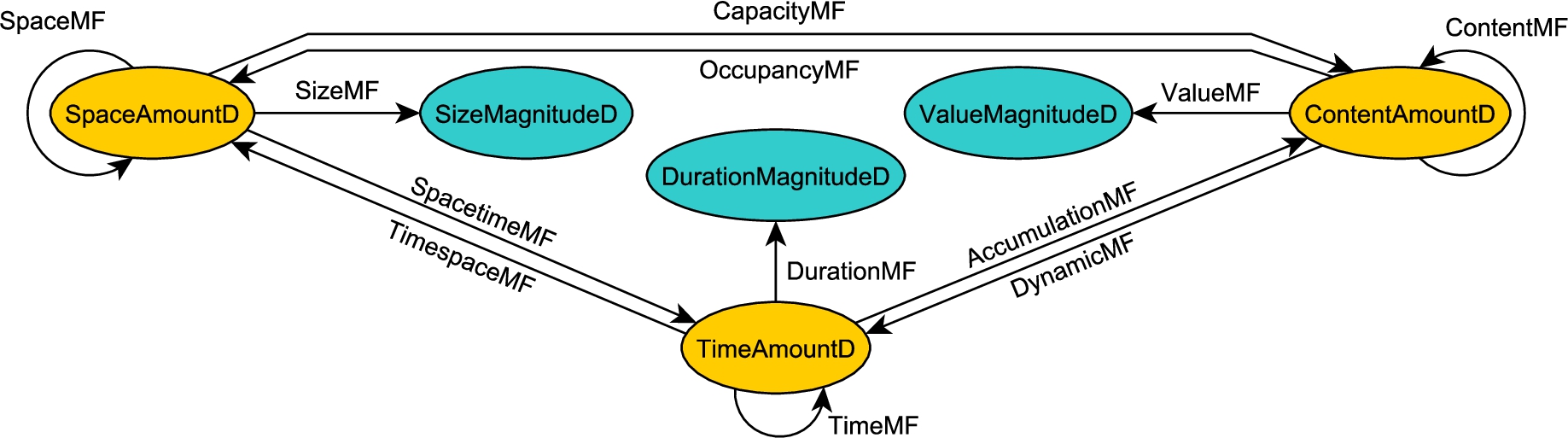
Extensivity triangle, showing possibilities of extensive measurement functions between three categories of quantity domains.

In the following, we discuss each of the measurement function classes using examples of geographic maps, nine of which are assembled in Fig. 4 and Fig. 5. These maps are all univariate, but since extensivity is induced at the measurement function level, the same principles apply to multivariate maps if for each variable a different function is assumed. We do not provide separate examples for the automorphisms since these can be explained by means of the examples for the other measurement function classes. Table 2 gives a preliminary overview of the twelve measurement function classes.

Fig. 4.

Examples of magnitude-of-amount measurements.

Fig. 5.

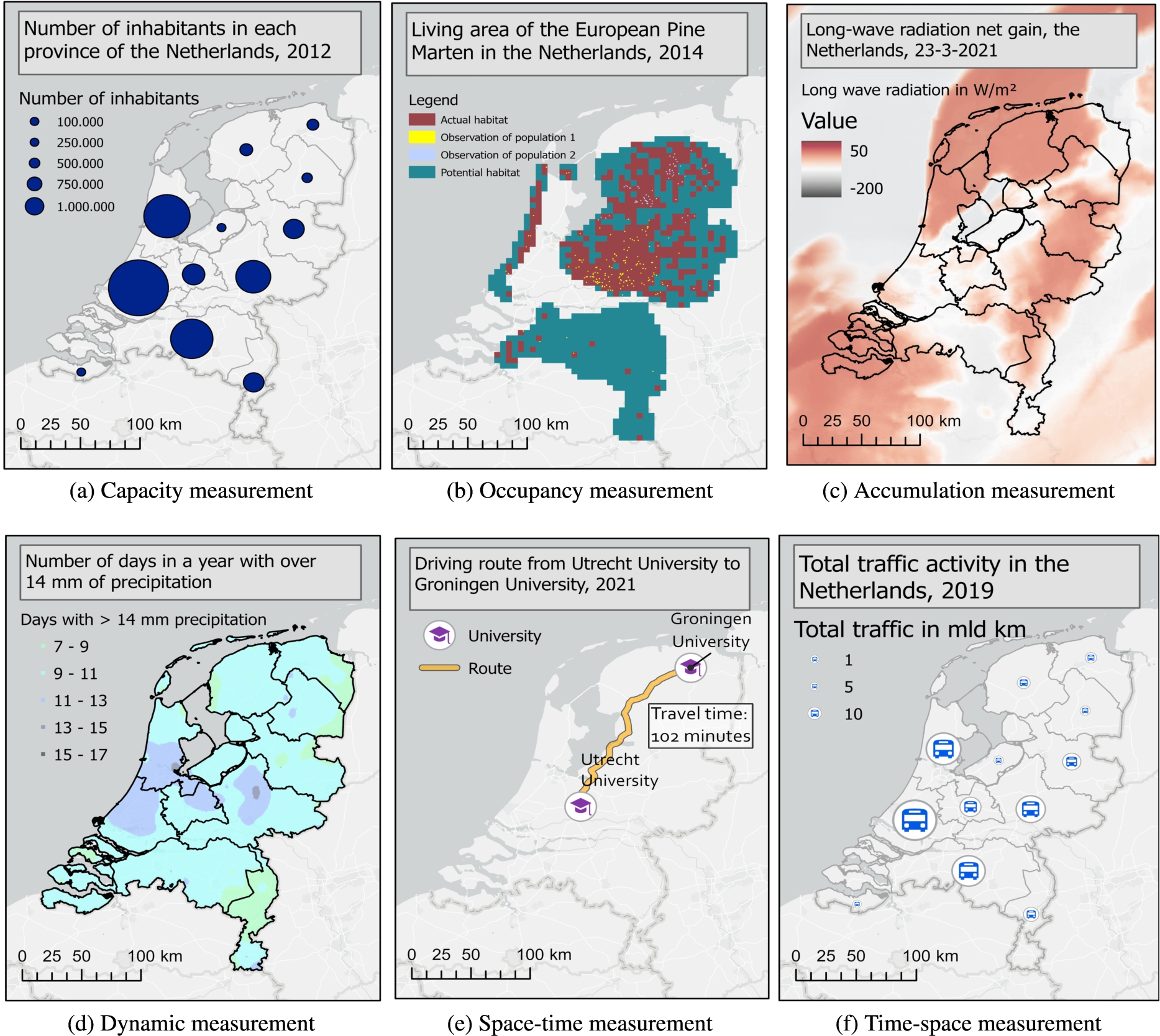
Examples of amount-of-amount measurements.

4.2. Magnitude-of-amount measurements

A MagnitudeOfAmountMF is a function that retrieves a magnitude from some amount. We distinguish three of these, namely SizeMF which measures from regions (amounts of space) to sizes (spatial magnitudes), DurationMF which measures from amounts of time to durations (temporal magnitudes), and ValueMF which measures from some other content amounts to other magnitudes, such as a count of objects, a monetary value, or a weight.

Functions in the SizeMF class yield spatial magnitudes from amounts of space. Figure 4(a) provides an example of size measurements. The map depicts the spatial sizes of the provinces of the Netherlands. Clearly the regions of the provinces do not overlap and are partially ordered. They form a lattice with an extensive mereology (regions can be part of one another). The amounts are related to their size magnitudes, which in turn are totally ordered. According to our definition of additivity, the sizes of the regions can be directly summed to infer the sizes of mergers, because the regions do not overlap.

Functions in the DurationMF class yield temporal magnitudes from amounts of time. Figure 4(b) shows the age of churches in the Netherlands that exist for at least 500 years. In this example, the periods of existence of each church overlap for at least the last 500 years, meaning for some time the churches exist at the same time. Just like with sizes, durations can be compared and be added up to derive the duration of existence of all churches. However, when summing up, overlaps need to be taken into account.

Functions in the ValueMF class yield magnitudes from amounts of content. For example, in Fig. 4(c), each bubble represents a magnitude of energy of an amount (a discrete collection) of wind turbines. Note that each bubble may contain multiple wind turbines which are implicit here. Another possible value measure would be the number of wind turbines in each cluster.

Table 2
Overview of geographic measurement function classes

Superclass Class Control Measure Example

MagnitudeOfAmountMF SizeMF SpaceAmount SizeMagnitude Europe area → Europe area size

DurationMF TimeAmount DurationMagnitude Length of a day in minutes

ValueMF ContentAmount ValueMagnitude Temperature in Celsius

AmountOfAmountMF (different cat.) CapacityMF SpaceAmount ContentAmount People in Europe

OccupancyMF ContentAmount SpaceAmount Area owned by local farmers

AccumulationMF TimeAmount ContentAmount Total precipitation in an hour

DynamicMF ContentAmount TimeAmount Years with olympic games

SpacetimeMF SpaceAmount TimeAmount Time of a train trip

TimespaceMF TimeAmount SpaceAmount Space traversed during a flight

AmountOfAmountMF (same cat.) SpaceMF SpaceAmount SpaceAmount Deforested area in a natural reserve

TimeMF TimeAmount TimeAmount Time of the day spent awake

ContentMF ContentAmount ContentAmount Amount of flour in a stack of pancakes

Superclass	Class	Control	Measure	Example
MagnitudeOfAmountMF	SizeMF	SpaceAmount	SizeMagnitude	Europe area → Europe area size
DurationMF	TimeAmount	DurationMagnitude	Length of a day in minutes
ValueMF	ContentAmount	ValueMagnitude	Temperature in Celsius
AmountOfAmountMF (different cat.)	CapacityMF	SpaceAmount	ContentAmount	People in Europe
OccupancyMF	ContentAmount	SpaceAmount	Area owned by local farmers
AccumulationMF	TimeAmount	ContentAmount	Total precipitation in an hour
DynamicMF	ContentAmount	TimeAmount	Years with olympic games
SpacetimeMF	SpaceAmount	TimeAmount	Time of a train trip
TimespaceMF	TimeAmount	SpaceAmount	Space traversed during a flight
AmountOfAmountMF (same cat.)	SpaceMF	SpaceAmount	SpaceAmount	Deforested area in a natural reserve
TimeMF	TimeAmount	TimeAmount	Time of the day spent awake
ContentMF	ContentAmount	ContentAmount	Amount of flour in a stack of pancakes

4.3. Amount-of-amount measurements

An AmountOfAmountMF measures an amount by using another amount as a control. For example, a population can be measured by controlling space and counting the individuals within this space. Also, the space they occupy can be found by measuring the spatial extents of the individuals. Note that the former and latter measurements are opposed to each other.23

²³
They correspond to the opposing arrows “capacity” and “occupancy” in Fig. 3.

We distinguish nine amount-of-amount measurement functions. Six of these are mappings between different amount categories, while three of these, namely SpaceMF, TimeMF, and ContentMF, are functions from amount domains to other domains in the same category (e.g. from hours to minutes).

Based on this, we define six subclasses of measurement functions, namely CapacityMF, OccupancyMF, AccumulationMF, DynamicMF, SpacetimeMF, and TimespaceMF, where an amount domain is extensive with respect to an amount domain of a different category.

A CapacityMF maps from a spatial amount to a content amount. Figure 5(a) shows the population amounts of each province (e.g. the ‘population of Utrecht’) which has a certain magnitude (e.g. 500,000). The population amounts themselves are measured with the regions as controls. For example, the population of Utrecht is measured with the region of the province of Utrecht as control. An OccupancyMF is the converse in the sense that it maps from a domain of content amounts to a domain of amounts of space that these contents ‘occupy’. Figure 5(b) shows e.g. the living areas of European pine martens in the Netherlands, which is the space these animals occupy.

An AccumulationMF maps from a domain of time amounts to a content amount domain. Resulting measurements are accumulations of content within an amount of time. Figure 5(c) shows the net gain of long-wave radiation over one day. For each point in the Netherlands, a magnitude is given of the net radiation gain or loss accumulation over a day. These magnitudes are understood as mappings from radiation content, which is controlled by some time period. The converse of the accumulation measurement is the DynamicMF, which maps from content amounts to temporal amounts. The example in Fig. 5(d) shows the amounts of days per region that have exceeded a threshold of >14 mm precipitation in a year.

A SpacetimeMF maps, as the name suggests, from a domain of amounts of space to some domain of amounts of time. Figure 5(e) shows the route from Utrecht University to Groningen University, along with an indication of how long traveling this route takes by car. Note that this indication is not just a duration magnitude, but also implies a finite interval in time in which someone actually traveled. A longer path implies a larger time interval. This notion of time is key to Hägerstrand’s Time Geography, which tells us that space accessibility is limited by temporal constraints (Hägerstrand, 1970). A TimespaceMF maps from amounts of time to amounts of space. Figure 5(f) shows the magnitudes of the amounts of traffic activity in 2019 in traveled kilometers. Note that these amounts are extensive with respect to amounts of time, so they can be summed up with the amounts of traffic activity in 2018 to result in the amount for two years.

An amount may need to be measured with another amount from the same category as control. For example, the churches in Fig. 4(b) are selected from a bigger set of churches based on whether they have existed over 500 years. Only the resulting sub-selection is shown in the map with corresponding duration magnitudes. It is also possible to measure with semantically different controls within the same category. For example, an amount of pets can be measured with an amount of households as control. In turn, the amount of pets can be a control for measuring the amount of mice caught by each pet. We refer to all these options as SpaceMF, TimeMF and ContentMF for measurement functions from and to respectively spatial, temporal and content amounts.

4.4. Automatically inferring measurement function classes

The membership of measurements to the twelve measurement function classes can be inferred by means of subsumption reasoning. We exemplify this with a subset of the classes in the GeoAMMO ontology. Specifically, these are the classes SpaceAmountD for domains of amounts of space, TimeAmountD for domains of amounts of time and ContentAmountD for content domains and classes for their corresponding amount elements, and the AccumulationMF and CapacityMF classes for measurement functions that map from respectively amounts of time and amounts of space to contents, also with corresponding measurement classes.

We illustrate the inference steps with a measurement scenario of the amount of births per year in Dutch municipalities. For this purpose, we defined data instances that encode the information given by the corresponding map data. To show how measurement function classes can be inferred from quantity classes, we did not specify the measurement function classes of measurement instances. We manually specified only the classes of quantities (based on their domains) as well as hasMeasure and hasControl relations between measurements and quantities. Using Protégé’s HermiT 1.4.3.456 reasoner, it becomes possible to automatically infer the class membership of measurement instances, as illustrated with the blue lines in Fig. 6. For example, since the function AmountsofBirthsMF is both additive and subtractive, it is also ExtensiveMF. Furthermore, since its element tuple Ams2021BirthsM (denoting the amount of births in Amsterdam in 2021) is controlled by a space amount and extensively measures some content amount, it can be classified as CapacityM. Furthermore, since it is also controlled by some time amount, it is also an AccumulationM.

Fig. 6.

Births in Amsterdam in 2021 as an example of inference of measurement function classes. Ovals are instances and rectangles are classes. Dotted lines denote class membership and blue lines denote automatically-inferred relations.

5. Discussion and conclusion

To better understand and to automate decisions on the applicability of arithmetic operations to spatial information, we have suggested that the concept of extensivity should be redefined as a formal property of a measurement function from one or more control quantity domains to a measure quantity domain. We have proposed an algebraic formalization of the underlying notions quantity, amount, magnitude, and additivity of a measurement function, and have proven theorems that correspond with our intuition about these concepts. In our theory, amounts appear as distinct standalone entities with an extensional mereology and with sum, difference and product operators in the form of a mathematical lattice. Magnitudes, in contrast, are linearly ordered scales that can be used to measure amounts. The notion of quantity is considered merely a generalization of these notions. In distinction to previous measurement theories, extensivity is defined as a relation between quantity domains and a measurement function. Furthermore, while extensivity is currently primarily used to describe the behavior of physical properties, like mass and volume, our model can be used to generalize the applicability of this concept across various domains of measurement and different cases of information aggregation relevant for geographic information.

Our definition of extensivity not only lifts the restrictions of a fixed range of properties that can be considered extensive, but also the reliance on system theory. We exchanged the notion of quantities extensive with respect to systems (Cohen et al., 2007) for a simpler notion of quantities with an extensional mereology, similar to Guizzardi (2010) and Gangemi et al. (2001). Furthermore, extending on our previous ideas (Scheider and Huisjes, 2019), we reused Sinton (1978)’s notion of measure and control to formally define extensivity with respect to various control domains within the categories time, space and content. This gives rise to an extensivity triangle as a more versatile and succinct model of extensivity that is directly applicable to various forms of geographic information. We deliberately limited our scope to geographic information in this article. We have tested our model by applying it to a range of map examples, which allowed us to systematically categorize measurements relevant for GIS into twelve classes of extensivity that can be distinguished in principle. The GeoAMMO ontology is usable for semantic enrichment of any form of quantity in geographic information, although its classes may need be made more specific for some purposes, e.g. when different kinds of content amounts or different kinds of intensive measurements need to be distinguished.

Regarding our formal model, future work should concentrate on three issues. One strand of research is about the formal properties of a measurement function. Intuitively, we would always expect that two different controls can exist that have the same measure. This means the measurement function is expected to be non-injective in the case of a magnitude measure. An example would be two different piles of sand with the same weight, or two lectures of the same duration. However, if the measure is also an amount, we would expect, in contrast, that the measurement function is injective, at least in many cases. So every quantity in the range of the function has only a single quantity in its domain. For example, two distinct amounts of sand are always contained in different amounts of space, even if they have the same weight magnitude. However, we also have counter examples (measurements of amounts that are not injective), like the measurement of a projected area given some region in three dimensions.

Second, we have not investigated ‘derived’ (composite and conjugate) quantities in the context of extensivity. These quantities are related to others via certain operations, captured by formal relations between quantity domains (Aameri et al., 2020). We have argued in this paper that extensive and intensive quantities should not be confused with such derived quantities. However, this warrants further research. We suspect that, while extensivity can be defined as a property of a measurement function, compositivity and conjugativity may be defined in terms of transformations between magnitude domains of particular kinds of amounts that are related themselves. An example of the former would be a transformation from population count to population density using the size of the region that is occupied by the population amount. The latter is about reverting this transformation by multiplying the density with area size.

And third, regarding our categorization of classes of extensivity, the content class is still a coarse container for many different kinds of geographic amounts. It could thus be further differentiated according to the core concept model of spatial information (Kuhn, 2012). For example, one can distinguish countable object-based amounts from measurable integrals of fields. It would be beneficial to study amounts and magnitudes in relation to Kuhn’s core concepts. For example, an amount of objects is bound to be atomic, which is not the case for a field amount. Furthermore, to make the model practically usable, the dependency of various arithmetic operations (like weighted average and sum) on the form of extensive and intensive quantities needs to be investigated (Scheider and Huisjes, 2019). Another area of research is to investigate the role of amounts in natural language processing, such as geo-analytical question answering (Xu et al., 2020). Future research should focus on developing conceptual modelling practices involving extensivity relations, testing our notion of extensivity on empirical data involving analyst behavior, and on exploring intensive and alternative types of quantities and relations.

Although we limited our focus to the domain of geographic information, we do not exclude the possibility that our theory can be used for, or at least adapted to, other domains as well. As mentioned by Simons (2013), there is a tendency to confuse quantities with numbers in the context of measurements, and this tendency is not limited to the domain of geographic information. Similarly, we believe our relational notion of extensive measurement may help clarify when statistical uses of sums are valid in arbitrary domains.

Footnotes

Acknowledgement

This work was supported by the European Research Council (ERC) under the European Union’s Horizon 2020 research and innovation programme (grant agreement no. 803498 (QuAnGIS)).

References

Aameri, B., Chui, C., Grüninger, M., Hahmann, T. & Ru, Y. (2020). The FOUnt ontologies for quantities, units, and the physical world. Applied Ontology, 15(3), 313–359. doi:10.3233/AO-200231.

Alberty, R.A. (1997). Legendre transforms in chemical thermodynamics. The Journal of Chemical Thermodynamics, 29(5), 501–516. doi:10.1006/jcht.1996.0171.

Balazs, A. (2008). International vocabulary of metrology-basic and general concepts and associated terms. Chemistry International, 25.

Campbell, N.R. (1920). Physics – the Elements. Cambridge: Univ. Press.

Canagaratna, S.G. (1992). Intensive and extensive: Underused concepts. Journal of Chemical Education, 69(12), 957. doi:10.1021/ed069p957.

Casati, R., Varzi, A.C., et al. (1999). Parts and Places: The Structures of Spatial Representation. Mit Press.

Centraal Bureau voor Statistiek. Kerncijfers Wijken en Buurten, 2012. https://www.cbs.nl/nl-nl/maatwerk/2011/48/kerncijfers-wijken-en-buurten-2012.

Centraal Bureau voor Statistiek. CBS gebiedsindelingen. https://www.cbs.nl/nl-nl/dossier/nederland-regionaal/geografische-data/cbs-gebiedsindelingen.

Centraal Bureau voor Statistiek. Rijksmonumenten. https://opendata.cbs.nl/statline/portal.html?_la=nl&_catalog=CBS&tableId=84775NED&_theme=423.

10.

Centraal Bureau voor Statistiek. Totale vervoersprestatie in Nederland; vervoerwijzen, regio’s. https://opendata.cbs.nl/statline/#/CBS/nl/dataset/84687NED/table?ts=1617881414400.

11.

Chrisman, N.R. (1998). Rethinking levels of measurement for cartography. Cartography and Geographic Information Systems, 25(4), 231–242. doi:10.1559/152304098782383043.

12.

Chrisman, N.R. (2002). Exploring Geographic Information Systems. New York: Wiley.

13.

Claramunt, C. & Jiang, B. (2001). An integrated representation of spatial and temporal relationships between evolving regions. Journal of Geographical Systems, 3(4), 411–428. doi:10.1007/s101090100066.

14.

Cohen, E.R., Cvitas, T., Frey, J., Holmstrom, B., Kuchitsu, K., Marquardt, R., Mills, I., Pavese, F., Quack, M., Stohner, J., Strauss, H., Takami, M. & Thor, A.J. (2007). Quantities, Units and Symbols in Physical Chemistry. Green Book: IUPAC.

15.

ESRI Nederland, Klimaateffectatlas, Rijksinstituut voor Volksgezondheid en Milieu. Netto langgolvige straling – KNMI (bèta). https://www.arcgis.com/home/item.html?id=2752ef4366d5486388efde9ce3fd75fc.

16.

ESRI Nederland, Rijksinstituut voor Volksgezondheid en Milieu. Netto langgolvige straling – KNMI (bèta). https://www.arcgis.com/home/item.html?id=61dc70b9664f4c3c9818427203abdd73.

17.

Gahegan, M. (2020). Fourth paradigm GIScience? Prospects for automated discovery and explanation from data. International Journal of Geographical Information Science, 34(1), 1–21. doi:10.1080/13658816.2019.1652304.

18.

Galton, A. & Mizoguchi, R. (2009). The water falls but the waterfall does not fall: New perspectives on objects, processes and events. Applied Ontology, 4(2), 71–107. doi:10.3233/AO-2009-0067.

19.

Gangemi, A., Guarino, N., Masolo, C. & Oltramari, A. (2001). Understanding top-level ontological distinctions. In OIS@ IJCAI.

20.

Gerstl, P. & Pribbenow, S. (1993). Midwinters, end games and bodyparts. In International Workshop on Formal Ontology-93 (pp. 251–260).

21.

Guarino, N., Welty, C., et al. (2000). Identity, unity, and individuality: Towards a formal toolkit for ontological analysis. In ECAI (Vol. 2000, pp. 219–223). Citeseer.

22.

Guizzardi, G. (2010). On the Representation of Quantities and their Parts in Conceptual Modeling. In FOIS (pp. 103–116).

23.

Hägerstrand, T. (1970). What about people in regional science? Papers of the Regional Science Association, 24, 7–21. doi:10.1111/j.1435-5597.1970.tb01464.x.

24.

Hey, A.J., Tansley, S., Tolle, K.M., et al. (2009). The Fourth Paradigm: Data-Intensive Scientific Discovery (Vol. 1). Redmond, WA: Microsoft Research.

25.

Hitzler, P., Krotzsch, M. & Rudolph, S. (2009). Foundations of Semantic Web Technologies. Chapman and Hall/CRC.

26.

Hölder, O. (1901). Die Axiome der Quantität und die Lehre Vom Mass. Teubner.

27.

Kocourek, R.A. (2018). Quantity. New Catholic Encyclopedia. https://www.encyclopedia.com/literature-and-arts/language-linguistics-and-literary-terms/language-and-linguistics/quantity .

28.

Kuhn, W. (2012). Core concepts of spatial information for transdisciplinary research. International Journal of Geographical Information Science, 26(12), 2267–2276. doi:10.1080/13658816.2012.722637.

29.

Lachmair, M., Ruiz Fernández, S., Moeller, K., Nuerk, H.-C. & Kaup, B. (2018). Magnitude or multitude – what counts? Frontiers in Psychology, 9, 522. doi:10.3389/fpsyg.2018.00522.

30.

Lowe, E.J. (1998). Entity, identity and unity. Erkenntnis, 48(2), 191–208. doi:10.1023/A:1005327718934.

31.

Luce, R.D. & Suppes, P. (2002). Representational measurement theory.

32.

Mannaerts, S.H. (2014). Extensive quantities in thermodynamics. European Journal of Physics, 35(3), 035017. doi:10.1088/0143-0807/35/3/035017.

33.

Masolo, C., Borgo, S., Gangemi, A., Guarino, N. & Oltramari, A. (2003). Ontology Library. WonderWeb Deliverable D18 (ver. 1.0, 31-12-2003). Technical report, Laboratory For Applied Ontology-ISTCCNR.

34.

Nationale EnergieAtlas. Windturbines. https://www.nationaleenergieatlas.nl/kaarten.

35.

Padmanabhan, R. & Rudeanu, S. (2008). Axioms for Lattices and Boolean Algebras. World Scientific.

36.

Plewe, B.S. (2019). A case for geographic masses. In 14th International Conference on Spatial Information Theory (COSIT 2019). Schloss Dagstuhl-Leibniz-Zentrum Fuer Informatik.

37.

Probst, F. (2008). Observations, measurements and semantic reference spaces. Applied Ontology, 3(1–2), 63–89. doi:10.3233/AO-2008-0046.

38.

Redlich, O. (1970). Intensive and extensive properties. Journal of Chemical Education, 47(2), 154. doi:10.1021/ed047p154.2.

39.

Rijgersberg, H., Van Assem, M. & Top, J. (2013). Ontology of units of measure and related concepts. Semantic Web, 4(1), 3–13. doi:10.3233/SW-2012-0069.

40.

Rijksinstituut voor Volksgezondheid en Milieu. Genetische structuur van de Boommarter populatie (Martes martes). https://data.overheid.nl/dataset/abc85851-cede-4ddd-bc4c-cb69ad99b331.

41.

Ru, Y. & Gruninger, M. (2017). Parts Unknown: Mereologies for Solid Physical Objects. In JOWO.

42.

Scheider, S. & de Jong, T. (2022). A conceptual model for automating spatial network analysis. Transactions in GIS, 26.

43.

Scheider, S. & Huisjes, M.D. (2019). Distinguishing extensive and intensive properties for meaningful geocomputation and mapping. International Journal of Geographical Information Science, 33(1), 28–54. doi:10.1080/13658816.2018.1514120.

44.

Simons, P. (2013). Density, angle, and other dimensional nonsense: How not to standardize quantity. In Johanssonian Investigations (pp. 516–534). De Gruyter.

45.

Sinton, D. (1978). The inherent structure of information as a constraint to analysis: Mapped thematic data as a case study. In Harvard Papers on Geographic Information Systems.

46.

Steinberg, M.D., Schindler, S. & Keil, J.M. (2016). Use cases and suitability metrics for unit ontologies. In OWL: Experiences and Directions–Reasoner Evaluation (pp. 40–54). Springer.

47.

Stevens, S.S., et al. (1946). On the Theory of Scales of Measurement.

48.

Suppes, P. & Zinnes, J.L. (1962). Basic measurement theory. In Handbook of Mathematical Psychology (Vol. 1).

49.

Talmy, L. (1978). The relation of grammar to cognition–a synopsis. American Journal of Computational Linguistics, 16–26.

50.

Tolman, R.C. (1917). The measurable quantities of physics. Physical Review, 9(3), 237–253.

51.

Wright, J.K. (1955). “Crossbreeding” geographical quantities. Geographical Review, 45(1), 52–65. doi:10.2307/211729.

52.

Xu, H., Hamzei, E., Nyamsuren, E., Kruiger, H., Winter, S., Tomko, M. & Scheider, S. (2020). Extracting interrogative intents and concepts from geo-analytic questions. AGILE: GIScience Series, 1, 1–21.