Junction of quasi-stationary ferromagnetic thin films

Abstract

In this paper we study the asymptotic behavior of the solutions of time dependent micromagnetism problem in a multi-domain consisting of two joined ferromagnetic thin films. We distinguish different regimes depending on the limit of the ratio between the small thickness of the two films.

Keywords

micromagnetics variational problem thin films Landau–Lifshitz equation

1. Introduction

Ferromagnetic behavior, in particular the presence of spontaneous magnetization even in the absence of an applied magnetic field, can be examined by the theory started by Weiss in 1907 and perfectioned by Landau and Lifshitz in 1935 (see [35] and for a modern analysis see [5]). It is proposed that, under suitable conditions, in particular when the temperature is below a critical point (the so called Curie’s temperature, characteristic of the material), a ferromagnetic body breaks up into uniformly magnetized region (Weiss domains) separated by thin transition layers (Bloch wall), even in the absence of any applied magnetic field. Then, the phenomena can be described by a magnetization field M, defined on the domain Ω in which the material is confined, which on a microscopic scale has a fixed modulus $| M | = m = const$ and variable orientation, because of the presence of a strong molecular field. So, the system can be studied through the functional representing its magnetic energy. This energy consists in several terms: the so called exchange energy, which contains the space derivative of M and is peculiar to ferromagnetic behavior, a term corresponding to magnetic anisotropy, and another one depending on the magnetic field H, which is related to M via the equations of magnetostatic.

More precisely, assume the body is homogeneous and has a uniform temperature. Then the magnetic induction B, the magnetic field H and the magnetization M are connected by: the relation $B = H (M) + \overline{M}$ where $\overline{M}$ is the extension by zero of M outside Ω; the static Maxwell equation and the magnetostatic equation (Faraday law): $\{\begin{matrix} \nabla \times H (M) = 0, \\ div (H (M) + \overline{M}) = div (B) = 0 . \end{matrix}$ (1.1)

So the steady state configuration of M corresponds to a minimum of the following functional E representing the magnetic energy: $\{\begin{matrix} E (M) = \int_{Ω} (| D M |^{2} + \frac{1}{2} {| H (M) |}^{2} + φ (M)) d x \\ subject to conditions (1.1), \end{matrix}$ (1.2) where E is obtained by summing up the exchange energy $E^{exc} = \int_{Ω} | D M |^{2} d x$ , the magnetostatic energy $E^{mag} = \int_{Ω} | H (M) |^{2} d x$ , which is related to M via equation of magnetostatic, and the anisotropy energy $E^{an} = \int_{Ω} φ (M) d x$ .

Existence of the minimizers of E is proved in [39]; here the author showed that the total magnetic energy as a functional of M is convex, coercive and lower-semicontinuous in Sobolev space $H^{1}$ , hence the corresponding minimization problem as at least one solution. Of course this is not unique, in general, because of the non-convexity of the constraint $| M | = m$ . Regularity results about these minimizers are proved in [6,30] and [39].

Gioia and James in [27] study the asymptotic behavior arbitrary-shaped very thin films of small thickness. They analyze “rescaled energies”. So they prove that the thickness of the film imports an artificial anisotropy which disfavours out of plane magnetization. Moreover, the limiting energy is completely local, that is to say the magnetostatic equation which contains the magnetization m in the original problem, disappears from the limiting one. Problems of dimension reduction in magnetostatic were treated by several authors. A pioneering work is the paper of Stoner and Wohlfarth (1948). A rigorous treatment in this case was given by De Simone [16]. Carbou treated the case of magnetic wire in [9,10] and the case of thin films again in [7]. Other regimes are considered in [18] and [17] in the case of the films. In [23] and [24] Gaudiello and Hadiji studies the behavior of minimizers of Problem (1.2) in a multidomain. More precisely, in [23] Gaudiello and Hadiji, study the free energy of two joined ferromagnetic thin films distinguishing different regimes depending on the limit of the ratio between the small thickness of the two films. In what concerns the study of a ferroelectric materials see also [25]. See [20,22,26] for junction 3D–1D and [21] for junction 1D–1D.

When the body is isotropic, one can assume $φ (M) = 0$ . In this case the quasi-stationary model situation is governed by Landau–Lifshitz’s equation (see [8,35]) $\frac{\partial M}{\partial t} + M \land \frac{\partial M}{\partial t} = 2 M \land (Δ M + H (M))$ (1.3) subject to conditions (1.1).

The existence result for this problem is proved, in a more general case, in [39] (see Theorem 2) and in [8] (see Sections 3 and 5), see also [3] and [29]. We observe (see [8] and [39]) that the corresponding configuration satisfies an energy estimate.

Then Carbou in [7], as Gioia and James [27] in the stationary case, studies the limit behavior of the isotropic ferromagnetic films when the thicknesses goes to zero, in the quasi stationary case. Other similar problems are studied by Ammari et al. [3]. The homogenization of the Landau–Lifshitz equation in periodically perforated domain was studied in [37]. For related problems see also [1,2,15,28,34].

In this work we study, as Gaudiello and Hadiji in the stationary case (see [23]), the limit behavior of a system governed by Landau–Lifshitz equation, in an isotropic ferromagnetic multi-domain consisting of two joined thin films when the thicknesses goes to zero, by using, also, some ideas contained in [7,23] and [36].

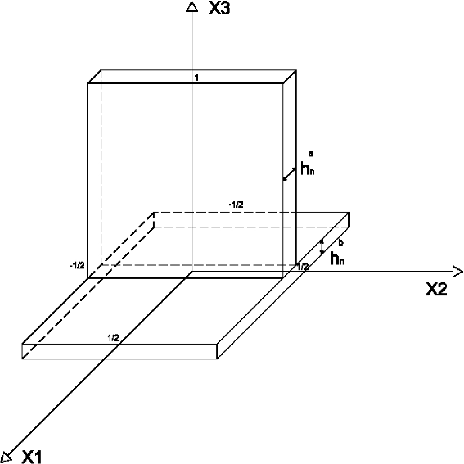
More precisely, for every $n \in N$ , let $\begin{matrix} Ω_{n}^{a} = (] - \frac{h_{n}^{a}}{2}, \frac{h_{n}^{a}}{2} [\times] - \frac{1}{2}, \frac{1}{2} [\times [0, 1 [), Ω_{n}^{b} = ({] - \frac{1}{2}, \frac{1}{2} [}^{2} \times] - h_{n}^{b}, 0 [), \\ Ω_{n} = Ω_{n}^{a} \cup Ω_{n}^{b}, \end{matrix}$ (1.4) be a 3D ferromagnetic multidomain consisting of two orthogonal joined films, as in Fig. 1, with small thicknesses ${h_{n}^{a}}_{n \in N}, {h_{n}^{b}}_{n \in N} \subset] 0, 1 [$ such that $lim_{n} h_{n}^{a} = 0 = lim_{n} h_{n}^{b}, lim_{n} \frac{h_{n}^{b}}{h_{n}^{a}} = q \in [0, + \infty] .$ (1.5) (For instance, such structure appears as a component of a rotor of a permanent magnetic synchronous micro-machine, see Irudayarai and Emadi [32].)

Fig. 1.

$Ω_{n}$ .

Then, for any fixed $T > 0$ , the aim of our paper is to study the asymptotic behavior as n diverges, of the following problem: $\{\begin{matrix} | M_{n} (x) | = 1 & in Ω_{n}, \\ \frac{\partial M_{n}}{\partial t} + M_{n} \land \frac{\partial M_{n}}{\partial t} = 2 M_{n} \land (Δ M_{n} + H (M_{n})) & in Ω_{n} \times] 0, T [, \\ M_{n} (0, x) = M_{0_{n}} (x) & in Ω_{n}, \\ H (M_{n}) and M_{n} linked by (1.1) for every t, \end{matrix}$ (1.6) where $| M_{0_{n}} (x) | = 1$ in $Ω_{n}$ .

If $q \in] 0, + \infty [$ (i.e. $h_{n}^{b} ≃ h_{n}^{a}$ ), assuming that the initial energy is an $O (h_{n}^{a})$ , we show that the solutions of (1.6) converge in mean square, for every t, up to a subsequence, to solutions of the following limit problem, “morally” defined only on two perpendicular sections $\{\begin{matrix} \frac{\partial μ^{a}}{\partial t} + μ^{a} \land \frac{\partial μ^{a}}{\partial t} = 2 μ^{a} \land (Δ μ^{a} - (μ^{a}, e_{1}) e_{1}) in] 0, T [\times] - \frac{1}{2}, \frac{1}{2} [\times] 0, 1 [, \\ q \frac{\partial μ^{b}}{\partial t} + q (μ^{b} \land \frac{\partial μ^{b}}{\partial t}) = 2 q μ^{b} \land (Δ μ^{b} - (μ^{b}, e_{3}) e_{3}) in] 0, T [\times {] - \frac{1}{2}, \frac{1}{2} [}^{2}, \\ μ^{a} (0, x_{2}, x_{3}) = μ_{0}^{a} (x) in] - \frac{1}{2}, \frac{1}{2} [\times] 0, 1 [, \\ μ^{b} (0, x_{1}, x_{2}) = μ_{0}^{b} (x) in {] - \frac{1}{2}, \frac{1}{2} [}^{2}, \\ μ^{a} (t, x_{2}, 0) = μ^{b} (t, 0, x_{2}) for x_{2} in] - \frac{1}{2}, \frac{1}{2} [and t in [0, T], \\ | μ^{a} | = 1 for x in] - \frac{1}{2}, \frac{1}{2} [\times] 0, 1 [, | μ^{b} | = 1 for x in {] - \frac{1}{2}, \frac{1}{2} [}^{2}, \end{matrix}$ (1.7) where $μ = (μ^{a}, μ^{b})$ is a pair of coupled magnetic fields acting on to a couple of perpendicular surfaces. We explicitly observe that the coupling between the two 2D problems is given by the junction condition $μ^{a} (\cdot, x_{2}, 0) = μ^{b} (\cdot, 0, x_{2})$ , for $x_{2}$ in $] - \frac{1}{2}, \frac{1}{2} [$ . Moreover, $μ_{0}^{a}$ and $μ_{0}^{b}$ in (1.7) are limits in mean square of the initial data $M_{0_{n}}$ .

Eventually we prove that if the initial energy is an $o (h_{n}^{a})$ then the converging subsequences of $M_{n}$ converge in mean square, for every t, to $μ = (0, 1, 0)$ or to $μ = (0, - 1, 0)$ .

We note that this problem is completely local. The cases $q = 0$ and $q = + \infty$ were studied in [14]. Here we proved that if $q = 0$ (i.e. $h_{n}^{b} ≪ h_{n}^{a}$ ) the limit problem reduces to a 2D local problem in a vertical thin film losing the junction condition (see [14], Theorem 3.1). Analogously, if $q = + \infty$ (i.e. $h_{n}^{a} ≪ h_{n}^{b}$ ) the limit problem reduces to a 2D local problem in an horizontal thin film (see [14], Theorem 3.2).

We obtain our result by reformulating the problem in a fixed domain $Ω = Ω^{a} \cup Ω^{b}$ , with $Ω^{a} =] - \frac{1}{2}, \frac{1}{2} [^{2} \times] 0, 1 [$ and $Ω^{b} =] - \frac{1}{2}, \frac{1}{2} [^{2} \times] - 1, 0 [$ , through appropriate rescalings of the kind proposed by Ciarlet and Destuynder [11], and by using the main ideas of Γ-convergence method introduced by De Giorgi [13].

The paper is organized as follows. Section 2 is devoted to give a precise mathematical statement of the problem and some preliminary results. In Section 3, we give the main results. In Section 4 we give a compactness result. In Section 5 we study the behavior of magnetostatic energy. In Section 6 we prove the main results.

2. Statement of the problem and preliminary results

2.1. Preliminary notations and weak formulation of (1.6) and (1.7)

Let $x = (x_{1}, x_{2}, x_{3})$ denote the generic point of $R^{3}$ . If $a, b, c \in R^{3}$ , then $(a ∣ b ∣ c)$ denotes the $3 \times 3$ real matrix having $a^{T}$ as first column $b^{T}$ as second column and $c^{T}$ as third column. In according with this notation if $v : A \subset R^{3} \to R^{3}$ then $D v$ denotes the $3 \times 3$ real matrix $(D_{x_{1}} v ∣ D_{x_{2}} v ∣ D_{x_{3}} v)$ , where $D_{x_{i}} v \in R^{3}$ , $i = 1, 2, 3$ , stands for the derivative of v with respect to $x_{i}$ . Let $S^{2}$ be the unit sphere of $R^{3}$ .

Let B be a rectangle containing $\overline{Ω_{n}}$ , for every $n \in N$ , for instance let $B =] - 1, 1 [^{2} \times] - 2, 2 [$ . Let us consider the space $U = {U \in L_{loc}^{1} (R^{3}) : U \in L^{2} (B), D U \in {(L^{2} (R^{3}))}^{3}, \int_{B} U d x = 0} .$ (2.1) It is easy to prove that $U$ is contained in $L_{loc}^{2} (R^{3})$ and it is an Hilbert space with the inner product $(U, V) = \int_{R^{3}} D U D V d x + \int_{B} U V d x$ . Moreover, from Poincaré–Wirtinger inequality it follows that a norm on $U$ equivalent to ${(U, U)}^{\frac{1}{2}}$ is given by ${(\int_{R^{3}} | D U |^{2} d x)}^{\frac{1}{2}}$ . To reformulate conditions (1.1), related to Eq. (1.3), as usual let us introduce $U_{M}$ , the scalar magnetostatic potential, which satisfies the equation $div (- D U_{M} + \overline{M}) = 0$ , where $\overline{M}$ denotes the zero extension of M outside $Ω_{n}$ . Posed $H = - D U_{M}$ , obviously, we obtain $\nabla \times H (M) = 0$ and then conditions (1.1). Let $M \in L^{2} (Ω_{n}, R^{3})$ then the following problem $\{\begin{matrix} U_{M} \in U, \\ \int_{R^{3}} D U_{M} D U = \int_{Ω_{n}} M D U d x \forall U \in U, \end{matrix}$ (2.2) admits a unique solution $U_{M} \in U$ . This solution is characterized as the unique minimizer of the following problem: $min {\frac{1}{2} \int_{R^{3}} | D U - \overline{M} |^{2} d x : U \in U},$ (2.3) where as usual $\overline{M}$ denotes the zero extension of M in $R^{3} ∖ Ω_{n}$ . Moreover, $U_{M} \in H^{1} (R^{3})$ up to an additive constant, see [33]. Then a weak formulation of the Landau–Lifshitz equation (1.6) in our case is the following.

Fixed $M_{0_{n}} \in H^{1} (Ω_{n}, S^{2})$ ( $U_{0_{n}} \in U$ being the corresponding solution of Problem (2.2)), find $M_{n}$ which satisfies $\{\begin{matrix} M_{n} \in L^{\infty} (0, T; H^{1} (Ω_{n}, R^{3})) \cap C ([0, T]; L^{2} (Ω_{n}, R^{3})), \\ | M_{n} | = 1 a.e. in [0, T] \times Ω_{n}, \frac{\partial M_{n}}{\partial t} \in L^{2} (0, T; L^{2} (Ω_{n}, R^{3})), \\ \forall χ \in D (0, T) and ψ \in H^{1} (Ω_{n}, R^{3}), \\ \int_{0}^{T} \int_{Ω_{n}} (\frac{\partial M_{n}}{\partial t} + M_{n} \land \frac{\partial M_{n}}{\partial t}) χ ψ d x d t = - 2 \int_{0}^{T} \int_{Ω_{n}} \sum_{i = 1}^{3} (M_{n} \land D_{x_{i}} M_{n}) (D_{x_{i}} ψ) χ d x d t \\ - 2 \int_{0}^{T} \int_{Ω_{n}} (M_{n} \land D U_{M_{n}}) χ ψ d x d t, \\ M_{n} (0, x) = M_{0_{n}} (x) a.e. x in Ω_{n}, \\ U_{M_{n}} and M_{n} linked by (2.2) for every t \in [0, T] . \end{matrix}$ (2.4) Now, we give an existence result for Problem (2.4) slightly adapting results contained in [8] and [39].

Theorem 2.1.

Let $M_{0_{n}} \in H^{1} (Ω_{n}, S^{2})$ . Then there exists at least a weak solution of Problem ( 2.4 ). Moreover, it satisfies the following energy estimate: $E (M_{n} (t, \cdot)) + \int_{0}^{t} {∥ \frac{\partial M_{n}}{\partial t} ∥}_{{(L^{2} (Ω_{n}))}^{3}}^{2} d s ⩽ E (M_{n} (0, \cdot)) = E (M_{0_{n}}) for a.e. t \in [0, T] .$ (2.5)

Proof.

By a density like argument (for instance see [31], Lemma 1.9, p. 39, and also [19]), Problem (2.4) is equivalent to problem $\{\begin{matrix} M_{n} \in L^{\infty} (0, T; H^{1} (Ω_{n}, R^{3})) \cap C ([0, T]; L^{2} (Ω_{n}, R^{3})), \\ | M_{n} | = 1 a.e. in [0, T] \times Ω_{n}, \frac{\partial M_{n}}{\partial t} \in L^{2} (0, T; L^{2} (Ω_{n}, R^{3})) \\ \forall ϕ \in D (] 0, T [\times \overline{Ω_{n}}, R^{3}), \\ \int_{0}^{T} \int_{Ω_{n}} (\frac{\partial M_{n}}{\partial t} + M_{n} \land \frac{\partial M_{n}}{\partial t}) ϕ d x d t = - 2 \int_{0}^{T} \int_{Ω_{n}} \sum_{i = 1}^{3} (M_{n} \land D_{x_{i}} M_{n}) (D_{x_{i}} ϕ) d x d t \\ - 2 \int_{0}^{T} \int_{Ω_{n}} (M_{n} \land D U_{M_{n}}) ϕ d x d t, \\ M_{n} (0, x) = M_{0_{n}} (x) a.e. x in Ω_{n}, \\ U_{M_{n}} and M_{n} linked by (2.2) for every t \in [0, T], \end{matrix}$ (2.6) by choosing as test functions $ϕ = χ ψ$ with $χ \in D (0, T)$ and $ψ \in H^{1} (Ω_{n}, R^{3})$ . In [8] and [39] the existence of a solution $M_{n} \in L^{\infty} (0, T; H^{1} (Ω_{n}, R^{3}))$ such that $\frac{\partial M_{n}}{\partial t} \in L^{2} (0, T; L^{2} (Ω_{n}, R^{3}))$ , with $| M_{n} | = 1$ a.e. in $[0, T] \times Ω_{n}$ of Problem (2.6) and estimate (2.5) are proved. Moreover, by Proposition 23.23 in [40] (see also [12]) we have that $M_{n} \in C ([0, T]; L^{2} (Ω_{n}, R^{3}))$ . Consequently, $M_{n} (0, x) = M_{0_{n}} (x)$ is well defined and $M (t, x)$ is well defined for every $t \in [0, T]$ and for a.e. x in $Ω_{n}$ , so we get the thesis. □

Moreover, we pose, for every $t \in [0, T]$ $E (M_{n} (t, \cdot)) = \int_{Ω_{n}} {| D M_{n} (t, x) |}^{2} d x + \frac{1}{2} \int_{R^{3}} {| D U_{M_{n}} (t, x) |}^{2} d x,$ the magnetic energy (i.e. the sum of the exchange and magnetostatic energies). We observe that $E (M_{n} (0, \cdot)) = \int_{Ω_{n}} | D M_{0_{n}} |^{2} d x + \frac{1}{2} \int_{R^{3}} | D U_{M_{0_{n}}} |^{2} d x .$ Moreover, we will denote $E (M_{n} (0, \cdot)) = E (M_{0_{n}}) .$

Now we want to give a variational formulation of (1.7).

To formulate our result precisely it is necessary to look at the 2D Problem (1.7) as a 3D problem defined on the domain $Ω = Ω^{a} \cup Ω^{b}$ . To this aim let consider $ψ = (ψ^{a}, ψ^{b}) \in H^{1} ({0} \times] - \frac{1}{2}, \frac{1}{2} [\times] 0, 1 [, R^{3}) \times H^{1} (] - \frac{1}{2}, \frac{1}{2} [^{2} \times {0}, R^{3})$ such that $ψ^{a} (0, x_{2}, 0) = ψ^{b} (0, x_{2}, 0)$ for $x_{2}$ in $] - \frac{1}{2}, \frac{1}{2} [$ in the trace sense.

Let us suppose that $ψ^{a}$ is extended on $Ω^{a}$ so that it does not depend on $x_{1}$ . Similarly, let us suppose that $ψ^{b}$ is extended on $Ω^{b}$ so that it does not depend on $x_{3}$ . These extensions will be denoted by the same symbol. Under this notation makes sense to write $ψ^{a} (x_{1}, x_{2}, 0) = ψ^{b} (0, x_{2}, x_{3})$ for $x_{2}$ a.e. in $] - \frac{1}{2}, \frac{1}{2} [$ . In this sense, we can introduce the following space $\begin{array}{rclr} W & = & {ψ = (ψ^{a}, ψ^{b}) \in H^{1} (Ω^{a}, R^{3}) \times H^{1} (Ω^{b}, R^{3}) : \\ ψ^{a} is constant in x_{1}, ψ^{b} is constant in x_{3}, \\ ψ^{a} (x_{1}, x_{2}, 0) = ψ^{b} (0, x_{2}, x_{3}) for x_{2} a.e. in] - \frac{1}{2}, \frac{1}{2} [} . & (2.7) \end{array}$ Moreover, we can pose $M = W \cap {H^{1} (Ω^{a}, S^{2}) \times H^{1} (Ω^{b}, S^{2})},$ (2.8) which explicitly takes into account the condition $| ψ | = 1$ and $L^{\infty} (0, T; M) = {μ \in L^{\infty} (0, T; H^{1} (Ω^{a}, R^{3}) \times H^{1} (Ω^{b}, R^{3})) : a.e. t \in [0, T], μ (t, \cdot) \in M} .$ (2.9) Then, the equivalent 3D variational formulation of Problem (1.7) is the following one: $\{\begin{matrix} μ = (μ^{a}, μ^{b}) \in L^{\infty} (0, T; M) \cap C ([0, T]; L^{2} (Ω^{a}, R^{3}) \times L^{2} (Ω^{b}, R^{3})), \\ \frac{\partial μ}{\partial t} \in L^{2} (0, T; L^{2} (Ω^{a}, R^{3}) \times L^{2} (Ω^{b}, R^{3})), \\ \forall χ \in D (0, T) and ψ = (ψ^{a}, ψ^{b}) \in W, \\ \int_{0}^{T} \int_{Ω^{a}} (\frac{\partial μ^{a}}{\partial t} + μ^{a} \land \frac{\partial μ^{a}}{\partial t}) χ ψ^{a} d x d t + q \int_{0}^{T} \int_{Ω^{b}} (\frac{\partial μ^{b}}{\partial t} + μ^{b} \land \frac{\partial μ^{b}}{\partial t}) χ ψ^{b} d x d t \\ = - 2 \int_{0}^{T} \int_{Ω^{a}} \sum_{i = 2}^{3} μ^{a} \land \frac{\partial μ^{a}}{\partial x_{i}} \frac{\partial ψ^{a}}{\partial x_{i}} χ d x d t - 2 q \int_{0}^{T} \int_{Ω^{b}} \sum_{i = 1}^{2} μ^{b} \land \frac{\partial μ^{b}}{\partial x_{i}} \frac{\partial ψ^{b}}{\partial x_{i}} χ d x d t \\ - 2 \int_{0}^{T} \int_{Ω^{a}} μ^{a} \land (μ^{a}, e_{1}) e_{1} χ ψ^{a} d x d t - 2 q \int_{0}^{T} \int_{Ω^{b}} μ^{b} \land (μ^{b}, e_{3}) e_{3} χ ψ^{b} d x d t, \\ μ^{a} (0, x) = μ_{0}^{a} (x) a.e. x in Ω^{a}, \\ μ^{b} (0, x) = μ_{0}^{b} (x) a.e. x in Ω^{b}, \\ μ_{0} = (μ_{0}^{a}, μ_{0}^{b}) \in M . \end{matrix}$ (2.10) To Problem (2.10), for a.e. $t \in [0, T]$ , the following energy will be associated, $E_{q} (t) + \int_{0}^{t} {∥ \frac{\partial μ^{a}}{\partial t} ∥}_{(L^{2} {({0} \times] - \frac{1}{2}, \frac{1}{2} [\times] 0, 1 [))}^{3}}^{2} d s + q \int_{0}^{t} {∥ \frac{\partial μ^{b}}{\partial t} ∥}_{(L^{2} {(] - \frac{1}{2}, \frac{1}{2} [^{2} \times {0}))}^{3}}^{2} d s,$ (2.11) where $\begin{array}{rclr} E_{q} (t) & = & \int_{{0} \times] - \frac{1}{2}, \frac{1}{2} [\times] 0, 1 [} {| D μ^{a} |}^{2} d x_{2} d x_{3} + q \int_{] - \frac{1}{2}, \frac{1}{2} [^{2} \times {0}} {| D μ^{b} |}^{2} d x_{1} d x_{2} \\ + \frac{1}{2} \int_{{0} \times] - \frac{1}{2}, \frac{1}{2} [\times] 0, 1 [} {| μ_{1}^{a} |}^{2} d x_{2} d x_{3} + \frac{1}{2} q \int_{] - \frac{1}{2}, \frac{1}{2} [^{2} \times {0}} {| μ_{3}^{b} |}^{2} d x_{1} d x_{2} . & (2.12) \end{array}$ Here, the term $E_{q}^{exc} (t) = \int_{{0} \times] - \frac{1}{2}, \frac{1}{2} [\times] 0, 1 [} {| D μ^{a} |}^{2} d x_{2} d x_{3} + q \int_{] - \frac{1}{2}, \frac{1}{2} [^{2} \times {0}} {| D μ^{b} |}^{2} d x_{1} d x_{2},$ (2.13) can be considered an exchange energy and the term $E_{q}^{mag} (t) = \frac{1}{2} \int_{{0} \times] - \frac{1}{2}, \frac{1}{2} [\times] 0, 1 [} {| μ_{1}^{a} |}^{2} d x_{2} d x_{3} + \frac{1}{2} q \int_{] - \frac{1}{2}, \frac{1}{2} [^{2} \times {0}} {| μ_{3}^{b} |}^{2} d x_{1} d x_{2},$ (2.14) can be considered the equivalent of a magnetostatic energy.

Now, we give a density result (see also [23] and Lemma 4.10 in [36]).

Let us pose $S = {0} \times [- \frac{1}{2}, \frac{1}{2}] \times [0, 1] \cup {[- \frac{1}{2}, \frac{1}{2}]}^{2} \times {0}$ . We denote the space of the Lipschitz continuous functions on S by $L$ . In the following with slight abuse of notation, we will continue to denote with $L$ the space of functions ψ on Ω such that ψ restricted to S is in $L$ , ψ is constant in $x_{1}$ in $Ω^{a}$ and is constant in $x_{3}$ in $Ω^{b}$ . Proposition 2.2.

Let $W$ be the space defined in ( 2.7 ). Then, $L$ is dense in $W$ .

Proof.

Let $(ψ^{a}, ψ^{b}) \in W$ . The goal is to find a sequence ${(ψ_{n}^{a}, ψ_{n}^{b})}_{n \in N} \subset L$ such that $\begin{array}{rclr} (ψ_{n}^{a}, ψ_{n}^{b}) \to (ψ^{a}, ψ^{b}) \\ strongly in H^{1} ({0} \times] - \frac{1}{2}, \frac{1}{2} [\times] 0, 1 [, R^{3}) \times H^{1} ({] - \frac{1}{2}, \frac{1}{2} [}^{2} \times {0}, R^{3}) & (2.15) \end{array}$ as n diverges.

We prove that it is possible to choose $(ψ_{n}^{a}, ψ_{n}^{b})$ such that $\begin{array}{rclr} {(ψ_{n}^{a}, ψ_{n}^{b}) \in C^{1} ({0} \times [- \frac{1}{2}, \frac{1}{2}] \times [0, 1], R^{3}) \times C ({[- \frac{1}{2}, \frac{1}{2}]}^{2} \times {0}, R^{3}) : \\ ψ_{n}^{b} |_{[- \frac{1}{2}, 0] \times [- \frac{1}{2}, \frac{1}{2}] \times {0}} \in C^{1} ([- \frac{1}{2}, 0] \times [- \frac{1}{2}, \frac{1}{2}] \times {0}, R^{3}), \\ ψ_{n}^{b} |_{[0, \frac{1}{2}] \times [- \frac{1}{2}, \frac{1}{2}] \times {0}} \in C^{1} ([0, \frac{1}{2}] \times [- \frac{1}{2}, \frac{1}{2}] \times {0}, R^{3}), \\ ψ_{n}^{a} (0, x_{2}, 0) = ψ_{n}^{b} (0, x_{2}, 0) for x_{2} in] - \frac{1}{2}, \frac{1}{2} [} . & (2.16) \end{array}$ To this aim, we begin by splitting $ψ^{b}$ in the odd part and in the even part with respect to $x_{1}$ : $\{\begin{matrix} ψ^{e} : (x_{1}, x_{2}, x_{3}) \in {] - \frac{1}{2}, \frac{1}{2} [}^{2} \times {0} \to \frac{1}{2} (ψ^{b} (x_{1}, x_{2}, 0) + ψ^{b} (- x_{1}, x_{2}, 0)), \\ ψ^{o} : (x_{1}, x_{2}, x_{3}) \in {] - \frac{1}{2}, \frac{1}{2} [}^{2} \times {0} \to \frac{1}{2} (ψ^{b} (x_{1}, x_{2}, 0) - ψ^{b} (- x_{1}, x_{2}, 0)) . \end{matrix}$ Remark that $ψ^{e}, ψ^{o} \in H^{1} (] - \frac{1}{2}, \frac{1}{2} [^{2} \times {0}, R^{3})$ , $ψ^{e}$ is an even function with respect to $x_{1}$ , $ψ^{o}$ is an odd function with respect to $x_{1}$ . Moreover, we have $\{\begin{matrix} (i) & ψ^{e} (0, \cdot, 0) = ψ^{b} (0, \cdot, 0) = ψ^{a} (0, \cdot, 0) & a.e. in] - \frac{1}{2}, \frac{1}{2} [, \\ (ii) & ψ^{o} (0, \cdot, 0) = 0 & a.e. in] - \frac{1}{2}, \frac{1}{2} [. \end{matrix}$ (2.17) By (2.17)(ii) and by convolution with radial kernel, we can build a sequence ${ψ_{n}^{o}}_{n \in N} \subset C^{\infty} ({[- \frac{1}{2}, \frac{1}{2}]}^{2} \times {0}, R^{3})$ such that $ψ_{n}^{o}$ is an odd function with respect to $x_{1}$ and $ψ_{n}^{o} \to ψ^{o} strongly in H^{1} ({] - \frac{1}{2}, \frac{1}{2} [}^{2} \times {0}, R^{3}) as n \to + \infty .$ Then, obviously $ψ_{n}^{o} (0, \cdot, 0) = 0 in] - \frac{1}{2}, \frac{1}{2} [\forall n \in N .$ (2.18)

Now, let $T : R^{3} \to R^{3}$ be a 90 degrees angle rotation about $x_{2}$ axes, such that $T (] - 1, 0 [\times] - \frac{1}{2}, \frac{1}{2} [\times {0}) = {0} \times] - \frac{1}{2}, \frac{1}{2} [\times] 0, 1 [$ (2.19) and let us consider the function $\tilde{ψ} (x) = \{\begin{matrix} ψ^{e} (x) & if x \in] 0, \frac{1}{2} [\times] - \frac{1}{2}, \frac{1}{2} [\times {0}, \\ ψ^{a} (T (x)) & if x \in] - 1, 0 [\times] - \frac{1}{2}, \frac{1}{2} [\times {0} . \end{matrix}$ (2.20)

By (2.17)(i) we have that $\tilde{ψ} \in H^{1} (] - 1, \frac{1}{2} [\times] - \frac{1}{2}, \frac{1}{2} [\times {0}, R^{3})$ and so by using density argument there exists a sequence ${{\tilde{ψ}}_{n}}_{n \in N} \subset C^{\infty} ([- 1, \frac{1}{2}] \times [- \frac{1}{2}, \frac{1}{2}] \times {0}, R^{3})$ such that ${\tilde{ψ}}_{n} \to \tilde{ψ} strongly in H^{1} (] - 1, \frac{1}{2} [\times] - \frac{1}{2}, \frac{1}{2} [\times {0}, R^{3}) as n \to + \infty .$ Let us pose $ψ_{n}^{a} = {\tilde{ψ}}_{n} |_{[- 1, 0] \times [- \frac{1}{2}, \frac{1}{2}] \times {0}} \circ T^{- 1}$ (2.21) and $ψ_{n}^{e} (x) = \{\begin{matrix} {\tilde{ψ}}_{n} (x) & if x \in [0, \frac{1}{2}] \times [- \frac{1}{2}, \frac{1}{2}] \times {0}, \\ {\tilde{ψ}}_{n} (- x_{1}, x_{2}, 0) & if x \in [- \frac{1}{2}, 0] \times [- \frac{1}{2}, \frac{1}{2}] \times {0} . \end{matrix}$ (2.22) Then we obtain $\{\begin{matrix} ψ_{n}^{e} is even with respect to x_{1}, \\ ψ_{n}^{e} \to ψ^{e} strongly in H^{1} ({] - \frac{1}{2}, \frac{1}{2} [}^{2} \times {0}, R^{3}) as n \to + \infty, \\ {ψ_{n}^{e} |_{[- \frac{1}{2}, 0] \times [- \frac{1}{2}, \frac{1}{2}] \times {0}}}_{n \in N} \subset C^{\infty} ([- \frac{1}{2}, 0] \times [- \frac{1}{2}, \frac{1}{2}] \times {0}, R^{3}), \\ {ψ_{n}^{e} |_{[0, \frac{1}{2}] \times [- \frac{1}{2}, \frac{1}{2}] \times {0}}}_{n \in N} \subset C^{\infty} ([0, \frac{1}{2}] \times [- \frac{1}{2}, \frac{1}{2}] \times {0}, R^{3}), \\ ψ_{n}^{a} (0, \cdot, 0) = ψ_{n}^{e} (0, \cdot, 0) in] - \frac{1}{2}, \frac{1}{2} [\forall n \in N, \\ {ψ_{n}^{e}}_{n \in N} \subset C ({[- \frac{1}{2}, \frac{1}{2}]}^{2} \times {0}, R^{3}) . \end{matrix}$ By setting $ψ_{n}^{b} = ψ_{n}^{e} + ψ_{n}^{o}$ , since $ψ^{b} = ψ^{e} + ψ^{o}$ , one derives that $\{\begin{matrix} ψ_{n}^{a} \to ψ^{a} strongly in H^{1} ({0} \times] - \frac{1}{2}, \frac{1}{2} [\times] 0, 1 [, R^{3}) as n \to + \infty, \\ ψ_{n}^{b} \to ψ^{b} strongly in H^{1} ({] - \frac{1}{2}, \frac{1}{2} [}^{2} \times {0}, R^{3}) as n \to + \infty, \\ {ψ_{n}^{a}}_{n \in N} \subset C^{\infty} ({0} \times [- \frac{1}{2}, \frac{1}{2}] \times [0, 1], R^{3}), {ψ_{n}^{b}}_{n \in N} \subset C ({[- \frac{1}{2}, \frac{1}{2}]}^{2} \times {0}, R^{3}), \\ {ψ_{n}^{b} |_{[- \frac{1}{2}, 0] \times [- \frac{1}{2}, \frac{1}{2}] \times {0}}}_{n \in N} \subset C^{\infty} ([- \frac{1}{2}, 0] \times [- \frac{1}{2}, \frac{1}{2}] \times {0}, R^{3}), \\ {ψ_{n}^{b} |_{[0, \frac{1}{2}] \times [- \frac{1}{2}, \frac{1}{2}] \times {0}}}_{n \in N} \subset C^{\infty} ([0, \frac{1}{2}] \times [- \frac{1}{2}, \frac{1}{2}] \times {0}, R^{3}), \\ ψ_{n}^{a} (0, \cdot, 0) = ψ_{n}^{b} (0, \cdot, 0) in] - \frac{1}{2}, \frac{1}{2} [\forall n \in N . \end{matrix}$ (2.23) Then, two approximating sequences of $(ψ^{a}, ψ^{b})$ have been built. □

3. The main results

To enunciate our results, we need some hypothesis on the initial data. So, let us consider $\begin{array}{rclr} E (M_{0_{n}}) = O (h_{n}^{a}), & (3.1) \\ E (M_{0_{n}}) = o (h_{n}^{a}) & (3.2) \end{array}$ as n diverges. Then, our main result is the following.

Theorem 3.1.
Assume ( 1.5 ) with $q \in] 0, + \infty [$ . Suppose that $M_{0_{n}} \in H^{1} (Ω_{n}, S^{2})$ and ( 3.1 ) holds, for every $n \in N$ , let $M_{n}$ be the solution of Problem ( 2.4 ). Then, there exist an increasing sequence of positive integer numbers ${n_{i}}_{i \in N}$ , still denoted by ${n}$ , $μ_{0} = (μ_{0}^{a}, μ_{0}^{b})$ and $μ = (μ^{a}, μ^{b})$ , depending on the selected subsequence, such that $\{\begin{matrix} ⨏_{Ω_{n}^{a}} {| M_{0_{n}} (x_{1}, x_{2}, x_{3}) - μ_{0}^{a} (x_{2}, x_{3}) |}^{2} d x \to 0, \\ ⨏_{Ω_{n}^{b}} {| M_{0_{n}} (x_{1}, x_{2}, x_{3}) - μ_{0}^{b} (x_{1}, x_{2}) |}^{2} d x \to 0 \end{matrix}$ (3.3) as n diverges and for every $t \in [0, T]$ $\{\begin{matrix} ⨏_{Ω_{n}^{a}} {| M_{n} (t, x_{1}, x_{2}, x_{3}) - μ^{a} (t, x_{2}, x_{3}) |}^{2} d x d t \to 0, \\ ⨏_{Ω_{n}^{b}} {| M_{n} (t, x_{1}, x_{2}, x_{3}) - μ^{b} (t, x_{1}, x_{2}) |}^{2} d x d t \to 0 \end{matrix}$ (3.4) as n diverges, where $μ = (μ^{a}, μ^{b})$ is a solution of Problem ( 2.10 ) .

Moreover, under assumption ( 3.2 ) the converging subsequences of initial data and solutions converge to $μ = (0, 1, 0)$ or $μ = (0, - 1, 0)$ .

In order to prove Theorem 3.1, we have to rescale Problem (2.4). So, we can reformulate it on a fixed domain.

The rescaling is the following: $\{\begin{matrix} (x_{1}, x_{2,} x_{3}) \in Ω^{a} =] - \frac{1}{2}, \frac{1}{2} [\times] - \frac{1}{2}, \frac{1}{2} [\times] 0, 1 [\to (h_{n}^{a} x_{1}, x_{2,} x_{3}) \in Int (Ω_{n}^{a}), \\ (x_{1}, x_{2,} x_{3}) \in Ω^{b} =] - \frac{1}{2}, \frac{1}{2} [\times] - \frac{1}{2}, \frac{1}{2} [\times] - 1, 0 [\to (x_{1}, x_{2,} h_{n}^{b} x_{3}) \in Ω_{n}^{b}, \end{matrix}$ where $Int (Ω_{n}^{a})$ denotes the interior of $Ω_{n}^{a}$ .

For every $n \in N$ , the space $U$ , defined in (2.1), is rescaled in the following one: $\begin{array}{rclr} U_{n} & = & {υ = (υ^{a}, υ^{b}) \in L_{loc}^{1} (\overline{R_{+}^{3}}) \times L_{loc}^{1} (\overline{R_{-}^{3}}) : (υ_{| B_{n}^{a}}^{a}, υ_{| B_{n}^{b}}^{b}) \in L^{2} (B_{n}^{a}) \times L^{2} (B_{n}^{b}), \\ (D υ^{a}, D υ^{b}) \in {(L^{2} (R_{+}^{3}))}^{3} \times {(L^{2} (R_{-}^{3}))}^{3}, \int_{B_{n}^{a}} υ^{a} d x + \frac{h_{n}^{b}}{h_{n}^{a}} \int_{B_{n}^{b}} υ^{b} d x = 0, \\ υ^{a} (x_{1}, x_{2}, 0) = υ^{b} (h_{n}^{a} x_{1}, x_{2}, 0) for (x_{1}, x_{2}) a.e. in R^{2}}, & (3.5) \end{array}$ where $R_{+}^{3} = {(x_{1}, x_{2,} x_{3}) \in R^{3} : x_{3} > 0}$ , $R_{-}^{3} = {(x_{1}, x_{2,} x_{3}) \in R^{3} : x_{3} < 0}$ , $B_{n}^{a} =] - \frac{1}{h_{n}^{a}}, \frac{1}{h_{n}^{a}} [\times] - 1, 1 [\times] 0, 2 [$ and $B_{n}^{b} =] - 1, 1 [^{2} \times] - \frac{2}{h_{n}^{b}}, 0 [$ .

For $m \in L^{2} (Ω, R^{3})$ , the following problem $\{\begin{matrix} u_{m} = (u_{m}^{a}, u_{m}^{b}) \in U_{n}, \\ \int_{R_{+}^{3}} (\frac{1}{h_{n}^{a}} D_{x_{1}} u_{m}^{a}, D_{x_{2}} u_{m}^{a}, D_{x_{3}} u_{m}^{a}) (\frac{1}{h_{n}^{a}} D_{x_{1}} u^{a}, D_{x_{2}} u^{a}, D_{x_{3}} u^{a}) d x \\ + \frac{h_{n}^{b}}{h_{n}^{a}} \int_{R_{-}^{3}} (D_{x_{1}} u_{m}^{b}, D_{x_{2}} u_{m}^{b}, \frac{1}{h_{n}^{b}} D_{x_{3}} u_{m}^{b}) (D_{x_{1}} u^{b}, D_{x_{2}} u^{b}, \frac{1}{h_{n}^{b}} D_{x_{3}} u^{b}) d x \\ = \int_{Ω_{a}} (\frac{1}{h_{n}^{a}} D_{x_{1}} u^{a}, D_{x_{2}} u^{a}, D_{x_{3}} u^{a}) m d x \\ + \frac{h_{n}^{b}}{h_{n}^{a}} \int_{Ω_{b}} (D_{x_{1}} u^{b}, D_{x_{2}} u^{b}, \frac{1}{h_{n}^{b}} D_{x_{3}} u^{b}) m d x \forall u = (u^{a}, u^{b}) \in U_{n}, \end{matrix}$ (3.6) which rescales Eq. (2.2), admits a unique solution.

Its solution, $u_{m} = (u_{m}^{a}, u_{m}^{b}) \in U_{n}$ is characterized as the unique minimizer of the problem $\begin{array}{rclr} min {\frac{1}{2} \int_{R_{+}^{3}} {| (\frac{1}{h_{n}^{a}} D_{x_{1}} u^{a}, D_{x_{2}} u^{a}, D_{x_{3}} u^{a}) - m |}^{2} d x \\ + \frac{1}{2} \frac{h_{n}^{b}}{h_{n}^{a}} \int_{R_{-}^{3}} {| (D_{x_{1}} u^{b}, D_{x_{2}} u^{b}, \frac{1}{h_{n}^{b}} D_{x_{3}} u^{b}) - m |}^{2} d x : u \in U_{n}}, & (3.7) \end{array}$ understanding $m = 0$ in $R^{3} ∖ Ω$ .

For every $n \in N$ , let us consider the following space $\begin{matrix} W_{n} = {ψ = (ψ^{a}, ψ^{b}) \in H^{1} (Ω^{a}, R^{3}) \times H^{1} (Ω^{b}, R^{3}) : \\ ψ^{a} (x_{1}, x_{2}, 0) = ψ^{b} (h_{n}^{a} x_{1}, x_{2}, 0) for (x_{1}, x_{2}) a.e. in {] - \frac{1}{2}, \frac{1}{2} [}^{2}} . \end{matrix}$ (3.8) For simplicity of notation, let us introduce the space $M_{n} = W_{n} \cap {H^{1} (Ω^{a}, S^{2}) \times H^{1} (Ω^{b}, S^{2})},$ (3.9) which explicitly takes into account the condition $| ψ | = 1$ .

Let us pose $L^{\infty} (0, T; M_{n}) = {m \in L^{\infty} (0, T; H^{1} (Ω^{a}, R^{3}) \times H^{1} (Ω^{b}, R^{3})) : a.e. t \in [0, T], m (t, \cdot) \in M_{n}} .$ (3.10) Now, it is possible to translate Problem (2.4) on a fixed domain.

If $m_{0_{n}} = (m_{0_{n}}^{a}, m_{0_{n}}^{b}) \in M_{n}$ , then there exists a solution $m_{n}$ such that $\{\begin{matrix} m_{n} = (m_{n}^{a}, m_{n}^{b}) \in L^{\infty} (0, T; M_{n}) \cap C ([0, T]; L^{2} (Ω^{a}, R^{3}) \times L^{2} (Ω^{b}, R^{3})), \\ \frac{\partial m_{n}}{\partial t} = (\frac{\partial m_{n}^{a}}{\partial t}, \frac{\partial m_{n}^{b}}{\partial t}) \in L^{2} (0, T; L^{2} (Ω^{a}, R^{3}) \times L^{2} (Ω^{b}, R^{3})), \\ \forall χ \in D (0, T) and ψ = (ψ^{a}, ψ^{b}) \in W_{n}, \\ \int_{0}^{T} \int_{Ω^{a}} (\frac{\partial m_{n}^{a}}{\partial t} + m_{n}^{a} \land \frac{\partial m_{n}^{a}}{\partial t}) χ ψ^{a} d x d t + \frac{h_{n}^{b}}{h_{n}^{a}} \int_{0}^{T} \int_{Ω^{b}} (\frac{\partial m_{n}^{b}}{\partial t} + m_{n}^{b} \land \frac{\partial m_{n}^{b}}{\partial t}) χ ψ^{b} d x d t \\ = - 2 \int_{0}^{T} \int_{Ω^{a}} [m_{n}^{a} \land \frac{1}{h_{n}^{a}} D_{x_{1}} m^{a} \frac{1}{h_{n}^{a}} (D_{x_{1}} ψ^{a}) χ + \sum_{i = 2}^{3} m_{n}^{a} \land D_{x_{i}} m_{n}^{a} (D_{x_{i}} ψ^{a}) χ] d x d t \\ - 2 \int_{0}^{T} \int_{Ω^{a}} m_{n}^{a} \land (\frac{1}{h_{n}^{a}} D_{x_{1}} u_{m_{n}}^{a}, D_{x_{2}} u_{m_{n}}^{a}, D_{x_{3}} u_{m_{n}}^{a}) χ ψ^{a} d x d t \\ - 2 \frac{h_{n}^{b}}{h_{n}^{a}} \int_{0}^{T} \int_{Ω^{b}} [m_{n}^{b} \land \frac{1}{h_{n}^{b}} D_{x_{3}} m^{b} \frac{1}{h_{n}^{b}} (D_{x_{3}} ψ^{b}) χ + \sum_{i = 1}^{2} m_{n}^{b} \land D_{x_{i}} m_{n}^{b} (D_{x_{i}} ψ^{b}) χ] d x d t \\ - 2 \int_{0}^{T} \int_{Ω^{b}} m_{n}^{b} \land (D_{x_{1}} u_{m_{n}}^{b}, D_{x_{2}} u_{m_{n}}^{b}, \frac{1}{h_{n}^{b}} D_{x_{3}} u_{m_{n}}^{b}) χ ψ^{b} d x d t, \\ m_{n}^{a} (0, x) = m_{0_{n}}^{a} (x) a.e. x in Ω^{a}, \\ m_{n}^{b} (0, x) = m_{0_{n}}^{b} (x) a.e. x in Ω^{b}, \\ u_{m_{n}} and m_{n} are linked by (3.6) for every t \in [0, T] . \end{matrix}$ (3.11) Let us denote for a.e. $t \in [0, T]$ : $\begin{array}{rclr} E_{n} (t) & = & \int_{Ω^{a}} {| (\frac{1}{h_{n}^{a}} D_{x_{1}} m_{n}^{a}, D_{x_{2}} m_{n}^{a}, D_{x_{3}} m_{n}^{a}) |}^{2} d x + \frac{1}{2} \int_{R_{+}^{3}} {| (\frac{1}{h_{n}^{a}} D_{x_{1}} u_{m_{n}}^{a}, D_{x_{2}} u_{m_{n}}^{a}, D_{x_{3}} u_{m_{n}}^{a}) |}^{2} d x \\ + \frac{h_{n}^{b}}{h_{n}^{a}} \int_{Ω^{b}} {| (D_{x_{1}} m_{n}^{b}, D_{x_{2}} m_{n}^{b}, \frac{1}{h_{n}^{b}} D_{x_{3}} m_{n}^{b}) |}^{2} d x \\ + \frac{1}{2} \frac{h_{n}^{b}}{h_{n}^{a}} \int_{R_{-}^{3}} {| (D_{x_{1}} u_{m_{n}}^{b}, D_{x_{2}} u_{m_{n}}^{b}, \frac{1}{h_{n}^{b}} D_{x_{3}} u_{m_{n}}^{b}) |}^{2} d x . & (3.12) \end{array}$ We observe that $\begin{array}{rclr} E_{n} (0) & = & \int_{Ω^{a}} {| (\frac{1}{h_{n}^{a}} D_{x_{1}} m_{0_{n}}^{a}, D_{x_{2}} m_{0_{n}}^{a}, D_{x_{3}} m_{0_{n}}^{a}) |}^{2} d x \\ + \frac{1}{2} \int_{R_{+}^{3}} {| (\frac{1}{h_{n}^{a}} D_{x_{1}} u_{m_{0_{n}}}^{a}, D_{x_{2}} u_{m_{0_{n}}}^{a}, D_{x_{3}} u_{m_{0_{n}}}^{a}) |}^{2} d x \\ + \frac{h_{n}^{b}}{h_{n}^{a}} \int_{Ω^{b}} {| (D_{x_{1}} m_{0_{n}}^{b}, D_{x_{2}} m_{0_{n}}^{b}, \frac{1}{h_{n}^{b}} D_{x_{3}} m_{0_{n}}^{b}) |}^{2} d x \\ + \frac{1}{2} \frac{h_{n}^{b}}{h_{n}^{a}} \int_{R_{-}^{3}} {| (D_{x_{1}} u_{m_{0_{n}}}^{b}, D_{x_{2}} u_{m_{0_{n}}}^{b}, \frac{1}{h_{n}^{b}} D_{x_{3}} u_{m_{0_{n}}}^{b}) |}^{2} d x . & (3.13) \end{array}$ Then, we will denote $E_{n} (0) = E (m_{0_{n}}) .$ (3.14) So, we can reformulate Theorem 2.1 in the rescaled form.
Theorem 3.2.
Let $m_{0_{n}} = (m_{0_{n}}^{a}, m_{0_{n}}^{b}) \in M_{n}$ . Then there exists at least a weak solution of Problem ( 3.11 ). Moreover, it satisfies the following energy estimate: $E_{n} (t) + \int_{0}^{t} {∥ \frac{\partial m_{n}^{a}}{\partial t} ∥}_{{(L^{2} (Ω^{a}))}^{3}}^{2} d s + \frac{h_{n}^{b}}{h_{n}^{a}} \int_{0}^{t} {∥ \frac{\partial m_{n}^{b}}{\partial t} ∥}_{{(L^{2} (Ω^{b}))}^{3}}^{2} d s ⩽ E_{n} (0) = E (m_{0_{n}}) for a.e. t \in [0, T] .$ (3.15)

Indeed, we can observe that, for every $t \in [0, T]$ , the function defined by $M_{n} (t, h_{n}^{a} x_{1}, x_{2}, x_{3}) for a.e. in Ω^{a}, M_{n} (t, x_{1}, x_{2}, h_{n}^{b} x_{3}) for a.e. in Ω^{b},$ (3.16) with $M_{n}$ solution of Problem (2.4), is a solution of Problem (3.11) with the following initial data: $\{\begin{matrix} m_{0_{n}}^{a} (x_{1}, x_{2}, x_{3}) = M_{0_{n}} (h_{n}^{a} x_{1}, x_{2}, x_{3}) for a.e. in Ω^{a}, \\ m_{0_{n}}^{b} (x_{1}, x_{2}, x_{3}) = M_{0_{n}} (x_{1}, x_{2}, h_{n}^{b} x_{3}) for a.e. in Ω^{b} . \end{matrix}$ (3.17)

Vice versa, the function defined by $m_{n} (t, \frac{x_{1}}{h_{n}^{a}}, x_{2}, x_{3}) for a.e. in Ω_{n}^{a}, m_{n} (t, x_{1}, x_{2}, \frac{x_{3}}{h_{n}^{b}}) for a.e. in Ω_{n}^{b},$ (3.18) with $m_{n} = (m_{n}^{a}, m_{n}^{b})$ solution of Problem (3.11), is a solution of Problem (2.4) with the following initial data: $\{\begin{matrix} M_{0_{n}}^{a} (x_{1}, x_{2}, x_{3}) = m_{0_{n}} (\frac{x_{1}}{h_{n}^{a}}, x_{2}, x_{3}) for a.e. in Ω_{n}^{a}, \\ M_{0_{n}}^{b} (x_{1}, x_{2}, x_{3}) = m_{0_{n}} (x_{1}, x_{2}, \frac{x_{3}}{h_{n}^{b}}) for a.e. in Ω_{n}^{b} . \end{matrix}$ (3.19) In the sequel we denote, for every $n \in N$ and for a.e. $t \in [0, T]$ $\begin{array}{rclr} E_{n}^{exc} (t) & = & \int_{Ω^{a}} {| (\frac{1}{h_{n}^{a}} D_{x_{1}} m_{n}^{a}, D_{x_{2}} m_{n}^{a}, D_{x_{3}} m_{n}^{a}) |}^{2} d x \\ + \frac{h_{n}^{b}}{h_{n}^{a}} \int_{Ω^{b}} {| (D_{x_{1}} m_{n}^{b}, D_{x_{2}} m_{n}^{b}, \frac{1}{h_{n}^{b}} D_{x_{3}} m_{n}^{b}) |}^{2} d x & (3.20) \end{array}$ and $\begin{array}{rclr} E_{n}^{mag} (t) & = & \frac{1}{2} \int_{R_{+}^{3}} {| (\frac{1}{h_{n}^{a}} D_{x_{1}} u_{m_{n}}^{a}, D_{x_{2}} u_{m_{n}}^{a}, D_{x_{3}} u_{m_{n}}^{a}) |}^{2} d x \\ + \frac{1}{2} \frac{h_{n}^{b}}{h_{n}^{a}} \int_{R_{-}^{3}} {| (D_{x_{1}} u_{m_{n}}^{b}, D_{x_{2}} u_{m_{n}}^{b}, \frac{1}{h_{n}^{b}} D_{x_{3}} u_{m_{n}}^{b}) |}^{2} d x . & (3.21) \end{array}$ So, by virtue (3.12), $E_{n} (t)$ can be rewritten as $E_{n} (t) = E_{n}^{exc} (t) + E_{n}^{mag} (t),$ (3.22) the sum of the exchange and magnetostatic energies.

Consider now the hypothesis $\begin{array}{rclr} \exists C \in] 0, + \infty [: E (m_{0_{n}}) ⩽ C \forall n \in N, & (3.23) \\ E (m_{0_{n}}) \to 0 as n \to \infty . & (3.24) \end{array}$ Now, we state a result, which describes the asymptotic behavior of Problem (3.11), i.e. the rescaled problem of (2.4).
Theorem 3.3.
Assume ( 1.5 ) with $q \in] 0, + \infty [$ . Suppose that $m_{0_{n}} = (m_{0_{n}}^{a}, m_{0_{n}}^{b}) \in M_{n}$ and ( 3.23 ) holds, for every $n \in N$ , let $m_{n} = (m_{n}^{a}, m_{n}^{b})$ be the solution of Problem ( 3.11 ). Then, there exist an increasing sequence of positive integer numbers ${n_{i}}_{i \in N}$ , still denoted by ${n}$ , $μ_{0} = (μ_{0}^{a}, μ_{0}^{b})$ and $μ = (μ^{a}, μ^{b})$ , depending on the selected subsequence, such that $\{\begin{matrix} m_{0_{n}}^{a} ⇀ μ_{0}^{a} & weakly in H^{1} (Ω^{a}, R^{3}), \\ m_{0_{n}}^{b} ⇀ μ_{0}^{b} & weakly in H^{1} (Ω^{b}, R^{3}) \end{matrix}$ (3.25) as n diverges and $\{\begin{matrix} m_{n}^{a} ⇀ μ^{a} & {weakly}^{} in L^{\infty} (0, T; H^{1} (Ω^{a}, R^{3})), \\ m_{n}^{b} ⇀ μ^{b} & {weakly}^{} in L^{\infty} (0, T; H^{1} (Ω^{b}, R^{3})), \\ m_{n}^{a} \to μ^{a} & in C (0, T; L^{2} (Ω^{a}, R^{3})), \\ m_{n}^{b} \to μ^{b} & in C (0, T; L^{2} (Ω^{b}, R^{3})) \end{matrix}$ (3.26) as n diverges, where $μ = (μ^{a}, μ^{b})$ is a solution of Problem ( 2.10 ) .

Moreover, under assumption ( 3.24 ) the converging subsequences of initial data and solutions converge to $μ = (0, 1, 0)$ or $μ = (0, - 1, 0)$ .

Theorem 3.1 is an immediate consequence of Theorem 3.3. Indeed, we have to observe that (3.1) and (3.2) are equivalent to (3.23) and (3.24), respectively. So, we can apply Theorem 3.3. Then, we can use the observed equivalence between Problem (2.4) and Problem (3.11). So a change of variables and convergences (3.25) give the convergences (3.3), the third and fourth convergences in (3.26) give the convergences (3.4).
4. Compactness like results

Let us obtain a priori estimates for the sequence of the solutions of Problem (3.11). Let us introduce the following compactness like results.

Proposition 4.1.
Let ${m_{n}}_{n \in N}$ be a sequence such that $\{\begin{matrix} (i) & m_{n} = (m_{n}^{a}, m_{n}^{b}) \in L^{\infty} (0, T; H^{1} (Ω^{a}, R^{3}) \times H^{1} (Ω^{b}, R^{3})), ∥ m_{n} ∥_{L^{\infty} ([0, T] \times Ω)} ⩽ C, \\ (ii) & {∥ D_{x_{1}} m_{n}^{a} ∥}_{L^{\infty} (0, T; {(L^{2} (Ω^{a}))}^{3})} ⩽ C h_{n}^{a}, {∥ D_{x_{2}} m_{n}^{a} ∥}_{L^{\infty} (0, T; {(L^{2} (Ω^{a}))}^{3})} ⩽ C, \\ {∥ D_{x_{3}} m_{n}^{a} ∥}_{L^{\infty} (0, T; {(L^{2} (Ω^{a}))}^{3})} ⩽ C, \\ (iii) & {∥ D_{x_{1}} m_{n}^{b} ∥}_{L^{\infty} (0, T; {(L^{2} (Ω^{b}))}^{3}))} ⩽ C, {∥ D_{x_{2}} m_{n}^{b} ∥}_{L^{\infty} (0, T; {(L^{2} (Ω^{b}))}^{3})} ⩽ C, \\ {∥ D_{x_{3}} m_{n}^{b} ∥}_{L^{\infty} (0, T; {(L^{2} (Ω^{b}))}^{3})} ⩽ C h_{n}^{b}, \\ (iv) & {∥ \frac{\partial m_{n}^{a}}{\partial t} ∥}_{L^{2} ((0, T; {(L^{2} (Ω^{a}))}^{3}))} ⩽ C, {∥ \frac{\partial m_{n}^{b}}{\partial t} ∥}_{L^{2} (0, T; {(L^{2} (Ω^{b}))}^{3})} ⩽ C \end{matrix}$ (4.1) for every $n \in N$ , where C is a constant independent on n. Then there exist an increasing sequence of positive integer numbers, still denoted by ${n}$ , and $μ = (μ^{a}, μ^{b})$ , depending on the subsequence, such that $\{\begin{matrix} (i) & m_{n}^{a} ⇀ μ^{a} & {weakly}^{} in L^{\infty} (0, T; H^{1} (Ω^{a}, R^{3})), \\ (ii) & m_{n}^{b} ⇀ μ^{b} & {weakly}^{} in L^{\infty} (0, T; H^{1} (Ω^{b}, R^{3})), \\ (iii) & m_{n}^{a} \to μ^{a} & in C (0, T; L^{2} (Ω^{a}, R^{3})), \\ (iv) & m_{n}^{b} \to μ^{b} & in C (0, T; L^{2} (Ω^{b}, R^{3})), \\ (v) & \frac{\partial m_{n}^{a}}{\partial t} ⇀ \frac{\partial μ^{a}}{\partial t} & weakly in L^{2} (0, T; L^{2} (Ω^{a}, R^{3})), \\ (vi) & \frac{\partial m_{n}^{b}}{\partial t} ⇀ \frac{\partial μ^{b}}{\partial t} & weakly in L^{2} (0, T; L^{2} (Ω^{b}, R^{3})) \end{matrix}$ (4.2) as n diverges.

Moreover, if $m_{n} \in L^{\infty} (0, T; M_{n})$ then $μ = (μ^{a}, μ^{b}) \in L^{\infty} (0, T; M)$ .
Proof.
From (4.1)(i), (4.1)(ii) and (4.1)(iii) it follows that there exist $μ^{a} \in L^{\infty} (0, T; H^{1} (Ω^{a}, R^{3}))$ and $μ^{b} \in L^{\infty} (0, T; H^{1} (Ω^{b}, R^{3}))$ such that (4.2)(i) and (4.2)(ii) immediately holds (see [40], Problems 23.11–23.12).

To get (4.2)(iii), for every $t \in [0, T]$ , let us fix $h > 0$ , for every $t \in [0, T]$ such that $t + h \in [0, T]$ , by Holder inequality and (4.1)(iv) we obtain $\begin{array}{rclr} {∥ (m_{n}^{a} (t + h) - m_{n}^{a} (t)) ∥}_{{(L^{2} (Ω^{a}))}^{3}} \\ = {∥ \int_{t}^{t + h} \frac{\partial m_{n}^{a}}{\partial s} d s ∥}_{{(L^{2} (Ω^{a}))}^{3}} \\ ⩽ \int_{t}^{t + h} {∥ \frac{\partial m_{n}^{a}}{\partial s} ∥}_{{(L^{2} (Ω^{a}))}^{3}} d s ⩽ h^{\frac{1}{2}} {∥ \frac{\partial m_{n}^{a}}{\partial s} ∥}_{L^{2} (0, T; {(L^{2} (Ω^{a}))}^{3})} ⩽ C h^{\frac{1}{2}}, & (4.3) \end{array}$ where the constant C is independent of n and h. Finally by (4.1)(i), (4.3) and Theorem 3 in [38], we obtain, up to a subsequence, $m_{n}^{a} \to μ^{a}$ in $C (0, T; L^{2} (Ω^{a}, R^{3}))$ , then (4.2)(iii). Arguing, in the same way we obtain (4.2)(iv).

Now let us prove (4.2)(v) and (4.2)(vi).

To this aim, let us observe that, by definition of distributional derivative (see [40], Chapter 23), one has $\int_{0}^{T} \int_{Ω^{a}} \frac{\partial m_{n}^{a}}{\partial t} χ z d x d t = - \int_{0}^{T} \int_{Ω^{a}} m_{n}^{a} χ^{'} z d x d t \forall χ \in D (0, T), \forall z \in H^{1} (Ω^{a}) .$ (4.4) Then by (4.2)(i) and the first estimate in (4.1)(iv) we have $- \int_{0}^{T} \int_{Ω^{a}} m_{n}^{a} χ^{'} z d x d t \to - \int_{0}^{T} \int_{Ω^{a}} μ^{a} χ^{'} z d x d t \forall χ \in D (0, T), \forall z \in H^{1} (Ω^{a})$ (4.5) as n diverges, and $\int_{0}^{T} \int_{Ω^{a}} \frac{\partial m_{n}^{a}}{\partial t} χ z d x d t \to \int_{0}^{T} \int_{Ω^{a}} ς χ z d x d t \forall χ \in D (0, T), \forall z \in H^{1} (Ω^{a})$ (4.6) as n diverges, where ς is the weak limit of $\frac{\partial m_{n}^{a}}{\partial t}$ in $L^{2} (0, T; L^{2} (Ω^{a}, R^{3}))$ , up to a subsequence. Consequently by definition of distributional derivative, it follows $ς = \frac{\partial μ^{a}}{\partial t} \in L^{2} (0, T; L^{2} (Ω^{a}, R^{3}))$ (respectively for $\frac{\partial μ^{b}}{\partial t} \in L^{2} (0, T; L^{2} (Ω^{b}, R^{3}))$ ). Then convergences (4.2)(v) (respectively (4.2)(vi)) holds true.

Now let us prove that if $m_{n} \in L^{\infty} (0, T; M_{n})$ then $μ \in L^{\infty} (0, T; M)$ . First of all let us observe that $| m_{n}^{a} (t, x) | = 1$ for every $t \in [0, T]$ and x a.e. in $Ω^{a}$ . So, by (4.2)(iii), $| μ^{a} (t, x) | = 1$ for every $t \in [0, T]$ and x a.e. in $Ω^{a}$ (respectively $| μ^{b} (t, x) | = 1$ for every $t \in [0, T]$ and x a.e. in $Ω^{b}$ ).

Furthermore, let us point out that, by first estimate in (4.1)(ii) and third estimate in (4.1)(iii), the functions $μ^{a}$ and $μ^{b}$ do not depend on $x_{1}$ and $x_{3}$ , respectively.

Indeed by (4.2)(i) we get that $m_{n}^{a} ⇀ μ^{a} weakly in L^{2} (0, T; H^{1} (Ω^{a}, R^{3})) .$ (4.7) Then, by lower semicontinuity theorem for a convex functional, we obtain $\int_{0}^{T} {∥ D_{x_{1}} μ^{a} ∥}_{{(L^{2} (Ω^{a}))}^{3}}^{2} ⩽ \underset{n}{lim inf} \int_{0}^{T} {∥ D_{x_{1}} m_{n}^{a} ∥}_{{(L^{2} (Ω^{a}))}^{3}}^{2} .$

Then by (4.1)(ii), for a.e. $t \in [0, T]$ we obtain ${∥ D_{x_{1}} m_{n}^{a} ∥}_{{(L^{2} (Ω^{a}))}^{3}}^{2} ⩽ C h_{n}^{a} .$

So, by (4.1), since $m_{n}^{a}$ is bounded in $L^{\infty} (0, T; H^{1} (Ω^{a}, R^{3}))$ and $h_{n}^{a}$ goes to zero as n diverges, we obtain, for a.e. $t \in [0, T]$ , that ${∥ D_{x_{1}} μ^{a} ∥}_{{(L^{2} (Ω^{a}))}^{3}} = 0 .$

Then for a.e. $t \in [0, T]$ we get $D_{x_{1}} μ^{a} = 0 a.e. x in Ω^{a} .$ Similarly $D_{x_{3}} μ^{b} = 0 a.e. x in Ω^{a} .$ We need to prove that a.e. $t \in [0, T]$ $μ^{a} (t, 0, x_{2}, 0) = μ^{b} (t, 0, x_{2}, 0) a.e. in] - \frac{1}{2}, \frac{1}{2} [.$ (4.8) To this aim, by (4.1)(i) and first estimate in (4.1)(iv) the sequence ${m_{n}}_{n \in N}$ is bounded in $H^{1} ((0, T) \times Ω^{a})$ , so by trace theorem, up to a subsequence (still denoted by ${m_{n}}_{n \in N}$ ), we have $lim_{n} \int_{0}^{T} \int_{] - \frac{1}{2}, \frac{1}{2} [^{2}} | (m_{n}^{a} (t, x_{1}, x_{2}, 0) - μ^{a} (t, 0, x_{2}, 0)) | d x_{1} d x_{2} d t = 0 .$ (4.9) We want to prove that $lim_{n} \int_{0}^{T} \int_{] - \frac{1}{2}, \frac{1}{2} [^{2}} | (m_{n}^{b} (t, h_{n}^{a} x_{1}, x_{2}, 0) - μ^{b} (t, 0, x_{2}, 0)) | d x_{1} d x_{2} d t = 0 .$ (4.10) We split this integral in the following way $\begin{array}{rclr} \int_{0}^{T} \int_{] - \frac{1}{2}, \frac{1}{2} [^{2}} | (m_{n}^{b} (t, h_{n}^{a} x_{1}, x_{2}, 0) - μ^{b} (t, 0, x_{2}, 0)) | d x_{1} d x_{2} d t \\ = \int_{0}^{T} \int_{Ω^{b}} | (m_{n}^{b} (t, h_{n}^{a} x_{1}, x_{2}, 0) - μ^{b} (t, 0, x_{2}, 0)) | d x_{1} d x_{2} d x_{3} d t \\ ⩽ \int_{0}^{T} \int_{Ω^{b}} | (m_{n}^{b} (t, h_{n}^{a} x_{1}, x_{2}, 0) - m_{n}^{b} (t, h_{n}^{a} x_{1}, x_{2}, x_{3})) | d x_{1} d x_{2} d x_{3} d t \\ + \int_{0}^{T} \int_{Ω^{b}} | (m_{n}^{b} (t, h_{n}^{a} x_{1}, x_{2}, x_{3}) - m_{n}^{b} (t, 0, x_{2}, x_{3})) | d x_{1} d x_{2} d x_{3} d t \\ + \int_{0}^{T} \int_{Ω^{b}} | (m_{n}^{b} (t, 0, x_{2}, x_{3}) - μ^{b} (t, 0, x_{2}, 0)) | d x_{1} d x_{2} d x_{3} d t \forall n \in N . & (4.11) \end{array}$ Now will pass to the limit, as n diverges, in each term of this decomposition. By (4.1)(iii) and (1.5) with $q \neq + \infty$ , there exists $C \in] 0, + \infty [$ such that $\begin{array}{rclr} \underset{n}{lim sup} | \int_{0}^{T} \int_{Ω^{b}} | (m_{n}^{b} (t, h_{n}^{a} x_{1}, x_{2}, 0) - m_{n}^{b} (t, h_{n}^{a} x_{1}, x_{2}, x_{3})) | d x_{1} d x_{2} d x_{3} d t | \\ = \underset{n}{lim sup} | \int_{0}^{T} \int_{Ω^{b}} (| \int_{x_{3}}^{0} D_{x_{1}} m_{n}^{b} (t, h_{n}^{a} x_{1}, x_{2}, s) d s |) d x_{1} d x_{2} d x_{3} d t | \\ ⩽ T^{\frac{1}{2}} {| Ω^{b} |}^{\frac{1}{2}} \underset{n}{lim sup} {(\int_{0}^{T} \int_{Ω^{b}} {| D_{x_{3}} m_{n}^{b} (t, h_{n}^{a} x_{1}, x_{2}, x_{3}) |}^{2} d x d t)}^{\frac{1}{2}} \\ ⩽ T^{\frac{1}{2}} {| Ω^{b} |}^{\frac{1}{2}} \underset{n}{lim sup} (\frac{1}{\sqrt{h_{n}^{a}}} {∥ D_{x_{3}} m_{n}^{b} ∥}_{L^{2} ((0, T); L^{2} (Ω^{b}))}) \\ ⩽ T^{\frac{1}{2}} {| Ω^{b} |}^{\frac{1}{2}} C \underset{n}{lim sup} \frac{h_{n}^{b}}{\sqrt{h_{n}^{a}}} = 0 . & (4.12) \end{array}$

On the other side, from (4.1)(iii), there exists $C \in] 0, + \infty [$ such that $\begin{array}{rclr} \underset{n}{lim sup} | \int_{0}^{T} \int_{Ω^{b}} | (m_{n}^{b} (t, h_{n}^{a} x_{1}, x_{2}, x_{3}) - m_{n}^{b} (t, 0, x_{2}, x_{3})) | d x_{1} d x_{2} d x_{3} d t | \\ = \underset{n}{lim sup} | \int_{0}^{T} \int_{Ω^{b}} (| \int_{0}^{h_{n}^{a} x_{1}} D_{s} m_{n}^{b} (t, s, x_{2}, x_{3}) d s |) d x_{1} d x_{2} d x_{3} d t | \\ ⩽ \frac{1}{2} \underset{n}{lim sup} \int_{0}^{T} \int_{] - \frac{1}{2}, \frac{1}{2} [\times] - 1, 0 [} (\int_{0}^{\frac{h_{n}^{a}}{2}} | D_{s} m_{n}^{b} (t, s, x_{2}, x_{3}) | d s) d x_{2} d x_{3} d t \\ + \frac{1}{2} \underset{n}{lim sup} \int_{0}^{T} \int_{] - \frac{1}{2}, \frac{1}{2} [\times] - 1, 0 [} (\int_{- \frac{h_{n}^{a}}{2}}^{0} | D_{s} m_{n}^{b} (t, s, x_{2}, x_{3}) | d s) d x_{2} d x_{3} d t \\ ⩽ T^{\frac{1}{2}} \underset{n}{lim sup} {(\frac{h_{n}^{a}}{2} \int_{0}^{T} \int_{Ω^{b}} {| D_{x_{1}} m_{n}^{b} (t, x_{1}, x_{2}, x_{3}) |}^{2} d x_{1} d x_{2} d x_{3} d t)}^{\frac{1}{2}} \\ ⩽ T^{\frac{1}{2}} \frac{C}{\sqrt{2}} lim_{n} \sqrt{h_{n}^{a}} = 0 . & (4.13) \end{array}$ Again, in virtue of (4.1)(i) and second estimate in (4.1)(iv) the sequence ${m_{n}}_{n \in N}$ is bounded in $H^{1} ((0, T) \times Ω^{b})$ , so by trace theorem, up to a subsequence (still denoted by ${m_{n}}_{n \in N}$ ), we have $lim_{n} \int_{0}^{T} \int_{] - \frac{1}{2}, \frac{1}{2} [\times] - 1, 0 [} | (m_{n}^{b} (t, 0, x_{2}, x_{3}) - μ^{b} (t, 0, x_{2}, 0)) | d x_{2} d x_{3} d t = 0 .$ (4.14) Consequently, we obtain that $lim_{n} \int_{0}^{T} \int_{Ω^{b}} | (m_{n}^{b} (t, 0, x_{2}, x_{3}) - μ^{b} (t, 0, x_{2}, 0)) | d x_{1} d x_{2} d x_{3} d t = 0 .$ (4.15) Then, by passing to the limit in (4.11), as n diverges, and taking into account (4.12)–(4.15), one obtains (4.10). Since $m_{n} = (m_{n}^{a}, m_{n}^{b}) \in L^{\infty} (0, T; M_{n})$ we have $\int_{0}^{T} \int_{] - \frac{1}{2}, \frac{1}{2} [^{2}} | m_{n}^{a} (t, x_{1}, x_{2}, 0) - m_{n}^{b} (t, h_{n}^{a} x_{1}, x_{2}, 0) | d x_{1} d x_{2} d t = 0 \forall n \in N,$ (4.16) by using (4.9) and (4.10) to pass to the limit in (4.16), we get $\int_{0}^{T} \int_{] - \frac{1}{2}, \frac{1}{2} [^{2}} | μ^{a} (t, 0, x_{2}, 0) - μ^{b} (t, 0, x_{2}, 0) | d x_{1} d x_{2} d t = 0 .$ (4.17) Then, we obtain (4.8). □

The following results are easy consequences of Proposition 4.1 and assumption (3.23). Corollary 4.2.
Let $m_{0_{n}} = (m_{0_{n}}^{a}, m_{0_{n}}^{b}) \in M_{n}$ such that ( 3.23 ) holds. Then, there exist an increasing sequence of positive integer numbers ${n_{i}}_{i \in N}$ , still denoted by ${n}$ , $μ_{0} = (μ_{0}^{a}, μ_{0}^{b}) \in M$ , depending on the subsequence, such that $\{\begin{matrix} m_{0_{n}}^{a} ⇀ μ_{0}^{a} & weakly in H^{1} (Ω^{a}, R^{3}), \\ m_{0_{n}}^{b} ⇀ μ_{0}^{b} & weakly in H^{1} (Ω^{b}, R^{3}) \end{matrix}$ (4.18) as n diverges.
Proof.
Observe that by (3.1), (3.13) and (3.14), we have $\{\begin{matrix} {∥ D_{x_{1}} m_{0_{n}}^{a} ∥}_{{(L^{2} (Ω^{a}))}^{3}} ⩽ C h_{n}^{a}, {∥ D_{x_{2}} m_{0_{n}}^{a} ∥}_{{(L^{2} (Ω^{a}))}^{3}} ⩽ C, {∥ D_{x_{3}} m_{0_{n}}^{a} ∥}_{{(L^{2} (Ω^{a}))}^{3}} ⩽ C, \\ {∥ D_{x_{1}} m_{0_{n}}^{b} ∥}_{{(L^{2} (Ω^{b}))}^{3}} ⩽ C, {∥ D_{x_{2}} m_{0_{n}}^{b} ∥}_{{(L^{2} (Ω^{b}))}^{3}} ⩽ C, {∥ D_{x_{3}} m_{0_{n}}^{b} ∥}_{{(L^{2} (Ω^{b}))}^{3}} ⩽ C h_{n}^{b} \end{matrix}$ (4.19) for every $n \in N$ , where C is a constant independent on n. Then, it is enough to observe that $m_{0_{n}}$ is independent of t and apply Proposition 4.1. □
Corollary 4.3.
Assume ( 1.5 ) with $q \in] 0, + \infty [$ and ( 3.23 ). For every $n \in N$ , let $m_{0_{n}} = (m_{0_{n}}^{a}, m_{0_{n}}^{b}) \in M_{n}$ and let $m_{n} = (m_{n}^{a}, m_{n}^{b})$ be the solution of Problem ( 3.11 ). Then, there exist an increasing sequence of positive integer numbers ${n_{i}}_{i \in N}$ , still denoted by ${n}$ , $μ_{0} = (μ_{0}^{a}, μ_{0}^{b}) \in M$ , and $μ = (μ^{a}, μ^{b}) \in L^{\infty} (0, T; M)$ , depending on the subsequence, such that: $\{\begin{matrix} m_{0_{n}}^{a} ⇀ μ_{0}^{a} & weakly in H^{1} (Ω^{a}, R^{3}), \\ m_{0_{n}}^{b} ⇀ μ_{0}^{b} & weakly in H^{1} (Ω^{b}, R^{3}) \end{matrix}$ (4.20) as n diverges and $\{\begin{matrix} m_{n}^{a} ⇀ μ^{a} & {weakly}^{} in L^{\infty} (0, T; H^{1} (Ω^{a}, R^{3})), \\ m_{n}^{b} ⇀ μ^{b} & {weakly}^{} in L^{\infty} (0, T; H^{1} (Ω^{b}, R^{3})), \\ m_{n}^{a} \to μ^{a} & in C (0, T; L^{2} (Ω^{a}, R^{3})), \\ m_{n}^{b} \to μ^{b} & in C (0, T; L^{2} (Ω^{b}, R^{3})), \\ \frac{\partial m_{n}^{a}}{\partial t} ⇀ \frac{\partial μ^{a}}{\partial t} & weakly in L^{2} (0, T; L^{2} (Ω^{a}, R^{3})), \\ \frac{\partial m_{n}^{b}}{\partial t} ⇀ \frac{\partial μ^{b}}{\partial t} & weakly in L^{2} (0, T; L^{2} (Ω^{b}, R^{3})) \end{matrix}$ (4.21) as n diverges. Moreover, $\{\begin{matrix} μ^{a} (0, x) = μ_{0}^{a} (x) & a.e. x in Ω^{a}, \\ μ^{b} (0, x) = μ_{0}^{b} (x) & a.e. x in Ω^{b} . \end{matrix}$ (4.22)
Proof.
By Corollary 4.2, under hypotheses (3.23), there exist an increasing sequence of positive integer numbers ${n_{i}}_{i \in N}$ , still denoted by ${n}$ and $μ_{0} = (μ_{0}^{a}, μ_{0}^{b}) \in M$ such that convergences (4.20) are verified. Moreover, by (3.15) and hypotheses (3.23), the estimates (4.1) are satisfied. Eventually, by applying Proposition 4.1, convergences (4.21) hold true, up to a subsequence. About initial conditions, we observe that $m_{n}^{a} (0, \cdot) = m_{0_{n}}^{a} and m_{n}^{b} (0, \cdot) = m_{0_{n}}^{b} .$ (4.23) Then by (4.2)(iii) and (4.2)(iv), it follows $\{\begin{matrix} m_{n}^{a} (0, \cdot) \to μ^{a} (0, \cdot) & in L^{2} (Ω^{a}, R^{3}), \\ m_{n}^{b} (0, \cdot) \to μ^{b} (0, \cdot) & in L^{2} (Ω^{b}, R^{3}) . \end{matrix}$ Then, by (4.20), we get (4.22). □

5. A convergence result for the magnetostatic energy

Let us identify the limit function for the magnetostatic energy and its potential.

Proposition 5.1.
Assume ( 1.5 ) with $q \in] 0, + \infty [$ . Let ${m_{n} = (m_{n}^{a}, m_{n}^{b})}_{n \in N}$ and $μ = (μ^{a}, μ^{b}) = ((μ_{1}^{a}, μ_{2}^{a}, μ_{3}^{a}), (μ_{1}^{b}, μ_{2}^{b}, μ_{3}^{b}))$ be such that $\{\begin{matrix} m_{n}^{a} \to μ^{a} & in C (0, T; L^{2} (Ω^{a}, R^{3})), \\ m_{n}^{b} \to μ^{b} & in C (0, T; L^{2} (Ω^{b}, R^{3})) \end{matrix}$ (5.1) as n diverges. Moreover, for every $n \in N$ , let $u_{m_{n}} = (u_{m_{n}}^{a}, u_{m_{n}}^{b})$ be the unique solution of ( 3.6 ) corresponding to $m_{n}$ and let $E_{n}^{mag}$ be defined by ( 3.21 ). Then it result that $\{\begin{matrix} (i) & \frac{1}{h_{n}^{a}} D_{x_{1}} u_{m_{n}}^{a} ⇀ μ_{1}^{a}, D_{x_{2}} u_{m_{n}}^{a} ⇀ 0, D_{x_{3}} u_{m_{n}}^{a} ⇀ 0 & {weakly}^{} in L^{\infty} (0, T; L^{2} (R_{+}^{3})), \\ (ii) & D_{x_{1}} u_{m_{n}}^{b} ⇀ 0, D_{x_{2}} u_{m_{n}}^{b} ⇀ 0, \frac{1}{h_{n}^{b}} D_{x_{3}} u_{m_{n}}^{b} ⇀ μ_{3}^{b} & {weakly}^{} in L^{\infty} (0, T; L^{2} (R_{-}^{3})) \end{matrix}$ (5.2) as n diverges, and for $t \in [0, T]$ $lim_{n} E_{n}^{mag} (t) = E_{q}^{mag} (t),$ (5.3) where it is understood that $μ_{1}^{a} = 0$ in $R_{+}^{3} ∖ Ω^{a}$ , $μ_{3}^{b} = 0$ in $R_{-}^{3} ∖ Ω^{b}$ and $E_{n}^{mag}$ , $E_{q}^{mag}$ are given by ( 3.21 ) and ( 2.14 ), respectively.
Proof.
By (3.6) and (5.1) by choosing $u_{m_{n}}$ itself as test function we obtain that there exists a positive constant c, independent of n, such that, for every $t \in [0, T]$ $\begin{array}{rclr} \int_{R_{+}^{3}} {| (\frac{1}{h_{n}^{a}} D_{x_{1}} u_{m_{n}}^{a}, D_{x_{2}} u_{m_{n}}^{a}, D_{x_{3}} u_{m_{n}}^{a}) |}^{2} d x \\ + \frac{h_{n}^{b}}{h_{n}^{a}} \int_{R_{-}^{3}} {| (D_{x_{1}} u_{m_{n}}^{b}, D_{x_{2}} u_{m_{n}}^{b}, \frac{1}{h_{n}^{b}} D_{x_{3}} u_{m_{n}}^{b}) |}^{2} d x ⩽ c \forall n \in N . & (5.4) \end{array}$ Consequently, by taking into account (1.5) with $q \in] 0, + \infty [$ , and for all $t \in [0, T]$ , it follows that $\{\begin{matrix} \exists c \in] 0, + \infty [, \\ {∥ \frac{1}{h_{n}^{a}} D_{x_{1}} u_{m_{n}}^{a} ∥}_{L^{2} (R_{+}^{3})} ⩽ c, {∥ D_{x_{2}} u_{m_{n}}^{a} ∥}_{L^{2} (R_{+}^{3})} ⩽ c, {∥ D_{x_{3}} u_{m_{n}}^{a} ∥}_{L^{2} (R_{+}^{3})} ⩽ c \forall n \in N, \\ {∥ D_{x_{1}} u_{m_{n}}^{b} ∥}_{L^{2} (R_{-}^{3})} ⩽ c, {∥ D_{x_{2}} u_{m_{n}}^{b} ∥}_{L^{2} (R_{-}^{3})} ⩽ c, {∥ \frac{1}{h_{n}^{b}} D_{x_{3}} u_{m_{n}}^{b} ∥}_{L^{2} (R_{-}^{3})} ⩽ c \forall n \in N . \end{matrix}$ (5.5) From the Sobolev–Gagliardo–Niremberg inequality and (5.5), we obtains $\exists c \in] 0 + \infty [: {∥ u_{m_{n}}^{a} ∥}_{L^{6} (R_{+}^{3})} ⩽ c, {∥ u_{m_{n}}^{b} ∥}_{L^{6} (R_{-}^{3})} ⩽ c \forall n \in N, \forall t \in [0, T] .$ (5.6) Moreover, estimates (5.5) and (5.6) guarantee, for all $t \in [0, T]$ , the existence of a function $\overline{u} = ({\overline{u}}^{a}, {\overline{u}}^{b}) \in L^{6} (R_{+}^{3}) \times L^{6} (R_{-}^{3})$ and $D \overline{u} = (D {\overline{u}}^{a}, D {\overline{u}}^{b}) \in {(L^{2} (R_{+}^{3}))}^{3} \times {(L^{2} (R_{-}^{3}))}^{3}$ , ${\overline{u}}^{a}$ is independent of $x_{1}$ and ${\overline{u}}^{b}$ is independent of $x_{3}$ such that, on extraction of a suitable subsequence (not relabelled) $\{\begin{matrix} u_{m_{n}}^{a} ⇀ {\overline{u}}^{a} weakly in L^{6} (R_{+}^{3}), D u_{m_{n}}^{a} ⇀ D {\overline{u}}^{a} weakly in {(L^{2} (R_{+}^{3}))}^{3}, \\ u_{m_{n}}^{b} ⇀ {\overline{u}}^{b} weakly in L^{6} (R_{-}^{3}), D u_{m_{n}}^{b} ⇀ D {\overline{u}}^{b} weakly in {(L^{2} (R_{-}^{3}))}^{3} \end{matrix}$ (5.7) as n diverges. Moreover, for all $t \in [0, T]$ , the fact that ${\overline{u}}^{a}$ is independent of $x_{1}$ and it is in $L^{6} (R_{+}^{3})$ , provides that ${\overline{u}}^{a} (t, \cdot) = 0$ . Similarly, for all $t \in [0, T]$ we have ${\overline{u}}^{b} (t, \cdot) = 0$ in $L^{6} (R_{-}^{3})$ . We concludes that, for all t in $[0, T]$ , $\{\begin{matrix} D u_{m_{n}}^{a} ⇀ 0 & weakly in {(L^{2} (R_{+}^{3}))}^{3}, \\ D u_{m_{n}}^{b} ⇀ 0 & weakly in {(L^{2} (R_{-}^{3}))}^{3}, \end{matrix}$ (5.8) and that there exist $ξ^{a} \in L^{2} (R_{+}^{3})$ and $ξ^{b} \in L^{2} (R_{-}^{3})$ such that $\{\begin{matrix} \frac{1}{h_{n}^{a}} D_{x_{1}} u_{m_{n}}^{a} ⇀ ξ^{a} & weakly in L^{2} (R_{+}^{3}), \\ \frac{1}{h_{n}^{b}} D_{x_{3}} u_{m_{n}}^{b} ⇀ ξ^{b} & weakly in L^{2} (R_{-}^{3}) \end{matrix}$ (5.9) as n diverges. The following step is devoted to identify $ξ^{a}$ and $ξ^{b}$ . Let us fix $t \in [0, T]$ . In Problem (3.6), choose $\{\begin{matrix} m = m_{n}, \\ u^{a} = c_{n}^{a} + φ, where φ \in C_{0}^{\infty} (R_{+}^{3}), \\ u^{b} = c_{n}^{a}, \end{matrix}$ (5.10) where the constant $c_{n}^{a} = - {(| B_{n}^{a} | + \frac{h_{n}^{b}}{h_{n}^{a}} | B_{n}^{b} |)}^{- 1} \int_{B_{n}^{a}} φ d x$ is chosen in such way to have $\int_{B_{n}^{a}} u^{a} d x + \frac{h_{n}^{b}}{h_{n}^{a}} \int_{B_{n}^{b}} u^{b} d x = 0$ . After having multiplied Eq. (3.6) by $h_{n}^{a}$ , we have: $\begin{matrix} \int_{R_{+}^{3}} (\frac{1}{h_{n}^{a}} D_{x_{1}} u_{m_{n}}^{a}, D_{x_{2}} u_{m_{n}}^{a}, D_{x_{3}} u_{m_{n}}^{a}) (D_{x_{1}} φ, h_{n}^{a} D_{x_{2}} φ, h_{n}^{a} D_{x_{3}} φ) d x \\ = \int_{Ω^{a}} (D_{x_{1}} φ, h_{n}^{a} D_{x_{2}} φ, h_{n}^{a} D_{x_{3}} φ) m_{n}^{a} d x \forall φ \in C_{0}^{\infty} (R_{+}^{3}) . \end{matrix}$ Then passing to the limit as n diverges, by (5.1), (5.8) and (5.9), we obtain $\int_{R_{+}^{3}} ξ^{a} D_{x_{1}} φ d x = \int_{R_{+}^{3}} {\tilde{μ}}_{1}^{a} D_{x_{1}} φ d x,$ (5.11) where ${\tilde{μ}}_{1}^{a}$ denotes the zero extension of $μ_{1}^{a}$ on $R^{3} / Ω^{a}$ . This proves that the function $ξ^{a} (t, \cdot) - {\tilde{μ}}_{1}^{a} (t, \cdot)$ is constant with respect to $x_{1}$ for every $t \in [0, T]$ . Consequently, since $ξ^{a} (t, \cdot) - {\tilde{μ}}_{1}^{a} (t, \cdot) \in L^{2} (R^{3})$ for every $t \in [0, T]$ , it results that $ξ^{a} (t, x) = \{\begin{matrix} μ_{1}^{a} (t, x_{1}, x_{2}, x_{3}) & a.e. in Ω^{a}, \\ 0 & otherwise . \end{matrix}$ (5.12) Similarly, now, in Eq. (3.6), we choose $\{\begin{matrix} m = m_{n}, \\ u^{b} = c_{n}^{b} + φ, where φ \in C_{0}^{\infty} (R_{-}^{3}), \\ u^{a} = c_{n}^{b}, \end{matrix}$ where $c_{n}^{b} = - {(| B_{n}^{a} | + \frac{h_{n}^{b}}{h_{n}^{a}} | B_{n}^{b} |)}^{- 1} \frac{h_{n}^{b}}{h_{n}^{a}} \int_{B_{n}^{b}} φ d x$ , one obtains $ξ^{b} (t, x) = \{\begin{matrix} μ_{3}^{b} (t, x_{1}, x_{2}, x_{3}) & a.e. in Ω^{b}, \\ 0 & otherwise . \end{matrix}$ (5.13) The last step is devoted to prove the convergence of the magnetostatic energies. To this aim, remark that from (5.9), and for every t in $[0, T]$ , we have $\{\begin{matrix} \frac{1}{h_{n}^{a}} D_{x_{1}} u_{m_{n}}^{a} ⇀ {\tilde{μ}}_{1}^{a} & weakly in L^{2} (R_{+}^{3}), \\ \frac{1}{h_{n}^{b}} D_{x_{3}} u_{m_{n}}^{b} ⇀ {\tilde{μ}}_{3}^{b} & weakly in L^{2} (R_{-}^{3}) . \end{matrix}$ (5.14) Then by passing to the limit in (3.21), and by taking into account (5.8), (5.14) and (3.6) with $m = m_{n}$ , using (5.1) we obtain, $\begin{array}{rclr} lim_{n} E_{n}^{mag} (t) & = & lim_{n} [\frac{1}{2} \int_{R_{+}^{3}} {| (\frac{1}{h_{n}^{a}} D_{x_{1}} u_{m_{n}}^{a}, D_{x_{2}} u_{m_{n}}^{a}, D_{x_{3}} u_{m_{n}}^{a}) |}^{2} d x \\ + \frac{1}{2} \frac{h_{n}^{b}}{h_{n}^{a}} \int_{R_{-}^{3}} {| (D_{x_{1}} u_{m_{n}}^{b}, D_{x_{2}} u_{m_{n}}^{b}, \frac{1}{h_{n}^{b}} D_{x_{3}} u_{m_{n}}^{b}) |}^{2} d x] \\ = & lim_{n} [\frac{1}{2} \int_{Ω^{a}} ((\frac{1}{h_{n}^{a}} D_{x_{1}} u_{m_{n}}^{a}, D_{x_{2}} u_{m_{n}}^{a}, D_{x_{3}} u_{m_{n}}^{a}) m_{n}^{a}) d x \\ + \frac{1}{2} \frac{h_{n}^{b}}{h_{n}^{a}} \int_{Ω^{b}} ((D_{x_{1}} u_{m_{n}}^{b}, D_{x_{2}} u_{m_{n}}^{b}, \frac{1}{h_{n}^{b}} D_{x_{3}} u_{m_{n}}^{b}) m_{n}^{b}) d x] \\ = & \frac{1}{2} (\int_{Ω^{a}} {| μ_{1}^{a} |}^{2} d x + q \int_{Ω^{b}} {| μ_{3}^{b} |}^{2} d x) = E_{q}^{mag} (t) . □ & (5.15) \end{array}$

6. Proof of Theorem 3.3

In this subsection, our aim is to study the asymptotic behavior, as n diverges, of Problem (3.11). By Corollary 4.3 it is possible to apply Proposition 4.1 to a sequence $m_{n}$ solution of Problem (3.11). If μ is the limit given in (4.2) we want to identify μ as solution of Problem (2.10). First step is to build a suitable couple of test functions.

Proposition 6.1.

Let $ψ \in L$ . Then there exists a sequence ${ψ_{n}^{b}}_{n \in N}$ such that $ψ_{n} = (ψ^{a}, ψ_{n}^{b}) \in W_{n}$ and $\{\begin{matrix} (i) & ψ_{n}^{b} \to ψ^{b} & strongly in L^{2} (Ω^{b}, R^{3}), \\ (ii) & (D_{x_{1}} ψ_{n}^{b} | D_{x_{2}} ψ_{n}^{b} | \frac{1}{h_{n}^{b}} D_{x_{3}} ψ_{n}^{b}) \to (D_{x_{1}} ψ^{b} | D_{x_{2}} ψ^{b} | 0) & strongly in L^{2} (Ω^{b}, R^{9}) \end{matrix}$ (6.1) as n diverges.

Proof.

To obtain (6.1), for every $(ψ^{a}, ψ^{b}) \in L$ , $n \in N$ and $(x_{1}, x_{2}, x_{3}) \in Ω^{b}$ , set $ψ_{n}^{b} (x_{1}, x_{2}, x_{3}) = \{\begin{matrix} ψ^{b} (0, x_{2}, x_{3}) & if | x_{1} | < \frac{1}{n}, \\ ψ^{b} (x_{1} - sgn (x_{1}) \frac{1}{n}, x_{2}, x_{3}) & if \frac{1}{n} < | x_{1} | < \frac{1}{2} . \end{matrix}$ (6.2) In this way $ψ_{n} = (ψ^{a}, ψ_{n}^{b}) \in W_{n}$ holds true. Moreover, (i) and (ii) of (6.1) easy follows from (6.2) and from continuity property of the translations for functions in $L^{2}$ (see Lemma 4.3, p. 114 of [4]). □

Now, let us choose, as in Proposition 6.1, $(ψ^{a}, ψ^{b}) \in L$ and then $(ψ^{a}, ψ_{n}^{b})$ , with $ψ_{n}^{b} \in H^{1} (Ω^{b}, R^{3})$ satisfying (6.1), as test function in (3.11). So, we want to pass to the limit as n diverges in (3.11) term by term.

By (4.2)(v), $| m_{n}^{a} | = 1$ , (4.2)(iii) and (6.1)(i) we have $\begin{array}{rcl} \int_{0}^{T} \int_{Ω^{a}} (\frac{\partial m_{n}^{a}}{\partial t} + m_{n}^{a} \land \frac{\partial m_{n}^{a}}{\partial t}) χ ψ^{a} d x d t \to \int_{0}^{T} \int_{Ω^{a}} (\frac{\partial μ^{a}}{\partial t} + μ^{a} \land \frac{\partial μ^{a}}{\partial t}) χ ψ^{a} d x d t \\ \forall χ \in D (0, T), \forall (ψ^{a}, ψ^{b}) \in L . \end{array}$

By (1.5), (4.2)(vi), $| m_{n}^{b} | = 1$ and (4.2)(iv) we get $\begin{array}{rcl} \frac{h_{n}^{b}}{h_{n}^{a}} \int_{0}^{T} \int_{Ω^{b}} (\frac{\partial m_{n}^{b}}{\partial t} + m_{n}^{b} \land \frac{\partial m_{n}^{b}}{\partial t}) χ ψ_{n}^{b} d x d t \to q \int_{0}^{T} \int_{Ω^{b}} (\frac{\partial μ^{b}}{\partial t} + μ^{b} \land \frac{\partial μ^{b}}{\partial t}) χ ψ^{b} d x d t \\ \forall χ \in D (0, T), \forall (ψ^{a}, ψ^{b}) \in L . \end{array}$

By (4.2)(iii), $| m_{n}^{a} | = 1$ and (6.1)(ii) (remembering that $∥ D_{x_{1}} m_{n}^{a} ∥_{L^{\infty} (0, T; L^{2} {(Ω^{a})}^{3})} ⩽ C h_{n}^{a}$ for every $n \in N$ ), we obtain $\begin{array}{rcl} 2 \int_{0}^{T} \int_{Ω^{a}} [m_{n}^{a} \land \frac{1}{h_{n}^{a}} D_{x_{1}} m_{n}^{a} \frac{1}{h_{n}^{a}} (D_{x_{1}} ψ^{a}) χ + \sum_{i = 2}^{3} m_{n}^{a} \land D_{x_{i}} m_{n}^{a} (D_{x_{i}} ψ^{a}) χ] d x d t \\ \to 2 \int_{0}^{T} \int_{Ω^{a}} \sum_{i = 2}^{3} μ^{a} \land \frac{\partial μ^{a}}{\partial x_{i}} \frac{\partial ψ^{a}}{\partial x_{i}} χ \forall χ \in D (0, T), \forall (ψ^{a}, ψ^{b}) \in L . \end{array}$ By (1.5), (4.2)(iv), $| m_{n}^{b} | = 1$ (remembering that $∥ D_{x_{3}} m_{n}^{b} ∥_{L^{\infty} (0, T; L^{2} {(Ω^{b})}^{3})} ⩽ C h_{n}^{b}$ for every $n \in N$ ) and observing that $ψ^{b}$ is constant with respect to $x_{3}$ , one has $\begin{array}{rcl} 2 \frac{h_{n}^{b}}{h_{n}^{a}} \int_{0}^{T} \int_{Ω^{b}} [m_{n}^{b} \land \frac{1}{h_{n}^{b}} D_{x_{3}} m_{n}^{b} \frac{1}{h_{n}^{b}} (D_{x_{3}} ψ_{n}^{b}) χ + \sum_{i = 1}^{2} m_{n}^{b} \land D_{x_{i}} m_{n}^{b} (D_{x_{i}} ψ_{n}^{b}) χ] d x d t \\ \to 2 q \int_{0}^{T} \int_{Ω^{b}} μ^{b} \land \sum_{i = 1}^{2} \frac{\partial μ^{b}}{\partial x_{i}} \frac{\partial ψ^{b}}{\partial x_{i}} χ \forall χ \in D (0, T), \forall (ψ^{a}, ψ^{b}) \in L . \end{array}$

By (4.2)(iii), $| m_{n}^{a} | = 1$ , (5.2)(i) and (6.1)(i) $\begin{array}{rcl} 2 \int_{0}^{T} \int_{Ω^{a}} m_{n}^{a} \land (\frac{1}{h_{n}^{a}} D_{x_{1}} u_{m_{n}}^{a}, D_{x_{2}} u_{m_{n}}^{a}, D_{x_{3}} u_{m_{n}}^{a}) χ ψ^{a} d x d t \to 2 \int_{0}^{T} \int_{Ω^{a}} μ^{a} \land (μ_{1}^{a}, 0, 0) χ ψ^{a} \\ \forall χ \in D (0, T), \forall (ψ^{a}, ψ^{b}) \in L . \end{array}$ By (1.5), (4.2)(iv), $| m_{n}^{b} | = 1$ and (5.2)(ii) we get $\begin{array}{rcl} 2 \int_{0}^{T} \int_{Ω^{b}} m_{n}^{b} \land (D_{x_{1}} u_{m_{n}}^{b}, D_{x_{2}} u_{m_{n}}^{b}, \frac{1}{h_{n}^{b}} D_{x_{3}} u_{m_{n}}^{b}) χ ψ_{n}^{b} d x d t \to 2 q \int_{0}^{T} \int_{Ω^{b}} μ^{b} \land (0, 0, {μ_{3}}^{b}) χ ψ_{n}^{b} \\ \forall χ \in D (0, T), \forall (ψ^{a}, ψ^{b}) \in L . \end{array}$

Let us observe that $(ψ^{a}, ψ^{b})$ can be any arbitrarily element of $L$ . Being $L$ dense in $W$ , we obtain that the above convergences hold true for every $ψ = (ψ^{a}, ψ^{b}) \in W$ .

Now suppose (3.24). We want to prove that for a.e. $t \in [0, T]$ $μ = (μ^{a}, μ^{b}) is constant on Ω = Ω^{a} \cup Ω^{b} .$ (6.3) By Corollary 4.3 we get that $m_{n}^{a} ⇀ μ^{a} weakly in L^{2} (0, T; H^{1} (Ω^{a}, R^{3})),$ (6.4) then $\int_{0}^{T} {∥ μ^{a} ∥}_{{(H^{1} (Ω^{a}))}^{3}}^{2} ⩽ \underset{n}{lim inf} \int_{0}^{T} {∥ m_{n}^{a} ∥}_{{(H^{1} (Ω^{a}))}^{3}}^{2} .$ (6.5) Still, by Corollary 4.3 we have that $\int_{0}^{T} {∥ μ^{a} ∥}_{{(L^{2} (Ω^{a}))}^{3}}^{2} = lim_{n} \int_{0}^{T} {∥ m_{n}^{a} ∥}_{{(L^{2} (Ω^{a}))}^{3}}^{2} .$ (6.6) Then one has $\begin{array}{rclr} \int_{0}^{T} ({∥ D_{x_{1}} μ^{a} ∥}_{{(L^{2} (Ω^{a}))}^{3}}^{2} + {∥ D_{x_{2}} μ^{a} ∥}_{{(L^{2} (Ω^{a}))}^{3}}^{2} + {∥ D_{x_{3}} μ^{a} ∥}_{{(L^{2} (Ω^{a}))}^{3}}^{2}) \\ ⩽ \underset{n}{lim inf} \int_{0}^{T} ({∥ D_{x_{1}} m_{n}^{a} ∥}_{{(L^{2} (Ω^{a}))}^{3}}^{2} + {∥ D_{x_{2}} m_{n}^{a} ∥}_{{(L^{2} (Ω^{a}))}^{3}}^{2} + {∥ D_{x_{3}} m_{n}^{a} ∥}_{{(L^{2} (Ω^{a}))}^{3}}^{2}) . & (6.7) \end{array}$

Then by (3.12), (3.15), for a.e. $t \in [0, T]$ we obtain $({∥ D_{x_{1}} m_{n}^{a} ∥}_{{(L^{2} (Ω^{a}))}^{3}}^{2} + {∥ D_{x_{2}} m_{n}^{a} ∥}_{{(L^{2} (Ω^{a}))}^{3}}^{2} + {∥ D_{x_{3}} m_{n}^{a} ∥}_{{(L^{2} (Ω^{a}))}^{3}}^{2}) ⩽ E_{n} (t) ⩽ E (m_{0_{n}}) .$ (6.8)

By (3.24), $E (m_{0_{n}})$ goes to zero as n diverges. So, by (4.1), since $m_{n}^{a}$ is bounded in $L^{\infty} (0, T; H^{1} (Ω^{a}, R^{3}))$ , we obtain, for a.e. $t \in [0, T]$ , that ${∥ D_{x_{1}} μ^{a} ∥}_{{(L^{2} (Ω^{a}))}^{3}} = {∥ D_{x_{2}} μ^{a} ∥}_{{(L^{2} (Ω^{a}))}^{3}} = {∥ D_{x_{3}} μ^{a} ∥}_{{(L^{2} (Ω^{a}))}^{3}} = 0 .$ (6.9)

Then for a.e. $t \in [0, T]$ we get $D_{x_{1}} μ^{a} = D_{x_{2}} μ^{a} = D_{x_{3}} μ^{a} = 0 a.e. x in Ω^{a} .$ (6.10) Similarly $D_{x_{1}} μ^{b} = D_{x_{2}} μ^{b} = D_{x_{3}} μ^{b} = 0 a.e. x in Ω^{b} .$ (6.11) Then $μ^{a}$ is constant in $Ω^{a}$ and $μ^{b}$ is constant in $Ω^{b}$ . By junction condition $μ^{a} (0, x_{2}, 0) = μ^{b} (0, x_{2}, 0)$ for $x_{2}$ a.e. in $] - \frac{1}{2}, \frac{1}{2} [$ , we have that, for a.e. $t \in [0, T]$ , (6.3) holds.

Now, we want to prove that for a.e. $t \in [0, T]$ $E_{q}^{mag} (t) = 0 .$ (6.12)

By (3.15) and (3.22) we obtain $E_{n}^{mag} (t) ⩽ E (m_{0_{n}}) .$ By (5.3) for a.e. $t \in [0, T]$ $E_{q}^{mag} (t) ⩽ \underset{n}{lim inf} E (m_{0_{n}}) .$ (6.13) By (3.24) and (6.13), (6.12) holds. By (6.12) and (2.14) we have $\{\begin{matrix} μ_{1}^{a} (0, x_{2}, x_{3}) = 0 & a.e. in] - \frac{1}{2}, \frac{1}{2} [\times] 0, 1 [, \\ μ_{3}^{b} (x_{1}, x_{2}, 0) = 0 & a.e. in {] - \frac{1}{2}, \frac{1}{2} [}^{2} . \end{matrix}$ (6.14)

Then by (6.3) and $| μ | = 1$ a.e. on Ω, we obtain $μ_{0} = μ = (0, 1, 0)$ or $μ_{0} = μ = (0, - 1, 0)$ .

Our results can be applied to study existence of solutions for Problem (1.7) and in the variational formulation (2.10). Indeed we have the following corollary:

Corollary 6.2.

Let $μ_{0} = (μ_{0}^{a}, μ_{0}^{b}) \in M,$ such that $μ_{0}^{a} (0, x_{2}, 0) = μ_{0}^{b} (x_{1}, x_{2}, 0)$ for every $x_{1} \in] α, β [$ , with $α < 0$ and $β > 0$ , and for every $x_{2} \in] - \frac{1}{2}, \frac{1}{2} [$ . Then there exists at least a solution μ of Problem ( 2.10 ) .

Proof.

Let us consider $m_{0_{n}} (x_{1}, x_{2}, x_{3}) = \{\begin{matrix} μ_{0}^{a} (0, x_{2}, x_{3}) & in {] - \frac{1}{2}, \frac{1}{2} [}^{2} \times] 0, 1 [, \\ μ_{0}^{b} (x_{1}, x_{2}, 0) & in {] - \frac{1}{2}, \frac{1}{2} [}^{2} \times] - 1, 0 [. \end{matrix}$ (6.15)

Then $m_{0_{n}} \in M_{n}$ and (3.23) holds, so we can apply Theorem 3.3 and prove the existence of a solution. □

References

[1]

Alouges,

Rivière and

Serfaty, Néel and cross-tie wall energies for planar micromagnetic configurations. A tribute to J.L. Lions, ESAIM Control Optim. Calc. Var. 8 (2002), 31–68.

[2]

Alouges and

Soyeur, On global weak solutions for Landau–Lifshitz equations: Existence and nonuniqueness, Nonlinear Anal. 18(11) (1992), 1071–1084.

[3]

Ammari,

Halpern and

Hamdache, Asymptotic behavior of thin ferromagnetic films, Asymptot. Anal. 24 (2000), 277–294.

[4]

Brezis, Functional Analysis, Sobolev Spaces and Partial Differential Equations, Universitext, Springer, New York, 2011.

[5]

W.F.

Brown, Micromagnetics, John Willey & Sons, New York, 1963.

[6]

Carbou, Regularity of critical points of a non local energy, Calc. Var. Partial Differential Equations 5 (1997), 409–433.

[7]

Carbou, Thin layers in micromagnetism, M³AS: Math. Models Methods Appl. Sci. 11(9) (2001), 1529–1546.

[8]

Carbou and

Fabrie, Time average in micromagnetism, Journal of Differential Equations 147 (1998), 383–409.

[9]

Carbou and

Labbè, Stabilization of walls for nano-wires of finite length, ESAIM Control Optim. Calc. Var. 18(1) (2012), 1–21.

10.

[10]

Carbou,

Labbè and

Trèlat, Control of travelling walls in a ferromagnetic nanowire, Discrete Contin. Dyn. Syst. Ser. S 1(1) (2008), 51–59.

11.

[11]

P.G.

Ciarlet and

Destuynder, A justification of the two-dimensional linear plate model, J. Mècanique 18(2) (1979), 315–344.

12.

[12]

Cioranescu and

Donato, An Introduction to Homogenization, Oxford Univ. Press, New York, 1999.

13.

[13]

De Giorgi and

Franzoni, Su un tipo di convergenza variazionale, Atti Accad. Naz. Lincei Rend. Cl. Sci. Fis. Mat. Natur. (8) 58(6) (1975), 842–850.

14.

[14]

De Maio,

Faella and

Soueid, Quasy-stationary ferromagnetic thin films in degenerated cases, Ricerche Mat. 63 (2014), 225–237.

15.

[15]

Desimone, Energy minimizers for large ferromagnetic bodies, Arch. Rational Mech. Anal. 125(2) (1993), 99–143.

16.

[16]

Desimone, Hysteresis and imperfection sensitivity in small ferromagnetic particles. Microstructure and phase transitions in solids, Meccanica 30(5) (1995), 591–603.

17.

[17]

Desimone,

R.V.

Kohn,

S.M.F.

Alouges and

Labbé, Convergence of a ferromagnetic film model, C. R. Math. Acad. Sci. Paris 344(2) (2007), 77–82.

18.

[18]

Desimone,

R.V.

Kohn,

Muller and

Otto, A reduced theory for thin-film micromagnetics, Commun. Pure Appl. Math. 55(11) (2002), 1408–1460.

19.

[19]

Durante,

Faella and

Perugia, Homogenization and behaviour of optimal controls for the wave equation in domains with oscillating boundary, Nonlinear Differ. Equ. Appl. 14 (2007), 455–489.

20.

[20]

Gaudiello,

Gustafsson,

Lefter and

Mossino, Asymptotic analysis for monotone quasilinear problems in thin multidomains, in: GAKUTO Internat. Ser. Math. Sci. Appl., Vol. 18, Gakkotosho, Tokyo, 2003, pp. 245–249.

21.

[21]

Gaudiello and

Hadiji, Junction of one-dimensional minimization problems involving

S^{2}

valued maps, Adv. Differ. Equ. 13(9,10) (2008), 935–958.

22.

[22]

Gaudiello and

Hadiji, Asymptotic analysis, in a thin multidomain, of minimizing maps with values in

S^{2}

, Ann. Inst. Henri Poincaré, Anal. Non Linéaire 26(1) (2009), 59–80.

23.

[23]

Gaudiello and

Hadiji, Junction of ferromagnetic thin films, Calc. Var. Partial Differential Equations 39(3) (2010), 593–619.

24.

[24]

Gaudiello and

Hadiji, Ferromagnetic thin multi-structures, Journal of Differential Equations 257 (2014), 1591–1622.

25.

[25]

Gaudiello and

Hamdache, The polarization in a ferroelectric thin film: Local and nonlocal limit problems, ESAIM Control Optim. Calc. Var. 19 (2013), 657–667.

26.

[26]

Gaudiello and

Sili, Asymptotic analysis of the eigenvalues of an elliptic problem in an anisotropic thin multidomain, Proc. Roy. Soc. Edinburgh Sect. A 141(4) (2011), 739–754.

27.

[27]

Gioia and

R.D.

James, Micromagnetism of very thin films, Proc. R. Lond. A 453 (1997), 213–223.

28.

[28]

Hadiji and

Shirakawa, Asymptotic analysis for micromagnetics of thin films governed by indefinite material coefficients, Commun. Pure Appl. Anal. 9(5) (2010), 1345–1361.

29.

[29]

Hamdache and

Tilioua, On the zero thickness limit of thin ferromagnetic films with surface anisotropy, Math. Models Appl. Sci. 11(8) (2001), 1469–1490.

30.

[30]

Hardt and

Kinderlehrer, Some regularity results in ferromagnetism, Communication in Partial Differential Equation 25(7-8) (2000), 1235–1258.

31.

[31]

Hinze,

Pinnau,

Ulbrich and

Ulbrich, Optimization with PDE Constraints, Mathematical Modelling: Theory and Applications, Vol. 23, Springer, New York, 2009.

32.

[32]

S.S.

Irudayaraj and

Emadi, Micromachines: Principles of operation, dynamics, and control, electric machines and drives, in: 2005 IEEE International Conference, 2005, pp. 1108–1115.

33.

[33]

R.D.

James and

Kinderlehrer, Frustration in ferromagnetic materials, Continuum Mech. Thermodyn. 2 (1990), 215–239.

34.

[34]

R.V.

Kohn and

V.V.

Slastikov, Another thin-film limit of micromagnetics, Arch. Rational Mech. Anal. 178 (2005), 227–245.

35.

[35]

L.D.

Landau and

E.M.

Lifshitz, On the theory of the dispersion of magnetic permeability in ferromagnetic bodies, Phy. Z. Sowjetunion 8 (1935), 153–169; Reproduced by D. ter Haar (ed.), Collected Papers of L.D. Landau, Pergamon Press, New York, 1965, pp. 101–114.

36.

[36]

Le Dret, Problèmes Variationnels dans le Multi-domaines: Modélisation des Jonctions et Applications, Research in Applied Mathematics, Vol. 19, Masson, Paris, 1991.

37.

[37]

Santugini-Repiquet, Homogenization of the demagnetization field operator in periodically perforated domains, J. Math. Anal. Appl. 334 (2007), 502–516.

38.

[38]

Simon, Compact sets in the space

L^{p} (0, T; B)

, J. Ann. Mat. Pura Appl. 4(146) (1987), 65–96.

39.

[39]

Visintin, On Landau–Lifshitz’ equations for ferromagnetism, Jap. J. Appl. Math. 2 (1985), 69–84.

40.

[40]

Zeidler, Nonlinear Functional Analysis and Its Applications. II/B: Nonlinear Monotone Operators, Springer, New York, 1990.