In this paper, we consider rods whose thickness vary linearly between ϵ and . Our aim is to study the asymptotic behavior of these rods in the framework of the linear elasticity. We use a decomposition method of the displacement fields of the form , where stands for the translation-rotations of the cross-sections and is related to their deformations. We establish a priori estimates. Passing to the limit in a fixed domain gives the problems satisfied by the bending, the stretching and the torsion limit fields which are ordinary differential equations depending on weights.
In this paper we are interested in analyzing the asymptotic behavior of a thin rod with different order of thickness in the framework of the linear elasticity, as a general reference on elasticity we refer to [5]. We consider a straight rod of fixed length where the cross-sections are bounded Lipschitz domains with small diameter of order varying between ϵ and . To be more precise, the order of the thickness of the rod is given by where is a linear function depending on the cross-section of the rod such that it is 1 at the bottom and ϵ at the top of the rod. We investigate how the variable thickness of the rod affects to the a priori estimates and the limit problems.
Since the diameter of the rod tends to zero, this work belongs to the field of elliptic problems posed on thin domains. Many fields of science involve the study of thin domains, for example in solid mechanics (thin rods, plates, shells), fluid dynamics (lubrication, meteorology problems, ocean dynamics), physiology (blood circulation), etc. There are many papers dedicated to the study of the thin structures from the point of view of the elasticity, see e.g. [21,22] for models of rods and [6,7] for plates and shells.
Our work is based on the decomposition of a displacement of the rod according to [19]. Every displacement of the rod is the sum of an elementary displacement, it characterizes the translation and the rotation of the cross-sections, and a warping which is the residual displacement related to the deformation of the cross-section. This decomposition of the rod was introduced in [16] and [15] and it allows to obtain the Korn inequality as well as the asymptotic behavior of the strain tensor of a sequence of displacements in a simple and effective way.
The notion of the elementary displacement together with the unfolding method (see [9,10]) has led to a new method in elasticity which has been successfully applied to many problems, see e.g. [2–4] and [13–19]. References and other applications of the unfolding operator technique can be found in [1,8,11,12].
Our paper is organized as follows. In Section 2 we describe the geometry of the rod, introduce the decomposition of a displacement field of the rod and we give some estimates of the decomposition fields in terms of the strain energy (Theorem 2.3). The proof of Theorem 2.3 is based on the approximation of the displacement of the rod by a rigid body displacement. Of course, the estimates may depend on the function .
Section 3 is dedicated to get a priori estimates for the different fields assuming that the rod is clamped at the bottom. These estimates have an essential importance in our study to pass to the limit. Moreover, we introduce the rescaling operator which allows to work in a fixed domain. One particular feature of this transformation is that the ratio of the dilation of the fixed rod depends on the third variable, it is given by the function . Then a special care is dedicated to the estimate of the derivatives with respect to the third variable.
In Section 4 we give the limit of the displacements and we show a few relations between some of them. Since some of the a priori estimates established depend on the variable thickness we introduce some weighted Sobolev spaces which allow to obtain the limit fields in a natural way. In Section 5 we pose the problem of elasticity and we specify the assumptions on the applied forces. We show that the choice of the applied forces is reasonable to get the suitable estimate of the total elastic energy, so that the convergence results of the previous sections can be used. In Section 6 we derive the equations satisfied by the limit fields and we prove the strong convergence of the energy. Moreover, we deduce some strong convergences of the fields of the displacement’s decomposition. Finally, in Section 7 we summarize the main results.
Decomposition of the displacement of a straight rod with different order of thickness
Let ω be a bounded domain in with Lipschitzian boundary, diameter equal to R and star-shaped with respect to a disc of radius . We choose the origin O of coordinates at the center of gravity of ω and we choose as coordinates axes and the principal axes of inertia of ω. Notice that, with this reference frame we have
The cross-section of the rod is obtained by transforming ω with a dilatation of center O and ratio , where
We assume and without loss of generality.
The straight rod is defined as follows:
where .
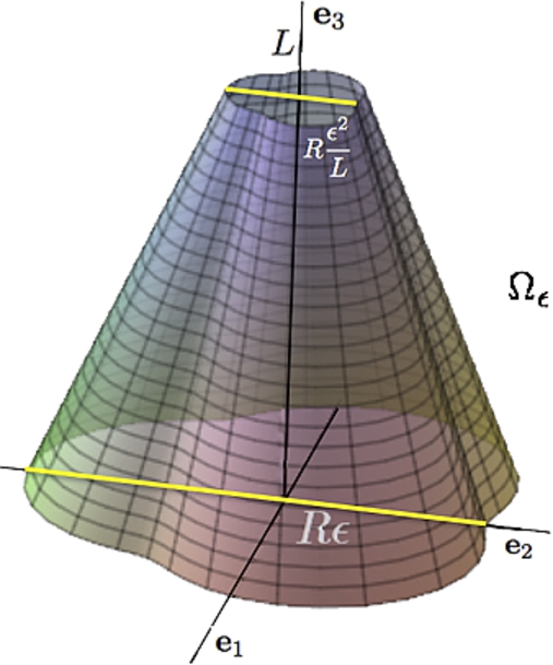
Notice that the center line of the straight rod is the coordinate axis . Moreover, the thickness of the thin rod depends on , it is given by the function . Observe that the diameter of the lower boundary is order ϵ while the diameter of the upper boundary is order . (See Fig. 1.)
Straight rod . (Colors are visible in the online version of the article; https://dx-doi-org.web.bisu.edu.cn/10.3233/ASY-151313.)
Now, we define an elementary displacement associated to a displacement of the rod.
The elementary displacement , associated to , is given by:
where for a.e.
The first component of is the displacement of the center line. The second component represents the rotation of the cross-section. Under the action of an elementary displacement the cross-section is translated by and it is rotated around the vector with an angle , where is the Euclidean norm in . Observe that, the torsion of the rod is given by the displacement .
Any displacement u of the rod can be decomposed as
The displacement is the warping.
Next theorem gives estimates of the components of the elementary displacement and of the warping in terms of ϵ, and of the strain energy of the displacement u. Notice that if u belongs to the functions and belong to .
Letandthe decomposition given by (2.2) and (2.3). Then the following estimates hold:The constants are independent of ϵ and L.
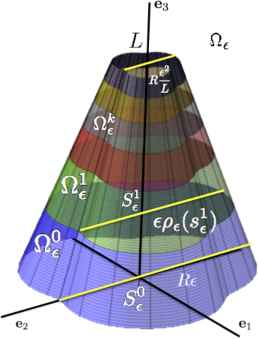
To prove the above estimates we are going to introduce a partition of the rod in several small portions, see Fig. 2, where every of these small rods are star-shaped with respect to suitable balls which verify that the ratio between their radius and the diameters of the portions remains uniformly bounded. Then we use the approximation of the displacement u by a rigid body displacement in each portion (see Theorem 2.3 in [19]).
Construction of the partition.
We start by considering the first portion of the rod
First, notice that has a diameter less than and all the cross-sections of are star-shaped with respect to a disc of radius . Therefore, by a simple geometrical argument, it is easy to check that this portion is star-shaped with respect to a ball of radius .
We consider now a partition of the interval defined as
Hence, the points of the partition are the elements of an arithmetico-geometric sequence
It makes sense to define as the largest integer such that .
The ()-portion of the rod is defined as
and
Therefore, we obtain
Rigid body approximation of u in the portions.
Partition of straight rod . (Colors are visible in the online version of the article; https://dx-doi-org.web.bisu.edu.cn/10.3233/ASY-151313.)
Since () is obtained by transforming by a dilation of ratio we can conclude that () is star-shaped with respect to a ball of radius and its diameter is less than . Moreover, the last portion is star-shaped with respect to a ball of radius and its diameter is less than .
From Theorem 2.3 in [19] there exists a rigid body displacement () such that
The constants depend only on the reference cross-section ω and on the ratio between the diameter of the portion and the radius of the ball inside (see Theorem 2.3 in [19])
Observe that for the last portion the ratio is less than .
Recall that the rigid body displacements are of the form
Now, we are going to prove ()1
If we have to replace by L.
The constants do not depend on k and ϵ.
The proof is similar for both inequalities, we will show only the first one. Taking the mean value of over the cross-sections of the portion and by the definition of the elementary displacement and (2.1) we have
Then using (2.5)1 and taking into account (2.6) we obtain the expected estimate
where the constant does not depend on ϵ and k.
Consequently, from (2.7) and (2.8), taking into account the definition of the elementary displacement and we have
Thus, we can replace by in (2.5)1
Moreover, since for , we get
Adding all these inequalities leads to the first estimate involving the warping
First of all, we compute the derivative of with respect to . Since the diameter of the cross-section depends on we rewrite performing a change of variables
where . The derivative is given by
Undoing the change of variables we get
From (2.5) we have
Moreover, from (2.8) we may replace by
Adding all these inequalities we obtain
Taking into account (2.1) we have for a.e.
Using (2.10) leads to ()2
If we have to replace by L.
Hence, since for we obtain
Adding all these inequalities we get the desired estimate
First of all, we introduce the function:
To calculate the derivative with respect to we perform a change of variables which allows us to write the function V as follows:
Then deriving with respect to gives (for a.e. )
Undoing the change of variables we have (for a.e. )
In view of (2.1) we can write (for a.e. )
Using (2.9) and (2.11) leads to ()3
If we have to replace by L.
Thus, since for and adding all these inequalities we have
Since we get the required estimate
Fourth estimate.
Observe that
From these expressions and taking into account (2.10), (2.12) and (2.13) we can conclude
which ends the proof. □
Estimates for the clamped rod at the bottom
From now on, we will assume that the rod is clamped at the bottom, . Then the space of admissible displacements of the rod is
Observe that the elementary displacement associated to any is equal to zero in the fixed part of the rod, .
Using estimates (2.4) and the boundary condition we deduce estimates on , and .
Assuming the rod clamped at the bottom, then we haveThe constants are independent of ϵ and L.
We begin with the proof of the first estimate in (3.1). Since by integration by parts we have
Then taking into account the facts that () and we get
Hence, by the Cauchy’s inequality it follows that:
Finally, the above inequalities together with the third estimate in (2.4) allow us to obtain the required estimate
The constant is independent of ϵ and L.
The second estimate follows from (2.4)2 and (3.2):
From the second estimate in (2.4) we obtain a better estimate for
Finally, the estimates for follow by a similar computation to . We first prove
then due to (3.1)2–(3.1)3 we get (3.1)4–(3.1)5. □
In view of the definition of the elementary displacement (2.2) we can write explicitly the components of the displacement, the gradient and the symmetric gradient of the displacement
Notice that, due to the definition of , and (2.1) we know that the warping satisfies
The previous Lemma 3.1 allows us to establish the Korn’s inequality for any displacement .
Assuming the rod clamped at the bottom boundary, then we haveThe constant does not depend on ϵ and L.
Recall that any displacement can be written as . Then we get
Using (3.7), (2.4) and (3.1) one has the following estimate:
Recall that . Consequently, we obtain the first estimate in (3.9).
In view of (3.5) and taking into account estimates (2.4) and (3.1) we obtain
which ends the proof. □
Rescaling of the rod
In this paragraph we define an operator which changes the scale. It allows us to transform the rod into a domain independent of ϵ.
Set , the reference beam. We rescale using the following operator:
defined for any function ϕ measurable on .
Observe that, if then and we have
Therefore, taking into account this above relation, we get the estimate for the rescaled warping
In order to obtain the estimates for the derivatives of the warping observe that for any
We recall that , then from (2.4) and (3.10) we get
In the same way, all the estimates in the previous sections over can be easily transposed over Ω.
Asymptotic behavior of a sequence of displacements
Now we consider a sequence of admissible displacements , where , satisfying
the constant does not depend on ϵ.
We are interested to describe the behaviour of the sequence as . In the following proposition we introduce the weak limits of the fields of the displacement’s decomposition in the rod. We denote by , , the strong limit in of . Observe that
First of all, we introduce certain weighted Lebesgue and Sobolev spaces defined in the interval .
, , consists of locally summable functions equipped with the following norm:
Observe that, there exists a linear homeomorphism of onto
Then endowed with the norm above is a Banach space.
Observe that if is a sequence of functions belonging to and satisfying weakly in then weakly in . Conversely, if is a sequence of functions such that is uniformly bounded in and satisfies weakly in then weakly in . Here k belongs to .
We define the space as follows:
endowed with the following norm:
We use this norm since as in the proof of Lemma 3.1 we can easily obtain
Since , , is locally integrable we can conclude that is a Banach space, see [20].
Analogously, and are the Banach spaces which contain the functions such that
We define their norms to be
We can easily prove that
then (4.2) yields for any .
Similarly we define some weighted spaces in the fixed domain Ω
They are Banach spaces endowed with their respective norms
Letbe a sequence of displacements such thatandwhere the constant C is independent of ϵ. Then for a subsequence, still denoted by,
there exist,andsuch that,
there exist,andsuch thatMoreover, we have the following relations between the limit fields:
First we get the weak limits, up to a subsequence still denoted by ϵ, of the different fields. Then we derive a few relations between some of them.
The convergences.
Taking into account (4.1)–(4.2) and (3.1)2–(3.1)3 we have
Then we obtain the following convergences:
According to (4.1) we get
Due to estimates (2.4)3 and (4.3) we obtain
Again due to (4.1) we have
In view of estimate (2.4)2 we get
Thanks to the estimates (3.11) and (3.13) the sequence is bounded in . Then we obtain
From property (3.10) of the rescaling operator and the estimate (3.9)2 we have
Moreover, taking into account the derivation rule (3.12) and the estimate (3.9)1 we have
Therefore, from (4.16), (4.17) and (4.18) we get
In the same way, from (3.9)1, (3.9)3 and (3.12) we obtain
Hence, we get
From the definition of the elementary displacement we have
Hence, in view of (3.1)1, (3.11), the property (3.10) of the rescaling operator and the assumption (4.4) we obtain the following estimate:
Now using the rule of the derivation (3.12) and (3.10) we have for
Consequently, from the two above estimates and (4.22) we get the last weak convergence
Relations between the limit fields.
Now we are going to establish the relations between the weak limits. First consider (2.4)2 which implies
as ϵ tends to 0. Then (4.5) and (4.7) give
It follows that for .
Now, from (3.5) we can write
In view of (4.5), (4.7), (4.10) and (4.11) by passing to the limit in (4.24) we obtain
Repeating the above arguments for we conclude that
Notice that does not depend on the variables for .
From (3.5) we have for a.e.
Now, using (4.6), (4.7), (4.10) and (4.12) we pass to the limit in the equality above and we get
Observe that, due to (4.23), (4.25) can be written as
Now we turn to the identification of . In view of (3.5) we have
From (4.7), (4.10), (4.13) by passing to the limit in (4.27) we obtain
Proceeding as above for we get
Finally we obtain the expression for . From (3.5) we have
Convergences (4.7), (4.10), (4.13) allow to pass to the limit and we get
Equivalently, from (4.23) we have
It is worth to note that the limit displacement field is a kind of Bernoulli–Navier displacement.
Also observe that the limit warping verifies the following conditions:
To conclude this section, we give the asymptotic behavior of the gradient and the symmetric gradient. We define the field by setting
Since and are independent of and we have
Then in view of (4.5), (4.6), (4.7) and (4.14) we obtain
Determination of the matrix T.
From (3.12) we have
Then in view of (3.8) and using convergence (4.10) we obtain
Applying the rescaling operator to (3.8) we get
Convergences (4.7), (4.8), (4.10) and (4.31) allow us to pass to the limit and we obtain
Similar calculations which are not repeated here allows us to get
To identify observe that from (3.8) we have
Convergences (4.6), (4.7), (4.10) and (4.31) allow us to pass to the limit and we obtain
According to (4.14), can be expressed as
Position of the elastic problem
We consider the standard linear isotropic equations of elasticity in . The displacement field in is denoted by
The linearized deformation field in is defined by
The Cauchy stress tensor in is linked to through the standard Hooke’s law
where λ and μ denotes the Lame’s coefficients of the elastic material and if and if . The equation of equilibrium in is
where denotes the applied force.
We assume that the rod is clamped at the bottom,
and at the boundary it is free
where denotes the exterior unit normal to .
Taking into account that the space of admissible displacements of the rod is
the variational formulation of (5.1) is
For any , the total elastic energy is denoted by
Observe that there exists a constant which depends only on λ and μ such that for any we have
Taking in (5.2) leads to the usual energy relation
Assumption on the forces
In view of the energy relation (5.4) and the estimates of the previous sections we assume throughout the paper
where and they satisfy
the constant does not depend on ϵ. Moreover, we assume the following weak convergences:
As a consequence, from (5.4) and the relations (3.6) we get an estimate of the total elastic energy
Due to (3.1)1, (3.1)4, (3.1)5 and (5.3)–(5.6) we have
That leads to
Hence
Observe that the assumptions on the applied forces were assumed in order to obtain the appropriate estimate on the energy naturally.
The limit problems
In this section we obtain the equations satisfied by the limit fields , and . To do this, we assume that the forces are given by (5.5) and satisfy (5.6)–(5.7). First, we apply the rescaling operator to the original variational formulation of the problem (5.2)
We will pass to the limit in (6.1) as ϵ tends to zero. In order to accomplish this we need specific choices of the test function v. We begin studying the behavior of the limit of the residual displacement .
Equations for
Let ϕ be in and φ be in such that , we define the test function by
Then we have
Hence, using the properties of the rescaling operator we get the following strong convergences in :
Moreover, , and are independent of ϵ, since
Now, we take as test function in (6.1), we have
Then we pass to the limit. As far as the right-hand side of (6.1) is concerned, taking into account the assumptions (5.5)–(5.6) and (5.7) we have
Hence, dividing by ϵ the right-hand side of (6.1) and passing to the limit gives
On the other hand, using the convergences (6.3), (6.4) and (4.29) we obtain the convergence of the left-hand side (divided by ϵ) when ϵ goes to 0
where ϕ be in and φ be in such that . Due to the convergence (6.5), the above limit is equal to zero. Since φ is arbitrary, we can localized with respect to ; that gives
Determination of
First, we choose . In view of (6.7) we have
Then the field satisfies
Now, we introduce the function χ as the unique solution of the following torsion problem:
Taking χ as test function in (6.9) gives
By contradiction, we easily prove . We set
The above constant which depends on the geometry of the reference cross section ω, is the St. Venant torsional stiffness.
Since verifies (6.8) and also for a.e. in , we get
which in turn gives
Determination of ,
Now taking in (6.7) yields
for any (). Then the variational problem (6.12) corresponds to a classical 2D elastic problem for . Taking into account the relations (4.28), the above variational problem admits a unique solution. Then we obtain
where is the Poisson coefficient of the material.
As a consequence we get
Equations for , and
Now we consider the functions , and in such that . We construct a test field as follows:
Then we get
Applying the rescaling operator to the previous expressions gives
In order to obtain the limit problem as ϵ tends to 0, we consider in (6.1), it leads to
We divide the above equality by . Then using the convergence (4.29) and the definition of the test function we can pass to the limit in the left-hand side to obtain
Moreover, taking into account (6.11) and (6.16), the above limit is equal to
where is the Young’s modulus of the elastic material.
On the other hand, in view of the assumptions (5.5), (5.7) and the definition of the test field we obtain the following limit for the right-hand side:
Hence, by (6.18) and (6.19) the limit equation of (6.17) is given by
for any such that and for such that . We simplify (6.20)
First we choose in (6.21). Taking into account the boundary condition , the function is the unique solution of
where K is given by (6.10).
In (6.21) we take . Since and are arbitrary in such that , that gives the bending problems satisfied by and
Recall that in order to obtain (6.22)–(6.23), we have used the fact that .
Equation for
In this step we derive the equation satisfied by . In order to get this, in (6.1) we consider as test field in such that with . Due to the assumptions (5.5), (5.7), the definition of the test field v and taking into account (2.1) the limit of (6.1) divided by ϵ gives
Hence, since φ is any function in such that and we can conclude that verifies the following compression–traction equation for elastic rods:
Convergence of the total elastic energy
In the above subsections all the limit problems admit a unique solution. As a consequence the whole sequences , , and converge weakly to their limit.
In this subsection we prove that the rescaled energy converges to the elastic limit energy as ϵ tends to zero and that some weak convergences are in fact strong convergences.
Under the assumptions (5.5), (5.6) and (5.7) on the applied forces, we obtain the following convergence for the total elastic energywhere T is the limit of the symmetric gradient defined in (4.29).
Taking in (5.2), dividing by , then using the properties of and by standard weak lower-semi-continuity, we obtain
We have
The last term in the above equality is equal to
Then (3.11), (4.7), (4.11), (4.12), (4.15) and (5.7) lead to
Besides, since T is a symmetric matrix we know that it verifies the following algebraic identity
Then, in view of (2.1), (4.32), (6.11), (6.16) and (6.9) we have
We recall that
Finally we obtain
which gives us the convergence of the rescaled energy to the total energy of the problems (6.23), (6.24) and (6.22) as ϵ goes to zero. □
Now we can deduce the strong convergences of the fields of the displacement decomposition using the strong convergence of the energy. In view of the weak convergence of the symmetric gradient (4.29), the strict convexity of the elastic energy implies that the convergence of the symmetric gradient is strong
As a consequence we get
Moreover, using for , and taking into account convergence (4.30) we may deduce from (6.30) that
as ϵ tends to zero. Then, in view of the weak convergences (4.6) and (4.7), (6.31) implies that
Moreover, from (4.8) and (6.33) we have
Hence, due to the decomposition (3.5) and the previous strong convergences we deduce
We also have
We recall that the warping functions satisfy (4.28). Then from the 2D Korn inequality we derive
That leads to
Conclusion
In this last section we summarize the results obtained in the previous sections.
Letbe the solution of the elasticity problem (5.2). Under the assumptions (5.5)–(5.7) on the applied forces, the sequencesatisfies the following convergenceswhereis the solution of the bending problem (6.23) andis the weak solution of the stretching problem (6.24). Moreover, we havewherewithis the solution of the torsion problem (6.9) andthe weak solution of (6.22).
Footnotes
Acknowledgements
Part of this work was done while the second author was visiting the Laboratoire J.-L. Lions in Paris. This author would like to acknowledge the warm hospitality of all the members of this institution. The second author was partially supported by Grant MTM2012-31298, MINECO, Spain and Grupo de Investigación CADEDIF, UCM and by a FPU fellowship (AP2010-0786) from the Government of Spain.
References
1.
J.M.Arrieta and M.Villanueva-Pesqueira, Locally periodic thin domains with varying period, Comptes Rendus Mathématique352(5) (2014), 397–403.
2.
D.Blanchard, A.Gaudiello and G.Griso, Junction of a periodic family of elastic rods with a 3d plate. Part I, J. Math. Pures Appl. (1)88 (2007), 1–33.
3.
D.Blanchard, A.Gaudiello and G.Griso, Junction of a periodic family of elastic rods with a thin plate. Part II, J. Math. Pures Appl. (2)88 (2007), 149–190.
4.
D.Blanchard and G.Griso, Microscopic effects in the homogenization of the junction of rods and a thin plate, Asymp. Anal.56(1) (2008), 1–36.
5.
P.G.Ciarlet, Mathematical Elasticity, Volume I, Three Dimensional Elasticity, North-Holland, 1988.
6.
P.G.Ciarlet, Mathematical Elasticity, Volume II, Theory of Plates, North-Holland, 1997.
7.
P.G.Ciarlet, Mathematical Elasticity, Volume III, Theory of Shells, North-Holland, 2000.
8.
D.Cioranescu, A.Damlamian, P.Donato, G.Griso and R.Zaki, The periodic unfolding method in domains with holes, SIAM J. Math. Anal.44(2) (2012), 718–760.
9.
D.Cioranescu, A.Damlamian and G.Griso, Periodic unfolding and homogenization, C. R. Acad. Sci. Paris Sér. I335 (2002), 99–104.
10.
D.Cioranescu, A.Damlamian and G.Griso, The periodic unfolding method in homogenization, SIAM J. Math. Anal.40(4) (2008), 1585–1620.
11.
A.Damlamian, An elementary introduction to periodic unfolding. Multi scale problems and asymptotic analysis, GAKUTO Internat. Ser. Math. Sci. Appl.24 (2006), 119–136.
12.
A.Damlamian and K.Pettersson, Homogenization of oscillating boundaries, Discrete Contin. Dyn. Syst.23(1-2) (2009), 197–219.
13.
G.Griso, Asymptotic behavior of structures made of plates, C. R. Acad. Sci. Paris Sér. I336 (2003), 101–106.
14.
G.Griso, Comportement asymptotique d’une grue, C. R. Acad. Sci. Paris Sér. I338 (2004), 261–266.
15.
G.Griso, Asymptotic behavior of curved rods by the unfolding method, Mod. Meth. Appl. Math.27(4) (2004), 2081–2110.
16.
G.Griso, Décomposition des déplacements d’une poutre. Simplification d’un problème d’élasticité, C. R. Acad. Sci. Paris Mécanique333(6) (2005), 475–480.
17.
G.Griso, Asymptotic behavior of structures made of plates, Analysis Appl.3(4) (2005), 325–356.
18.
G.Griso, Obtention d’équations de plaques par la méthode d’éclatement appliquée aux équations tridimensionnelles, C. R. Acad. Sci. Paris Sér. I343 (2006), 361–366.
19.
G.Griso, Decomposition of displacements of thin structures, J. Math. Pures Appl.89 (2008), 199–233.
20.
A.Kufner and B.Opic, How to define reasonably weighted Sobolev spaces, Commentationes Mathematicae Universitatis Carolinae25(3) (1984), 537–554.
21.
J.Sanchez-Hubert and E.Sanchez-Palencia, Statics of curved rods on account of torsion and flexion, European Journal of Mechanics – A/Solids18(3) (1999), 365–390.
22.
L.Trabucho and J.M.Viaño, Mathematical modelling of rods, in: Finite Element Methods (Part 2), Numerical Methods for Solids (Part 2), Handbook of Numerical Analysis, Vol. 4, North-Holland, Amsterdam, 1996, pp. 487–974.