Asymptotic expansion for the solution to a boundary-value problem in a thin cascade domain with a local joint

Abstract

A nonuniform Neumann boundary-value problem is considered for the Poisson equation in a thin domain $Ω_{ε}$ coinciding with two thin rectangles connected through a joint of diameter $O (ε)$ . A rigorous procedure is developed to construct the complete asymptotic expansion for the solution as the small parameter $ε \to 0$ . Energetic and uniform pointwise estimates for the difference between the solution of the starting problem ( $ε > 0$ ) and the solution of the corresponding limit problem ( $ε = 0$ ) are proved, from which the influence of the geometric irregularity of the joint is observed.

Keywords

asymptotic expansion asymptotic estimate thin domain with a local geometrical irregularity

1. Introduction

In recent years, the development of modern technologies of production of porous, composite, and other microinhomogeneous materials and biological structures has stimulated a significant interest in the investigation of boundary-value problems in thin domains (one of linear sizes of such a domain is substantially smaller than the others) with more complex structures: periodic grids and frames [1,6,8,29–31], junctions of thin domains [5,10,11,13,18,20–23,25–28], thick junctions of thin domains [2,3,14,16], thick multi-level, cascade and fractal junctions [7,9,15].

Such constructions of thin domains are successfully used in nanotechnologies, microtechnique, modern engineering constructions, as well as many physical and biological systems. Special interest of researchers is focused on various effects observed in vicinities of local irregularities of the geometry (widening or narrowing) of channels (e.g., adhesion to the walls, welds, and stenosis). Also the study of influence of local geometrical irregularities is very important in engineering, since such irregularities often directly affect the strength (stability, resistance, power, etc.) of constructions and devices. A fairly complete review on this topic has been presented in [10]. Results of recent theoretical, experimental and numerical studies of flows and wall-pressure fluctuations in channels with different types of narrowing are summarized in [4] and references therein.

It should be stressed that the error estimates and convergence rate are very important both for the justification of the adequacy of one- or two-dimensional models aimed at the description of actual three-dimensional thin bodies and for the study of boundary effects and effects of local (internal) inhomogeneities in applied problems. Particular importance for engineering practice is pointwise estimates for approximations, since large values of tearing stresses in small region at first involve local material damage and then the destruction of whole construction. Those estimates can be obtained and substantiated as a result of the development of new asymptotic methods that make it possible to build the leading terms of asymptotic approximations.

There are several rigorous approaches to study boundary-value problems in thin rod structures. Using the method of two-scale expansions, a complete asymptotic expansion in powers ε and μ for solutions of linear partial deferential equations in the simplest s-dimensional rectangular periodic carcass was constructed in [1] (here ε is the period of the carcass and ${(ε μ)}^{s - 1}$ is the area of the cross-section of beams).

The method of the partial asymptotic domain decomposition (MPADD), proposed in [24], was applied in the book [25] to the following problem in a finite thin rod structure $B_{ε}$ : $\begin{array}{rcl} Δ u = \{\begin{matrix} f^{e} ({\tilde{x}}_{1}) & in S_{0}, \\ 0 & in Π_{x_{0}} : = B_{ε} ∖ S_{0}, \end{matrix} \\ u |_{\partial_{1} B_{ε}} = 0, \frac{\partial u}{\partial n} |_{\partial_{2} B_{ε}} = 0, \end{array}$ where $S_{0}$ is the union of sections of the rod structure $B_{ε}$ , $Π_{x_{0}}$ is the connected component of $B_{ε} ∖ S_{0}$ containing the node $x_{0}$ . The main idea of this method to reduce the problem to a simplified form on $S_{0}$ , where the regular asymptotics of the solution is located, keeping the initial formulation on a small neighbourhood of the domain $Π_{x_{0}}$ , where the asymptotic behavior is singular. Then these two models are coupled by some special interface conditions that are derived from some projection procedure. For this, the author proposed a method of redistribution of constants to have the boundary-layer solutions exponentially decaying at infinity. As a result, for the leading term of the asymptotic expansion the following estimate was obtained: $\begin{matrix} (1) & \frac{‖ u - v ‖_{L^{2} (B_{ε})}}{\sqrt{meas (B_{ε})}} = O (\sqrt{ε}) . \end{matrix}$ Then this method was developed to construct the complete asymptotic expansions both for the solution of the wave equation on a thin rod structure [26] and for the solution of the following non-steady Navier–Stokes equations in a thin tube structure $B_{ε}$ (see [27,28]): $\begin{array}{l} v_{t} - ν Δ v + (v \cdot \nabla) v + \nabla p = 0, div v = 0, \\ v |_{⋃_{j = N_{1} + 1}^{N} σ_{ε}^{j}} = g (x, t), v |_{\partial B_{ε} ∖ (⋃_{j = N_{1} + 1}^{N} σ_{ε}^{j})} = 0, v (x, 0) = 0, \end{array}$ where ${σ_{ε}^{j}}_{j = N_{1} + 1}^{N}$ are bases of the cylinders ${Π_{ε}^{(e_{j})}}_{j = N_{1} + 1}^{N}$ associated to the vertices $O_{N_{1} + 1}, \dots, O_{N}$ of $B_{ε}$ . We see that this method (MPADD) was applied to boundary-value problems in thin rod structures in the case of the uniform boundary conditions on the lateral surfaces of thin rods (cylinders) and if the right-hand sides depend only on the longitudinal variable in the direction of the corresponding rod and they are constant in some neighbourhoods of the nodes and vertices.

In papers [21,22] the equations of anisotropic elasticity on junctions of thin beams ( $2 D$ and $3 D$ cases) were considered. Only the leading terms of the elastic-field asymptotics are constructed and estimates for asymptotic remainders were derived under the following assumptions:

the first terms of the volume force f and surface load g on the rods satisfy special orthogonality conditions (see (3.5)₁ and (3.6) in [22]) and the second term of the volume force f has an identified form and depends only on the longitudinal variable;

similar orthogonality conditions for the right-hand sides on the knots are satisfied (see (3.41)) and the second term is a piecewise constant vector-function (see (3.42)).

Thanks to these assumptions the displacement field at each knot can be approximated by the rigid displacement. As a result, the approximation contains no terms of boundary-layer terms, i.e. the asymptotic expansion is not complete a priori [22, Remark 3.1].

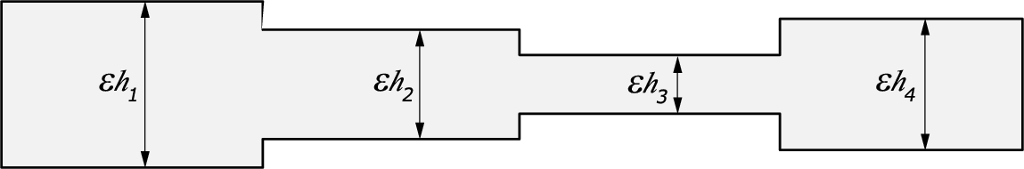
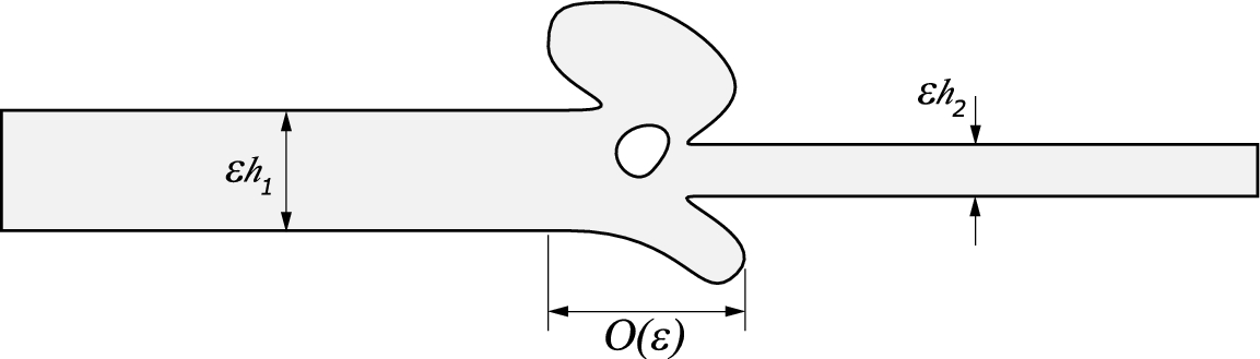
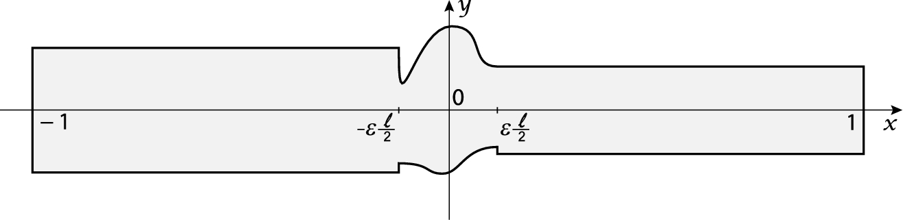
In [13] we proved the error estimates and constructed the asymptotic expansion for the solution of a boundary-value problem in a thin cascade domain without joints (see Fig. 1). The present paper is devoted to further development of the asymptotic method proposed in [13]. Namely, we consider a nonuniform Neumann boundary-value problem for the Poisson equation with the right-hand side that depends both on longitudinal and transversal variables in a thin cascade domain that consists of two thin rectangles of different thicknesses and local geometric irregularity (the joint) between them (this can be either a local widening (see Fig. 2) or local narrowing (see Fig. 3)).

Fig. 1.

Thin cascade domain without local joints.

Fig. 2.

Thin cascade domain with a local widening.

Fig. 3.

Thin cascade domain with a local narrowing.

A principal new feature of this paper in comparison with the papers mentioned above is the construction and justification of the complete asymptotic expansion for the solution and the proof both energetic and pointwise uniform estimates for the difference between the solution of the starting problem ( $ε > 0$ ) and the solution of the corresponding limit problem ( $ε = 0$ ) without any orthogonality condition for the right-hand side $f (x, \frac{y}{ε})$ in the Poisson equation and for the right-hand sides in the Neumann boundary conditions. To construct the asymptotic expansion in the whole domain we use the method of matching of asymptotic expansions (see [12]) with special cut-off functions. In this approach the inner boundary-layer solutions take into account the behaviour of the regular part of the asymptotics and the right-hand sides in a neighbourhood of the joint. In addition, these boundary-layer solutions have polynomial grow at the infinity. Matching the regular part of the asymptotics with the singular one, we derive the corresponding transmission conditions. As a result, it became possible to identify more precisely the impact of the geometric irregularity and material characteristics of the joint on some properties of the whole structure. In addition to the pointwise uniform estimates, we obtain also the energetic estimate (see Corollary 4.1) $\begin{matrix} (2) & \frac{‖ u - v ‖_{H^{1} (Ω_{ε})}}{\sqrt{meas (Ω_{ε})}} = O (\sqrt{ε}) \end{matrix}$ in the Sobolev space $H^{1} (Ω_{ε})$ (instead of $L^{2}$ -space in (1)). Also our results confirm and complement some of conclusions of [10], on the other hand they show that the main assumptions made in this article are not correct. A more informative discussion is given in the last section of the present paper.

As we will see, there is no essential difference between the construction of the asymptotic expansion in 2- or 3-dimensional domains. Therefore, to simplify calculations, we consider the two-dimensional case. The paper is organized as follows. In Section 3, we construct the formal asymptotic expansion for the solution to the problem (3). To perform this we generalize the asymptotic method for boundary-value problems in thin domains with constant thickness proposed in the monograph [19]. In particular, we introduced a special inner asymptotic expansion in a neighborhood of the joint, determine its coefficients and study some their properties as solutions to corresponding boundary-value problems in an unbounded domain. Thus, the asymptotics for the solution consists of three parts: the regular part, the boundary parts near the extreme vertical sides and the inner part in a neighborhood of the joint. In Section 4, we justify the asymptotics (Theorem 4.1) and prove asymptotic estimates for the leading terms of the asymptotics (Corollary 4.1). In Section 5 we analyze results obtained in this paper and discuss possible generalizations.

2. Statement of the problem

The model thin cascade domain $Ω_{ε}$ consists of two thin rectangles $\begin{matrix} Ω_{ε}^{(1)} = ((- 1, - ε \frac{l}{2}) \times Υ_{ε}^{(1)}) and Ω_{ε}^{(2)} = ((ε \frac{l}{2}, 1) \times Υ_{ε}^{(2)}) \end{matrix}$ that are joined through $Ω_{ε}^{(0)}$ (referred in the sequel “joint”). Here $Υ_{ε}^{(i)} = (- ε \frac{h_{i}}{2}, ε \frac{h_{i}}{2})$ , $i = 1, 2$ ; ε is a small parameter; l, $h_{1}$ and $h_{2}$ are fixed positive constants.

The joint $Ω_{ε}^{(0)}$ are formed by the homothetic transformation with the coefficient ε from a domain $Ξ^{(0)}$ , i.e., $Ω_{ε}^{(0)} = ε Ξ^{(0)}$ . In addition, we assume that $\begin{matrix} Ω_{ε}^{(0)} \cap {(x, y) : | y | ⩽ ε max {h_{1}, h_{2}}} \subset {(x, y) : | x | ⩽ (- ε \frac{l}{2}, ε \frac{l}{2})} \end{matrix}$ and the interior of the union $\begin{matrix} \overline{Ω_{ε}^{(1)}} \cup \overline{Ω_{ε}^{(0)}} \cup \overline{Ω_{ε}^{(2)}} \end{matrix}$ is a domain with the Lipschitz boundary, which we denote by $Ω_{ε}$ (see e.g. Fig. 4).

Fig. 4.

The model thin cascade domain $Ω_{ε}$ with a local geometric irregularity.

Remark 2.1.

As an example of the joint we can consider the following domain: $\begin{matrix} Ω_{ε}^{(0)} = ε Ξ^{(0)} = {(x, y) : - ε h_{0}^{-} (\frac{x}{ε}) < y < ε h_{0}^{+} (\frac{x}{ε}), y \in (- ε \frac{l}{2}, ε \frac{l}{2})}, \end{matrix}$ where $Ξ^{(0)} = {(ξ, η) : - h_{0}^{-} (ξ) < η < h_{0}^{+} (ξ), ξ \in (- \frac{l}{2}, \frac{l}{2})}$ , the functions $h_{0}^{-}$ and $h_{0}^{+}$ belong to the space $C^{1} ([- \frac{l}{2}, \frac{l}{2}])$ , take positive values on the segment $[- \frac{l}{2}, \frac{l}{2}]$ and $h_{0}^{\pm} (- \frac{l}{2}) ⩽ h_{1}$ , $h_{0}^{\pm} (\frac{l}{2}) ⩽ h_{2}$ . With the help of functions $h_{0}^{-}$ and $h_{0}^{+}$ it is possible to describe both a local narrowing and a local widening.

In the domain $Ω_{ε}$ , we consider the following mixed boundary-value problem: $\begin{matrix} (3) & \{\begin{matrix} - Δ u_{ε} (x, y) = f (x, \frac{y}{ε}), & (x, y) \in Ω_{ε}, \\ - \partial_{ν} u_{ε} (x, y) |_{y = \pm ε \frac{h_{i}}{2}} = ε φ_{\pm}^{(i)} (x), & x \in I_{ε}^{(i)}, i = 1, 2, \\ u_{ε} (- 1, y) = 0, & y \in Υ_{ε}^{(1)}, \\ u_{ε} (1, y) = 0, & y \in Υ_{ε}^{(2)}, \\ \partial_{ν} u_{ε} (x, y) = 0, & (x, y) \in Γ_{ε}, \end{matrix} \end{matrix}$ where $I_{ε}^{(1)} = (- 1, - ε \frac{l}{2})$ , $I_{ε}^{(2)} = (ε \frac{l}{2}, 1)$ , $\partial_{ν}$ is the outward normal derivative, and the boundary of the joint is described by the formula $\begin{matrix} Γ_{ε} = \partial Ω_{ε} ∖ (⋃_{i = 1}^{2} ((I_{ε}^{(i)} \times {\pm ε \frac{h_{i}}{2}}) \cup ({{(- 1)}^{i}} \times Υ_{ε}^{(i)}))) . \end{matrix}$

Assume that the given functions f and ${φ_{\pm}^{(i)}}$ are smooth in the corresponding domains of definition.

It follows from the theory of linear boundary-value problems that, for any fixed value of ε, problem (3) possesses a unique weak solution $u_{ε}$ from the Sobolev space $H^{1} (Ω_{ε})$ such that its traces on the vertical end sides of the domain $Ω_{ε}$ are equal to zero, i.e., $u_{ε} |_{x = \pm 1} = 0$ , and the solution satisfies the integral identity $\begin{matrix} (4) & \int_{Ω_{ε}} \nabla u_{ε} \cdot \nabla ψ d x d y = \int_{Ω_{ε}} f ψ d x d y \mp ε \sum_{i = 1}^{2} \int_{I_{ε}^{(i)}} φ_{\pm}^{(i)} ψ d x \end{matrix}$ for any function $ψ \in H^{1} (Ω_{ε})$ such that $ψ |_{x = \pm 1} = 0$ .

Remark 2.2.

In the right-hand side of identity (4), we introduce the abridged notation $\begin{matrix} \mp ε \sum_{i = 1}^{2} \int_{I_{ε}^{(i)}} φ_{\pm}^{(i)} ψ d x : = - ε \sum_{i = 1}^{2} \int_{I_{ε}^{(i)}} φ_{+}^{(i)} ψ d x + ε \sum_{i = 1}^{2} \int_{I_{ε}^{(i)}} φ_{-}^{(i)} ψ d x \end{matrix}$ and use it in what follows.

The aim of the present paper is to construct and justify the asymptotic expansion of the solution $u_{ε}$ as $ε \to 0$ .

3. Formal asymptotic expansion

3.1. Regular part of the asymptotics

We seek the regular part of the asymptotics in the form $\begin{matrix} (5) & u_{\infty}^{(i)} : = \sum_{k = 2}^{+ \infty} ε^{k} (u_{k}^{(i)} (x, \frac{y}{ε}) + ε^{- 2} ω_{k}^{(i)} (x)), (x, y) \in Ω_{ε}^{(i)}, i = 1, 2 . \end{matrix}$ Formally substituting the series (5) into the differential equation and into the first boundary condition of problem (3), we obtain: $\begin{array}{rcl} - \sum_{k = 2}^{+ \infty} ε^{k} \partial_{x x}^{2} u_{k}^{(i)} (x, η) - \sum_{k = 2}^{+ \infty} ε^{k - 2} \partial_{η η}^{2} u_{k}^{(i)} (x, η) - \sum_{k = 2}^{+ \infty} ε^{k - 2} \frac{d^{2} ω_{k}^{(i)}}{d x^{2}} (x) \approx f (x, η), η = \frac{y}{ε}, \\ - \sum_{k = 2}^{+ \infty} ε^{k} \partial_{η} u_{k}^{(i)} (x, η) |_{η = \pm \frac{h_{i}}{2}} \approx ε^{2} φ_{\pm}^{(i)} (x), \end{array}$ where $\partial_{x} = \partial / \partial x$ , $\partial_{x x}^{2} = \partial^{2} / \partial x^{2}$ , $\partial_{η} = \partial / \partial η$ , $\partial_{η η}^{2} = \partial^{2} / \partial η^{2}$ .

Equating the coefficients of the same powers of ε, we deduce recurrent relations of the boundary-value problems for the determination of the expansion coefficients in (5). Let us consider the problem for $u_{2}^{(i)}$ : $\begin{matrix} (6) & \{\begin{matrix} - \partial_{η η}^{2} u_{2}^{(i)} (x, η) = f (x, η) + \frac{d^{2} ω_{2}^{(i)}}{d x^{2}} (x), & η \in Υ_{i}, \\ - \partial_{η} u_{2}^{(i)} (x, η) |_{η = \pm \frac{h_{i}}{2}} = φ_{\pm}^{(i)} (x), & x \in I_{ε}^{(i)}, \\ {⟨ u_{2}^{(i)} (x, \cdot) ⟩}_{Υ_{i}} = 0, & x \in I_{ε}^{(i)} . \end{matrix} \end{matrix}$ Here $Υ_{i} = (- \frac{h_{i}}{2}, \frac{h_{i}}{2})$ , ${⟨ u (x, \cdot) ⟩}_{Υ_{i}} : = \int_{Υ_{i}} u (x, η) d η$ , $i = 1, 2$ .

For each value of i, the problem (6) is the Neumann problem for the ordinary differential equation with respect to the variable $η \in Υ_{i}$ ; here, the variable x is regarded as a parameter. We now write the necessary and sufficient conditions for the solvability of problem (6) and obtain the following differential equation for the function $ω_{2}^{(i)}$ : $\begin{matrix} (7) & - h_{i} \frac{d^{2} ω_{2}^{(i)}}{d x^{2}} (x) = \int_{Υ_{i}} f (x, η) d η - φ_{+}^{(i)} (x) + φ_{-}^{(i)} (x), x \in I_{ε}^{(i)} (i = 1, 2) . \end{matrix}$ Let $ω_{2}^{(i)}$ be a solution of the differential equation (7) (boundary conditions for this differential equation will be determined later). Then the solution of problem (6) exist and the third relation in (6) supplies the uniqueness of solution.

For determination of the coefficients $u_{3}^{(i)}$ , $i = 1, 2$ , we obtain the following problems: $\begin{matrix} (8) & \{\begin{matrix} - \partial_{η η}^{2} u_{3}^{(i)} (x, η) = \frac{d^{2} ω_{3}^{(i)}}{d x^{2}} (x), & η \in Υ_{i}, \\ - \partial_{η} u_{3}^{(i)} (x, η) |_{η = \pm \frac{h_{i}}{2}} = 0, & x \in I_{ε}^{(i)} \\ {⟨ u_{3}^{(i)} (x, \cdot) ⟩}_{Υ_{i}} = 0, & x \in I_{ε}^{(i)} . \end{matrix} \end{matrix}$ Repeating the previous reasoning, we find $u_{3}^{(i)} \equiv 0$ and $\frac{d^{2} ω_{3}^{(i)}}{d x^{2}} (x) = 0$ , $x \in I_{ε}^{(i)}$ , $i = 1, 2$ .

Let us consider boundary-value problems for the functions $u_{k}^{(i)}$ , $k ⩾ 4$ , $i = 1, 2$ : $\begin{matrix} (9) & \{\begin{matrix} - \partial_{η η}^{2} u_{k}^{(i)} (x, η) = \frac{d^{2} ω_{k}^{(i)}}{d x^{2}} (x) + \partial_{x x}^{2} u_{k - 2}^{(i)} (x, η), & η \in Υ_{i}, \\ - \partial_{η} u_{k}^{(i)} (x, η) |_{η = \pm \frac{h_{i}}{2}} = 0, & x \in I_{ε}^{(i)}, \\ {⟨ u_{2}^{(i)} (x, \cdot) ⟩}_{Υ_{i}} = 0, & x \in I_{ε}^{(i)} . \end{matrix} \end{matrix}$ Assume that all coefficients $u_{2}^{(i)}, \dots, u_{k - 1}^{(i)}$ , $ω_{2}^{(i)}, \dots, ω_{k - 1}^{(i)}$ of the expansion (5) are determined. We find $u_{k}^{(i)}$ and $ω_{k}^{(i)}$ from problem (9). It follows from the solvability condition of problem (9) that $\begin{matrix} h_{i} \frac{d^{2} ω_{k}^{(i)}}{d x^{2}} (x) = - \int_{Υ_{i}} \partial_{x}^{2} u_{k - 2} (x, η) d η = - \partial_{x}^{2} (\int_{Υ_{i}} u_{k - 2}^{(i)} (x, η) d η) = 0, \end{matrix}$ i.e., $ω_{k}^{(i)}$ is a linear function solving the differential equation $\begin{matrix} (10) & \frac{d^{2} ω_{k}^{(i)}}{d x^{2}} (x) = 0, x \in I_{ε}^{(i)} . \end{matrix}$

Remark 3.1.
Boundary conditions for the differential equations (7) and (10) are unknown in advance. They will be determined in the process of construction of the asymptotics.

Thus, the solution of problem (9) is uniquely determined. Hence, the recursive procedure for the determination of the coefficients of series (5) is uniquely solvable. Remark 3.2.
By using the recursive procedure for the boundary-value problem (9), one can easily show that the functions $u_{2 p + 1}^{(i)}$ are identically equal to zero for odd $k = 2 p + 1$ , $p \in N$ .

3.2. Boundary asymptotics near the vertical sides of domain $Ω_{ε}$

In the previous section, we have considered the regular asymptotics taking into account the inhomogeneity of the right-hand side of the differential equation in (3) and the boundary conditions on the horizontal sides of the thin domain $Ω_{ε}$ . In what follows, we construct the boundary part of the asymptotics compensating the residuals of the regular part of the asymptotics at the left side of $Ω_{ε}^{(1)}$ and the right one of $Ω_{ε}^{(2)}$ .

At the left vertical part of the boundary of $Ω_{ε}^{(1)}$ , we seek the boundary asymptotics for the solution in the form $\begin{matrix} (11) & Π_{\infty}^{(1)} : = \sum_{k = 0}^{+ \infty} ε^{k} Π_{k}^{(1)} (\frac{1 + x}{ε}, \frac{y}{ε}) . \end{matrix}$ Substituting (11) into (3) and collecting coefficients with the same powers of ε, we obtain the following mixed boundary-value problems: $\begin{matrix} (12) & \{\begin{matrix} - Δ_{ξ η} Π_{k}^{(1)} (ξ, η) = 0, & (ξ, η) \in (0, + \infty) \times Υ_{1}, \\ - \partial_{η} Π_{k}^{(1)} (ξ, η) |_{η = \pm \frac{h_{1}}{2}} = 0, & ξ \in (0, + \infty), \\ Π_{k}^{(1)} (0, η) = Φ_{k}^{(1)} (η), & η \in Υ_{1}, \\ Π_{k}^{(1)} (ξ, η) \to 0, & ξ \to + \infty, η \in Υ_{1}, \end{matrix} \end{matrix}$ where $\begin{array}{rcl} ξ = \frac{1 + x}{ε}, η = \frac{y}{ε}, Φ_{k}^{(1)} = - ω_{k + 2}^{(1)} (- 1), k = 0, 1, \\ Φ_{k}^{(1)} (η) = - u_{k}^{(1)} (- 1, η) - ω_{k + 2}^{(1)} (- 1), k ⩾ 2 . \end{array}$

Using the method of separation of variables, we determine the solution $\begin{matrix} (13) & Π_{k}^{(1)} (ξ, η) = \sum_{p = 0}^{+ \infty} [a_{p}^{(1)} e^{- \frac{2 p π}{h_{1}} ξ} cos (\frac{2 p π}{h_{1}} η) + b_{p}^{(1)} e^{- \frac{(2 p + 1) π}{h_{1}} ξ} sin (\frac{(2 p + 1) π}{h_{1}} η)] \end{matrix}$ of problem (12) at a fixed index k, where $\begin{array}{rcl} a_{p}^{(1)} = \frac{2}{h_{1}} \int_{- \frac{h_{1}}{2}}^{\frac{h_{1}}{2}} Φ_{k}^{(1)} (η) cos (\frac{2 p π}{h_{1}} η) d η, b_{p}^{(1)} = \frac{2}{h_{1}} \int_{- \frac{h_{1}}{2}}^{\frac{h_{1}}{2}} Φ_{k}^{(1)} (η) sin (\frac{(2 p + 1) π}{h_{1}} η) d η, \\ a_{0}^{(1)} = \frac{1}{h_{1}} \int_{- \frac{h_{1}}{2}}^{\frac{h_{1}}{2}} Φ_{k}^{(1)} (η) d η = \frac{1}{h_{1}} \int_{- \frac{h_{1}}{2}}^{\frac{h_{1}}{2}} u_{k}^{(1)} (- 1, η) d η - ω_{k + 2}^{(1)} (- 1) = - ω_{k + 2}^{(1)} (- 1) . \end{array}$ It follows from the fourth condition in (12) that coefficient $a_{0}^{(1)}$ must be equal to 0. As a result, we arrive at the following boundary conditions for the functions ${ω_{k + 2}^{(1)}}$ : $\begin{matrix} (14) & ω_{k + 2}^{(1)} (- 1) = 0, k \in N_{0} . \end{matrix}$

At the left vertical part of the boundary of $Ω_{ε}^{(2)}$ , we seek the boundary asymptotics for the solution in the form $\begin{matrix} (15) & Π_{\infty}^{(2)} : = \sum_{k = 0}^{+ \infty} ε^{k} Π_{k}^{(2)} (\frac{1 - x}{ε}, \frac{y}{ε}) . \end{matrix}$ We obtain the following problems for the determination of the coefficients ${Π_{k}^{(2)}}_{k \in N_{0}}$ : $\begin{matrix} (16) & \{\begin{matrix} - Δ_{ξ^{*} η} Π_{k}^{(2)} (ξ^{*}, η) = 0, & (ξ^{*}, η) \in (0, + \infty) \times Υ_{2}, \\ - \partial_{η} Π_{k}^{(2)} (ξ^{*}, η) |_{η = \pm \frac{h_{2}}{2}} = 0, & ξ^{*} \in (0, + \infty), \\ Π_{k}^{(1)} (0, η) = Φ_{k}^{(2)} (η), & η \in Υ_{2}, \\ Π_{k}^{(1)} (ξ^{*}, η) \to 0, & ξ^{*} \to + \infty, η \in Υ_{2}, \end{matrix} \end{matrix}$ where $\begin{array}{rcl} ξ^{*} = \frac{1 - x}{ε}, η = \frac{y}{ε}, Φ_{k}^{(2)} = - ω_{k + 2}^{(2)} (1), k = 0, 1, \\ Φ_{k}^{(2)} (η) = - u_{k}^{(2)} (1, η) - ω_{k + 2}^{(2)} (1), k ⩾ 2 . \end{array}$

Similarly we find the following solution of problem (16) at a fixed index k: $\begin{matrix} (17) & Π_{k}^{(2)} (ξ^{*}, η) = \sum_{p = 0}^{+ \infty} [a_{p}^{(2)} e^{- \frac{2 p π}{h_{2}} ξ^{*}} cos (\frac{2 p π}{h_{2}} η) + b_{p}^{(2)} e^{- \frac{(2 p + 1) π}{h_{2}} ξ^{*}} sin (\frac{(2 p + 1) π}{h_{2}} η)], \end{matrix}$ where $\begin{array}{rcl} a_{p}^{(2)} = \frac{2}{h_{2}} \int_{- \frac{h_{2}}{2}}^{\frac{h_{2}}{2}} Φ_{k}^{(2)} (η) cos (\frac{2 p π}{h_{2}} η) d η, b_{p}^{(2)} = \frac{2}{h_{2}} \int_{- \frac{h_{2}}{2}}^{\frac{h_{2}}{2}} Φ_{k}^{(2)} (η) sin (\frac{(2 p + 1) π}{h_{2}} η) d η, \\ a_{0}^{(2)} = \frac{1}{h_{2}} \int_{- \frac{h_{2}}{2}}^{\frac{h_{2}}{2}} Φ_{k}^{(2)} (η) d η = \frac{1}{h_{2}} \int_{- \frac{h_{2}}{2}}^{\frac{h_{2}}{2}} u_{k}^{(2)} (1, η) d η - ω_{k + 2}^{(2)} (1) = - ω_{k + 2}^{(2)} (1) . \end{array}$ It follows from the fourth condition in (16) that the coefficient $a_{0}^{(2)}$ is equal to 0. This is possible if $\begin{matrix} (18) & ω_{k + 2}^{(2)} (1) = 0, k \in N_{0} . \end{matrix}$

Remark 3.3.
Since $u_{k}^{(i)} \equiv 0$ for $k = 2 p + 1$ , $p \in N$ , we conclude that $Φ_{k}^{(i)} = 0$ and, hence, $\begin{matrix} Π_{0}^{(i)} \equiv 0, Π_{2 p - 1}^{(i)} \equiv 0, p \in N, i = 1, 2 . \end{matrix}$ Moreover, from representation (13) and (17) it follows the following asymptotic relations $\begin{matrix} (19) & \begin{matrix} Π_{k}^{(1)} (ξ, η) = O (exp (- \frac{π}{h_{1}} ξ)) as ξ \to + \infty, \\ Π_{k}^{(2)} (ξ^{}, η) = O (exp (- \frac{π}{h_{2}} ξ^{})) as ξ^{*} \to + \infty . \end{matrix} \end{matrix}$

Equalities (14) and (18) specify the boundary conditions at points $- 1$ and 1 for all functions ${ω_{k}^{(1)}}$ and ${ω_{k}^{(2)}}$ , respectively.
3.3. Inner boundary part of the asymptotics

To obtain conditions for the functions ${ω_{k}^{(1)}}$ and ${ω_{k}^{(2)}}$ at the point 0, we introduce an additional internal asymptotics in a neighbourhood of the joint. For this we pass to the following variables $ξ = \frac{x}{ε}$ and $η = \frac{y}{ε}$ . Then forwarding the parameter ε to 0, we see that the domain $Ω_{ε}$ is transformed into the unbounded domain Ξ, which is the union of joint $Ξ^{(0)}$ and two half strips $Ξ^{(1)} = (- \infty, - \frac{l}{2}) \times Υ_{1}$ , $Ξ^{(2)} = (\frac{l}{2}, + \infty) \times Υ_{2}$ , i.e., Ξ is the interior of $\overline{Ξ^{(1)} \cup Ξ^{(0)} \cup Ξ^{(2)}}$ .

Let us introduce the following notation for parts of the boundary of the domain Ξ:

$\partial Ξ_{=}^{(i)}$ is the horizontal parts of the boundary $\partial Ξ^{(i)}$ , $i = 1, 2$ ,

$Γ = \partial Ξ ∖ (\partial Ξ_{=}^{(1)} \cup \partial Ξ_{=}^{(2)})$ .

We seek the inner expansion in the form $\begin{matrix} (20) & N_{\infty} = \sum_{k = 1}^{+ \infty} ε^{k} N_{k} (\frac{x}{ε}, \frac{y}{ε}) . \end{matrix}$ Substituting (20) into (3) and equating coefficients at the same powers of ε, we derive the following relations for ${N_{k}}$ : $\begin{matrix} (21) & \{\begin{matrix} - Δ_{ξ η} N_{k} (ξ, η) = F_{k} (ξ, η), & (ξ, η) \in Ξ, \\ \partial_{ν} N_{k} (ξ, η) = 0 & (ξ, η) \in Γ, \\ - \partial_{η} N_{k} (ξ, η) |_{η = \pm \frac{h_{i}}{2}} = B_{k_{\pm}}^{(i)} (ξ), & {(- 1)}^{i} ξ \in (\frac{l}{2}, + \infty), i = 1, 2, \\ N_{k} (ξ, η) \sim ω_{k + 2}^{(i)} (0) + Ψ_{k}^{(i)} (ξ, η), & {(- 1)}^{i} ξ \to + \infty, η \in Υ_{i}, i = 1, 2, \end{matrix} \end{matrix}$ where $\begin{array}{l} F_{0} \equiv F_{1} \equiv 0, F_{k} (ξ, η) = \frac{ξ^{k - 2}}{(k - 2)!} \frac{\partial^{k - 2} f}{\partial x^{k - 2}} (0, η), (ξ, η) \in Ξ, \\ B_{1_{\pm}}^{(i)} \equiv B_{1_{\pm}}^{(i)} \equiv 0, B_{k_{\pm}}^{(i)} (ξ) = \frac{ξ^{k - 2}}{(k - 2)!} \frac{d^{k - 2} φ_{\pm}^{(i)}}{d x^{k - 2}} (0), {(- 1)}^{i} ξ \in (\frac{l}{2}, + \infty), i = 1, 2, \\ (22) & \begin{matrix} Ψ_{0}^{(i)} \equiv 0, Ψ_{1}^{(i)} (ξ, η) = ξ \frac{d ω_{2}^{(i)}}{d x} (0), i = 1, 2, \\ Ψ_{k}^{(i)} (ξ, η) = ξ \frac{d ω_{k + 1}^{(i)}}{d x} (0) + \frac{ξ^{k}}{k!} \frac{d^{k} ω_{2}^{(i)}}{d x^{k}} (0) + \sum_{j = 0}^{k - 2} \frac{ξ^{j}}{j!} \frac{\partial^{j} u_{k - j}^{(i)}}{\partial x^{j}} (0, η), i = 1, 2, k ⩾ 2 . \end{matrix} \end{array}$

The right hand side and boundary conditions for problem (21) are obtained with the help of the Taylor decomposition of the functions f and $φ_{\pm}^{(i)}$ at the point $x = 0$ . The fourth condition in (21) appears by matching the regular and inner asymptotics in a neighborhood of the joint, namely the asymptotics of the terms ${N_{k}}$ as $ξ \to \pm \infty$ have to coincide with the corresponding asymptotics of terms of the regular expansions (5) as $x \to \pm 0$ , respectively. Expanding each term of the regular asymptotics in the Taylor series at the point $x = 0$ and collecting the coefficients of the same powers of ε with regard to (10), we get relations (22).

A solution of problem (21) is sought in the form $\begin{matrix} (23) & N_{k} (ξ, η) = Ψ_{k}^{(1)} (ξ, η) χ_{1} (ξ) + Ψ_{k}^{(2)} (ξ, η) χ_{2} (ξ) + {\tilde{N}}_{k} (ξ, η), \end{matrix}$ where $χ_{i} \in C^{\infty} (R_{+})$ , $0 ⩽ χ_{i} ⩽ 1$ and $\begin{matrix} χ_{i} (ξ) = \{\begin{matrix} 0, & if {(- 1)}^{i} ξ ⩽ 1 + \frac{l}{2}, \\ 1, & if {(- 1)}^{i} ξ ⩾ 2 + \frac{l}{2}, \end{matrix} i = 1, 2 . \end{matrix}$ Then ${\tilde{N}}_{k}$ has to be a solution of the following problem: $\begin{matrix} (24) & \{\begin{matrix} - Δ_{ξ η} {\tilde{N}}_{k} (ξ, η) = {\tilde{F}}_{k} (ξ, η), & (ξ, η) \in Ξ; \\ \partial_{ν} {\tilde{N}}_{k} (ξ, η) = 0 & (ξ, η) \in Γ; \\ - \partial_{η} {\tilde{N}}_{k} (ξ, η) |_{η = \pm \frac{h_{i}}{2}} = {\tilde{B}}_{k_{\pm}}^{(i)} (ξ), & {(- 1)}^{i} ξ \in (\frac{l}{2}, + \infty), i = 1, 2, \\ {\tilde{N}}_{k} (ξ, η) \to ω_{k + 2}^{(i)} (0), & {(- 1)}^{i} ξ \to + \infty, η \in Υ_{i}, i = 1, 2, \end{matrix} \end{matrix}$ where ${\tilde{F}}_{0} \equiv 0$ , $\begin{array}{rcl} {\tilde{F}}_{1} (ξ, η) = \sum_{i = 1}^{2} (ξ \frac{d ω_{2}^{(i)}}{d x} (0) χ_{i}^{″} (ξ) + 2 \frac{d ω_{2}^{(i)}}{d x} (0) χ_{i}^{'} (ξ)), \\ {\tilde{F}}_{k} (ξ, η) = \sum_{i = 1}^{2} [(ξ \frac{d ω_{k + 1}^{(i)}}{d x} (0) + \frac{ξ^{k}}{k!} \frac{d^{k} ω_{2}^{(i)}}{d x^{k}} (0) + \sum_{j = 0}^{k - 2} \frac{ξ^{j}}{j!} \frac{\partial^{j} u_{k - j}^{(i)}}{\partial x^{j}} (0, η)) χ_{i}^{″} (ξ) \\ + 2 (\frac{d ω_{k + 1}^{(i)}}{d x} (0) + \frac{ξ^{k - 1}}{(k - 1)!} \frac{d^{k} ω_{2}^{(i)}}{d x^{k}} (0) + \sum_{j = 1}^{k - 2} \frac{ξ^{j - 1}}{(j - 1)!} \frac{\partial^{j} u_{k - j}^{(i)}}{\partial x^{j}} (0, η)) χ_{i}^{'} (ξ) \\ - \frac{ξ^{k - 2}}{(k - 2)!} \frac{\partial^{k - 2} f}{\partial x^{k - 2}} (0, η) χ_{i} (ξ)] + \frac{ξ^{k - 2}}{(k - 2)!} \frac{\partial^{k - 2} f}{\partial x^{k - 2}} (0, η) \end{array}$ and $\begin{matrix} {\tilde{B}}_{0_{\pm}}^{(i)} \equiv {\tilde{B}}_{1_{\pm}}^{(i)} \equiv 0, {\tilde{B}}_{k_{\pm}}^{(i)} (ξ) = \frac{ξ^{k - 2}}{(k - 2)!} \frac{d^{k - 2} φ_{\pm}^{(i)}}{d x^{k - 2}} (0) (1 - χ_{i} (ξ)), i = 1, 2, k ⩾ 2 . \end{matrix}$

To study the solvability of problem (24), we use the approach proposed in [18]. Let $C_{0, ξ}^{\infty} (\overline{Ξ})$ be a space of functions infinitely differentiable in $\overline{Ξ}$ and finite with respect to ξ, i.e., $\begin{matrix} \forall v \in C_{0, ξ}^{\infty} (\overline{Ξ}), \exists R > 0, \forall (ξ, η) \in \overline{Ξ}, | ξ | ⩾ R : v (ξ, η) = 0 . \end{matrix}$ We now define a space $H : = \overline{(C_{0, ξ}^{\infty} (\overline{Ξ}), ‖ \cdot ‖_{H})}$ , where $\begin{matrix} ‖ v ‖_{H} = \sqrt{\int_{Ξ} {| \nabla v (ξ, η) |}^{2} d ξ d η + \int_{Ξ} {| v (ξ, η) |}^{2} {| ρ (ξ) |}^{2} d ξ d η}, \end{matrix}$ and the function $ρ (ξ) = {(1 + | ξ |)}^{- 1}$ , $ξ \in R$ .

Definition 3.1.
A function ${\tilde{N}}_{k}$ from the space $H$ is called a weak solution of problem (24) if the identity $\begin{array}{rcl} \int_{Ξ} \nabla {\tilde{N}}_{k} \cdot \nabla v d ξ d η & = & \int_{Ξ} {\tilde{F}}_{k} v d ξ d η \mp \int_{- \infty}^{- \frac{l}{2}} {\tilde{B}}_{k_{\pm}}^{(1)} (ξ) v (ξ, \pm \frac{h_{1}}{2}) d ξ \\ (25) & \mp \int_{\frac{l}{2}}^{+ \infty} {\tilde{B}}_{k_{\pm}}^{(2)} (ξ) v (ξ, \pm \frac{h_{2}}{2}) d ξ \end{array}$ holds for all $v \in H$ .

From Lemma 4.1, Remarks 4.1 and 4.2, Corollary 4.1 (see [14]) it follows the following propositions.
Proposition 3.1.
Let $ρ^{- 1} {\tilde{F}}_{k} \in L^{2} (Ξ)$ , $ρ^{- 1} {\tilde{B}}_{k_{\pm}}^{(2)} \in L^{2} (\frac{l}{2}, + \infty)$ and $ρ^{- 1} {\tilde{B}}_{k_{\pm}}^{(1)} \in L^{2} (- \infty, - \frac{l}{2})$ .

Then there exist a weak solution of problem ( 24 ) if and only if $\begin{matrix} (26) & \int_{Ξ} {\tilde{F}}_{k} d ξ d η \mp \int_{- \infty}^{- \frac{l}{2}} {\tilde{B}}_{k_{\pm}}^{(1)} (ξ) d ξ \mp \int_{\frac{l}{2}}^{+ \infty} {\tilde{B}}_{k_{\pm}}^{(2)} (ξ) d ξ = 0 . \end{matrix}$ This solution is defined up to an additive constant. The additive constant can be chosen to guarantee the existence and uniqueness of a weak solution of problem ( 24 ) with differentiable asymptotics $\begin{matrix} (27) & {\tilde{N}}_{k} (ξ, η) = \{\begin{matrix} O (exp (\frac{π}{h_{1}} ξ)) & as ξ \to - \infty, \\ δ_{k}^{+} + O (exp (- \frac{π}{h_{2}} ξ)) & as ξ \to + \infty . \end{matrix} \end{matrix}$
Proposition 3.2.
The corresponding homogeneous problem for problem ( 24 ) $\begin{matrix} (28) & - Δ_{ξ η} N = 0 in Ξ, \partial_{ν} N = 0 on \partial Ξ, \end{matrix}$ has a solution $N_{0}$ that does not belong to the space $H$ and it has the following differentiable asymptotics: $\begin{matrix} (29) & N_{0} (ξ, η) = \{\begin{matrix} \frac{1}{h_{1}} ξ + O (exp (\frac{π}{h_{1}} ξ)) & as ξ \to - \infty, \\ C_{0} + \frac{1}{h_{2}} ξ + O (exp (- \frac{π}{h_{2}} ξ)) & as ξ \to + \infty . \end{matrix} \end{matrix}$ Any other solution to the homogeneous problem, which has polynomial growth at infinity, can be presented as a linear combination $α_{1} + α_{0} N_{0}$ .
Proposition 3.3.
If the domain Ξ is symmetric about the horizontal axis, the function ${\tilde{F}}_{k}$ is even with respect to the variable η ( ${\tilde{F}}_{k}$ is odd with respect to η) and ${\tilde{B}}_{k_{-}}^{(i)} \equiv - {\tilde{B}}_{k_{+}}^{(i)}$ , $i = 1, 2$ ( ${\tilde{B}}_{k_{-}}^{(i)} \equiv {\tilde{B}}_{k_{+}}^{(i)}$ , $i = 1, 2$ ), then solution ${\tilde{N}}_{k}$ is an even (odd) function with respect to η. If ${\tilde{N}}_{k}$ is an odd function, then the constant $δ_{k}^{+}$ in (27) is equal to zero.
Remark 3.4.
Using the second Green–Ostrogradsky formula, similarly as was done in Remark 4.3 ([14]), constant $δ_{k}^{+}$ ( $k \in N$ ) in (27) can be found as follows $\begin{array}{rcl} δ_{k}^{+} & = & \frac{1}{h_{2}} (\int_{Ξ} ξ {\tilde{F}}_{k} (ξ, η) d ξ d η \mp \int_{- \infty}^{- \frac{l}{2}} ξ {\tilde{B}}_{k_{\pm}}^{(1)} (ξ) d ξ \\ (30) & \mp \int_{\frac{l}{2}}^{+ \infty} ξ {\tilde{B}}_{k_{\pm}}^{(2)} (ξ) d ξ - \int_{Γ} \partial_{ν} (ξ) {\tilde{N}}_{k} (ξ, η) d σ_{ξ η}) . \end{array}$

It follows from Proposition 3.2 that problem (24) at $k = 0$ has a solution if and only if $\begin{matrix} (31) & ω_{2}^{(1)} (0) = ω_{2}^{(2)} (0); \end{matrix}$ in this case $\begin{matrix} (32) & N_{0} \equiv {\tilde{N}}_{0} \equiv ω_{2}^{(1)} (0) . \end{matrix}$

Let us verify the solvability condition (26). Taking into account the third relation in problems (6) and (9), the equality (26) can be re-written as follows: $\begin{array}{rcl} h_{2} \frac{d ω_{k}^{(2)}}{d x} (0) - h_{1} \frac{d ω_{k}^{(1)}}{d x} (0) \\ + h_{1} \int_{- \frac{l}{2} - 2}^{- \frac{l}{2} - 1} \frac{ξ^{k - 1}}{(k - 1)!} \frac{d^{k} ω_{2}^{(1)}}{d x^{k}} (0) χ_{1}^{'} (ξ) d ξ + h_{2} \int_{\frac{l}{2} + 1}^{\frac{l}{2} + 2} \frac{ξ^{k - 1}}{(k - 1)!} \frac{d^{k} ω_{2}^{(2)}}{d x^{k}} (0) χ_{2}^{'} (ξ) d ξ \\ - h_{1} \int_{- \infty}^{- \frac{l}{2}} \frac{ξ^{k - 2}}{(k - 2)!} \frac{d^{k} ω_{2}^{(1)}}{d x^{k}} (0) (1 - χ_{1} (ξ)) d ξ - h_{2} \int_{\frac{l}{2}}^{+ \infty} \frac{ξ^{k - 2}}{(k - 2)!} \frac{d^{k} ω_{2}^{(2)}}{d x^{k}} (0) (1 - χ_{2} (ξ)) d ξ \\ + \int_{Ξ^{(0)}} \frac{ξ^{k - 2}}{(k - 2)!} \frac{\partial^{k - 2} f}{\partial x^{k - 2}} (0, η) d ξ d η \\ = 0, k \in N, k ⩾ 2 . \end{array}$ Whence, integrating by parts in the first two integrals with regard to (7), we obtain the following relations for ${ω_{k}^{(i)}}$ : $\begin{matrix} (33) & h_{2} \frac{d ω_{k}^{(2)}}{d x} (0) - h_{1} \frac{d ω_{k}^{(1)}}{d x} (0) = - d_{k}^{}, k \in N, k ⩾ 2, \end{matrix}$ where $d_{2}^{} = 0$ , $\begin{array}{rcl} d_{k}^{*} & = & \sum_{i = 1}^{2} {(- 1)}^{i + 1} \frac{{({(- 1)}^{i} \frac{l}{2})}^{k - 2}}{(k - 2)!} (\int_{Υ_{i}} \frac{\partial^{k - 3} f}{\partial x^{k - 3}} (0, η) d η \mp \frac{d^{k - 3} φ_{\pm}^{(i)}}{d x^{k - 3}} (0)) \\ (34) & + \int_{Ξ^{(0)}} \frac{ξ^{k - 3}}{(k - 3)!} \frac{\partial^{k - 3} f}{\partial x^{k - 3}} (0, η) d ξ d η, k \in N, k ⩾ 3 . \end{array}$

Hence, if the functions $ω_{k}^{(1)}$ and $ω_{k}^{(2)}$ satisfy (33), then there exist a weak solution of the problem (24). According to Proposition 3.1, it can be chosen in a unique way to guarantee the asymptotics (27). However, we do not take into account the limit relations at infinity in (24) (see the forth condition). In order to satisfy them we add $ω_{k + 2}^{(1)} (0)$ to our solution (Proposition 3.1 gives us that possibility) and derive the following conditions: $\begin{matrix} (35) & ω_{k}^{(1)} (0) + δ_{k - 2}^{+} = ω_{k}^{(2)} (0), k \in N, k ⩾ 3 . \end{matrix}$ As a result, we get the solution of the problem (21) with the following asymptotics: $\begin{matrix} (36) & N_{k} (ξ, η) = \{\begin{matrix} ω_{k + 2}^{(1)} (0) + Ψ_{k}^{(1)} (ξ, η) + O (exp (\frac{π}{h_{1}} ξ)) & as ξ \to - \infty, \\ ω_{k + 2}^{(2)} (0) + Ψ_{k}^{(2)} (ξ, η) + O (exp (- \frac{π}{h_{2}} ξ)) & as ξ \to + \infty . \end{matrix} \end{matrix}$

Let us denote by $\begin{matrix} G_{k} (ξ, η) : = \{\begin{matrix} ω_{k + 2}^{(1)} (0) + Ψ_{k}^{(1)} (ξ, η), & ξ < 0, \\ ω_{k + 2}^{(2)} (0) + Ψ_{k}^{(2)} (ξ, η), & ξ > 0, \end{matrix} k \in N . \end{matrix}$ Remark 3.5.
Due to (36), functions ${N_{k} - G_{k}}_{k \in N}$ are exponentially decrease as $ξ \to \pm \infty$ .

3.4. Limit problem

Relations (31), (35) together with (33), (7), (10), (14) and (18) complete boundary-value problems to determine the functions ${ω_{k}^{(i)}}$ .

So for the functions $ω_{2}^{(1)}$ and $ω_{2}^{(2)}$ that form the main term of the regular asymptotic expansion (5), we obtain the following problem: $\begin{matrix} (37) & \{\begin{matrix} - h_{i} \frac{d^{2} ω_{2}^{(i)}}{d x^{2}} (x) = {\hat{F}}^{(i)} (x), x \in I_{i}, i = 1, 2, \\ ω_{2}^{(1)} (0) = ω_{2}^{(2)} (0), \\ h_{1} \frac{d ω_{2}^{(1)}}{d x} (0) = h_{2} \frac{d ω_{2}^{(2)}}{d x} (0), \\ ω_{2}^{(1)} (- 1) = 0, ω_{2}^{(2)} (1) = 0, \end{matrix} \end{matrix}$ where $I_{1} = (- 1, 0)$ , $I_{2} = (0, 1)$ , $\begin{matrix} (38) & {\hat{F}}^{(i)} (x) : = \int_{Υ_{i}} f (x, η) d η - φ_{+}^{(i)} (x) + φ_{-}^{(i)} (x), x \in I_{i}, i = 1, 2 . \end{matrix}$ The problem (37) is called limit problem for problem (3). The solution to (37) is given by the following formulas: $\begin{array}{rcl} ω_{2}^{(1)} (x) = \frac{1}{h_{1}} \int_{- 1}^{x} (s - x) {\hat{F}}^{(1)} (s) d s \\ (39) & - \frac{(x + 1)}{h_{1} + h_{2}} (\int_{- 1}^{0} (\frac{h_{2}}{h_{1}} s - 1) {\hat{F}}^{(1)} (s) d s + \int_{0}^{1} (1 - s) {\hat{F}}^{(2)} (s) d s), x \in I_{1}; \\ ω_{2}^{(2)} (x) = \frac{1}{h_{2}} \int_{x}^{1} (s - x) {\hat{F}}^{(2)} (s) d s \\ (40) & - \frac{(1 - x)}{h_{1} + h_{2}} (\int_{0}^{1} (\frac{h_{1}}{h_{2}} s + 1) {\hat{F}}^{(2)} (s) d s - \int_{- 1}^{0} (1 + s) {\hat{F}}^{(1)} (s) d s), x \in I_{2} . \end{array}$

For next functions ${ω_{k}^{(1)}, ω_{k}^{(2)} : k ⩾ 3}$ , the problems take the form $\begin{matrix} (41) & \{\begin{matrix} - h_{i} \frac{d^{2} ω_{k}^{(i)}}{d x^{2}} (x) = 0, x \in I_{i}, i = 1, 2, \\ ω_{k}^{(1)} (0) = ω_{k}^{(2)} (0) - δ_{k - 2}^{+}, \\ h_{1} \frac{d ω_{k}^{(1)}}{d x} (0) = h_{2} \frac{d ω_{k}^{(2)}}{d x} (0) + d_{k}^{*}, \\ ω_{k}^{(1)} (- 1) = 0, ω_{k}^{(2)} (1) = 0 . \end{matrix} \end{matrix}$ It is easy to verify that the solution to problem (41) is given by the formulas $\begin{matrix} (42) & \begin{matrix} ω_{k}^{(1)} (x) = \frac{(d_{k}^{*} - h_{2} δ_{k - 2}^{+})}{h_{1} + h_{2}} (x + 1), x \in I_{1}; \\ ω_{k}^{(2)} (x) = \frac{(d_{k}^{*} + h_{1} δ_{k - 2}^{+})}{h_{1} + h_{2}} (1 - x), x \in I_{2} . \end{matrix} \end{matrix}$

4. Complete asymptotic expansion and its justification

From the limit problem (37) we uniquely determine the first term of the asymptotics $ω_{2}$ of series (5). Next from the equality (32) we obtain the first term $N_{0}$ of the inner asymptotic expansion (20). Then we rewrite problems (6) in the form $\begin{matrix} (43) & \{\begin{matrix} - \partial_{η η}^{2} u_{2}^{(i)} (x, η) = f (x, η) - h_{i}^{- 1} {\hat{F}}^{(i)} (x), & η \in Υ_{i}, \\ - \partial_{η} u_{2}^{(i)} (x, η) |_{η = \pm \frac{h_{i}}{2}} = φ_{\pm}^{(i)} (x), & x \in I_{i}, \\ {⟨ u_{2}^{(i)} (x, \cdot) ⟩}_{Υ_{i}} = 0, & x \in I_{i}, \end{matrix} i = 1, 2, \end{matrix}$ and find that $\begin{matrix} (44) & u_{2}^{(i)} (x, η) = - \int_{- \frac{h_{i}}{2}}^{η} (η - t) (f (x, t) - h_{i}^{- 1} {\hat{F}}^{(i)} (x)) d t - η φ_{-}^{(i)} (x) + α_{2}^{(i)} (x), \end{matrix}$ where function $α_{2}^{(i)}$ are uniquely determined from third condition in (43), i.e. $\begin{matrix} α_{2}^{(i)} (x) = \int_{Υ_{i}} \int_{- \frac{h_{i}}{2}}^{η} (η - t) f (x, t) d t d η - 6^{- 1} h_{i}^{2} {\hat{F}}^{(i)} (x), i = 1, 2; \end{matrix}$ functions ${\hat{F}}^{(1)}$ and ${\hat{F}}^{(2)}$ are defined by relations (38).

Now with the help of formulas (13) and (17), we determine the first terms $Π_{2}^{(1)}$ and $Π_{2}^{(2)}$ of the boundary-asymptotic expansions (11) and (15) respectively, as solutions of problems (12) and (16) that can be rewritten as follows: $\begin{array}{rcl} (45) & \{\begin{matrix} - Δ_{ξ η} Π_{2}^{(1)} (ξ, η) = 0, & (ξ, η) \in (0, + \infty) \times Υ_{1}, \\ - \partial_{η} Π_{2}^{(1)} (ξ, η) |_{η = \pm \frac{h_{1}}{2}} = 0, & ξ \in (0, + \infty), \\ Π_{2}^{(1)} (0, η) = - u_{2}^{(1)} (- 1, η), & η \in Υ_{1}, \\ Π_{2}^{(1)} (ξ, η) \to 0, & ξ \to + \infty, η \in Υ_{1}, \end{matrix} \\ (46) & \{\begin{matrix} - Δ_{ξ^{*} η} Π_{2}^{(2)} (ξ^{*}, η) = 0, & (ξ^{*}, η) \in (0, + \infty) \times Υ_{2}, \\ - \partial_{η} Π_{2}^{(2)} (ξ^{*}, η) |_{η = \pm \frac{h_{2}}{2}} = 0, & ξ^{*} \in (0, + \infty), \\ Π_{2}^{(1)} (0, η) = - u_{2}^{(2)} (1, η), & η \in Υ_{2}, \\ Π_{2}^{(1)} (ξ^{*}, η) \to 0, & ξ^{*} \to + \infty, η \in Υ_{2} . \end{matrix} \end{array}$

The second term $N_{1}$ of the inner asymptotic expansion (20) is the unique solution of the problem (21) that can now be rewritten in the form $\begin{matrix} (47) & \{\begin{matrix} - Δ_{ξ η} N_{1} (ξ, η) = 0, & (ξ, η) \in Ξ, \\ \partial_{ν} N_{1} (ξ, η) = 0, & (ξ, η) \in \partial Ξ, \\ N_{1} (ξ, η) \sim \frac{d_{3}^{*} + {(- 1)}^{i} h_{3 - i} δ_{1}^{+}}{h_{1} + h_{2}} + ξ \frac{d ω_{2}^{(i)}}{d x} (0), & {(- 1)}^{i} ξ \to + \infty, η \in Υ_{i}, i = 1, 2, \end{matrix} \end{matrix}$ with asymptotics (36). Recall that the constant $d_{3}^{*}$ is determined by formula (34) and the constant $δ_{1}^{+}$ is also uniquely determined (see Remark 3.4) by formula $\begin{matrix} (48) & δ_{1}^{+} = - \frac{1}{h_{2}} (\int_{Γ} \partial_{ν} ξ {\tilde{N}}_{1} (ξ, η) d σ_{ξ η}) . \end{matrix}$

Thus we have uniquely determined the first terms of the asymptotic expansions (5), (11), (15) and (20).

Assume that we have determined coefficients $ω_{2}^{(i)}, \dots, ω_{2 n - 2}^{(i)}$ , $u_{2}^{(i)}, u_{4}^{(i)}, \dots, u_{2 n - 2}^{(i)}$ of the series (5), coefficients $Π_{2}^{(i)}, Π_{4}^{(i)}, \dots, Π_{2 n - 2}^{(i)}$ of the series (11) and (15) respectively, coefficients $N_{1}, \dots, N_{2 n - 3}$ of the series (20) and constants $δ_{1}^{+}, \dots, δ_{2 n - 3}^{+}$ .

Then, using formulas (42), we write the solution $ω_{2 n - 1}$ of problem (41) with the constant $δ_{2 n - 3}^{+}$ in the first transmission condition. It should be noted that constants ${d_{k}^{*}}_{k ⩾ 3}$ depend only on f and $φ_{\pm}^{(i)}$ , $i = 1, 2$ and they are uniquely defined by formulas (34). Further we find the coefficient $N_{2 n - 2}$ of the inner asymptotic expansion (20), which is the unique solution of the problem (21) that can now be rewritten in the form $\begin{matrix} (49) & \{\begin{matrix} - Δ_{ξ η} N_{2 n - 2} (ξ, η) = \frac{ξ^{2 n - 4}}{(2 n - 4)!} \frac{\partial^{2 n - 4} f}{\partial x^{2 n - 4}} (0, η), & (ξ, η) \in Ξ, \\ \partial_{ν} N_{2 n - 2} (ξ, η) = 0, & (ξ, η) \in Γ, \\ - \partial_{η} N_{2 n - 2} (ξ, η) |_{η = \pm \frac{h_{i}}{2}} = \frac{ξ^{2 n - 4}}{(2 n - 4)!} \frac{d^{2 n - 4} φ_{\pm}^{(i)}}{d x^{2 n - 4}} (0), & {(- 1)}^{i} ξ \in (\frac{l}{2}, + \infty), i = 1, 2, \\ N_{2 n - 2} \sim \frac{d_{2 n - 2}^{*} + {(- 1)}^{i} h_{3 - i} δ_{2 n - 4}^{+}}{h_{1} + h_{2}} + \frac{{(- 1)}^{i + 1} d_{2 n - 1}^{*} + h_{3 - i} δ_{2 n - 3}^{+}}{h_{1} + h_{2}} ξ \\ + \frac{ξ^{2 n - 2}}{(2 n - 2)!} \frac{d^{2 n - 2} ω_{2}^{(i)}}{d x^{2 n - 2}} (0) \\ + \sum_{j = 0}^{2 n - 4} \frac{ξ^{j}}{j!} \frac{\partial^{j} u_{2 n - 2 - j}^{(i)}}{\partial x^{j}} (0, η), & {(- 1)}^{i} ξ \to + \infty, η \in Υ_{i}, i = 1, 2, \end{matrix} \end{matrix}$ and $N_{2 n - 2}$ has asymptotics (36).

Knowing $δ_{2 n - 2}^{+}$ (see (30)) and using relations (42), we get the solution $ω_{2 n}$ of problem (41). Next coefficient $N_{2 n - 1}$ of the inner asymptotic expansion (20) is defined as the unique solution to problem (21) that can be rewritten in the form $\begin{matrix} (50) & \{\begin{matrix} - Δ_{ξ η} N_{2 n - 1} (ξ, η) = \frac{ξ^{2 n - 3}}{(2 n - 3)!} \frac{\partial^{2 n - 3} f}{\partial x^{2 n - 3}} (0, η), & (ξ, η) \in Ξ, \\ \partial_{ν} N_{2 n - 1} (ξ, η) = 0, & (ξ, η) \in Γ, \\ - \partial_{η} N_{2 n - 1} (ξ, η) |_{η = \pm \frac{h_{i}}{2}} = \frac{ξ^{2 n - 3}}{(2 n - 3)!} \frac{d^{2 n - 3} φ_{\pm}^{(i)}}{d x^{2 n - 3}} (0), & {(- 1)}^{i} ξ \in (\frac{l}{2}, + \infty), i = 1, 2, \\ N_{2 n - 1} \sim \frac{d_{2 n + 1}^{*} + {(- 1)}^{i} h_{3 - i} δ_{2 n - 1}^{+}}{h_{1} + h_{2}} + \frac{{(- 1)}^{i + 1} d_{2 n}^{*} + h_{3 - i} δ_{2 n - 2}^{+}}{h_{1} + h_{2}} ξ \\ + \frac{ξ^{2 n - 1}}{(2 n - 1)!} \frac{d^{2 n - 1} ω_{2}^{(i)}}{d x^{2 n - 1}} (0) \\ + \sum_{j = 0}^{2 n - 3} \frac{ξ^{j}}{j!} \frac{\partial^{j} u_{2 n - 1 - j}^{(i)}}{\partial x^{j}} (0, η), & {(- 1)}^{i} ξ \to + \infty, η \in Υ_{i}, i = 1, 2 . \end{matrix} \end{matrix}$

Coefficients $u_{2 n}^{(i)}$ , $i = 1, 2$ , are determined as solutions of the following problems: $\begin{matrix} (51) & \{\begin{matrix} - \partial_{η η}^{2} u_{2 n}^{(i)} (x, η) = \partial_{x x}^{2} u_{2 n - 2}^{(i)} (x, η), & η \in Υ_{i}, \\ - \partial_{η} u_{2 n}^{(i)} (x, η) |_{η = \pm \frac{h_{i}}{2}} = 0, & x \in I_{i}, \\ {⟨ u_{2 n}^{(i)} (x, \cdot) ⟩}_{Υ_{i}} = 0, & x \in I_{i} . \end{matrix} \end{matrix}$ We note that solvability condition for problems (51) takes place, because ${⟨ u_{2 n - 2}^{(i)} (x, \cdot) ⟩}_{Υ_{i}} = 0$ , $i = 1, 2$ .

Finally, we find the coefficients $Π_{2 n}^{(1)}$ and $Π_{2 n}^{(2)}$ of the boundary asymptotic expansions (11) and (15) respectively as solutions of problems (12) and (16) that can be rewritten in the form $\begin{array}{rcl} (52) & \{\begin{matrix} - Δ_{ξ η} Π_{2 n}^{(1)} (ξ, η) = 0, & (ξ, η) \in (0, + \infty) \times Υ_{1}, \\ - \partial_{η} Π_{2 n}^{(1)} (ξ, η) |_{η = \pm \frac{h_{1}}{2}} = 0, & ξ \in (0, + \infty), \\ Π_{2 n}^{(1)} (0, η) = - u_{2 n}^{(1)} (- 1, η), & η \in Υ_{1}, \\ Π_{2 n}^{(1)} (ξ, η) \to 0, & ξ \to + \infty, η \in Υ_{1}, \end{matrix} \\ (53) & \{\begin{matrix} - Δ_{ξ^{*} η} Π_{2 n}^{(2)} (ξ^{*}, η) = 0, & (ξ^{*}, η) \in (0, + \infty) \times Υ_{2}, \\ - \partial_{η} Π_{2 n}^{(2)} (ξ^{*}, η) |_{η = \pm \frac{h_{2}}{2}} = 0, & ξ^{*} \in (0, + \infty), \\ Π_{2 n}^{(1)} (0, η) = - u_{2 n}^{(2)} (1, η), & η \in Υ_{2}, \\ Π_{2 n}^{(1)} (ξ^{*}, η) \to 0, & ξ^{*} \to + \infty, η \in Υ_{2} . \end{matrix} \end{array}$

Thus we successively determine all coefficients of series (5), (11), (15) and (20).

4.1. Justification

Let us introduce the following notations $\begin{matrix} u_{k} (x, \frac{y}{ε}) = \{\begin{matrix} u_{k}^{(1)} (x, \frac{y}{ε}), & x < 0, \\ u_{k}^{(2)} (x, \frac{y}{ε}), & x > 0, \end{matrix} ω_{k} (x) = \{\begin{matrix} ω_{k}^{(1)} (x), & x < 0, \\ ω_{k}^{(2)} (x), & x > 0, \end{matrix} k \in N, k ⩾ 2 \end{matrix}$ and define the coefficients of regular asymptotics as follows: $\begin{matrix} u_{k}^{*} (x, \frac{y}{ε}) = u_{k} (x, \frac{y}{ε}) + ω_{k + 2} (x), k \in N_{0} (u_{0} \equiv u_{1} \equiv 0) . \end{matrix}$

With the help of the series (5), (11), (15), (20) we construct the following series $\begin{array}{rcl} \sum_{k = 0}^{+ \infty} ε^{k} ((1 - χ_{l} (\frac{x}{ε^{α}})) u_{k}^{*} (x, \frac{y}{ε}) + χ_{l} (\frac{x}{ε^{α}}) N_{k} (\frac{x}{ε}, \frac{y}{ε})) \\ (54) & + \sum_{k = 1}^{+ \infty} ε^{2 k} (χ^{-} (x) Π_{2 k}^{(1)} (\frac{1 + x}{ε}, \frac{y}{ε}) + χ^{+} (x) Π_{2 k}^{(2)} (\frac{1 - x}{ε}, \frac{y}{ε})), (x, y) \in Ω_{ε}, \end{array}$ where α is a fixed number from the interval $(\frac{2}{3}, 1)$ , $χ_{l}$ , $χ^{\pm}$ are smooth cut-off functions defined by formulas $\begin{array}{rcl} χ_{l} (x) = \{\begin{matrix} 1, & if | x | < l, \\ 0, & if | x | > 2 l, \end{matrix} \\ χ^{\pm} (x) = \{\begin{matrix} 1, & if | 1 \mp x | ⩽ δ, \\ 0, & if | 1 \mp x | ⩾ 2 δ, \end{matrix} \end{array}$ and δ is a sufficiently small fixed positive number.

Theorem 4.1.
Series ( 54 ) is the asymptotic expansion for the solution of the boundary-value problem ( 3 ) in the Sobolev space $H^{1} (Ω_{ε})$ , i.e., $\begin{matrix} (55) & \forall m \in N, \exists C_{m} > 0, \exists ε_{0} > 0, \forall ε \in (0, ε_{0}) : {‖ u_{ε} - U_{ε}^{(m)} ‖}_{H^{1} (Ω_{ε})} ⩽ C_{m} ε^{α (2 m - \frac{1}{2}) + \frac{1}{2}}, \end{matrix}$ where $\begin{array}{rcl} U_{ε}^{(m)} (x, y) \\ = \sum_{k = 0}^{2 m} ε^{k} ((1 - χ_{l} (\frac{x}{ε^{α}})) u_{k}^{} (x, \frac{y}{ε}) + χ_{l} (\frac{x}{ε^{α}}) N_{k} (\frac{x}{ε}, \frac{y}{ε})) \\ (56) & + \sum_{k = 1}^{m} ε^{2 k} (χ^{-} (x) Π_{2 k}^{(1)} (\frac{1 + x}{ε}, \frac{y}{ε}) + χ^{+} (x) Π_{2 k}^{(2)} (\frac{1 - x}{ε}, \frac{y}{ε})), (x, y) \in Ω_{ε}, \end{array}$ is the partial sum of (* 54 ) .
Remark 4.1.
Hereinafter, all constants in inequalities are independent of the parameter ε.
Proof of Theorem 4.1.
Take an arbitrary $m \in N$ . Substituting the partial sum $U_{ε}^{(m)}$ in the equations and the boundary conditions of problem (3) and taking into account relations (37)–(53) for the coefficients of series (54), we find $\begin{matrix} (57) & Δ U_{ε}^{(m)} (x, y) + f (x, \frac{y}{ε}) = \sum_{j = 1}^{6} R_{ε, j}^{(m)} (x, y) = : R_{ε}^{(m)} (x, y), \end{matrix}$ where $\begin{array}{rcl} (58) & R_{ε, 1}^{(m)} (x, y) = ε^{2 m} (1 - χ_{l} (\frac{x}{ε^{α}})) \frac{d^{2} u_{2 m}}{d x^{2}} (x, \frac{y}{ε}), \\ R_{ε, 2}^{(m)} (x, y) = \sum_{k = 1}^{2 m} ε^{k} (2 ε^{- 1 - α} \frac{d χ_{l}}{d ζ} (ζ) (\partial_{ξ} N_{k} (ξ, η) - \partial_{ξ} G_{k} (ξ, η)) \\ (59) & + ε^{- 2 α} \frac{d^{2} χ_{l}}{d ζ^{2}} (ζ) (N_{k} (ξ, η) - G_{k} (ξ, η))) |_{ζ = \frac{x}{ε^{α}}, ξ = \frac{x}{ε}, η = \frac{y}{ε}}, \\ R_{ε, 3}^{(m)} (x, y) = \sum_{k = 1}^{m} ε^{2 k} ((2 ε^{- 1} \frac{d χ^{-}}{d x} (x) \partial_{ξ} Π_{2 k}^{(1)} (ξ, η) + \frac{d^{2} χ^{-}}{d x^{2}} (x) Π_{2 k}^{(1)} (ξ, η)) |_{ξ = \frac{1 + x}{ε}, η = \frac{y}{ε}} \\ (60) & + (2 ε^{- 1} \frac{d χ^{+}}{d x} (x) \partial_{ξ} Π_{2 k}^{(2)} (ξ, η) + \frac{d^{2} χ^{+}}{d x^{2}} (x) Π_{2 k}^{(2)} (ξ, η)) |_{ξ = \frac{1 - x}{ε}, η = \frac{y}{ε}}), \\ (61) & R_{ε, 4}^{(m)} (x, y) = ε^{α (2 m - 1)} χ_{l} (\frac{x}{ε^{α}}) \frac{1}{(2 m - 2)!} ε^{- α} \int_{0}^{x} {(\frac{x - z}{ε^{α}})}^{2 m - 2} \frac{\partial^{2 m - 1} f}{\partial z^{2 m - 1}} (z, \frac{y}{ε}) d z, \\ R_{ε, 5}^{(m)} (x, y) = ε^{α (2 m - 1)} (ε^{(1 - α) 2 m} (- \frac{d ω_{2 m + 2}}{d x} (0) - \frac{\partial u_{2 m}}{\partial x} (x, \frac{y}{ε})) \\ - \frac{1}{(2 m - 1)!} ε^{- α} \int_{0}^{x} {(\frac{x - z}{ε^{α}})}^{2 m - 1} \frac{d^{2 m + 1} ω_{2}}{d z^{2 m + 1}} (z) d z \\ - \sum_{j = 1}^{m - 1} \frac{ε^{(1 - α) 2 j}}{(2 m - 2 j - 1)!} ε^{- α} \int_{0}^{x} {(\frac{x - z}{ε^{α}})}^{2 m - 2 j - 1} \frac{\partial^{2 m - 2 j + 1} u_{2 j}}{\partial z^{2 m - 2 j + 1}} (z, \frac{y}{ε}) d z) \\ (62) & \cdot 2 \frac{d χ_{l}}{d ζ} (ζ) |_{ζ = \frac{x}{ε^{α}}}, \\ R_{ε, 6}^{(m)} (x, y) = ε^{α (2 m - 1)} (- ε^{(1 - α) 2 m - α} x \frac{d ω_{2 m + 2}}{d x} (0) - \frac{1}{(2 m)!} ε^{- α} \int_{0}^{x} {(\frac{x - z}{ε^{α}})}^{2 m} \frac{d^{2 m + 1} ω_{2}}{d z^{2 m + 1}} (z) d z \\ - \sum_{j = 1}^{m} \frac{ε^{(1 - α) 2 j}}{(2 m - 2 j)!} ε^{- α} \int_{0}^{x} {(\frac{x - z}{ε^{α}})}^{2 m - 2 j} \frac{\partial^{2 m - 2 j + 1} u_{2 j}}{\partial z^{2 m - 2 j + 1}} (z, \frac{y}{ε}) d z) \\ (63) & \cdot \frac{d^{2} χ_{l}}{d ζ^{2}} (ζ) |_{ζ = \frac{x}{ε^{α}}} . \end{array}$

From (58) we conclude that $\begin{matrix} (64) & \exists {\overset{ˇ}{C}}_{m} > 0, \exists ε_{0} > 0, \forall ε \in (0, ε_{0}) : sup_{(x, y) \in Ω_{ε}} | R_{ε, 1}^{(m)} (x, y) | ⩽ {\overset{ˇ}{C}}_{m} ε^{2 m} . \end{matrix}$ Due to the exponential decreasing of functions ${N_{k} - G_{k}, Π_{k}^{(1)}, Π_{k}^{(2)}}$ (see Remark 3.5 and (19)) and the fact that the support of the derivatives of cut-off function $χ_{l}$ belongs to the set ${x : l ε^{α} ⩽ | x | ⩽ 2 l ε^{α}}$ , we arrive that $\begin{matrix} (65) & sup_{(x, y) \in Ω_{ε}} | R_{ε, 2}^{(m)} (x, y) | ⩽ {\overset{ˇ}{C}}_{m} ε^{- 1 - α} exp (- \frac{π l}{max (h_{1}, h_{2}) ε^{1 - α}}), \end{matrix}$ similarly we obtain that $\begin{matrix} (66) & sup_{(x, y) \in Ω_{ε}} | R_{ε, 3}^{(m)} (x, y) | ⩽ {\overset{ˇ}{C}}_{m} ε^{- 1} exp (- \frac{π δ}{max (h_{1}, h_{2}) ε}) . \end{matrix}$ We calculate terms $R_{ε, j}^{(m)}$ , $j = 4, 5, 6$ with the help of the Taylor formula with the integral remaining term for functions f, $ω_{2}$ and ${u_{2 k}}$ at the point $x = 0$ . It is easy to check that $\begin{matrix} (67) & sup_{(x, y) \in Ω_{ε}} | R_{ε, j}^{(m)} (x, y) | ⩽ {\overset{ˇ}{C}}_{m} ε^{α (2 m - 1)}, j = 4, 5, 6 . \end{matrix}$

The partial sum leaves the following residuals in the boundary conditions: $\begin{array}{rcl} \partial_{y} U_{ε}^{(m)} (x, y) |_{y = \pm ε \frac{h_{i}}{2}} + ε φ_{\pm}^{(i)} (x) = {\overset{˘}{R}}_{ε, {(i)}_{\pm}}^{(m)} (x), x \in I_{ε}^{(i)}, i = 1, 2, \\ U_{ε}^{(m)} (\pm 1, y) = 0, y \in Υ_{ε}^{(i)}, i = 1, 2, \\ \partial_{ν} U_{ε}^{(m)} (x, y) = 0, (x, y) \in Γ_{ε}, \end{array}$ where $\begin{matrix} (68) & {\overset{˘}{R}}_{ε, {(i)}_{\pm}}^{(m)} (x) = ε^{1 + α (2 m - 1)} χ_{l} (\frac{x}{ε^{α}}) \frac{1}{(2 m - 2)!} ε^{- α} \int_{0}^{x} {(\frac{x - z}{ε^{α}})}^{2 m - 2} \frac{d^{2 m - 2} φ_{\pm}^{(i)}}{d z^{2 m - 2}} (z) d z, i = 1, 2 . \end{matrix}$ It follows from (68) that there exist positive constants ${\overline{C}}_{m}$ and ${\overline{ε}}_{0}$ such that $\begin{matrix} (69) & \forall ε \in (0, {\overline{ε}}_{0}) : sup_{x \in I_{ε}^{(i)}} | {\overset{˘}{R}}_{ε, {(i)}_{\pm}}^{(m)} (x) | ⩽ {\overline{C}}_{m} ε^{1 + α (2 m - 1)}, i = 1, 2 . \end{matrix}$

Using estimates (64)–(67) and (69) we obtain the following estimates: $\begin{array}{rcl} (70) & {‖ R_{ε, 1}^{(m)} ‖}_{L^{2} (Ω_{ε})} ⩽ {\overset{ˇ}{C}}_{m} \sqrt{h_{1} + h_{2}} ε^{2 m + \frac{1}{2}}, \\ (71) & {‖ R_{ε, 2}^{(m)} ‖}_{L^{2} (Ω_{ε})} ⩽ {\overset{ˇ}{C}}_{m} \sqrt{l max (h_{1}, h_{2})} ε^{- \frac{α + 1}{2}} exp (- \frac{π l}{max (h_{1}, h_{2}) ε^{1 - α}}), \\ (72) & {‖ R_{ε, 3}^{(m)} ‖}_{L^{2} (Ω_{ε})} ⩽ {\overset{ˇ}{C}}_{m} \sqrt{l max (h_{1}, h_{2})} δ^{\frac{1}{2}} ε^{- \frac{1}{2}} exp (- \frac{π δ}{max (h_{1}, h_{2}) ε}), \\ (73) & {‖ R_{ε, 4}^{(m)} ‖}_{L^{2} (Ω_{ε})} ⩽ {\overset{ˇ}{C}}_{m} {(\frac{3}{2} l h_{1} + \frac{3}{2} l h_{2} + | Ξ^{(0)} |)}^{\frac{1}{2}} ε^{α (2 m - \frac{1}{2}) + \frac{1}{2}}, \\ (74) & {‖ R_{ε, j}^{(m)} ‖}_{L^{2} (Ω_{ε})} ⩽ {\overset{ˇ}{C}}_{m} \sqrt{l h_{1} + l h_{2}} ε^{α (2 m - \frac{1}{2}) + \frac{1}{2}}, j = 5, 6, \\ (75) & {‖ {\overset{˘}{R}}_{ε, {(i)}_{\pm}}^{(m)} ‖}_{L^{2} (I_{ε}^{(i)})} ⩽ {\overline{C}}_{m} \sqrt{\frac{3}{2} l} ε^{1 + α (2 m - \frac{1}{2})}, i = 1, 2 . \end{array}$ Thus, the difference $W_{ε} : = u_{ε} - U_{ε}^{(m)}$ satisfies the following system: $\begin{matrix} (76) & \{\begin{matrix} - Δ W_{ε} = R_{ε}^{(m)} & in Ω_{ε}, \\ - \partial_{y} W_{ε} (x, \pm ε \frac{h_{i}}{2}) = {\overset{˘}{R}}_{ε, {(i)}_{\pm}}^{(m)} (x), & x \in I_{ε}^{(i)}, i = 1, 2, \\ W_{ε} (\pm 1, y) = 0, & y \in Υ_{ε}^{(i)}, i = 1, 2, \\ \partial_{ν} W_{ε} = 0 & on Γ_{ε} . \end{matrix} \end{matrix}$ This means that the constructed series (54) is a formal asymptotic solution of problem (3).

From (76) we derive the following integral relation: $\begin{matrix} \int_{Ω_{ε}} {| \nabla W_{ε} |}^{2} d x d y = \int_{Ω_{ε}} R_{ε}^{(m)} W_{ε} d x d y \mp \sum_{i = 1}^{2} \int_{I_{ε}^{(i)}} {\overset{˘}{R}}_{ε, {(i)}_{\pm}}^{(m)} W_{ε} |_{y = \pm ε \frac{h_{i}}{2}} d x . \end{matrix}$ In view of the Friedrichs inequality and estimates (70)–(75), this yields the following inequality: $\begin{array}{rcl} \int_{Ω_{ε}} {| \nabla W_{ε} |}^{2} d x d y & ⩽ & {\overset{ˇ}{c}}_{m} ε^{α (2 m - \frac{1}{2}) + \frac{1}{2}} ‖ W_{ε} ‖_{L^{2} (Ω_{ε})} + {\overline{c}}_{m} ε^{1 + α (2 m - \frac{1}{2})} \sum_{i = 1}^{2} {‖ W_{ε} (\cdot, \pm ε \frac{h_{i}}{2}) ‖}_{L^{2} (I_{ε}^{(i)})} \\ ⩽ & C_{m} ε^{α (2 m - \frac{1}{2}) + \frac{1}{2}} ‖ \nabla W_{ε} ‖_{L^{2} (Ω_{ε})} . \end{array}$ This, in turn, means the asymptotic estimate (55) and proves the theorem. □
Corollary 4.1.
The difference between the solution $u_{ε}$ of problem ( 3 ) and the solution $ω_{2}$ of the limit problem ( 37 ) admits the following asymptotic estimate: $\begin{matrix} (77) & ‖ u_{ε} - ω_{2} ‖_{H^{1} (Ω_{ε})} ⩽ C_{0} ε . \end{matrix}$

In thin rectangles $Ω_{ε, α}^{(i)} : = (I_{ε, α}^{(i)} \times Υ_{ε}^{(i)})$ , $i = 1, 2$ , the following estimates hold: $\begin{matrix} (78) & ‖ u_{ε} - ω_{2} - ε ω_{3} ‖_{H^{1} (Ω_{ε, α}^{(i)})} ⩽ C_{1} ε^{\frac{3}{2}}, i = 1, 2; \end{matrix}$ in addition, $\begin{array}{rcl} (79) & {‖ E_{ε}^{(i)} (u_{ε}) - ω_{2} ‖}_{H^{1} (I_{ε, α}^{(i)})} ⩽ C_{2} ε, i = 1, 2, \\ (80) & max_{x \in {\overline{I}}_{ε, α}^{(i)}} | E_{ε}^{(i)} (u_{ε}) (x) - ω_{2} (x) | ⩽ C_{3} ε, i = 1, 2, \end{array}$ where $I_{ε, α}^{(1)} : = (- 1, - 2 l ε^{α})$ , $I_{ε, α}^{(2)} : = (2 l ε^{α}, 1)$ , α is a fixed number from the interval $(\frac{2}{3}, 1)$ , $ω_{3}$ is defined by the formula ( 42 ) and $\begin{matrix} E_{ε}^{(i)} (u_{ε}) (x) = \frac{1}{ε h_{i}} \int_{Υ_{ε}^{(i)}} u_{ε} (x, y) d y, i = 1, 2 . \end{matrix}$

In the neighbourhood $Ω_{ε, l}^{(0)} : = Ω_{ε} \cap {(x, y) : x \in (- ε l, ε l)}$ of the joint, we get estimates $\begin{matrix} (81) & ‖ \nabla_{x y} u_{ε} - \nabla_{ξ η} N_{1} ‖_{L^{2} (Ω_{ε, l}^{(0)})} ⩽ {‖ u_{ε} - ω_{2} (0) - ε N_{1} ‖}_{H^{1} (Ω_{ε, l}^{(0)})} ⩽ C_{4} ε^{\frac{3}{2} α + \frac{1}{2}} . \end{matrix}$
Proof.
Denote by $χ_{l, α}^{ε} (\cdot) : = χ_{l} (\frac{\cdot}{ε^{α}})$ . Using the smoothness of the functions ${ω_{k}}_{k = 2}^{4}$ and the exponential decay of the functions ${N_{k} - G_{k}}_{k = 1, 2}$ , $Π_{2}^{(1)}$ and $Π_{2}^{(2)}$ at infinity, we deduce the inequality (77) from estimate (55) at $m = 1$ : $\begin{array}{rcl} ‖ u_{ε} - ω_{2} ‖_{H^{1} (Ω_{ε})} \\ ⩽ {‖ u_{ε} - U_{ε}^{(1)} ‖}_{H^{1} (Ω_{ε})} + ‖ - χ_{l, α}^{ε} ω_{2} + χ_{l, α}^{ε} N_{0} + ε ((1 - χ_{l, α}^{ε}) ω_{3} + χ_{l, α}^{ε} N_{1}) \\ + ε^{2} ((1 - χ_{l, α}^{ε}) (u_{2} + ω_{4}) + χ_{l, α}^{ε} N_{2} + χ^{-} Π_{2}^{(1)} + χ^{+} Π_{2}^{(2)}) ‖_{H^{1} (Ω_{ε})} \\ ⩽ {\tilde{C}}_{1} ε^{\frac{3}{2} α + \frac{1}{2}} + {‖ ω_{2} - ω_{2} (0) ‖}_{H^{1} (Ω_{ε}^{(0)})} + ε ‖ N_{1} ‖_{H^{1} (Ω_{ε}^{(0)})} + ε^{2} ‖ N_{2} ‖_{H^{1} (Ω_{ε}^{(0)})} \\ + ε^{2} ({‖ χ^{-} Π_{2}^{(1)} ‖}_{H^{1} (Ω_{ε}^{(1)})} + {‖ χ^{+} Π_{2}^{(2)} ‖}_{H^{1} (Ω_{ε}^{(2)})}) \\ + \sum_{i = 1}^{2} ‖ χ_{l, α}^{ε} (ω_{2} (0) - ω_{2}) + ε ((1 - χ_{l, α}^{ε}) ω_{3} + χ_{l, α}^{ε} N_{1}) \\ + ε^{2} ((1 - χ_{l, α}^{ε}) (u_{2} + ω_{4}) + χ_{l, α}^{ε} N_{2}) ‖_{H^{1} (Ω_{ε}^{(i)})} \\ ⩽ {\tilde{C}}_{1} ε^{\frac{3}{2} α + \frac{1}{2}} + ε c_{1} + ε ‖ N_{1} ‖_{H^{1} (Ξ^{(0)})} + ε^{2} ‖ N_{2} ‖_{H^{1} (Ξ^{(0)})} \\ + ε^{2} ({‖ χ^{-} Π_{2}^{(1)} ‖}_{H^{1} (Ω_{ε}^{(1)})} + {‖ χ^{+} Π_{2}^{(2)} ‖}_{H^{1} (Ω_{ε}^{(2)})}) \\ + \sum_{i = 1}^{2} (ε {‖ χ_{l, α}^{ε} (N_{1} - G_{1}) ‖}_{H^{1} (Ω_{ε}^{(i)})} + ε^{2} {‖ χ_{l, α}^{ε} (N_{2} - G_{2}) ‖}_{H^{1} (Ω_{ε}^{(i)})}) \\ + \sum_{i = 1}^{2} {‖ χ_{l, α}^{ε} (ω_{2} (0) + x \frac{d ω_{2}}{d x} (0) + \frac{x^{2}}{2} \frac{d^{2} ω_{2}}{d x^{2}} (0) - ω_{2}) ‖}_{H^{1} (Ω_{ε}^{(i)})} \\ + ε \sum_{i = 1}^{2} {‖ χ_{l, α}^{ε} (ω_{3} (0) + x \frac{d ω_{3}}{d x} (0) - ω_{3}) ‖}_{H^{1} (Ω_{ε}^{(i)})} \\ + ε^{2} \sum_{i = 1}^{2} ({‖ χ_{l, α}^{ε} (u_{2} (0, \cdot) - u_{2}) ‖}_{H^{1} (Ω_{ε}^{(i)})} + {‖ χ_{l, α}^{ε} (ω_{4} (0) - ω_{4}) ‖}_{H^{1} (Ω_{ε}^{(i)})}) \\ + \sum_{i = 1}^{2} (ε ‖ ω_{3} ‖_{H^{1} (Ω_{ε}^{(i)})} + ε^{2} ‖ u_{2} + ω_{4} ‖_{H^{1} (Ω_{ε}^{(i)})}) \\ ⩽ C_{1} ε . \end{array}$

Again with the help of estimate (55) at $m = 1$ , we deduce $\begin{array}{rcl} ‖ u_{ε} - ω_{2} - ε ω_{3} ‖_{H^{1} (Ω_{ε, α}^{(i)})} & ⩽ & {‖ u_{ε} - U_{ε}^{(1)} ‖}_{H^{1} (Ω_{ε})} + ε^{2} {‖ u_{2} + ω_{4} + χ^{-} Π_{2}^{(1)} + χ^{+} Π_{2}^{(2)} ‖}_{H^{1} (Ω_{ε, α}^{(i)})} \\ ⩽ & {\tilde{C}}_{1} ε^{\frac{3}{2} α + \frac{1}{2}} + {\tilde{C}}_{2} ε^{\frac{3}{2}}, \end{array}$ whence we get (78). Using the Cauchy–Buniakovskii–Schwarz inequality and (78), we obtain inequalities (79). Since the space $H^{1} (I_{ε, α}^{(i)})$ continuously embedded in $C ({\overline{I}}_{ε, α}^{(i)})$ , from (79) it follows inequalities (80).

From inequalities $\begin{matrix} {‖ u_{ε} - ω_{2} (0) - ε N_{1} ‖}_{H^{1} (Ω_{ε, l}^{(0)})} ⩽ {‖ u_{ε} - U_{ε}^{(1)} ‖}_{H^{1} (Ω_{ε})} + ε^{2} ‖ N_{2} ‖_{H^{1} (Ω_{ε, l}^{(0)})} ⩽ {\tilde{C}}_{1} ε^{\frac{3}{2} α + \frac{1}{2}} + {\tilde{C}}_{3} ε^{2} \end{matrix}$ it follows more better energetic estimate (81) in a neighbourhood of the joint $Ω_{ε}^{(0)}$ . □
Remark 4.2.
If $φ_{\pm}^{(i)} \equiv 0$ and the function f depends only on the variable x, then all coefficient ${u_{2 k}}$ , ${Π_{2 k}^{(1)}}$ and ${Π_{2 k}^{(2)}}$ are equal to 0. In this case the asymptotic series (54) has the following form: $\begin{matrix} (82) & \sum_{k = 0}^{+ \infty} ε^{k} ((1 - χ_{l} (\frac{x}{ε^{α}})) ω_{k + 2} (x) + χ_{l} (\frac{x}{ε^{α}}) N_{k} (\frac{x}{ε}, \frac{y}{ε})), (x, y) \in Ω_{ε}, \end{matrix}$ and the residual terms ${R_{ε, j}^{(m)}}_{j = 1}^{6}$ are also simplified respectively, but the asymptotic estimates (56) remain the same. Nevertheless, as follows from the proof of Corollary 4.1 the asymptotic estimates (78)–(80) become better: $\begin{array}{rcl} (83) & ‖ u_{ε} - ω_{2} - ε ω_{3} ‖_{H^{1} (Ω_{ε, α}^{(i)})} ⩽ C_{1} ε^{\frac{3}{2} α + \frac{1}{2}}, i = 1, 2; \\ (84) & {‖ E_{ε}^{(i)} (u_{ε}) - ω_{2} - ε ω_{3} ‖}_{H^{1} (I_{ε, α}^{(i)})} ⩽ C_{2} ε^{\frac{3}{2} α}, i = 1, 2; \\ (85) & max_{x \in {\overline{I}}_{ε, α}^{(i)}} | E_{ε}^{(i)} (u_{ε}) (x) - ω_{2} (x) - ε ω_{3} (x) | ⩽ C_{3} ε^{\frac{3}{2} α}, i = 1, 2 . \end{array}$

5. Conclusions

1. The energetic estimate (77) partly confirms the first formal result of [10] (see p. 296) that the local geometrical irregularity of the analyzed structure does not significantly affect on the global-level properties of the framework, which are described by the limit problem (37) and its solution $ω_{2}$ (the leading term of the asymptotics).

But now, due to estimates (78) and (83)–(85) it became possible to identify the impact of the geometric irregularity and material characteristics of the joint on the global level (the second term $ω_{3}$ of the regular asymptotics (5) depends on the constant $δ_{1}^{+}$ that takes into account all these factors (see (48))). This our conclusion does not coincide with the second main result of [10] (see p. 296) that “the joints of normal type manifest themselves on the local level only”.

In addition, in [10] the authors stated that the main idea of their approach “is to use a local perturbation corrector of the form $ε N (x / ε) \frac{d u_{0}}{d x_{1}}$ with the condition that the function $N (y)$ is localized near the joint”, i.e., $N (y) \to 0$ as $| y | \to + \infty$ , and the main assumption of this approach is that $\nabla_{y} N \in L_{1} (Q_{\infty})$ (see (14) and similar assumptions on p. 300 and p. 303).

As we see the coefficients ${N_{k}}$ of the inner asymptotics (20) behave as polynomials at infinity and do not decrease exponentially (see (36)). Therefore, they influence directly the terms of the regular asymptotics beginning with the second one. Thus, the main assumption made in [10] is not satisfied. This is the second our principal disparity with results of [10].

2. From (77) it follows that the gradient $\nabla u_{ε}$ is equivalent to $\frac{d ω_{2}}{d x}$ in the $L^{2}$ -norm over whole junction $Ω_{ε}$ as $ε \to 0$ . Since $‖ \frac{d ω_{2}}{d x} ‖_{L^{2} (Ω_{ε, l}^{(0)})} = O (ε)$ as $ε \to 0$ , the estimate (77) is not informative in the neighbourhood $Ω_{ε, l}^{(0)}$ of the joint $Ω_{ε}^{(0)}$ .

The form of the complete asymptotic expansion (54) gives us possibility to improve the zero-order approximation of the gradient (flux) of the solution both in the main parts $I_{ε, α}^{(i)}$ , $i = 1, 2$ , of the junction: $\begin{matrix} \nabla u_{ε} (x, y) \sim \frac{d ω_{2}}{d x} (x) + ε \frac{d ω_{3}}{d x} (x) as ε \to 0 \end{matrix}$ considering the geometric irregularity and material characteristics of the joint (see formulas (78), (83)), and in the neighbourhood $Ω_{ε, l}^{(0)}$ of the joint: $\begin{matrix} \nabla u_{ε} (x, y) \sim \nabla_{ξ η} (N_{1} (ξ, η)) |_{ξ = \frac{x}{ε}, η = \frac{y}{ε}} as ε \to 0 \end{matrix}$ (see (81)). Also using estimates (55), we can obtain more better approximation of the solution and its gradient with preset accuracy.

3. The results obtained give the right, in terms of practical application, to replace the complex boundary-value problem (3) with the corresponding simpler 1-dimensional boundary-value problem (37) with sufficient accuracy that measured by the parameter ε characterizing the thickness and the local geometrical irregularity. In this regard, the uniform pointwise estimates (80) and (85), that are very important for applied problems, also confirm this conclusion.

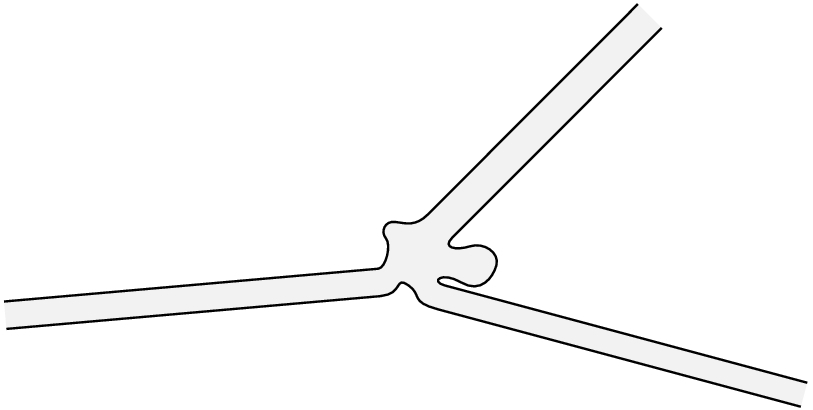
4. The method proposed in the present paper for the construction of asymptotic expansions can be used for the asymptotic investigation of boundary-value problems in graph-junctions of thin domains (Fig. 5), or graph-junctions of thin perforated domains with rapidly varying thickness. In the last case, it is necessary to add series with rapidly oscillating coefficients to the regular part of the asymptotics (see [17]).

Fig. 5.

A graph-junction of thin domains with a local joint.

References

[1]

N.S.

Bakhvalov and

G.P.

Panasenko, Homogenization: Averaging Processes in Periodic Media, Nauka, Moscow, 1984 (in Russian); English translation: Kluwer, Dordrecht/Boston/London, 1989.

[2]

Blanchard and

Gaudiello, Homogenization of highly oscillating boundaries and reduction of dimension for a monotone problem, ESAIM Control. Optim. Calc. Var. 9 (2003), 449–460.

[3]

Blanchard,

Gaudiello and

T.A.

Mel’nyk, Boundary homogenization and reduction of dimension in a Kirchhoff–Love plate, SIAM J. Math. Anal. 39 (2008), 1764–1787.

[4]

A.O.

Borisyuk, Experimental study of wall pressure fluctuations in rigid and elastic pipes behind an axisymmetric narrowing, Journal of Fluids and Structures 26 (2010), 658–674.

[5]

Cardone,

Corbo-Esposito and

Panasenko, Asymptotic partial decomposition for diffusion with sorption in thin structures, Nonlinear Analysis 65 (2006), 79–106.

[6]

G.A.

Chechkin,

V.V.

Jikov,

Lukkassen and

A.L.

Piatnitski, On homogenization of networks and junctions, Asymptotic Analysis 30 (2002), 61–80.

[7]

G.A.

Chechkin and

T.A.

Mel’nyk, Spatial-skin effect for eigenvibrations of a thick cascade junction with “heavy” concentrated masses, Mathematical Methods in Applied Sciences 37 (2014), 56–74.

[8]

Cioranescu,

Saint and

Paulin, Homogenization of Reticulated Structures, Appl. Math. Sci., Vol. 139, Springer-Verlag, New York, 1999.

[9]

De Maio,

Durante and

T.A.

Mel’nyk, Asymptotic approximation for the solution to the Robin problem in a thick multi-level junction, Mathematical Models and Methods in Applied Sciences 15 (2005), 1897–1921.

10.

[10]

Gaudiello and

A.G.

Kolpakov, Influence of non degenerated joint on the global and local behavior of joined rods, International Journal of Engineering Science 49 (2010), 295–309.

11.

[11]

Gaudiello and

Zappale, Junction in a thin multidomain for a fourth order problem, Mathematical Models and Methods in Applied Sciences 16 (2006), 1887–1918.

12.

[12]

A.M.

Il’in, Matching of Asymptotic Expansions of Solutions of Boundary Value Problems, Translations of Mathematical Monographs, Vol. 102, American Mathematical Society, Providence, RI, 1992.

13.

[13]

A.V.

Klevtsovskiy and

T.A.

Mel’nyk, Asymptotic expansions of the solution of an elliptic boundary-value problem for a thin cascade domain, Nonlinear Oscillations 16 (2013), 214–237, English translation: J. Math. Sci.198 (2014), 303–327.

14.

[14]

T.A.

Mel’nyk, Homogenization of the Poisson equation in a thick periodic junction, Zeitschrift für Analysis und ihre Anwendungen 18 (1999), 953–975.

15.

[15]

T.A.

Mel’nyk, Asymptotic approximation for the solution to a semi-linear parabolic problem in a thick junction with the branched structure, J. Math. Anal. Appl. 424 (2015), 1237–1260.

16.

[16]

T.A.

Mel’nyk and

S.A.

Nazarov, Asymptotic structure of the spectrum of the Neumann problem in a thin comb-like domain, C. R. Acad. Sci., Paris 319 (1994), 1343–1348.

17.

[17]

T.A.

Mel’nyk and

A.V.

Popov, Asymptotic analysis of boundary-value and spectral problems in thin perforated regions with rapidly changing thickness and different limiting dimensions, Matem. Sbornik 203 (2012), 97–124, English translation: Sbornik: Mathematics203 (2012), 1169–1195.

18.

[18]

S.A.

Nazarov, Junctions of singularly degenerating domains with different limit dimensions, J. Math. Sci. 80 (1996), 1989–2034.

19.

[19]

S.A.

Nazarov, Asymptotic Theory of Thin Plates and Rods. Dimension Reduction and Integral Bounds, Nauchnaya Kniga, Novosibirsk, 2002 (in Russian).

20.

[20]

S.A.

Nazarov and

B.A.

Plamenevskii, Asymptotics of the spectrum of the Neumann problem in a singularly degenerate thin domains. I, Algebra i Analiz 2 (1990), 85–111.

21.

[21]

S.A.

Nazarov and

A.S.

Slutskii, Arbitrary plane systems of anisotropic beams, Tr. Mat. Inst. Steklov. 236 (2002), 234–261.

22.

[22]

S.A.

Nazarov and

A.S.

Slutskii, Asymptotic analysis of an arbitrary spatial system of thin rods, Proceedings of the St. Petersburg Mathematically Society 10 (2004), 59–109.

23.

[23]

G.P.

Panasenko, Asymptotic analysis of bar systems, Int. Russian Journal of Math. Phys. 2 (1994), 325–352.

24.

[24]

G.P.

Panasenko, Method of asymptotic partial decomposition of domain, Mathematical Models and Methods in Applied Sciences 8 (1998), 139–156.

25.

[25]

G.P.

Panasenko, Multi-Scale Modelling for Structures and Composites, Springer, Dordrecht, 2005.

26.

[26]

Panasenko, Method of asymptotic partial domain decomposition for non-steady problems: Wave equation on a thin structure, in: Analytic Methods in Interdisciplinary Applications,

V.V.

Mityushev and

Ruzhansky, eds, Springer Proceedings in Mathematics & Statistics, Vol. 116, Springer, Cham, 2015.

27.

[27]

Panasenko and

Pileckas, Asymptotic analysis of the non-steady Navier–Stokes equations in a tube structure. I. The case without boundary-layer in time, Nonlinear Analysis 122 (2015), 125–168.

28.

[28]

Panasenko and

Pileckas, Asymptotic analysis of the non-steady Navier–Stokes equations in a tube structure. II. General case, Nonlinear Analysis 125 (2015), 582–607.

29.

[29]

S.E.

Pastukhova, Homogenization of non-linear elasticity problems for thin periodic structures, Doklady RAN 383 (2002), 596–600.

30.

[30]

V.V.

Zhikov, Homogenization of elasticity problems on singular structures, Izv. Math. 66 (2002), 299–365.

31.

[31]

V.V.

Zhikov and

S.E.

Pastukhova, Homogenization of elasticity problems on periodic grids of critical thickness, Matem. Sbornik 194 (2003), 61–96.