Asymptotic approximations elucidating the Gibbs phenomenon and Fejér averaging

Abstract

This paper deals with two trigonometric sums that are pervasive in the literature dealing with the Gibbs phenomenon. In particular, the two sums often serve as test cases for methods – such as the method of Fejér averaging – that aim to overcome the Gibbs phenomenon. Each of the two is the partial sum of a convergent infinite series with a discontinuous limit function. Our starting points are some recently-published results, both exact and asymptotic, for the two sums. For the case of a large number of terms, we proceed from those results to develop simple and revealing asymptotic formulas for the two sums and, also, for their Fejér averages. These formulas break down as we approach the point of discontinuity, so we further develop similar formulas that are appropriate near the discontinuity point. We repeat all these tasks for a third sum whose corresponding infinite series exhibits a logarithmic singularity. Our asymptotic results, which view the three sums from a new perspective, illuminate many aspects of the Gibbs phenomenon and the Fejér averaging method. As an illustrative example of the applicability of our formulas, we exploit their properties to develop a convergence acceleration method. We then use this method to accelerate some (more complicated) sums that exhibit logarithmic singularities, including a sum that arises in several physics applications.

Keywords

Fourier series Gibbs phenomenon Fejér averaging trigonometric sums

1. Introduction

The Gibbs phenomenon (also called Gibbs–Wilbraham phenomenon) occurs when a function with jump discontinuities is expanded into a Fourier series: the partial sums of such series present a characteristic oscillatory behavior and exhibit a slow and non-uniform convergence. Similar phenomena occur in expansions other than Fourier series (such as Fourier-integral expansions, and spline- and wavelet- approximations) that are not of interest herein. The Gibbs phenomenon was noticed by 19th-century experimental physicists, who mistakenly attributed it to imperfections in the measuring instruments [39]; it was also observed experimentally during the early development of radar [27]. Today, the Gibbs phenomenon is relevant to many areas of science and engineering [30], examples being diffraction in digital optics [28], the design of filters in signal processing [34], array synthesis in antenna engineering [1], Magnetic Resonance Imaging [9], shocks in fluid dynamics [4,23], and fronts in meteorology [4]. It is important for the solution of differential equations when using spectral methods [16], as well as finite-element methods [13].

The theoretical study of the Gibbs phenomenon has an interesting and often controversial history [21] (see also [19,24,30]) that began with the works of H. Wilbraham in 1848 and J.W. Gibbs in 1899 (fifty years later than the work of Wilbraham). More recently, textbooks typically introduce the Gibbs phenomenon within the context of simple – but representative – trigonometric expansions of discontinuous functions. As the Gibbs phenomenon is usually (but not always [12]) undesirable, textbooks – as well as a number of recent research papers – often use simple trigonometric sums for a further reason: to design and test methods, such as the method of Fejér averaging, of overcoming or removing the Gibbs phenomenon.

Three such sums are the main focus of the present paper. Although we use them to elucidate the Gibbs phenomenon and Fejér averaging, we do not merely evaluate our sums numerically. Rather, we develop the three sums asymptotically for the case of a large number of terms, and give numerical results that manifest what we believe is an instructive interplay between asymptotics and numerics. We specifically discuss the trigonometric sums $\begin{array}{l} (1) & c_{n} (θ) \equiv \sum_{k = 1}^{n - 1} \frac{cos k θ}{k}, n = 2, 3, 4, \dots, \\ (2) & s_{n} (θ) \equiv \sum_{k = 1}^{n - 1} \frac{sin k θ}{k}, n = 2, 3, 4, \dots, \\ (3) & r_{n} (θ) \equiv \sum_{k = 0}^{n - 1} {(- 1)}^{k} \frac{cos (2 k + 1) θ}{2 k + 1}, n = 1, 2, 3, \dots, \end{array}$ which are the partial sums of the following infinite series [14] $\begin{array}{l} (4) & c_{\infty} (θ) \equiv \sum_{k = 1}^{\infty} \frac{cos k θ}{k} = - ln (2 sin \frac{θ}{2}), 0 < θ < 2 π, \\ (5) & s_{\infty} (θ) \equiv \sum_{k = 1}^{\infty} \frac{sin k θ}{k} = \frac{π - θ}{2}, 0 < θ < 2 π, \\ (6) & r_{\infty} (θ) \equiv \sum_{k = 0}^{\infty} {(- 1)}^{k} \frac{cos (2 k + 1) θ}{2 k + 1} = \{\begin{matrix} π / 4, & | θ | < π / 2, \\ - π / 4, & π / 2 < | θ | < π . \end{matrix} \end{array}$

For reasons obvious from (5) and (6), the $2 π$ -periodic extensions of the infinite series $s_{\infty} (θ)$ and $r_{\infty} (θ)$ , which are discontinuous functions, are often called the “sawtooth-like” and the “square wave” function, respectively [24]. According to J.P. Boyd [5] (ref. [5] is an extended version of [4]), $s_{\infty} (θ)$ “is the prototype for function with discontinuities, which aerodynamicists call ‘shocks’ and meteorologists call ‘fronts’.” The corresponding finite sums $s_{n} (θ)$ and $r_{n} (θ)$ are ubiquitous in textbooks [10,16,24,25,29,36,42] and journal articles [2,12,17,19,21,37] that deal with the Gibbs phenomenon.1

¹
In the Gibbs literature, also ubiquitous is the sum $s_{n}^{'} (θ) \equiv \sum_{k = 1}^{n - 1} {(- 1)}^{k + 1} sin k θ / k$ , whose corresponding infinite series is called the “sawtooth” function; see also [8,27]. Since $s_{n}^{'} (θ) = s_{n} (π - θ)$ , all our results regarding $s_{n} (θ)$ can be rephrased in terms of $s_{n}^{'} (θ)$ .

Specifically, numerically-obtained graphs of

s_{n} (θ)

and

r_{n} (θ)

are frequently used to introduce and illustrate the Gibbs phenomenon [2,10,16,17,19,21,24,25,29,36]; in this regard, much of post-1980 literature [17,19,24,25,36] closely follows the excellent historical article by E. Hewitt and R.E. Hewitt [21].

Most derivations in this work are elementary and have as their starting points some recently-published [14] exact and asymptotic results that we review in Section 2.2

The results of [14] that are reviewed in Section 2 herein concern the sums $c_{n} (θ)$ , $s_{n} (θ)$ , and $r_{n} (θ)$ . Ref. [14] also discusses the partial sum $\sum_{k = 0}^{n - 1} sin [(2 k + 1) θ] / (2 k + 1)$ , which is the means of illustrating the Gibbs phenomenon in several works [6,20,30,33,38–40]. Ref. [14] further discusses the partial sum of $\sum_{k = 1}^{\infty} {(- 1)}^{k + 1} cos k θ / k$ ; this summable infinite series is referred to as the lowest non-Bernoulli Lanczos–Krylov function, or Clausen function [3]. Many of the results in the present paper can be extended to these two partial sums, but we will not do so for brevity.

Our first goal is to present revealing large-n asymptotic approximations for

s_{n} (θ)

and

r_{n} (θ)

. We will call these approximations “large-n (far) formulas.” We also develop a large-n (far) formula for

c_{n} (θ)

, whose limit function is logarithmically singular (rather than discontinuous), see (4). J.P. Boyd has remarked that “A logarithmic singularity is Gibbs Phenomenon with a vengeance!” [3]. As we will see, the large-n (far) formulas enable us to cast a unusual light on the well-known Gibbs phenomenon. However, these formulas break down as we approach the anomaly points (namely,

θ = 0

and

2 π

in the case of

c_{n} (θ)

and

s_{n} (θ)

, and

θ = \pm π / 2

in the case of

r_{n} (θ)

). Accordingly, our second goal is to develop similar approximations, termed “large-n (near) formulas,” that are appropriate near the anomaly points.

The sums $s_{n} (θ)$ and $r_{n} (θ)$ seem to be the most usual test cases for methods aiming to overcome the Gibbs phenomenon; in other words, the effectiveness of such methods is judged by application to $s_{n} (θ)$ or $r_{n} (θ)$ [4,5,10,17–19,29,40]. Perhaps the simplest such method is the method of Fejér averaging [17,20,24,29,42], which can be interpreted as a first-order filter [17] and is the special case $(C, 1)$ of the Cesàro sum $(C, α)$ [24,42]. The method consists of replacing the sequence of partial sums by the sequence of their averages. The third goal of this paper is to compare, in detail, the aforementioned asymptotic approximations for $s_{n} (θ)$ and $r_{n} (θ)$ to corresponding approximations for the Fejér averages $s_{n}^{F} (θ)$ and $r_{n}^{F} (θ)$ . This comparison is illuminating because the large-n (near) formulas capture the first few overshoots and undershoots of $s_{n} (θ)$ and $r_{n} (θ)$ , and demonstrate the lack of overshoots and undershoots in $s_{n}^{F} (θ)$ and $r_{n}^{F} (θ)$ . The large-n (far) formulas, on the other hand, have to do with oscillations or lack of oscillations away from the discontinuity points. We thus apply Fejér averaging to the usual test cases in order to examine them from a different perspective, namely through the lens of asymptotics – Fejér averaging is typically discussed [20,24,29] via the so-called Fejér kernel and numerical results. We repeat this task for the logarithmically singular – and less usual – case of $c_{n} (θ)$ and the corresponding $c_{n}^{F} (θ)$ .

Ours is certainly not the first work that uses asymptotics to illuminate issues related to the Gibbs phenomenon: certain formulas derived herein are connected to ones that can be found in the literature. We discuss such connections (which pertain to $s_{n} (θ)$ and $r_{n} (θ)$ , but not to $c_{n} (θ)$ , nor to $s_{n}^{F} (θ)$ , $r_{n}^{F} (θ)$ , $c_{n}^{F} (θ)$ ) in Section 3.3. For now, let us quote a well-known and informative asymptotic result, adapted from eq. (3.14a) of the book [16] by D. Gottlieb and S.A. Orszag (see also Section 3.3 of A.J. Jerri’s book [24]) to which we will compare our large-n (near) asymptotics: Let $q_{\infty} (θ)$ be a $2 π$ -periodic, piecewise continuous function with bounded total variation, and let $q_{n} (θ) = \sum_{k = - (n - 1)}^{n - 1} α_{k} e^{i k θ}$ be the partial sum of the Fourier series of $q_{\infty} (θ)$ so that $α_{k} = {(2 π)}^{- 1} \int_{0}^{2 π} q_{\infty} (θ) e^{- i k θ} d θ$ . Let $θ_{0}$ be a point of discontinuity of $q_{\infty} (θ)$ . Then for fixed x, $\begin{array}{l} (7) & q_{n} (θ_{0} + \frac{x}{n - \frac{1}{2}}) \sim \frac{1}{2} [q_{\infty} (θ_{0}^{+}) + q_{\infty} (θ_{0}^{-})] + \frac{1}{π} [q_{\infty} (θ_{0}^{+}) - q_{\infty} (θ_{0}^{-})] Si (x), as n \to \infty, \end{array}$ where Si is the Sine integral. We will be interested in the special case where $q_{\infty} (θ_{0}^{+}) = - q_{\infty} (θ_{0}^{-})$ , which is true for both $s_{\infty} (θ)$ and $r_{\infty} (θ)$ . In that case, (7) manifests the Gibbs phenomenon in the following sense (see [16] or Theorem F of [21]): Since the first maximum of $Si (x)$ occurs at $x = π$ , it is a consequence of (7) that, asymptotically, the magnitude of the first overshoot (above or below the right value $q_{\infty} (θ_{0}^{+})$ ) is $[2Si (π) / π - 1] | q_{\infty} (θ_{0}^{+}) |$ , or 17.9% of $| q_{\infty} (θ_{0}^{+}) |$ (according to E. Hewitt and R.E. Hewitt [21], this percentage had been misreported in the pre-1980 literature). In a similar manner, the first undershoot will asymptotically occur when $x = 2 π$ , which is the location of the first minimum of $Si (x)$ .

2. Background

Our starting points are the following results from [14]: Let $λ_{n} (θ)$ and $μ_{n} (θ)$ be the integrals $\begin{array}{l} (8) & λ_{n} (θ) \equiv \int_{0}^{\infty} e^{- n u} \frac{cos θ e^{- u} - 1}{e^{- 2 u} - 2 cos θ e^{- u} + 1} d u, \\ (9) & μ_{n} (θ) \equiv \int_{0}^{\infty} e^{- n u} \frac{- sin θ e^{- u}}{e^{- 2 u} - 2 cos θ e^{- u} + 1} d u . \end{array}$ Then the “remainders” $c_{n} (θ) - c_{\infty} (θ)$ , $s_{n} (θ) - s_{\infty} (θ)$ , and $r_{n} (θ) - r_{\infty} (θ)$ can be expressed in terms of the auxiliary functions $λ_{n} (θ)$ and $μ_{n} (θ)$ as follows: $\begin{array}{l} (10) & c_{n} (θ) - c_{\infty} (θ) = λ_{n} (θ) cos n θ - μ_{n} (θ) sin n θ, 0 < θ < 2 π, \\ (11) & s_{n} (θ) - s_{\infty} (θ) = λ_{n} (θ) sin n θ + μ_{n} (θ) cos n θ, 0 < θ < 2 π, \\ (12) & r_{n} (θ) - r_{\infty} (θ) = \frac{{(- 1)}^{n}}{2} \{\begin{matrix} [- λ_{2 n} (\frac{π}{2} - θ) + λ_{2 n} (\frac{π}{2} + θ)] sin 2 n θ \\ + [μ_{2 n} (\frac{π}{2} - θ) + μ_{2 n} (\frac{π}{2} + θ)] cos 2 n θ \end{matrix}\}, | θ | < π / 2 . \end{array}$ Furthermore, the auxiliary functions $λ_{n} (θ)$ and $μ_{n} (θ)$ possess the following asymptotic power series (Poincaré asymptotic expansions): $\begin{array}{l} (13) & λ_{n} (θ) = - \frac{1}{2 n} - {csc}^{2} \frac{θ}{2} \frac{1}{4 n^{2}} + (2 + cos θ) {csc}^{4} \frac{θ}{2} \frac{1}{8 n^{4}} + O (\frac{1}{n^{6}}), as n \to \infty, \\ (14) & μ_{n} (θ) = - cot \frac{θ}{2} \frac{1}{2 n} + cot \frac{θ}{2} {csc}^{2} \frac{θ}{2} \frac{1}{4 n^{3}} + O (\frac{1}{n^{5}}), as n \to \infty . \end{array}$ In (13) and (14), we have written the first few terms of the full asymptotic expansions (provided in [14] in terms of the Eulerian numbers [33], but not of interest herein) of $λ_{n} (θ)$ and $μ_{n} (θ)$ . Together, eqns. (10)–(14) form “compound asymptotic expansions” – in the sense discussed in [41] and [15] – of $c_{n} (θ)$ , $s_{n} (θ)$ , and $r_{n} (θ)$ [14].

It is worth noting that (8)–(12) are different from the usual integral representations, involving the Dirichlet kernel, for the partial sums of Fourier series [10,42].

3. Asymptotic approximations for $c_{n} (θ)$ , $s_{n} (θ)$ , and $r_{n} (θ)$

3.1. Large-n (far) formulas

Our large-n (far) formulas come from the first few terms in the compound asymptotic expansions of (10)–(14). These are $\begin{array}{l} (15) & \begin{aligned} c_{n} (θ) = - ln (2 sin \frac{θ}{2}) + \frac{sin [(n - \frac{1}{2}) θ]}{2 n sin (\frac{θ}{2})} - \frac{cos n θ}{2 n^{2} (1 - cos θ)} \\ + O (\frac{1}{n^{3}}), as n \to \infty (0 < θ < 2 π), \end{aligned} \\ (16) & s_{n} (θ) = \frac{π - θ}{2} - \frac{cos [(n - \frac{1}{2}) θ]}{2 n sin (\frac{θ}{2})} - \frac{sin n θ}{2 n^{2} (1 - cos θ)} + O (\frac{1}{n^{3}}), as n \to \infty (0 < θ < 2 π), \\ (17) & r_{n} (θ) = \frac{π}{4} - \frac{{(- 1)}^{n} cos 2 n θ}{4 n cos θ} + \frac{{(- 1)}^{n} sin θ sin 2 n θ}{8 n^{2} {cos}^{2} θ} + O (\frac{1}{n^{3}}), as n \to \infty (| θ | < \frac{π}{2}) . \end{array}$

In the right-hand sides of (15)–(17), the first terms are $O (1)$ and are equal to the values $c_{\infty} (θ)$ , $s_{\infty} (θ)$ , and $r_{\infty} (θ)$ . The terms that follow are $O (1 / n)$ or, to be more precise, they consist of oscillating functions (e.g. ${(- 1)}^{n} cos 2 n θ$ in the case of $r_{n} (θ)$ ) times $O (1 / n)$ -functions. The next terms and the remainders are $O (1 / n^{2})$ and $O (1 / n^{3})$ in the same sense.

It is logical to expect that (15) and (16) become less accurate as θ approaches 0 or $2 π$ ; the same applies for (17) for θ close to $\pm π / 2$ . In other words [22], the pointwise asymptoticness in n is nonuniform in θ. We will thus refer to (15)–(17) as “large-n (far) formulas,” as they better describe the region which is far from the discontinuity or logarithmic singularity. These formulas, which are written – to $O (1 / n)$ only – in the middle row of Table 1, cannot accurately describe the overshoots and undershoots very close to the point of anomaly.

Table 1
Asymptotic formulas for $c_{n} (θ)$ , $s_{n} (θ)$ , and $r_{n} (θ)$

$c_{n} (θ)$ (logarithmic case) $s_{n} (θ)$ (discontinuous case) $r_{n} (θ)$ (discontinuous case)

Exact $\sum_{k = 1}^{n - 1} \frac{cos k θ}{k}$ $\sum_{k = 1}^{n - 1} \frac{sin k θ}{k}$ $\sum_{k = 0}^{n - 1} {(- 1)}^{k} \frac{cos (2 k + 1) θ}{2 k + 1}$

Large- n (far) $- ln (2 sin \frac{θ}{2}) + \frac{sin (N θ)}{2 n sin (θ / 2)}$ $\frac{π - θ}{2} - \frac{cos (N θ)}{2 n sin (θ / 2)}$ $\frac{π}{4} - \frac{{(- 1)}^{n} cos 2 n θ}{4 n cos θ}$

$(0 < θ < 2 π)$ $(0 < θ < 2 π)$ $(- π / 2 < θ < π / 2)$

Large- n (near) $- ln θ + Ci (N θ)$ , $Si (N θ) - \frac{θ}{2}$ $\frac{1}{2} Si (N^{'} ϕ) + \frac{ϕ}{4} \frac{sin N^{'} ϕ}{N^{'} ϕ}$

θ small and positive θ small and positive θ close to and less than $π / 2$

	$c_{n} (θ)$ (logarithmic case)	$s_{n} (θ)$ (discontinuous case)	$r_{n} (θ)$ (discontinuous case)
Exact	$\sum_{k = 1}^{n - 1} \frac{cos k θ}{k}$	$\sum_{k = 1}^{n - 1} \frac{sin k θ}{k}$	$\sum_{k = 0}^{n - 1} {(- 1)}^{k} \frac{cos (2 k + 1) θ}{2 k + 1}$
Large- n (far)	$- ln (2 sin \frac{θ}{2}) + \frac{sin (N θ)}{2 n sin (θ / 2)}$	$\frac{π - θ}{2} - \frac{cos (N θ)}{2 n sin (θ / 2)}$	$\frac{π}{4} - \frac{{(- 1)}^{n} cos 2 n θ}{4 n cos θ}$
$(0 < θ < 2 π)$	$(0 < θ < 2 π)$	$(- π / 2 < θ < π / 2)$
Large- n (near)	$- ln θ + Ci (N θ)$ ,	$Si (N θ) - \frac{θ}{2}$	$\frac{1}{2} Si (N^{'} ϕ) + \frac{ϕ}{4} \frac{sin N^{'} ϕ}{N^{'} ϕ}$
θ small and positive	θ small and positive	θ close to and less than $π / 2$

Notation: $N \equiv n - \frac{1}{2}$ , $N^{'} \equiv 2 n - \frac{1}{2}$ , $ϕ \equiv \frac{π}{2} - θ$ .

3.2. Large-n (near) formulas

We now find formulas (“large-n (near) formulas”) suitable for the aforementioned purpose. Consider $c_{n} (θ)$ and $s_{n} (θ)$ first. For reasons to become apparent, we define $\begin{matrix} (18) & N \equiv n - \frac{1}{2}, \end{matrix}$ and take the limit $\begin{matrix} (19) & N \to \infty, θ \to 0, N θ = fixed (θ > 0) . \end{matrix}$ In terms of N, and setting $u = θ x$ , eqs. (8)–(11) can be re-written to give $\begin{array}{l} (20) & c_{n} (θ) - c_{\infty} (θ) = - ξ_{N} (θ) cos N θ + ρ_{N} (θ) sin N θ, \\ (21) & s_{n} (θ) - s_{\infty} (θ) = - ξ_{N} (θ) sin N θ - ρ_{N} (θ) cos N θ, \end{array}$ where $\begin{array}{l} (22) & ξ_{N} (θ) \equiv \int_{0}^{\infty} e^{- N θ x} θ cos \frac{θ}{2} \frac{sinh (θ x / 2)}{cosh (θ x) - cos θ} d x, \\ (23) & ρ_{N} (θ) \equiv \int_{0}^{\infty} e^{- N θ x} θ sin \frac{θ}{2} \frac{cosh (θ x / 2)}{cosh (θ x) - cos θ} d x . \end{array}$ The quantities respectively multiplying the exponentials in (22) and (23) satisfy $\begin{array}{l} (24) & θ cos \frac{θ}{2} \frac{sinh (θ x / 2)}{cosh (θ x) - cos θ} = \frac{x}{1 + x^{2}} - \frac{x}{24} θ^{2} + O (θ^{4}), as θ \to 0, \\ (25) & θ sin \frac{θ}{2} \frac{cosh (θ x / 2)}{cosh (θ x) - cos θ} = \frac{1}{1 + x^{2}} + \frac{1}{24} θ^{2} + O (θ^{4}), as θ \to 0 . \end{array}$ Therefore, term-by-term integration, together with use of the integrals [33, Sections 6.2.19, 6.2.20, 6.7.13, 6.7.14] $\begin{array}{l} (26) & - cos N θ \int_{0}^{\infty} e^{- N θ x} \frac{x}{1 + x^{2}} d x + sin N θ \int_{0}^{\infty} e^{- N θ x} \frac{1}{1 + x^{2}} d x = Ci (N θ), \\ (27) & - sin N θ \int_{0}^{\infty} e^{- N θ x} \frac{x}{1 + x^{2}} d x - cos N θ \int_{0}^{\infty} e^{- N θ x} \frac{1}{1 + x^{2}} d x = Si (N θ) - \frac{π}{2}, \end{array}$ give $\begin{array}{l} (28) & c_{n} (θ) - c_{\infty} (θ) \sim Ci (N θ) + \frac{θ^{2}}{24} (\frac{sin N θ}{N θ} + \frac{cos N θ}{{(N θ)}^{2}}), \\ (29) & s_{n} (θ) - s_{\infty} (θ) \sim Si (N θ) - \frac{π}{2} + \frac{θ^{2}}{24} (\frac{sin N θ}{{(N θ)}^{2}} - \frac{cos N θ}{N θ}) . \end{array}$ By re-introducing $s_{\infty} (θ)$ from (5), eq. (29) gives an asymptotic approximation for $s_{n} (θ)$ , correct to $O (θ^{2})$ ; it is written, to $O (θ)$ only, in the last row of Table 1. The corresponding results for $c_{n} (θ)$ are obtained from (28), (4), and $\begin{matrix} (30) & c_{\infty} (θ) = - ln (2 sin \frac{θ}{2}) \sim - ln θ + \frac{θ^{2}}{24} + O (θ^{4}), as θ \to 0 . \end{matrix}$ To find a corresponding formula for $r_{n} (θ)$ , set $\begin{matrix} (31) & ϕ \equiv \frac{π}{2} - θ and N^{'} \equiv 2 n - \frac{1}{2}, \end{matrix}$ and consider the limit $\begin{matrix} (32) & N^{'} \to \infty, ϕ \to 0, N^{'} ϕ = fixed (ϕ > 0) . \end{matrix}$ It is evident from (2) and (3) that $\begin{matrix} (33) & r_{n} (\frac{π}{2} - ϕ) = \frac{1}{2} [s_{2 n} (ϕ) + s_{2 n} (π - ϕ)] . \end{matrix}$ The behavior of the first term on the right-hand side (RHS) of (33) is obtained immediately from Table 1. It is $\begin{matrix} (34) & s_{2 n} (ϕ) \sim Si (N^{'} ϕ) - \frac{ϕ}{2} + \frac{ϕ^{2}}{24} [\frac{sin N^{'} ϕ}{{(N^{'} ϕ)}^{2}} - \frac{cos N^{'} ϕ}{N^{'} ϕ}] . \end{matrix}$ From (5), (21)–(23), and (31) we obtain the following exact expression for the second term on the RHS of (33). $\begin{matrix} (35) & s_{2 n} (π - ϕ) = \frac{ϕ}{2} + ω_{N^{'}} (ϕ) cos N^{'} ϕ + ψ_{N^{'}} (ϕ) sin N^{'} ϕ, \end{matrix}$ where $\begin{array}{l} (36) & ω_{N^{'}} (ϕ) \equiv \int_{0}^{\infty} e^{- N^{'} ϕ x} ϕ sin \frac{ϕ}{2} \frac{sinh (ϕ x / 2)}{cosh (ϕ x) + cos ϕ} d x, \\ (37) & ψ_{N^{'}} (ϕ) \equiv \int_{0}^{\infty} e^{- N^{'} ϕ x} ϕ cos \frac{ϕ}{2} \frac{cosh (ϕ x / 2)}{cosh (ϕ x) + cos ϕ} d x . \end{array}$ Since $\begin{array}{l} (38) & ϕ sin \frac{ϕ}{2} \frac{sinh (ϕ x / 2)}{cosh (ϕ x) + cos ϕ} = O (ϕ^{3}), as ϕ \to 0, \\ (39) & ϕ cos \frac{ϕ}{2} \frac{cosh (ϕ x / 2)}{cosh (ϕ x) + cos ϕ} = \frac{ϕ}{2} + O (ϕ^{3}), as ϕ \to 0, \end{array}$ we obtain $\begin{matrix} (40) & s_{2 n} (π - ϕ) = \frac{ϕ}{2} (1 + \frac{sin N^{'} ϕ}{N^{'} ϕ}) + O (ϕ^{3}), as ϕ \to 0 . \end{matrix}$ Eqs. (33), (34), and (40) give, to $O (ϕ^{2})$ , the asymptotic approximation to $r_{n} (θ)$ . The last row of Table 1 shows this result to $O (ϕ)$ .

3.3. Comparisons with formulas in the literature; initial numerical results

In this section, we compare the formulas in Sections 3.1 and 3.2 to some similar formulas in the Gibbs-phenomenon literature. Firstly, the formulas concerning $s_{n} (θ)$ are connected to certain formulas in the book [29] of C. Lanczos: For small θ, (16) agrees (to $O (1 / n^{2})$ ) with eq. (10.6) of [29]. And the first two terms of our large-n (near) formula for $s_{n} (θ)$ (i.e., the quantity $Si (N θ) - θ / 2$ written in Table 1) agree with eq. (10.4) of [29].

Let us now compare with formula (7) (see our Introduction) of D. Gottlieb and S.A. Orszag: Set $q_{\infty} (θ) = s_{\infty} (θ)$ and $θ_{0} = 0$ . It is easy to show that the first term in the RHS of (7) vanishes and that the second reduces to $Si (N θ)$ . Similarly, if we set $q_{\infty} (θ) = r_{\infty} (θ)$ and $θ_{0} = π / 2$ , we see that $q_{2 n} (θ) = r_{n} (θ)$ and that the RHS of (7) reduces to $Si (N^{'} ϕ) / 2$ . For the two discontinuous cases, we have thus shown that the first ( $O (1)$ ) terms of the large-n (near) formulas of Table 1 are the same as those provided by the general asymptotic approximation (7). And, subject to the conditions (19) or (32), we have improved the approximation provided by (7), by means of the additional terms written in Table 1. (In Section 3.2, we obtained yet another term for each of the two cases.)

On the other hand, apart from the term $- ln θ$ (this term is simply the leading term of the small-θ approximation to the limit function $c_{\infty} (θ)$ , see (30)), our large-n (near) formula for $c_{n} (θ)$ seems to be entirely new; we were not even able to find the $O (1)$ term $Ci (N θ)$ – which manifests Gibbs-like overshoots and undershoots in $c_{n} (θ)$ – in the literature.

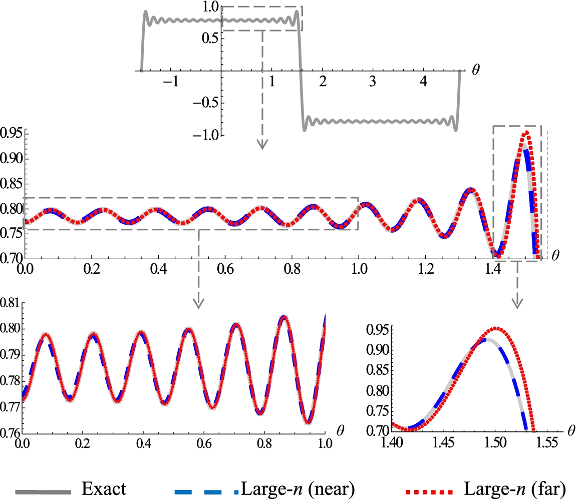
We did many numerical checks to our formulas. Results for $r_{n} (θ)$ and for $n = 20$ are shown in Fig. 1 (results for $c_{n} (θ)$ and $s_{n} (θ)$ are very similar). At the scale of the figure, the exact (i.e., obtained numerically from (3)) curve coincides with the large-n (near) curve close to $θ = π / 2$ , and coincides with the large-n (far) curve as one moves away from the discontinuity at $θ = π / 2$ .

Fig. 1.

Plots of exact, large-n (near) and large-n (far) approximations of $r_{n} (θ)$ (see Table 1), for $n = 20$ .

The errors in Fig. 1 are seen to be quite small. This smallness is better revealed in Fig. 2, which gives percentage errors for each of the two formulas. All errors remain less than 1% throughout the entire range of the figure, and – just as expected – each approximation improves as we approach its region of validity. The errors exhibit an oscillatory behavior that appears quite interesting. They can be approximated by the next terms we have determined.

Fig. 2.

Plots of errors for the large-n (near) and large-n (far) approximations of $r_{n} (θ)$ , for $n = 20$ .

The large-n (near) formulas can therefore capture the first few overshoots and undershoots with excellent accuracy, while the large-n (far) formulas have to do with oscillations far from the discontinuity points. We defer further discussions of Table 1 until Section 5, as the formulas of Table 1 are better comprehended if compared to corresponding ones pertaining to the Fejér averages of $s_{n} (θ)$ , $c_{n} (θ)$ , and $r_{n} (θ)$ .

4. Asymptotic approximations for Fejér averages

4.1. Definitions

The Fejér averages $s_{n}^{F} (θ)$ and $c_{n}^{F} (θ)$ of $s_{n} (θ)$ and $c_{n} (θ)$ are defined by the usual relations $\begin{array}{l} (41) & s_{n}^{F} (θ) \equiv \frac{1}{n - 1} \sum_{k = 2}^{n} s_{k} (θ), n = 2, 3, 4, \dots, \\ (42) & c_{n}^{F} (θ) \equiv \frac{1}{n - 1} \sum_{k = 2}^{n} c_{k} (θ), n = 2, 3, 4, \dots . \end{array}$ Because $r_{n} (θ)$ has a different lower summation limit than $s_{n} (θ)$ and $c_{n} (θ)$ (0 instead of 1), we define the Fejér averages $r_{n}^{F} (θ)$ of $r_{n} (θ)$ through the somewhat different equation $\begin{matrix} (43) & r_{n}^{F} (θ) \equiv \frac{1}{n} \sum_{k = 1}^{n} r_{k} (θ), n = 1, 2, 3, \dots . \end{matrix}$

4.2. Derivations

We first deal with the asymptotics of $s_{n}^{F} (θ)$ and $c_{n}^{F} (θ)$ . It follows from (1), (2), (41), (42), and the identity $\begin{matrix} (44) & \sum_{k = 2}^{n} \sum_{m = 1}^{k - 1} α_{m} = \sum_{k = 1}^{n - 1} (n - k) α_{k}, n = 2, 3, 4, \dots, \end{matrix}$ that $\begin{matrix} (45) & s_{n}^{F} (θ) = \frac{n}{n - 1} s_{n} (θ) - \frac{1}{n - 1} \sum_{k = 1}^{n - 1} sin k θ, n = 2, 3, 4, \dots \end{matrix}$ and $\begin{matrix} (46) & c_{n}^{F} (θ) = \frac{n}{n - 1} c_{n} (θ) - \frac{1}{n - 1} \sum_{k = 1}^{n - 1} cos k θ, n = 2, 3, 4, \dots . \end{matrix}$ Using the tabulated sums in [26], we can rewrite (45) and (46) as $\begin{matrix} (47) & s_{n}^{F} (θ) = \frac{n}{n - 1} s_{n} (θ) + \frac{1}{n - 1} \frac{cos (N θ) - cos (θ / 2)}{2 sin (θ / 2)}, \end{matrix}$ and $\begin{matrix} (48) & c_{n}^{F} (θ) = \frac{n}{n - 1} c_{n} (θ) - \frac{1}{n - 1} \frac{sin (N θ) - sin (θ / 2)}{2 sin (θ / 2)}, \end{matrix}$ where we introduced the quantity $N \equiv n - 1 / 2$ appearing in (18) and Table 1.

We now turn to $r_{n}^{F} (θ)$ . With (43) and (3), we can obtain an equation analogous to (45) and (46) $\begin{matrix} (49) & r_{n}^{F} (θ) = (1 + \frac{1}{2 n}) r_{n} (θ) - \frac{1}{2 n} \sum_{k = 0}^{n - 1} {(- 1)}^{k} cos [(2 k + 1) θ], n = 1, 2, 3, \dots . \end{matrix}$ Direct evaluation of the sum with the aid of [35, Formula 4.4.1.6] gives $\begin{matrix} (50) & r_{n}^{F} (θ) = (1 + \frac{1}{2 n}) r_{n} (θ) + \frac{{(- 1)}^{n} cos 2 n θ - 1}{4 n cos θ} . \end{matrix}$ The exact equations (47), (48), and (50) express the Fejér averages $s_{n}^{F} (θ)$ , $c_{n}^{F} (θ)$ , and $r_{n}^{F} (θ)$ in terms of elementary functions and the corresponding partial sums $s_{n} (θ)$ , $c_{n} (θ)$ , and $r_{n} (θ)$ themselves. (For more complicated sums, it is usually not possible to obtain expressions of such simplicity.) Note that the said equations explicitly verify that the Fejér averages have the same large-n limit functions as do the partial sums.

By expanding the elementary functions and replacing the partial sums by their asymptotic formulas from Table 1, we easily find corresponding asymptotic formulas for the Fejér averages. We omit details and summarize our findings in Table 2.

Table 2
Asymptotic formulas for Fejér averages of $c_{n} (θ)$ , $s_{n} (θ)$ , and $r_{n} (θ)$

$c_{n}^{F} (θ)$ (logarithmic case) $s_{n}^{F} (θ)$ (discontinuous case) $r_{n}^{F} (θ)$ (discontinuous case)

Exact $\frac{1}{n - 1} \sum_{k = 2}^{n} c_{k} (θ)$ $\frac{1}{n - 1} \sum_{k = 2}^{n} s_{k} (θ)$ $\frac{1}{n} \sum_{k = 1}^{n} r_{k} (θ)$

Large- n (far) $- ln (2 sin \frac{θ}{2}) + \frac{1}{n} [\frac{1}{2} - ln (2 sin \frac{θ}{2})]$ $\frac{π - θ}{2} + \frac{1}{2 n} (π - θ - cot \frac{θ}{2})$ $\frac{π}{4} + \frac{1}{n} (\frac{π}{8} - \frac{1}{4 cos θ})$

$(0 < θ < 2 π)$ $(0 < θ < 2 π)$ $(- π / 2 < θ < π / 2)$

Large- n (near) $\begin{matrix} - ln θ + Ci (N θ) - \frac{sin N θ}{N θ}, \\ θ small and positive \end{matrix}$ $\begin{matrix} Si (N θ) - \frac{1 - cos N θ}{N θ} \\ + θ \frac{cos N θ - {(N θ)}^{2} + 2 (N θ) Si (N θ) - 1}{2 {(N θ)}^{2}}, \\ θ small and positive \end{matrix}$ $\begin{matrix} \frac{1}{2} Si (N^{'} ϕ) - \frac{1 - cos N^{'} ϕ}{2 N^{'} ϕ} \\ + ϕ \frac{1 + 2 (N^{'} ϕ) Si (N^{'} ϕ) - cos N^{'} ϕ}{4 {(N^{'} ϕ)}^{2}}, \\ θ close to and less than π / 2 \end{matrix}$

	$c_{n}^{F} (θ)$ (logarithmic case)	$s_{n}^{F} (θ)$ (discontinuous case)	$r_{n}^{F} (θ)$ (discontinuous case)
Exact	$\frac{1}{n - 1} \sum_{k = 2}^{n} c_{k} (θ)$	$\frac{1}{n - 1} \sum_{k = 2}^{n} s_{k} (θ)$	$\frac{1}{n} \sum_{k = 1}^{n} r_{k} (θ)$
Large- n (far)	$- ln (2 sin \frac{θ}{2}) + \frac{1}{n} [\frac{1}{2} - ln (2 sin \frac{θ}{2})]$	$\frac{π - θ}{2} + \frac{1}{2 n} (π - θ - cot \frac{θ}{2})$	$\frac{π}{4} + \frac{1}{n} (\frac{π}{8} - \frac{1}{4 cos θ})$
$(0 < θ < 2 π)$	$(0 < θ < 2 π)$	$(- π / 2 < θ < π / 2)$
Large- n (near)	$\begin{matrix} - ln θ + Ci (N θ) - \frac{sin N θ}{N θ}, \\ θ small and positive \end{matrix}$	$\begin{matrix} Si (N θ) - \frac{1 - cos N θ}{N θ} \\ + θ \frac{cos N θ - {(N θ)}^{2} + 2 (N θ) Si (N θ) - 1}{2 {(N θ)}^{2}}, \\ θ small and positive \end{matrix}$	$\begin{matrix} \frac{1}{2} Si (N^{'} ϕ) - \frac{1 - cos N^{'} ϕ}{2 N^{'} ϕ} \\ + ϕ \frac{1 + 2 (N^{'} ϕ) Si (N^{'} ϕ) - cos N^{'} ϕ}{4 {(N^{'} ϕ)}^{2}}, \\ θ close to and less than π / 2 \end{matrix}$

Notation: $N \equiv n - \frac{1}{2}$ , $N^{'} \equiv 2 n - \frac{1}{2}$ , $ϕ \equiv \frac{π}{2} - θ$ .

To the best of our knowledge, all formulas in Table 2 are new.

5. Describing Fejér averaging and the Gibbs phenomenon via asymptotics

A comparison between Tables 1 and 2 reveals the following features:

5.1. Fejér averaging eliminates dominant oscillations, but preserves the order of the error

In the large-n (far) formulas, the effect of Fejér averaging is to replace the oscillatory terms of $O (1 / n)$ by non-oscillatory terms of the same order; in the case of $r_{n} (θ)$ , for instance, $- {(- 1)}^{n} cos (2 n θ) / (4 n cos θ)$ is replaced by $(\frac{π}{8} - \frac{1}{4 cos θ}) / n$ . Thus, the leading term of the error in the large-n (far) formulas in Table 2 is truly $O (1 / n)$ , not an oscillating function times a $O (1 / n)$ -function (as in Table 1). This means that, far from the anomaly and for sufficiently large n, the Fejér averages oscillate less than do the sums themselves. In this sense, Fejér averaging “reduces the Gibbs phenomenon” in the two discontinuous cases. A similar remark is true for the logarithmic case.

5.2. “Asymptotic intersection points” of Fejér averages

As discussed above, Fejér averaging eliminates the dominant oscillations. However, it is apparent (e.g., from (17) and (50)) that the Fejér averages will still exhibit oscillations, arising from higher order terms. Any such oscillations, however, need not be centered around the final (at $n = \infty$ ) value (namely $r_{\infty} (θ) = π / 4$ in the case of $r_{n}^{F} (θ)$ , or $s_{\infty} (θ) = (π - θ) / 2$ in the case of $s_{n}^{F} (θ)$ ). In the case of $r_{n}^{F} (θ)$ , the $O (1 / n)$ term in the large-n (far) formula vanishes twice in the interval $(- π / 2, π / 2)$ , specifically when $\begin{matrix} (51) & θ = \pm θ_{ip} where θ_{ip} = Arccos (2 / π) ≅ 0.881 rad . \end{matrix}$ For large n, these two points are roughly where the plot of $r_{n}^{F} (θ)$ will intersect the horizontal line $r_{\infty} (θ) = π / 4$ . Similar discussions can be made for the cases of $s_{n}^{F} (θ)$ (here, we will have three “asymptotic intersection points” in $(0, 2 π)$ ) and $c_{n}^{F} (θ)$ (two such points in $(0, 2 π)$ , for which formulas similar to (51) can be derived). For the two discontinuous cases, the fact that there are few intersection points means that Fejér averaging “reduces the Gibbs phenomenon” in yet another sense. (A more precise statement of the “reduction” is given in Sections II.9 and III.11 of A. Zygmund’s treatise [42], where the Gibbs phenomenon is defined in a rigorous manner.)

5.3. Values of Fejér averages at first overshoot and undershoot

When the sums themselves overshoot/undershoot, what are the values of their Fejér averages? For the first few overshoots/undershoots, this question can be addressed via the large-n (near) formulas and, in particular, the $O (1)$ term in the two discontinuous cases. The effect of Fejér averaging is to replace the $Si (x)$ of Table 1, where $x = N θ$ or $x = N^{'} ϕ$ , by $Si (x) - (1 - cos x) / x$ . The latter function equals $Si (π) - 2 / π ≅ 1.22$ when $x = π$ and remains unaltered (and equal to $Si (2 π)$ ) when $x = 2 π$ . For sufficiently large n, therefore, when the first overshoot occurs, i.e. where $r_{n} (θ)$ overshoots $r_{\infty} (π / 2 -)$ by $2Si (π) / π - 1 ≅ 17.9 %$ (see our Introduction), $r_{n}^{F} (θ)$ will be less than the value $r_{\infty} (π / 2 -)$ by $\begin{matrix} (52) & | 2 (Si (π) - 2 / π) / π - 1 | ≅ 23 % . \end{matrix}$ When the first undershoot of $r_{n} (θ)$ occurs, $r_{n} (θ)$ and $r_{n}^{F} (θ)$ will be roughly equal, viz., $\begin{matrix} (53) & r_{n} (θ) ≅ r_{n}^{F} (θ) \end{matrix}$ in the sense that $r_{n} (θ) - r_{n}^{F} (θ) = O (1 / n^{2})$ when θ is such that $x = 2 π$ . The same statements – as well as (52) and (53) – remain true for $s_{n}^{F} (θ)$ .

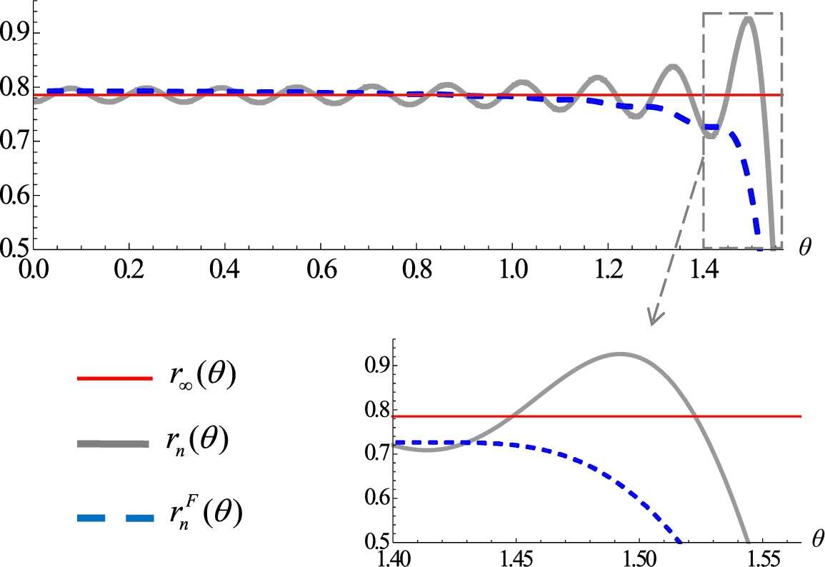
5.4. Numerical illustrations of asymptotic predictions

All features discussed in Sections 5.1–5.3 are illustrated in Fig. 3, in which $r_{\infty} (θ) = π / 4$ is shown together with $r_{n} (θ)$ and $r_{n}^{F} (θ)$ , as calculated numerically from (3) and (43), for $n = 20$ . The graph of $r_{n}^{F} (θ)$ has barely visible oscillations and only intersects the line $r_{\infty} (θ) = π / 4$ once, at $θ = 0.880$ rad (instead of $θ = θ_{ip} ≅ 0.881$ rad predicted asymptotically from (51)). The first overshoot at right occurs when $θ =$ 1.492 rad (the value predicted asymptotically, i.e., when $N^{'} ϕ = π$ , is 1.491 rad) and $r_{n} (1.492)$ is 17.9% of the value $π / 4 = 0.7854$ (exactly as predicted asymptotically). When $θ =$ 1.492 rad, we have $r_{n}^{F} (1.492) = 0.6317$ , which is 19.5% less than the value $π / 4 = 0.7854$ (close to the 23% predicted asymptotically from (52)). The first undershoot at right occurs when $θ = 1.414$ rad (the value predicted asymptotically, i.e., when $N^{'} ϕ = 2 π$ , is 1.411 rad). When $θ = 1.414$ rad, we have $r_{n} (1.414) = 0.7088$ and $r_{n}^{F} (1.414) = 0.7264$ , and these two values are within 2.5% of one another (asymptotically, they are predicted by (53) to be equal).

We performed many numerical investigations; as expected, for larger values of n, the agreement with the asymptotic predictions became even better.

Fig. 3.

Plots of $r_{\infty} (θ)$ , $r_{n} (θ)$ , and $r_{n}^{F} (θ)$ , for $n = 20$ , as calculated numerically.

6. Development of a convergence acceleration method

Let $f_{n}$ ( $n = 1, 2, \dots$ ) be a sequence (e.g., the partial sums of an infinite series) that converges to an unknown limit $f_{\infty}$ . A Convergence Acceleration Method (CAM) transforms $f_{n}$ into another sequence $t_{n}$ such that: (i) $t_{n}$ is convergent; (ii) the limit of $t_{n}$ is $f_{\infty}$ , i.e., the original and transformed sequences have the same limit; (iii) $t_{n}$ converges faster to $f_{\infty}$ than does $f_{n}$ . There exist very many CAMs in the literature (see, for example, [7]); each is defined by a specific rule giving the transformed sequence elements from the original ones, and each accelerates a particular class of sequences $f_{n}$ . In this section, we use our large-n (far) formulas to develop a CAM that, when θ is not very close to 0 or $2 π$ , accelerates the θ-dependent sum $f_{n} = c_{n} (θ)$ (logarithmic case). We then show that our CAM is appropriate for more general θ-dependent sequences.

6.1. CAM for $c_{n} (θ)$

Throughout this section, we follow the convention introduced in Section 3.1: $O (1 / n)$ (or $O (1 / n^{2})$ ) means an oscillating function times a $O (1 / n)$ (or $O (1 / n^{2})$ )-function. Table 1 shows that $c_{n} (θ) - c_{\infty} (θ) = O (1 / n)$ . We seek a $t_{n} (θ)$ in the form $\begin{matrix} (54) & t_{n} (θ) = α c_{n} (θ) + β c_{n - 1} (θ) + γ c_{n - 2} (θ), n = 4, 5, \dots, \end{matrix}$ (in which α, β, and γ are independent of n) such that $\begin{matrix} (55) & t_{n} (θ) - c_{\infty} (θ) = O (1 / n^{2}) . \end{matrix}$

We write (15) (or see Table 1) and (4) as $\begin{matrix} (56) & c_{n} (θ) = c_{\infty} (θ) + \frac{1}{n} v_{n} (θ) + O (\frac{1}{n^{2}}), \end{matrix}$ where $\begin{matrix} (57) & v_{n} (θ) = \frac{sin [(n - 1 / 2) θ]}{2 sin (θ / 2)} . \end{matrix}$ It is a simple consequence of (56) and (57) that $\begin{matrix} (58) & c_{n - 1} (θ) = c_{\infty} (θ) + \frac{1}{n} v_{n} (θ) cos θ - \frac{1}{n} u_{n} (θ) sin θ + O (\frac{1}{n^{2}}), \end{matrix}$ and $\begin{matrix} (59) & c_{n - 2} (θ) = c_{\infty} (θ) + \frac{1}{n} v_{n} (θ) cos 2 θ - \frac{1}{n} u_{n} (θ) sin 2 θ + O (\frac{1}{n^{2}}), \end{matrix}$ where $\begin{matrix} (60) & u_{n} (θ) = \frac{cos [(n - 1 / 2) θ]}{2 sin (θ / 2)} . \end{matrix}$ Now substitute (56), (58), and (59) into (54) to obtain $t_{n} (θ)$ as a linear combination of $c_{\infty} (θ)$ , $u_{n} (θ)$ , and $v_{n} (θ)$ (plus terms of $O (1 / n^{2})$ ). This $t_{n} (θ)$ will satisfy (55) if the respective coefficients are 1, 0, and 0. These three requirements yield a linear system of equations for α, β, and γ. The solution of the system is $\begin{matrix} (61) & α = γ = \frac{1}{2 (1 - cos θ)}, β = \frac{- cos θ}{1 - cos θ} . \end{matrix}$ Combining (61) and (54), and writing $f_{n} (θ)$ in place of $c_{n} (θ)$ for later convenience, the desired CAM is seen to be $\begin{matrix} (62) & t_{n} (θ) = \frac{f_{n} (θ) - 2 cos θ f_{n - 1} (θ) + f_{n - 2} (θ)}{2 (1 - cos θ)}, n = 4, 5, \dots . \end{matrix}$

For $θ = 0$ and $θ = 2 π$ , the denominator in (62) vanishes while the numerator generally does not. Consequently, we can only expect (62) to work far from $θ = 0$ and $θ = 2 π$ ; this is consistent with the fact that (62) was derived from the large-n (far) formulas. We stress that we were able to obtain (62) because of the specific form of the large-n (far) formulas, see (56) and (57). By contrast, it is impossible to find a CAM in the form (54) (with α, β, γ independent of n) that can work for the case of the large-n (near) formulas.

Although we used the language of CAMs and extrapolation methods, it is evident that (62) can be viewed as a means of reducing the Gibbs phenomenon, just like the method of Fejér averaging. For the case $f_{n} (θ) = c_{n} (θ)$ (and for θ far from 0 and $2 π$ ), (62) is a superior method because the order of the leading term of the error is smaller – compare (55) to the discussions in Section 5.1. In the next section, we will present numerical results supporting this.

6.2. Applicability of the CAM to other sums; test cases

The CAM (62) is suitable for sums other than $f_{n} (θ) = c_{n} (θ)$ , a fact evident from (1) and our derivation of (62). For example, (62) can successfully be applied to $f_{n} (θ)$ of the form $\begin{matrix} (63) & f_{n} (θ) = \sum_{k = 1}^{n - 1} α_{k} cos k θ, where α_{k} = O (\frac{1}{k}) as k \to \infty . \end{matrix}$ We applied (62) to a number of finite sums satisfying (63), three of which are shown in Table 3. These sums are especially convenient as test cases because, as also shown in Table 3, the corresponding infinite series can be evaluated in closed form.

Table 3
Sums (test cases) appropriate for the CAM (62) or (64)

Entry Finite sum Corresponding infinite series

1 $f_{n} (θ) = \sum_{k = 1}^{n - 1} \frac{Si (k π)}{k} cos k θ$ $f_{\infty} (θ) = \sum_{k = 1}^{\infty} \frac{Si (k π)}{k} cos k θ = \frac{π}{2} ln \frac{π}{e | θ |}, - π < θ < π$

2 $f_{n} (θ) = \sum_{k = 1}^{n - 1} J_{k} (z) Y_{k} (z) cos k θ$ $f_{\infty} (θ) = \sum_{k = 1}^{\infty} J_{k} (z) Y_{k} (z) cos k θ = \frac{1}{2} [Y_{0} (2 z | sin \frac{θ}{2} |) - J_{0} (z) Y_{0} (z)]$

3 $χ_{n} (x; λ) = \sum_{k = 1}^{n - 1} {(- 1)}^{k + 1} \frac{cos k x}{k + λ}$ $χ_{\infty} (x; λ) = \sum_{k = 1}^{\infty} {(- 1)}^{k + 1} \frac{cos k x}{k + λ} = ℜ [e^{i x} Φ (- e^{i x}, 1, λ + 1)]$

Entry	Finite sum	Corresponding infinite series
1	$f_{n} (θ) = \sum_{k = 1}^{n - 1} \frac{Si (k π)}{k} cos k θ$	$f_{\infty} (θ) = \sum_{k = 1}^{\infty} \frac{Si (k π)}{k} cos k θ = \frac{π}{2} ln \frac{π}{e \| θ \|}, - π < θ < π$
2	$f_{n} (θ) = \sum_{k = 1}^{n - 1} J_{k} (z) Y_{k} (z) cos k θ$	$f_{\infty} (θ) = \sum_{k = 1}^{\infty} J_{k} (z) Y_{k} (z) cos k θ = \frac{1}{2} [Y_{0} (2 z \| sin \frac{θ}{2} \|) - J_{0} (z) Y_{0} (z)]$
3	$χ_{n} (x; λ) = \sum_{k = 1}^{n - 1} {(- 1)}^{k + 1} \frac{cos k x}{k + λ}$	$χ_{\infty} (x; λ) = \sum_{k = 1}^{\infty} {(- 1)}^{k + 1} \frac{cos k x}{k + λ} = ℜ [e^{i x} Φ (- e^{i x}, 1, λ + 1)]$

In Table 3, $J_{k} (z)$ and $Y_{k} (z)$ are the Bessel functions [33], $Φ (z, s, α)$ denotes Lerch’s transcendent [33], and ℜ denotes the real part. The closed-form expressions for the infinite series in Entries 1 and 2 follow easily from sums tabulated in [31]. In Entry 3, where it is assumed that $λ \neq - 1, - 2, \dots,$ we use the notation $χ_{n} (x; λ)$ in order to facilitate comparisons with [3], while the closed-form for the infinite series is a simple consequence of the definition [33] of $Φ (z, s, a)$ (this closed form can be written in other ways, but let us note that there is an error in the corresponding expression of [3]). The two infinite series of Entries 1 and 2 present logarithmic singularities at $θ = 0, \pm 2 π, \pm 4 π, \dots,$ while the series in Entry 3 is logarithmically singular when $x = \pm π, \pm 3 π, \dots .$ Accordingly, in the case of Entry 3, we apply the CAM (62) with $x = π - θ$ ; in other words, for the case of $χ_{n} (x; λ)$ the appropriate transformed sequence $t_{n} (x; λ)$ is $\begin{matrix} (64) & t_{n} (x; λ) = \frac{χ_{n} (x; λ) + 2 cos x χ_{n - 1} (x; λ) + χ_{n - 2} (x; λ)}{2 (1 + cos x)}, n = 4, 5, \dots . \end{matrix}$ The sum in Entry 3, which has been treated in the literature by several methods, arises in the phase transitions of absorbed submonolayers on metal surfaces [3,32] and is relevant to supersonic free jet flow (see Appendix of [11]).

Fig. 4.

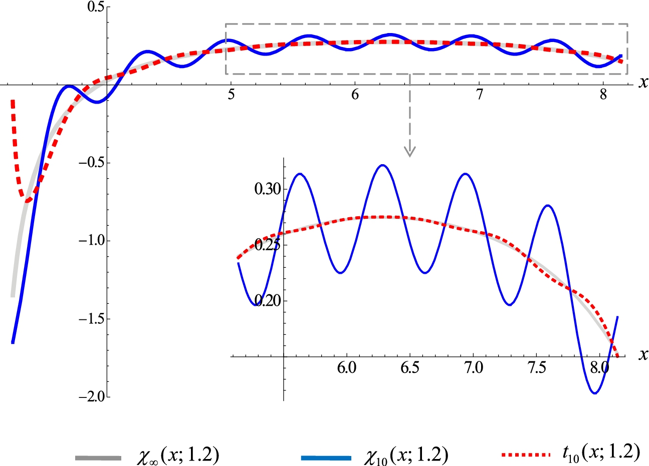
Plots of $χ_{10} (x; 1.2)$ , $χ_{\infty} (x; 1.2)$ , and $t_{10} (x; 1.2)$ as function of x. In the top figure, the leftmost point is $x = π + 0.1$ .

Fig. 5.

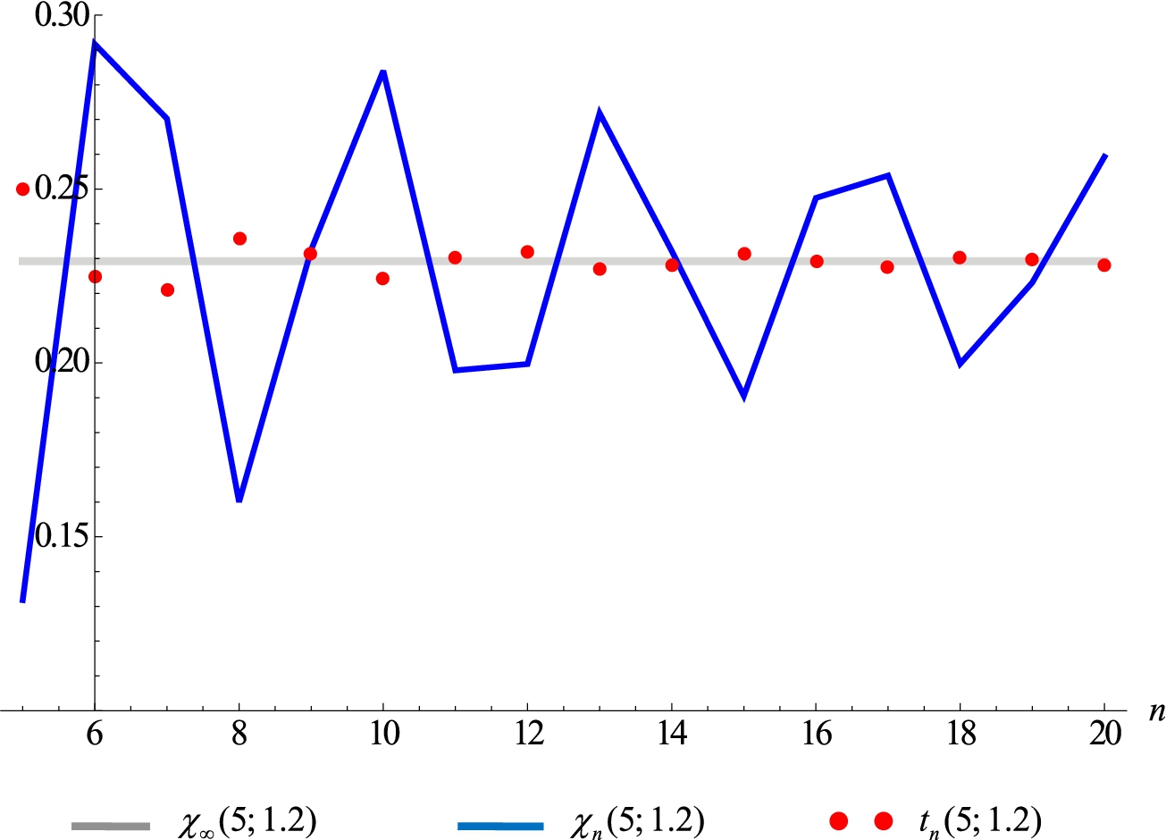
Plots of $χ_{n} (5; 1.2)$ (points joined by straight lines), $χ_{\infty} (5; 1.2)$ (horizontal solid line), and $t_{n} (5; 1.2)$ (dots) as function of n.

Our results for the three sums in Table 3 are very similar to one another. Accordingly, Fig. 4 shows representative results pertaining only to Entry 3: In Fig. 4, $n = 10$ , $λ = 1.2$ . It is seen that the original sum $χ_{10} (x; 1.2)$ oscillates about the final value $χ_{\infty} (x; 1.2)$ . Far from $x = π$ , where the singularity occurs, the transformed sum $t_{10} (x; 1.2)$ is much closer to $χ_{\infty} (x; 1.2)$ than is the original sum and much less oscillatory, having significantly reduced the Gibbs phenomenon for this logarithmic case. The best agreement occurs near $x = 2 π$ . Near $x = π$ , on the other hand, $t_{10} (x; 1.2)$ approaches infinity and differs from both $χ_{\infty} (x; 1.2)$ and $χ_{10} (x; 1.2)$ . Therefore, our CAM (64) substantially accelerates convergence, with the exception of a region very close to the logarithmic singularity (where our CAM fails, as expected from the discussions in Section 6.1). This is also evident from Fig. 5, which shows results as function of n: the values $t_{n} (5; 1.2)$ approach the final value (horizontal line) much faster than do the values $f_{n} (5; 1.2)$ .

In Figs. 4 and 5, we used not-too-large values of n ([3] uses larger values) and, to the scale shown, our results are surely free of roundoff. A comparison of (62) and (64) to other CAMs that exist in the literature is beyond the scope of this paper. Although such a comparison can be facilitated by the methods of Sections 4 and 5, CAMs are, in general, highly susceptible to roundoff and noise in the original sequence [7]. Thus, a complete comparison must also discuss issues of this nature.

7. Summary

For the trigonometric sums $c_{n} (θ)$ , $s_{n} (θ)$ , and $r_{n} (θ)$ , simple asymptotic approximations are written in Table 1 under the name “large-n (far)” formulas, where “far” means away from the point of anomaly. Table 1 also contains corresponding “large-n (near)” formulas. (Section 3.2 contains an additional term for each of the three large-n (near) formulas, not written in Table 1.) More precisely, our large-n (far) formulas hold for fixed θ, while the large-n (near) formulas hold subject to (19) or (32). Section 3.3 discusses certain relations of entries in Table 1 to formulas in the literature – note, especially, the novelty (despite its simplicity) of the $O (1)$ term in the logarithmic case. Section 3.3 further shows that the numerical accuracy obtainable from Table 1 is very high.

Table 2 is like Table 1, but for the Fejér averages of the three trigonometric sums. (It is once again possible to obtain additional terms.) By means of Tables 1 and 2, in Section 5 we discussed and graphically illustrated a number of asymptotic features of the Fejér averaging method.

This method does have certain disadvantages. Some were brought out in Section 5 (for example, the 23% difference close to the discontinuity point, and – despite the lack of strong oscillations – the unchanged order ( $O (1 / n)$ ) of the error).

The literature discusses additional disadvantages, and proposes many other methods that can better overcome the Gibbs phenomenon, examples being the Lanczos sigma factor [20,25,40], the raised cosine filter [25], and Poisson–Abel summation [39]. Based on our large-n (far) formula for the logarithmic case, we developed yet another method in Section 6. Future work will concentrate on analyzing such methods (and, if possible, comparing them amongst themselves) by the techniques of Sections 4 and 5. To do so, it is important to be able to express each transformed sum in terms of elementary functions and the original sum, as was done in Section 4.2 for the case of Fejér averaging.

Footnotes

Acknowledgement

The authors thank Professor Nikolaos L. Tsitsas for valuable remarks on the manuscript.

References

C.A.

Balanis, Antenna Theory, Analysis and Design, 3rd edn, Wiley, 2005, Section 7.4.2.

J.P.

Boyd, A lag-averaged generalization of Euler’s method for accelerating series, Appl. Math. Comput. 72 (1995), 143–166.

J.P.

Boyd, Acceleration of algebraically-converging Fourier series when the coefficients have series in powers of

1 / n

, J. Comput. Phys. 228 (2009), 1404–1411. doi:10.1016/j.jcp.2008.10.039.

J.P.

Boyd, A proof, based on the Euler sum acceleration, of the recovery of an exponential (geometric) rate of convergence for the Fourier series of a function with Gibbs phenomenon, in: Spectral and High Order Methods for Partial Differential Equations,

J.S.

Hesthave and

E.M.

Ronquist, eds, Lecture Notes in Computational Science and Engineering, Vol. 76, Springer, Berlin Heidelberg, 2011, pp. 131–139.

J.P.

Boyd, A proof, based on the Euler sum acceleration, of the recovery of an exponential (geometric) rate of convergence for the Fourier series of a function with Gibbs phenomenon, 2010, Available at: http://arxiv.org/abs/1003.5263.

Brezinski, Extrapolation algorithms for filtering series of functions, and treating the Gibbs phenomenon, Numer. Algorithms 36 (2004), 309–329. doi:10.1007/s11075-004-2843-6.

Brezinski and

Redivo Zaglia, Extrapolation Methods: Theory and Practice, Elsevier, New York, 1991.

O.P.

Bruno,

Han and

M.M.

Pohlman, Accurate, high-order representation of complex three-dimensional surfaces via Fourier continuation analysis, J. Comput. Phys. 227 (2007), 1094–1125. doi:10.1016/j.jcp.2007.08.029.

J.T.

Bushberg,

J.A.

Seibert,

E.M.

Leidholdt and

J.M.

Boone, The Essentials Physics of Medical Imaging, 2nd edn, Lippincott Williams and Wilkins, Philadelphia, 2003, chapt. 15.

10.

H.S.

Carslaw, An Introduction to the Theory of Fourier’s Series and Integrals, 3rd revised edn, Dover, New York, 1950.

11.

Dillmann and

Grabitz, On a method to evaluate Fourier–Bessel series with poor convergence properties and its application to linearized supersonic free jet flow, Quart. Appl. Math. LIII (1995), 335–352. doi:10.1090/qam/1330656.

12.

Engelburg, Edge detection using Fourier coefficients, American Mathematical Monthly 115 (2008), 499–513.

13.

Ern and

J.-L.

Guermond, Theory and Practice of Finite Elements, Springer, New York, 2004.

14.

Fikioris and

Andrianesis, Asymptotic expansions pertaining to logarithmic series and related trigonometric sums, Journal of Classical Analysis 7 (2015), 113–127. doi:10.7153/jca-07-11.

15.

Fikioris,

Tastsoglou and

O.N.

Bakas, Selected Asymptotic Methods with Applications to Electromagnetics and Antennas, Morgan and Claypool Publishers, 2013.

16.

Gottlieb and

S.A.

Orszag, Numerical Analysis of Spectral Methods: Theory and Applications, SIAM, Philadelphia, PA, 1977, Section 3.

17.

Gottlieb and

C.-W.

Shu, On the Gibbs phenomenon and its resolution, SIAM Rev. 39 (1997), 644–668. doi:10.1137/S0036144596301390.

18.

Gottlieb,

C.-W.

Shu,

Solomonoff and

Vandeven, On the Gibbs phenomenon I: Recovering exponential accuracy from the Fourier partial sum of a nonperiodic analytic function, J. Comput. Appl. Math. 43 (1992), 81–98. doi:10.1016/0377-0427(92)90260-5.

19.

Gottlieb,

J.-H.

Jung and

Kim, A review of David Gottlieb’s work on the resolution of the Gibbs phenomenon, Commun. Comput. Phys. 9 (2011), 497–519. doi:10.4208/cicp.301109.170510s.

20.

R.W.

Hamming, Numerical Methods for Scientists and Engineers, Dover, 1986.

21.

Hewitt and

R.E.

Hewitt, The Gibbs–Wilbraham phenomenon: An episode in Fourier analysis, Arch. Hist. Exact Sci. 21 (1979), 129–160. doi:10.1007/BF00330404.

22.

E.J.

Hinch, Perturbation Methods, Cambridge University Press, 1991 Section 2.5.

23.

M.Y.

Hussaini,

Kumar and

M.D.

Salas (eds), Algorithmic Trends in Computational Fluid Dynamics, Springer, New York, 1993.

24.

A.J.

Jerri, The Gibbs Phenomenon in Fourier Analysis, Splines, and Wavelet Approximations, Kluwer Academic Publishers, Dordrecht, The Netherlands, 1998.

25.

A.J.

Jerri, Advances in the Gibbs Phenomenon, Sampling Publishing, 2011.

26.

L.B.W.

Jolley, Summation of Series, Dover, 1961, p. 79 and 96.

27.

T.W.

Körner, Fourier Analysis, Cambridge University Press, Cambridge, UK, 1988, pp. 62–66. doi:10.1017/CBO9781107049949.019.

28.

B.C.

Kress and

Meyrueis, Applied Digital Optics: From Micro-Optics to Nanophotonics, Wiley, New York, 2009.

29.

Lanczos, Discourse on Fourier Series, Oliver & Boyd, London, 1966.

30.

J.N.

Libii, Gibbs phenomenon and its applications in science and engineering, in: Proceedings of the 2005 American Society for Engineering Education Annual Conference & Exposition, 2005, pp. 10.666.1–10.666.12. Available at: https://peer.asee.org/gibbs-phenomenon-in-engineering-systems.pdf.

31.

Oberhettinger, Fourier Expansions: A Collection of Formulas, Academic Press, New York, 1973.

32.

Oleksy, A convergence acceleration method of Fourier series, Comput. Phys. Commun. 96 (1996), 17–26. doi:10.1016/0010-4655(96)00044-6.

33.

F.W.J.

Olver,

D.W.

Lozier,

R.F.

Boisvert and

C.W.

Clark (eds), NIST Handbook of Mathematical Functions, Cambridge University Press, Cambridge, 2010.

34.

J.G.

Proakis and

D.G.

Manolakis, Digital Signal Processing, 3rd edn, Prentice-Hall, New Jersey, 1996, chapt. 8.

35.

A.P.

Prudnikov,

Y.A.

Brychkov and

O.I.

Marichev, Integrals and Series., Vol. 1, Elementary Functions, Gordon and Breach, London, UK, 1986.

36.

W.A.

Strauss, Partial Differential Equations, 2nd edn, Wiley, New York, 2008, pp. 142–144.

37.

Strichartz, Gibbs’ phenomenon and arclength, The Journal of Fourier Analysis 6 (2000), 533–536. doi:10.1007/BF02511544.

38.

N.M.

Temme, Special Functions – an Introduction to the Classical Functions of the Mathematical Physics, Wiley, 1996.

39.

Vretblad, Fourier Analysis and Its Applications, Springer, New York, 2003, pp. 93–96. doi:10.1007/b97452.

40.

E.W.

Weisstein, Gibbs Phenomenon. From MathWorld – A Wolfram Web Resource, Available at http://mathworld.wolfram.com/GibbsPhenomenon.html.

41.

Wong, Asymptotic Approximations of Integrals, SIAM, Philadelphia, 2001. doi:10.1137/1.9780898719260.

42.

Zygmund, Trigonometric Series, 2nd edn, Cambridge University Press, 1968.

Asymptotic approximations elucidating the Gibbs phenomenon and Fejér averaging

Abstract

Keywords

1. Introduction

3. Asymptotic approximations for c n ( θ ) , s n ( θ ) , and r n ( θ )

3.1. Large-n (far) formulas

3.3. Comparisons with formulas in the literature; initial numerical results

4.1. Definitions

4.2. Derivations

5.1. Fejér averaging eliminates dominant oscillations, but preserves the order of the error

5.2. “Asymptotic intersection points” of Fejér averages

5.3. Values of Fejér averages at first overshoot and undershoot

5.4. Numerical illustrations of asymptotic predictions

6.1. CAM for c n ( θ )

6.2. Applicability of the CAM to other sums; test cases

Footnotes

Acknowledgement

References

3. Asymptotic approximations for $c_{n} (θ)$ , $s_{n} (θ)$ , and $r_{n} (θ)$

6.1. CAM for $c_{n} (θ)$