Spectral analysis of a non-selfadjoint operator generated by an energy harvesting model and application to an exact controllability problem

Abstract

The present paper is the second one in a series of three works dealing with a mathematical model for an electro-mechanical energy harvester. The harvester is designed as a beam with a piezoceramic layer attached to its top face. A pair of conductive electrodes, covering the top and bottom faces of the piezoceramic layer, are connected to a resistive load. The model is governed by a system of two differential equations. The first of them is the equation of the Euler–Bernoulli beam model subject to actions of an external damping and of an external force. The second equation represents the Kirchhoff’s law for the electric circuit. Both equations are coupled by means of the direct and converse piezoelectric effects. The system is represented as a single operator evolution equation in a Hilbert space (the state space). The dynamics generator of this system is a non-selfadjoint operator with a compact resolvent. In the first paper, the asymptotic formulas for the eigenvalues of the dynamics generator have been derived. In the present paper, the following results have been shown. 1) The set of the generalized eigenvectors of the dynamics generator is complete and minimal in the state space. 2) The set of normalized generalized eigenvectors forms a Riesz basis, which is quadratically close to an orthonormal basis (a Bari basis). 3) The exact controllability problem has been solved via the spectral decomposition method.

Keywords

Electro-mechanical energy harvester non-selfadjoint matrix differential operator generalized eigenvectors Bari basis exact and approximate controllability

1. Introduction

The present paper is the second part of the three-part set of papers devoted to the asymptotic, spectral, and controllability results for a certain class of energy harvesting models. The models are widely accepted in modern engineering literature and a lot of experimental data is available. However, rigorous mathematical analysis is mostly an open research area (see [5,6] and references therein). In our sequence of papers, we consider the model of a piezoelectric energy harvester, which is designed as a beam with a piezoceramic layer attached to its top face (unimorph configuration). The model is governed by a system of two equations, the first of which is the equation of the Euler–Bernoulli model for the transverse vibrations of the beam and the second one represents the Kirchhoff’s law for the electric circuit and describes the voltage dynamics on the surface of the piezoceramic layer. Both equations are coupled due to the direct and converse piezoelectric effects; to keep sustainable vibrational motion the external forcing is used. The boundary conditions describe the structure clamped at the left end and free at the right one. We represent the system as a single operator evolution equation in a Hilbert space. The dynamics generator of this system is a non-selfadjoint operator with compact resolvent. Our main results in the first paper of the series [20] include formulas for the inverse and the adjoint operators and an explicit asymptotic formula for the eigenvalues of this generator, i.e., we perform the modal analysis for electrically loaded (not short-circuit) system. We show that the spectrum splits into an infinite sequence of stable eigenvalues that approach a vertical line in the left half plane and possibly of a finite number of unstable eigenvalues. In the present paper we focus on geometric properties of the set of the generalized eigenvectors of the model, i.e., we show that this set is complete and minimal in the state space and forms an unconditional basis, which is quadratically close to an orthonormal basis (the Bari basis). We also present the application of the spectral and asymptotic results to an exact controllability problem which we solve via the spectral decomposition method. Before presenting our mathematical results, we would like to give a brief description of the model (see [5,6,20] for details).

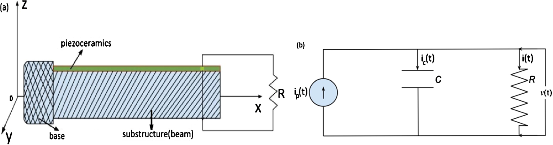
Description of the model. The following sketch Fig. 1(a) shows the construction of the harvester. The electrical circuit of the harvester is presented on Fig. 1(b).

Fig. 1.

Unimorph cantilever with a piezoceramic layer connected to a resistive load.

We consider a piezoelectric energy harvester in the form of a thin cantilever (clamped-free) beam with a piezoceramic layer. We use the Euler–Bernoulli model to describe the transverse vibrations of the beam. The piezoceramic layer is attached to the top face of the beam; a pair of electrodes is covering the top and the bottom faces of the piezoceramic layer. The thickness of the electrodes can be neglected and they are perfectly conductive. The electrodes are connected to a resistive load. The load is considered in an electrical circuit along with the internal capacitance of the piezoceramic layer, which is assumed to be a perfect insulator. If the beam vibrates due to some external load, then a dynamic strain appears in the piezoceramic layer. Due to the piezoelectric effect this strain results in an alternating voltage output across the electrodes. This output can be harvested for charging batteries or running low-powered electronic devices [5,6].

On the other hand, the electric potential difference between the electrodes generates an electric field in the piezoceramic layer [5,6,20]. This electric field produces a stress on the piezoceramic due to the converse piezoelectric effect. So, the dynamics of the beam is affected by the electric circuit. As a result, the energy harvester is modeled by a coupled system of two differential equations. The first of them is an equation for the Euler–Bernoulli beam that contains an additional term depending on the voltage on the electrodes (see Eq. (1.1) below). This term represents the converse piezoelectric effect. In other words the backward piezoelectric coupling effect affects the vibration response of the cantilever. The second equation is just the Kirchhoff’s law for the electric circuit. This equation is a linear first order differential equation with respect to the voltage across the electrodes. The equation contains an additional integral term depending on the transverse displacement of the beam (see Eq. (1.2) below). This term represents the direct piezoelectric effect.

The paper is organized as follows. In the remaining part of Section 1 we provide the formulation of the initial boundary-value problem in the form borrowed from the engineering literature (see, e.g., monograph [6] and references therein). Using a variational approach we reformulate the problem in a way convenient for mathematical treatment.

In Section 2 the operator setting of the model in the appropriate state space is given and the main object of interest, the system dynamics generator, is identified. We reproduce the main result of paper [20], i.e., the asymptotics of the eigenvalues of the dynamics generator, when the number of an eigenvalue tends to infinity (Theorem 3.2 below). The spectral asymptotics are needed for derivation of the results of Sections 4–6.

Section 3 deals with reduction of the spectral problem for a matrix differential operator (the dynamics generator) to the eigenvalue-eigenfunction problem for a corresponding non-selfadjoint quadratic operator pencil (see formulas (3.5) and (3.6) below). It is a non-standard pencil since the spectral parameter enters the description of the pencil’s domain. Having an eigenfunction of the pencil, one can easily construct a three-component eigenvector of the dynamics generator, $L$ .

Section 4 is concerned with the completeness of the generalized eigenvectors (the eigenvectors and associate vectors together) in the state Hilbert space. To prove the completeness property, one has to obtain specific estimates on the rate of growth of the resolvent of $L$ . Had we have the fact that the operator $L$ is dissipative, we could have used the results of paper [18], where application of M.G. Krein’s Theorem yields completeness result without heavy calculations. However, in the present paper, $L$ is not a dissipative operator, which implies derivation of quite complicated formulas in order to prove the desired estimates on the resolvent of $L$ .

In Section 5 the proof of the Bari-basis property of the generalized eigenvectors is presented. The main tool in the proof is establishing the fact that the sets of the generalized eigenvectors of the operators $L$ and $L^{*}$ are quadratically closed (see Theorem 5.1 below).

Section 6 deals with solving the exact and approximate controllability problems via the spectral decomposition method [1,17]. We present explicit formulas for the control laws in terms of the set of non-harmonic exponentials and the set which is biorthogonal to the above set of the exponentials. To solve the control problems we need both the Riesz basis property of the generalized eigenvectors of the operator $L$ and the Riesz basis property of the set of non-harmonic exponentials built on the eigenvalues of the operator $L$ .

In the conclusion of the Introduction, we mention that the methods of asymptotic and spectral analysis are proven to be very efficient in many areas of the applied sciences such as fluid-structure interactions [14], vibrational mechanics [3], aeroelasticity [2,4], and applied solid mechanics [9].

Statement of the initial boundary-value problem. We consider a system of two coupled differential equations for two unknown functions $w (x, t)$ and $v (t)$ with $0 ⩽ x ⩽ L < \infty$ , $t ⩾ 0$ (see [5,6]). In what follows, we use the subindex notations for partial derivatives. $\begin{array}{l} (1.1) & m w_{t t} + c_{a} w_{t} + Y I w_{x x x x} (x, t) - θ ν (t) [δ^{'} (x) - δ^{'} (x - L)] = 0, \\ (1.2) & C v_{t} (t) + \frac{1}{R} v (t) + κ \int_{0}^{L} w_{x x t} (x, t) d x = 0 . \end{array}$ This system is equipped with the following set of the boundary conditions: $\begin{matrix} (1.3) & w (0, t) = w_{x} (0, t) = 0, Y I w_{x x} (L, t) = 0, Y I w_{x x x} (L, t) = 0 . \end{matrix}$ Here $w (x, t)$ – the transverse displacement of the beam at a position x at time moment t; m – mass per unit length; $c_{a}$ – viscous air damping coefficient; Y – the Young modulus; I – cross section moment of inertia with respect to the neutral axis ( $Y I$ – the bending stiffness); θ – converse piezoelectric effect backward coupling coefficient; $v (t)$ – the output voltage across the electrodes of the piezoceramic layer; C – internal capacitance of the piezoceramic layer; R – resistance of the external load; κ – direct piezoelectric effect coupling coefficient; δ – Dirac’s delta-function. The first and third terms in (1.1) represent an undamped beam.

Using a variational approach in [20], it has been shown that problem (1.1)–(1.3) is equivalent to the following initial boundary-value problem: $\begin{array}{l} (1.4) & m w_{t t} (x, t) + c_{a} w_{t} (x, t) + Y I w_{x x x x} (x, t) = 0, \\ (1.5) & C v_{t} (t) + \frac{1}{R} v (t) + κ [w_{t x} (L, t) - w_{t x} (0, t)] = 0 . \end{array}$ System (1.4) and (1.5) is equipped with boundary conditions (1.3) and standard initial conditions $\begin{matrix} (1.6) & w (x, 0) = w_{0} (x), w_{t} (x, 0) = w_{1} (x), v (0) = v_{0} . \end{matrix}$

2. Operator reformulation of the problem

It is convenient to use scaled physical quantities with the new set of notations. Let $\begin{matrix} (2.1) & G = \frac{c_{a}}{m}, E = \frac{Y I}{m}, H = \frac{1}{C R}, h = \frac{κ}{C}, Θ = \frac{θ}{m} . \end{matrix}$ Equations (1.4), (1.5) in new notation have the form $\begin{matrix} (2.2) & \begin{matrix} w_{t t} (x, t) + G w_{t} (x, t) + E w_{x x x x} (x, t) = 0, \\ v_{t} (t) + H v (t) + h [w_{t x} (L, t) - w_{t x} (0, t)] = 0 . \end{matrix} \end{matrix}$ The boundary conditions become $\begin{matrix} (2.3) & w (0, t) = w_{x} (0, t) = 0, E w_{x x} (L, t) = Θ v (t), w_{x x x} (L, t) = 0 . \end{matrix}$ Our goal is to rewrite the problem (2.2) and (2.3) as an operator evolution equation in the state space of the system, which is a Hilbert space of the Cauchy data equipped with the energy norm. First we accomplish some preliminary steps.

Let $w (x, t)$ and $v (t)$ be a solution set of the above system. Let us introduce a vector of solution $U (x, t) = {(w (x, t), w_{t} (x, t), v (t))}^{T}$ and fix $t > 0$ . Consider a three-component vector-function of x. (Without misunderstanding we use the same notation U.) $\begin{matrix} (2.4) & U (x) = {(u_{0} (x), u_{1} (x), u_{2})}^{T} . \end{matrix}$

Definition 2.1.
Energy space $H = H_{0}^{2} (0, L) \times L^{2} (0, L) \times C$ is the closure of smooth functions satisfying conditions $u_{0} (0) = u_{0}^{'} (0) = 0$ in the norm $\begin{matrix} (2.5) & ‖ U ‖_{H}^{2} = \frac{1}{2} [\int_{0}^{L} (E {| u_{0}^{″} (x) |}^{2} + {| u_{1} (x) |}^{2}) d x + | u_{2} |^{2}] . \end{matrix}$ It is convenient to keep the notation $H_{0}^{2} (0, L)$ for the set of functions satisfying the boundary conditions only at the left end. However, this is a slight abuse of standard notation when an element from $H_{0}^{2} (0, L)$ satisfies the same boundary conditions at both ends. It can be directly verified that system (2.2), (2.3), and (1.6) can be given in the form of an evolution equation $\begin{matrix} (2.6) & \frac{d}{d t} U (x, t) = i (L U) (x, t) . \end{matrix}$ The dynamics generator, the main object of interest, is a matrix differential operator given by the differential expression $\begin{matrix} (2.7) & L = - i [\begin{matrix} 0 & 1 & 0 \\ - E \frac{d^{4}}{d x^{4}} & - G & 0 \\ 0 & - h A_{L} & - H \end{matrix}], \end{matrix}$ with $A_{a}$ being the differential operation defined on a smooth function $f (x)$ by $\begin{matrix} (2.8) & A_{a} [f] = f^{'} (a), \end{matrix}$ and $L$ being defined on the domain $\begin{array}{rcl} D (L) & = & {U = {(u_{0}, u_{1}, u_{2})}^{T} \in H : u_{0} \in H^{4} (0, L) \cap H_{0}^{2} (0, L), \\ (2.9) & u_{1} \in H_{0}^{2} (0, L), u_{2} \in C; u_{0}^{‴} (L) = 0, E u_{0}^{″} (L) = Θ u_{2}} . \end{array}$

The adjoint operator. Recall [8] that the adjoint operator $L^{}$ satisfies $\begin{matrix} {(L U, V)}_{H} = {(U, L^{} V)}_{H} for any U \in D (L), V \in D (L^{}) . \end{matrix}$

The operator $L^{}$ adjoint to $L$ is given by the following differential expression $\begin{matrix} (2.10) & L^{} = - i [\begin{matrix} 0 & 1 & 0 \\ - E \frac{d^{4}}{d x^{4}} & G & 0 \\ 0 & - Θ A_{L} & H \end{matrix}], \end{matrix}$ defined on the domain $\begin{array}{rcl} D (L^{}) & = & {V \in H : v_{0} \in H^{4} (0, L) \cap H_{0}^{2} (0, L), v_{1} \in H_{0}^{2} (0, L), \\ (2.11) & v_{1} (0) = v_{1}^{'} (0) = v_{0}^{‴} (L) = 0; E v_{0}^{″} (L) = h v_{2}} . \end{array}$
Remark 2.2.
Notice, there are two reasons for the non-selfadjointness of the operator $L$ . Namely, the differential expressions (2.7) and (2.10) are different as well as the domains (2.9) and (2.11) are different as well.

Now we present the main spectral result of paper [20]. Theorem 2.3.

Operator $L$ is a non-selfadjoint matrix differential operator in $H$ , whose resolvent is a compact operator. The spectrum of $L$ is discrete with the only accumulation point at infinity; each eigenvalue is normal, i.e. it is an isolated point of spectrum of a finite algebraic multiplicity.

The spectrum located in the lower half-plane of the complex plane is finite; the number of real eigenvalues is at most finite. The spectrum is symmetric with respect to the imaginary axis, i.e., $λ_{- n} = - {\overline{λ}}_{n}$ , $n = 1, 2, 3, \dots$ .

The following asymptotic approximation is valid for the eigenvalues as the number of an eigenvalue tends to infinity: $\begin{matrix} (2.12) & λ_{n} = \sqrt{E} {(\frac{π}{L})}^{2} (n^{2} + n) + [{(\frac{π}{2 L})}^{2} + \frac{2 Θ h}{L}] + i \frac{G}{2} + O (\frac{1}{n}), n \to \infty, λ_{- n} = - {\overline{λ}}_{n} . \end{matrix}$

In general, the operator $L$ is not a dissipative operator unless $Θ = h$ .

There may exist only a finite number of the eigenvalues whose algebraic multiplicity is greater than 1; the geometric multiplicity of any eigenvalue is 1. Hence there may be only a finite number of the associate vectors.

Remark 2.4.
As stated in the above theorem, $L$ is a dissipative operator only when $Θ = h$ . (We recall that a linear operator A in a Hilbert space H is dissipative if $ℑ {(A f, f)}_{H} ⩾ 0$ for any $f \in D (A)$ (see, e.g., [8,12,13]).) As we know, the parameter $h = κ / C$ with κ being a direct piezoelectric effect coefficient and C being an internal piezoelectric layer capacitance, and the parameter $Θ = θ / m$ with θ being an inverse piezoelectric effect coefficient and m being the density of structure. However, in practical ranges of the physical parameters Θ and h are quite different numerically, which means that we are dealing with non-selfadjoint (and non-dissipative) operators. This observation is important in our proof of completeness of the generalized eigenfunctions of $L$ in $H$ . Namely, if the operator $L^{- 1}$ is a dissipative one, than to prove completeness, we can use the results of paper [18] and apply the corresponding results of the operator $L^{- 1}$ . However, if we do not have a dissipativity property, we have no choice but to use the general approach which is concerned with the estimates on the norm of the resolvent operator $R_{λ} [L] = {(L - λ I)}^{- 1}$ on a specific set of rays on the complex plane $λ \in C$ as $| λ | \to \infty$ .

3. The spectral equation

In paper [20], we have derived the equation whose solutions are the eigenvalues of the operator $L$ . In what follows we need an explicit representation for the eigenvectors of $L$ . For reader’s convenience we reproduce the main formulas from [20] that yield the explicit formulas for the eigenvectors of the polynomial pencil $P (\cdot)$ associated to the operator $L$ . To this end, we have reduced the spectral problem for the operator $L$ to the spectral problem for the corresponding polynomial pencil $P (\cdot)$ . Knowing formula for an eigenfunction of the pencil, one can readily reconstruct explicit formula for the corresponding three-component eigenvector of $L$ . The eigenvalue-eigenvector equation, $L U = λ U$ , for $U = {(u_{0}, u_{1}, u_{2})}^{T} \in D (L)$ generates the following system for the components of U: $\begin{matrix} (3.1) & u_{1} (x) = i λ u_{0} (x), E u_{0}^{''''} (x) + G u_{1} (x) = - i λ u_{1} (x), h u_{1}^{'} (L) + H u_{2} = - i λ u_{2} . \end{matrix}$ Eliminating $u_{1}$ from this system and taking into account that $u_{2} = Θ^{- 1} E u_{0}^{″} (L)$ yields the spectral problem, $P (λ) φ = 0$ , for a quadratic operator pencil $P (\cdot)$ (see [12]) defined by the formula $\begin{matrix} (3.2) & P (λ) φ = E φ^{''''} + i λ G φ - λ^{2} φ \end{matrix}$ on the domain $\begin{array}{rcl} D (P) & = & {φ \in H^{4} (0, L) : φ (0) = φ^{'} (0) = φ^{''''} (0) = 0, \\ (3.3) & Θ^{- 1} E (H + i λ) φ^{″} (L) + i λ h φ^{'} (L) = 0} . \end{array}$ Notice, $P (\cdot)$ is a non-standard pencil since the spectral parameter λ enters the domain explicitly. This type of pencils have not been considered in monograph [12]. However, it is convenient to keep the terminology because there exists an extensive literature, in which the pencils with the spectral parameter-dependent boundary conditions appear naturally. A non-trivial solution $φ \in D (P)$ of the pencil equation $P (λ) φ = 0$ will be called an eigenfunction of the pencil and the corresponding value of λ will be called an eigenvalue. The spectra of the operator $L$ and the pencil $P (\cdot)$ coincide. It is clear that having an eigenfunction of the pencil and using (3.1), we can find all components of the eigenvector of $L$ .

To solve the pencil spectral equation one has to construct the solution $φ (λ, x)$ of the equation $\begin{matrix} (3.4) & E φ^{''''} (λ, x) + i λ G φ (λ, x) - λ^{2} φ (λ, x) = 0 \end{matrix}$ satisfying boundary conditions from (3.3). Introducing new scaled parameters $\begin{matrix} (3.5) & \tilde{λ} = \frac{λ}{\sqrt{E}}, \tilde{G} = \frac{G}{\sqrt{E}}, \tilde{H} = \frac{H}{\sqrt{E}}, \tilde{Θ} = \frac{Θ h}{\sqrt{E}}, \end{matrix}$ we obtain the following Sturm–Liouville eigenvalue problem: $\begin{matrix} (3.6) & \begin{matrix} φ^{''''} (λ, x) + i \tilde{λ} \tilde{G} φ (λ, x) - {(\tilde{λ})}^{2} φ (λ, x) = 0, \\ φ (λ, 0) = φ^{'} (λ, 0) = φ^{‴} (L) = 0, (\tilde{H} + i \tilde{λ}) φ^{″} (λ, L) + i \tilde{λ} \tilde{Θ} φ^{'} (λ, L) = 0 . \end{matrix} \end{matrix}$ Omitting “tilde” from problem (3.6), we consider the rescaled problem: $\begin{array}{l} (3.7) & φ^{''''} (λ, x) - λ^{2} φ (λ, x) + i λ G φ (λ, x) = 0, \\ (3.8) & φ (λ, 0) = φ^{'} (λ, 0) = 0, φ (λ, L) = 0, (H + i λ) φ^{″} (λ, L) + i λ Θ φ^{'} (λ, L) = 0 . \end{array}$ The solution satisfying three conditions $φ (λ, 0) = φ^{'} (λ, 0) = φ (λ, L) = 0$ can be given in the form [13] $\begin{array}{rcl} φ (λ, x) & = & [cosh (μ (λ) L) + cos (μ (λ) L)] [cosh (μ (λ) x) - cos (μ (λ) x)] \\ (3.9) & - [sinh (μ (λ) L) - sin (μ (λ) L)] [sinh (μ (λ) x) - sin (μ (λ) x)], \end{array}$ where $μ (λ)$ is defined as follows: $\begin{matrix} (3.10) & μ (λ) = \sqrt[4]{λ^{2} - i λ G} = \sqrt{λ} - \frac{i G}{4 \sqrt{λ}} + \frac{3 G^{2}}{2^{5} λ^{3 / 2}} + O (\frac{1}{λ^{5 / 2}}), | λ | \to \infty, \end{matrix}$ and the branch of $\sqrt[4]{z}$ is fixed by the conditions $ℜ \sqrt[4]{z} > 0$ and $ℑ \sqrt[4]{z} ⩾ 0$ for $ℑ z ⩾ 0$ . The fourth boundary condition from (3.8) generates the following spectral equation: $\begin{array}{l} μ (λ) (H + i λ) [1 + cosh (μ (λ) L) cos (μ (λ) L)] \\ (3.11) & + i λ Θ [cosh (μ (λ) L) sin (μ (λ) L) + sinh (μ (λ) L) cos (μ (λ) L)] = 0 . \end{array}$ The asymptotic distribution of the roots of Eq. (3.11) (and thus the asymptotics of the eigenvalues of $L$ ) is given in Theorem 2.3 above. (In that theorem (see (2.12)) we have used the parameters introduced in (2.1) but not the parameters introduced in (3.5).)

To proceed with the proof of completeness and minimality of the set of the generalized eigenvectors, we recall several definitions.

Definition 3.1.

A set of vectors ${φ_{n}}_{n \in Z^{'}}$ in a Hilbert space H is almost normalized if there exist two positive constants $C_{1}$ and $C_{2}$ such that $\begin{matrix} (3.12) & 0 < C_{1} ⩽ ‖ φ_{n} ‖_{H} ⩽ C_{2} < \infty, n \in Z^{'}, Z^{'} = Z ∖ {0} . \end{matrix}$

Two sets of vectors ${φ_{n}}_{n \in Z^{'}}$ and ${ψ_{n}}_{n \in Z^{'}}$ are biorthogonal if the following relations hold: $\begin{matrix} (3.13) & {(φ_{n}, ψ_{m})}_{H} = δ_{n m}, m, n \in Z^{'} . \end{matrix}$

A set of vectors ${φ_{n}}_{n \in Z^{'}}$ in a Hilbert space H forms a Riesz basis if this set is a linear isomorphic image of an orthonormal basis ${φ_{n}^{0}}_{n \in Z^{'}}$ (i.e., a Riesz basis is an almost normalized unconditional basis).

A Riesz basis ${φ_{n}}_{n \in Z^{'}}$ which is quadratically close to an orthonormal basis ${φ_{n}^{0}}_{n \in Z^{'}}$ , i.e., $\sum_{n \in Z^{'}} ‖ φ_{n} - φ_{n}^{0} ‖_{H}^{2} < \infty$ , is called a Bari basis.

One of the main results of the present paper is the following statement.
Theorem 3.2.
The set of the generalized eigenvectors of the operator $L$ forms a Bari basis in $H$ . The set of the generalized eigenvectors of the adjoint operator $L^{}$ forms a biorthogonal Bari basis in* $H$ .

The main tool in proving Theorem 3.2 is the following Bari’s Theorem.
Theorem 3.3 ([8, p. 389]).

For a complete, almost normalized sequence of vectors ${φ_{n}}_{n \in Z^{'}}$ to form a Bari basis in $H$ , it is necessary and sufficient that there exists a sequence ${ψ_{n}}_{n \in Z^{'}}$ , biorthogonal to ${φ_{n}}_{n \in Z^{'}}$ , and that both sequences are quadratically close, i.e., $\begin{matrix} (3.14) & \sum_{n \in Z^{'}} ‖ φ_{n} - ψ_{n} ‖_{H}^{2} < \infty . \end{matrix}$

To make use of Bari’s Theorem, one has to show that (i) the set of the generalized eigenvectors is complete in $H$ (i.e., finite linear combinations of the generalized eigenvectors are dense in $H$ ) and (ii) the set of the generalized eigenvectors is minimal in $H$ (i.e., neither generalized eigenvector belongs to the closed linear span of the remaining vectors).

4. Completeness and minimality of the set of generalized eigenvectors

As was already mentioned, since $L$ is not a dissipative operator in general, to prove the completeness result, we will derive the estimate on the norm of the resolvent operator $R_{λ} (L) = {(L - λ I)}^{- 1}$ on a specific set of rays initiating at the origin ( $λ = 0$ ) on the complex λ-plane.

Our main tool in the proof is Theorem 6.2 from [11, p. 80]. To formulate this theorem, we recall [11, p. 78] that a densely defined closed linear operator $T$ in a separable complex Hilbert space H is called a Hilbert–Schmidt discrete operator if there is a point α in the resolvent set $ρ (T)$ such that the resolvent $R_{α} (T)$ is a Hilbert–Schmidt operator in H. Since the resolvent of the operator $L$ belongs to the class of Hilbert–Schmidt compact operators [8], we can use the following result from [11].

Theorem 4.1 ([11, p. 80]).

Let H be a separable Hilbert space. Let $T$ be a Hilbert–Schmidt discrete linear operator in H, and let $S (T) = {λ_{i}}_{i = 1}^{\infty}$ be any enumeration of the spectrum of $T$ . Assume that there exists a set of five rays $γ_{j}$ : $arg λ = θ_{j}$ , $j = 1, \dots, 5$ , in the complex plane such that (i) the angles between adjoint rays are less then $π / 2$ , (ii) for $| λ |$ sufficiently large, all the points on the five rays belong to the resolvent set $ρ (T)$ and (iii) there exists a positive integer N such that $\begin{matrix} (4.1) & ‖ R_{λ} (T) ‖ = O (| λ |^{N}) as λ \to \infty \end{matrix}$ along each ray $γ_{j}$ . Then the set of the generalized eigenvectors of $T$ is complete in H.

To derive the necessary estimates on the resolvent of the operator $L$ , we consider the following equation: $\begin{matrix} (4.2) & L F - λ F = G, G = {(g_{0}, g_{1}, g_{2})}^{T} \in H . \end{matrix}$ We derive an explicit representation for the solution of (4.2) that satisfies the boundary conditions in such a way that $F = {(f_{0}, f_{1}, f_{2})}^{T} \in D (L)$ . Equation (4.2) is equivalent to the following system: $\begin{array}{l} (4.3) & - i λ f_{0} (x) + f_{1} (x) = i g_{0} (x), \\ (4.4) & - E f_{0}^{''''} (x) - (G + i λ) f_{1} (x) = i g_{1} (x), \\ (4.5) & - h [f_{1}^{'} (L) - f_{1}^{'} (0)] - (H + i λ) f_{2} = i g_{2} . \end{array}$ Since we look for a solution $F \in H$ , we have that $f_{0} (0) = f_{0}^{'} (0) = 0$ and due to (4.3), $f_{1} \in H_{0}^{2} (0, L)$ .

Eliminating $f_{1}$ from Eq. (4.4) and using a new notation $\begin{matrix} (4.6) & g_{3} (λ, x) = - i (g_{1} (x) + g_{0} (x) (G + i λ)), \end{matrix}$ we rewrite Eq. (4.4) in the form $\begin{matrix} (4.7) & E f_{0}^{''''} (x) - λ^{2} f_{0} (x) + i λ G f_{0} (x) = g_{3} (λ, x) . \end{matrix}$ Eliminating $f_{1}$ from Eq. (4.5) and taking into account the end condition $E f_{0}^{″} (L) = Θ f_{2}$ yields $\begin{array}{l} E (H + i λ) f_{0}^{″} (L) & = Θ [- i λ h f_{0}^{'} (L) - i (g_{2} + h g_{0}^{'} (L))] \\ (4.8) & = - i λ h Θ f_{0}^{'} (L) - i Θ (g_{2} + h g_{0}^{'} (L)) . \end{array}$ Denoting $\begin{matrix} (4.9) & g_{4} = - i Θ (g_{2} + h g_{0}^{'} (L)), \end{matrix}$ we reduce (4.8) to the following boundary condition: $\begin{matrix} (4.10) & E (H + i λ) f_{0}^{″} (L) + i λ h Θ f_{0}^{'} (L) = g_{4} . \end{matrix}$ Collecting together Eq. (4.7) and all boundary conditions, we obtain that the component $f_{0}$ has to satisfy the following Sturm–Liouville eigenvalue problem: $\begin{array}{l} E φ^{''''} (λ, x) - λ^{2} φ (λ, x) + i λ G φ (λ, x) = g_{3} (λ, x), \\ (4.11) & φ (λ, 0) = φ^{'} (λ, 0) = φ^{‴} (λ, L) = 0, \\ φ^{″} (λ, L) E (H + i λ) + i λ h Θ φ^{'} (λ, L) = g_{4} . \end{array}$ Let us divide the first and third equations of (4.11) by E and introduce a new set of parameters: $\begin{matrix} \tilde{λ} = \frac{λ}{\sqrt{E}}, \tilde{G} = \frac{G}{\sqrt{E}}, {\tilde{g}}_{3} = \frac{g_{3}}{E}, \tilde{h} = \frac{h}{\sqrt{E}}, {\tilde{g}}_{4} = \frac{g_{4}}{E} . \end{matrix}$ Rewriting system (4.11) in these parameters and omitting the “tilde”, we obtain $\begin{array}{l} (4.12) & φ^{''''} (λ, x) - λ^{2} φ (λ, x) + i λ G φ (λ, x) = g_{3} (λ, x), \\ (4.13) & φ (λ, 0) = φ^{'} (λ, 0) = φ^{‴} (λ, L) = 0, \\ (4.14) & φ^{″} (λ, L) (H + i λ) + i λ h Θ φ^{'} (λ, L) = g_{4} . \end{array}$ We need an explicit formula for the solution of (4.12)–(4.14). We start with construction of the general solution of Eq. (4.12) denoted by $φ_{g} (λ, x)$ , which is a sum of the general solution of the homogeneous equation, $φ_{g}^{0} (λ, x)$ , and a particular solution of the nonhomogeneous equation $φ_{p} (λ, x)$ .

Lemma 4.2.
Equation ( 4.12 ) has a particular solution that satisfies the boundary conditions: $\begin{array}{rcl} (4.15) & \begin{matrix} a) & φ_{p} (λ, 0) = - \frac{1}{2 μ^{3} (λ)} \int_{0}^{L} [\frac{cosh (μ (λ) (L - ξ))}{sinh (μ (λ) L)} + \frac{cos (μ (λ) (L - ξ))}{sin (μ (λ) L)}] g_{3} (λ, ξ) d ξ, \\ b) & φ_{p} (λ, L) = - \frac{1}{2 μ^{3} (λ)} \int_{0}^{L} [\frac{cosh (μ (λ) ξ)}{sinh (μ (λ) L)} + \frac{cos (μ (λ) ξ)}{sin (μ (λ) L)}] g_{3} (λ, ξ) d ξ, \\ c) & φ_{p}^{″} (λ, L) = - \frac{1}{2 μ (λ)} \int_{0}^{L} [\frac{cosh (μ (λ) ξ)}{sinh (μ (λ) L)} - \frac{cos (μ (λ) ξ)}{sin (μ (λ) L)}] g_{3} (λ, ξ) d ξ, \\ d) & φ_{p}^{'} (λ, 0) = 0, φ_{p}^{'} (λ, L) = 0, φ_{p}^{‴} (λ, L) = 0, \end{matrix} \end{array}$ where $μ (λ)$ is defined in ( 3.10 ). This particular solution is given by the following formula: $\begin{array}{rcl} φ_{p} (λ, x) & = & - \frac{1}{2 μ^{3} (λ)} {\int_{x}^{L} [\frac{cosh (μ (λ) x) cosh (μ (λ) (L - ξ))}{sinh (μ (λ) L)} \\ + \frac{cos (μ (λ) x) cos (μ (λ) (L - ξ))}{sin (μ (λ) L)}] g_{3} (λ, ξ) d ξ \\ - \int_{0}^{x} [\frac{cosh (μ (λ) ξ) cosh (μ (λ) (L - x))}{sinh (μ (λ) L)} \\ (4.16) & + \frac{cos (μ (λ) ξ) cos (μ (λ) (L - x))}{sin (μ (λ) L)}] g_{3} (λ, ξ) d ξ} . \end{array}$
Proof.
To find the particular solution, we use the method of variation of parameters [13,23], i.e., we look for this solution in the form $\begin{matrix} (4.17) & φ_{p} (λ, x) = - \sum_{j = 1}^{4} C_{j} (λ, x) ψ_{j} (λ, x), \end{matrix}$ where ${ψ_{j}}_{j = 1}^{4}$ is the fundamental system of solutions of Eq. (4.12) when $g_{3} (λ, x) = 0$ , i.e., $\begin{matrix} (4.18) & \begin{matrix} ψ_{1} (λ, x) = cosh (μ (λ) x), ψ_{2} (λ, x) = cosh (μ (λ) (L - x)), \\ ψ_{3} (λ, x) = cos (μ (λ) x), ψ_{4} (λ, x) = cos (μ (λ) (L - x)) . \end{matrix} \end{matrix}$ The functions ${C_{j} (λ, x)}_{j = 1}^{4}$ from (4.17) can be identified from a system of equations $\begin{array}{l} D C = G, \\ (4.19) & where C (λ, x) = (C_{1}^{'} (λ, x), C_{2}^{'} (λ, x), C_{3}^{'} (λ, x), C_{4}^{'} (λ, x)), G = {(0, 0, 0, g_{3} (λ, x))}^{T}, \end{array}$ and the matrix $D (λ, x)$ is given by $\begin{matrix} (4.20) & D (λ, x) = [\begin{matrix} ψ_{1} (λ, x) & ψ_{2} (λ, x) & ψ_{3} (λ, x) & ψ_{4} (λ, x) \\ ψ_{1}^{'} (λ, x) & ψ_{2}^{'} (λ, x) & ψ_{3}^{'} (λ, x) & ψ_{4}^{'} (λ, x) \\ ψ_{1}^{″} (λ, x) & ψ_{2}^{″} (λ, x) & ψ_{3}^{″} (λ, x) & ψ_{4}^{″} (λ, x) \\ ψ_{1}^{‴} (λ, x) & ψ_{2}^{‴} (λ, x) & ψ_{3}^{‴} (λ, x) & ψ_{4}^{‴} (λ, x) \end{matrix}] . \end{matrix}$ Having (4.18), we can rewrite $D (λ, x)$ explicitly. In the sequel we use abbreviated notation μ in place of $μ (λ)$ . $\begin{array}{l} D (λ, x) & = [\begin{matrix} cosh (μ x) & cosh (μ (L - x)) & cos (μ x) & cos (μ (L - x)) \\ μ sinh (μ x) & - μ sinh (μ (L - x)) & - μ sin (μ x) & μ sin (μ (L - x)) \\ μ^{2} cosh (μ x) & μ^{2} cosh (μ (L - x)) & - μ^{2} cos (μ x) & - μ^{2} cos (μ (L - x)) \\ μ^{3} sinh (μ x) & - μ^{3} sinh (μ (L - x)) & μ^{3} sin (μ x) & - μ^{3} sin (μ (L - x)) \end{matrix}] \\ \equiv E (μ) \tilde{D} (λ, x), \end{array}$ where $E (μ) = diag {1, μ, μ^{2}, μ^{3}}$ and $\tilde{D} (λ, x)$ is given by $\begin{matrix} (4.21) & \tilde{D} (λ, x) = [\begin{matrix} cosh (μ x) & cosh (μ (L - x)) & cos (μ x) & cos (μ (L - x)) \\ sinh (μ x) & - sinh (μ (L - x)) & - sin (μ x) & sin (μ (L - x)) \\ cosh (μ x) & cosh (μ (L - x)) & - cos (μ x) & - cos (μ (L - x)) \\ sinh (μ x) & - sinh (μ (L - x)) & sin (μ x) & - sin (μ (L - x)) \end{matrix}] . \end{matrix}$ Let $\begin{matrix} (4.22) & Δ = det [D] (λ, x) = μ^{6} det [\tilde{D}] (λ, x) . \end{matrix}$ Proposition 4.3.
The following representation is valid for $det [D] (λ, x)$ : $\begin{matrix} (4.23) & Δ (λ, x) = det [D] (λ, x) = - 4 {(μ (λ))}^{6} sinh (μ (λ) L) sin (μ (λ) L) . \end{matrix}$
Proof.
First we show that $det [D] (λ, x)$ does not depend on x. Differentiating Δ (of (4.22)) with respect to x, we get the following formula [23] $\begin{matrix} Δ^{'} (λ, x) = μ^{6} \sum_{j = 1}^{4} Δ_{j} (λ, x), \end{matrix}$ where $Δ_{j} (λ, x)$ is the determinant of the matrix obtained from $\tilde{D} (λ, x)$ by replacing the jth row entries with the row of the derivatives. Counting for an explicit form of $\tilde{D} (λ, x)$ , we obtain that the matrix $Δ_{1} (λ, x)$ has identical the first and the second rows, which yields $det [Δ_{1}] (λ, x) = 0$ . By a similar reason we get $det [Δ_{j}] (λ, x) = 0$ , $j = 2, 3$ . Finally, $det [Δ_{4}] (λ, x) = 0$ since in $Δ_{4} (λ, x)$ the first and fourth rows are proportional. Evaluating $Δ (λ, x)$ at $x = 0$ , we obtain $\begin{array}{l} (4.24) & \begin{matrix} Δ (λ, x) & = det [D] (λ, x) = μ^{6} det [\tilde{D}] (λ, x) = μ^{6} det [\tilde{D}] (λ, 0) \\ = μ^{6} det [\begin{matrix} 1 & cosh (μ L) & 1 & cos (μ L) \\ 0 & - sinh (μ L) & 0 & sin (μ L) \\ 1 & cosh (μ L) & - 1 & - cos (μ L) \\ 0 & - sinh (μ L) & 0 & - sin (μ L) \end{matrix}] \\ = - 4 μ^{6} sinh (μ L) sin (μ L), \end{matrix} \end{array}$ which yields the result. □

Now we continue the proof of Lemma 4.2. In what follows we will denote $Δ (λ, x)$ for $x = 0$ by $Δ (λ)$ . Using a specific form of the vector G from the right-hand side of Eq. (4.19), we obtain the following expressions for the entries of the vector $C (λ, x)$ : $\begin{matrix} (4.25) & C_{j}^{'} (λ, x) = {(- 1)}^{j} \frac{M_{j} (λ, x)}{Δ (λ)} g_{3} (λ, x), j = 1, \dots, 4, \end{matrix}$ where $M_{j} (λ, x)$ is the determinant of a $3 \times 3$ matrix obtained from $D (λ, x)$ by omitting the jth column and the fourth row. Using (4.21), we obtain the following results for $M_{j} (λ, x)$ : $\begin{array}{l} (4.26) & \begin{matrix} i) & M_{1} (λ, x) = μ^{3} det [\begin{matrix} cosh (μ (L - x)) & cos (μ x) & cos (μ (L - x)) \\ - sinh (μ (L - x)) & - sin (μ x) & sin (μ (L - x)) \\ cosh (μ (L - x)) & - cos (μ x) & - cos (μ (L - x)) \end{matrix}] \\ = 2 μ^{3} cosh (μ (L - x)) sin (μ L), \\ ii) & M_{2} (λ, x) = μ^{3} det [\begin{matrix} cosh (μ x) & cos (μ x) & cos (μ (L - x)) \\ sinh (μ x) & - sin (μ x) & sin (μ (L - x)) \\ cosh (μ x) & - cos (μ x) & - cos (μ (L - x)) \end{matrix}] \\ = 2 μ^{3} cosh (μ x) sin (μ L), \\ iii) & M_{3} (λ, x) = μ^{3} det [\begin{matrix} cosh (μ x) & cosh (μ (L - x)) & cos (μ (L - x)) \\ sinh (μ x) & - sinh (μ (L - x)) & sin (μ (L - x)) \\ cosh (μ x) & cosh (μ (L - x)) & - cos (μ (L - x)) \end{matrix}] \\ = 2 μ^{3} cos (μ (L - x)) sinh (μ L), \\ iv) & M_{4} (λ, x) = μ^{3} det [\begin{matrix} cosh (μ x) & cosh (μ (L - x)) & cos (μ x) \\ sinh (μ x) & - sinh (μ (L - x)) & sin (μ x) \\ cosh (μ x) & cosh (μ (L - x)) & - cos (μ x) \end{matrix}] \\ = 2 μ^{3} cos (μ x) sinh (μ L) . \end{matrix} \end{array}$ Using formulas (4.24) and (4.26), we obtain the following formulas for $C_{j}^{'}$ , $j = 1, \dots, 4$ : $\begin{matrix} (4.27) & \begin{matrix} a) C_{1}^{'} (λ, x) = \frac{cosh (μ (L - x)) g_{3} (λ, x)}{2 μ^{3} sinh (μ L)}, b) C_{2}^{'} (λ, x) = - \frac{cosh (μ x) g_{3} (λ, x)}{2 μ^{3} sinh (μ L)}, \\ c) C_{3}^{'} (λ, x) = \frac{cos (μ (L - x)) g_{3} (λ, x)}{2 μ^{3} sin (μ L)}, d) C_{4}^{'} (λ, x) = - \frac{cos (μ x) g_{3} (λ, x)}{2 μ^{3} sin (μ L)} . \end{matrix} \end{matrix}$ To obtain the particular solution, we have to integrate functions (4.27). To this end we describe the domain on the complex μ-plane, where all functions of (4.27) are well-defined. Namely, let $ε > 0$ be some small number and let $Ω_{j}$ , $j = 1, \dots, 4$ , be defined as follows: $\begin{matrix} (4.28) & \begin{matrix} a) Ω_{1} = {μ \in C : | arg (μ) | ⩽ ε}, b) Ω_{2, 3} = {μ \in C : | arg (μ) \pm \frac{π}{2} | ⩽ ε}, \\ c) Ω_{4} = {μ \in C : | arg (μ) - π | ⩽ ε}, d) Ω = C \ ⋃_{j = 1}^{4} Ω_{j} . \end{matrix} \end{matrix}$ It is clear that in Ω each function $C_{j}^{'}$ is well-defined. To keep the particular solution bounded for all λ corresponding to $μ \in Ω$ , we integrate the formulas for $C_{1}^{'} (λ, \cdot)$ and $C_{3}^{'} (λ, \cdot)$ from x to L and formulas for $C_{2}^{'} (λ, \cdot)$ and $C_{4}^{'} (λ, \cdot)$ from 0 to x, which yields representation (4.16) immediately. Conditions (4.15) can be checked directly. With the above choice of integration, and using the explicit formula (4.6) for $g_{3}$ we obtain $\begin{matrix} (4.29) & ‖ φ_{p} ‖_{H} ⩽ M ‖ G ‖_{H}, \end{matrix}$ with M being some absolute constant, i.e., M does not depend on λ. □

Now we are in a position to prove the completeness result. The proof will be interrupted by Proposition 4.5 and Definition 4.6 below.
Theorem 4.4.
The set of the generalized eigenvectors of the operator $L$ is complete in $H$ .
Proof.
We start with the formula for the general solution, $φ_{g}$ , of Eq. (4.12) $\begin{array}{rcl} φ_{g} (λ, x) & = & A (λ) cosh (μ x) + B (λ) cosh (μ (L - x)) + C (λ) cos (μ x) \\ (4.30) & + D (λ) cos (μ (L - x)) + φ_{p} (λ, x), \end{array}$ where $φ_{p}$ is given in (4.16). We look for $A (λ)$ , $B (λ)$ , $C (λ)$ , and $D (λ)$ such that $φ_{g} (λ, x)$ of (4.30) satisfies the boundary conditions (4.13), (4.14). From the first condition of (4.13), and formula (a) of (4.15) it follows that the condition $φ_{g} (λ, 0) = 0$ yields $\begin{array}{l} A (λ) + B (λ) cosh (μ L) + C (λ) + D (λ) cos (μ L) \\ (4.31) & = \frac{1}{2 μ^{3}} \int_{0}^{L} [\frac{cosh (μ (L - ξ))}{sinh (μ L)} + \frac{cos (μ (L - ξ))}{sin (μ L)}] g_{3} (λ, ξ) d ξ . \end{array}$ From the second condition of (4.13) and the first formula from (d) of (4.15), it follows that $\begin{matrix} (4.32) & - μ B (λ) sinh (μ L) + μ D (λ) sin (μ L) = 0 . \end{matrix}$ From the third condition of (4.13) and the third formula from (d) of (4.15), it follows that $\begin{matrix} (4.33) & A (λ) sinh (μ L) - C (λ) sin (μ L) = 0 . \end{matrix}$ If we denote by $B$ a boundary operator defined on a smooth function ψ by the rule $\begin{matrix} (4.34) & B ψ = (H + i λ) ψ^{″} (L) + i λ h Θ ψ^{'} (λ, L), \end{matrix}$ then from condition (4.14), formula (c) of (4.15), and the second formula from (d) of (4.15), it follows that $\begin{matrix} B [A (λ) cosh (μ x) + B (λ) cosh (μ (L - x)) + C (λ) cos (μ x) + D (λ) cos (μ (L - x))] = g_{4} - B φ_{p} . \end{matrix}$ This equation can be simplified as follow: $\begin{array}{l} (H + i λ) {μ^{2} A (λ) cosh (μ L) + μ^{2} B (λ) - μ^{2} C (λ) cos (μ L) - μ^{2} D (λ)} \\ + h Θ i λ [μ A (λ) sinh (μ L) - μ C (λ) sin (μ L)] \\ (4.35) & = g_{4} + (H + i λ) \frac{1}{2 μ} \int_{0}^{L} [\frac{cosh (μ ξ)}{sinh (μ L)} - \frac{cos (μ ξ)}{sin (μ L)}] g_{3} (λ, ξ) d ξ . \end{array}$ Combining (4.31)–(4.33) with (4.35) and denoting $\begin{matrix} (4.36) & Q = \frac{i λ h Θ}{μ (λ) (H + i λ)}, \end{matrix}$ we arrive at the following system for the coefficients $A (λ)$ , $B (λ)$ , $C (λ)$ , and $D (λ)$ : $\begin{matrix} (4.37) & \begin{matrix} A (λ) + B (λ) cosh (μ L) + C (λ) + D (λ) cos (μ L) = {\hat{f}}_{1}, \\ - B (λ) sinh (μ L) + D (λ) sin (μ L) = 0, \\ A (λ) sinh (μ L) - C (λ) sin (μ L) = 0, \\ A (λ) [cosh (μ L) + Q sinh (μ L)] + B (λ) - C (λ) [cos (μ L) + Q sin (μ L)] - D (λ) = {\hat{f}}_{4}, \end{matrix} \end{matrix}$ where ${\hat{f}}_{1}$ and ${\hat{f}}_{4}$ are generated by the right-hand sides of Eqs (4.31) and (4.35) respectively. This system can be written as a matrix equation $\begin{matrix} (4.38) & A (λ) [\begin{matrix} A (λ) \\ B (λ) \\ C (λ) \\ D (λ) \end{matrix}] = [\begin{matrix} {\hat{f}}_{1} \\ {\hat{f}}_{2} \\ {\hat{f}}_{3} \\ {\hat{f}}_{4} \end{matrix}], \end{matrix}$ where $\begin{matrix} (4.39) & A (λ) = [\begin{matrix} 1 & cosh (μ L) & 1 & cos (μ L) \\ 0 & - sinh (μ L) & 0 & sin (μ L) \\ sinh (μ L) & 0 & - sin (μ L) & 0 \\ cosh (μ L) + Q sinh (μ L) & 1 & - [cos (μ L) + Q sin (μ L)] & - 1 \end{matrix}] \end{matrix}$ and $\begin{matrix} (4.40) & \begin{matrix} {\hat{f}}_{1} = \frac{1}{2 μ^{3}} \int_{0}^{L} [\frac{cosh (μ (L - ξ))}{sinh (μ L)} + \frac{cos (μ (L - ξ))}{sin (μ L)}] g_{3} d ξ, {\hat{f}}_{2} = {\hat{f}}_{3} = 0, \\ {\hat{f}}_{4} = \frac{g_{4}}{(H + i λ) μ^{2}} + \frac{1}{2 μ^{3}} \int_{0}^{L} [\frac{cosh (μ ξ)}{sinh (μ L)} - \frac{cos (μ ξ)}{sin (μ L)}] g_{3} d ξ . \end{matrix} \end{matrix}$ Proposition 4.5.
Matrix-valued function $A (λ)$ of ( 4.39 ) is invertible for all λ corresponding to $μ \in Ω$ , with Ω being defined in ( 4.28 ).
Proof.
It suffices to check that $det [A] (λ) \neq 0$ . We have $\begin{array}{rcl} det [A] (λ) & = & - sinh (μ L) det [\begin{matrix} 1 & 1 & cos (μ L) \\ sinh (μ L) & - sin (μ L) & 0 \\ cosh (μ L) + Q sinh (μ L) & - [cos (μ L) + Q sin (μ L)] & - 1 \end{matrix}] \\ + sin (μ L) det [\begin{matrix} 1 & cosh (μ L) & 1 \\ sinh (μ L) & 0 & - sin (μ L) \\ cosh (μ L) + Q sinh (μ L) & 1 & - [cos (μ L) + Q sin (μ L)] \end{matrix}] \\ \equiv & - sinh (μ L) I_{1} + sin (μ L) I_{2} . \end{array}$ Evaluating $I_{1}$ and $I_{2}$ we obtain $\begin{array}{l} \begin{matrix} i) & I_{1} = sin (μ L) cos (μ L) cosh (μ L) + Q cos (μ L) sin (μ L) sinh (μ L) - {cos}^{2} (μ L) sinh (μ L) \\ - Q cos (μ L) sin (μ L) sinh (μ L) + sin (μ L) + sinh (μ L) . \\ ii) & I_{2} = - {cosh}^{2} (μ L) sin (μ L) - Q sin (μ L) sinh (μ L) cosh (μ L) + cos (μ L) sinh (μ L) cosh (μ L) \\ + Q sin (μ L) sinh (μ L) cosh (μ L) + (sin (μ L) + sinh (μ L)) . \end{matrix} \end{array}$ Substituting (i) and (ii) into the formula for $det [A] (λ)$ , we obtain $\begin{matrix} (4.41) & det [A] (λ) = - 2 {sinh}^{2} (μ L) {sin}^{2} (μ L) . \end{matrix}$ To complete the proof, it remains to be seen that if $μ \in Ω$ , then $| sinh (μ L) | ⩾ C_{0}$ and $| sin (μ L) | ⩾ C_{0}$ with some absolute constant $C_{0}$ . □

Now we are in a position to evaluate all coefficients $A (λ)$ , $B (λ)$ , $C (λ)$ , and $D (λ)$ of Eq. (4.38). The following representation holds for $A (λ)$ : $\begin{array}{l} A (λ) = \frac{Δ_{A} (λ)}{Δ (λ)}, \\ (4.42) & Δ_{A} (λ) = det [\begin{matrix} {\hat{f}}_{1} & cosh (μ L) & 1 & cos (μ L) \\ {\hat{f}}_{2} & - sinh (μ L) & 0 & sin (μ L) \\ {\hat{f}}_{3} & 0 & - sin (μ L) & 0 \\ {\hat{f}}_{4} & 1 & - (cos (μ L) + Q sin (μ L)) & - 1 \end{matrix}] . \end{array}$ Without misunderstanding, we have used the notation $Δ (λ)$ for $det [A] (λ)$ given in (4.41). Evaluating $Δ_{A} (λ)$ and using $f_{2} = f_{3} = 0$ , we have $\begin{array}{rcl} Δ_{A} (λ) & = & sin (μ L) {{\hat{f}}_{1} (- sinh (μ L) + sin (μ L)) \\ (4.43) & - {\hat{f}}_{4} (cosh (μ L) sin (μ L) + cos (μ L) sinh (μ L))} . \end{array}$ Substituting (4.43) into (4.42), one gets $\begin{matrix} (4.44) & A (λ) = \frac{{\hat{f}}_{1} (sinh (μ L) - sin (μ L)) - {\hat{f}}_{4} (cosh (μ L) sin (μ L) + cos (μ L) sinh (μ L))}{2 {sinh}^{2} (μ L) sin (μ L)} . \end{matrix}$ For $B (λ)$ , the following representation holds: $\begin{matrix} B (λ) = \frac{Δ_{B} (λ)}{Δ (λ)}, \end{matrix}$ where $\begin{array}{rcl} Δ_{B} (λ) & = & det [\begin{matrix} 1 & {\hat{f}}_{1} & 1 & cos (μ L) \\ 0 & {\hat{f}}_{2} & 0 & sin (μ L) \\ sinh (μ L) & {\hat{f}}_{3} & - sin (μ L) & 0 \\ cosh (μ L) + Q sinh (μ L) & {\hat{f}}_{4} & - [cos (μ L) + Q sin (μ L)] & - 1 \end{matrix}] \\ = & {\hat{f}}_{1} sin (μ L) [sinh (μ L) cos (μ L) - cosh (μ L) sin (μ L)] \\ (4.45) & + {\hat{f}}_{4} sin (μ L) [sin (μ L) + sinh (μ L)] . \end{array}$ Using (4.45), we obtain $\begin{matrix} (4.46) & B (λ) = \frac{{\hat{f}}_{1} [sinh (μ L) cos (μ L) - cosh (μ L) sin (μ L)] + {\hat{f}}_{4} [sin (μ L) + sinh (μ L)]}{- 2 {sinh}^{2} (μ L) sin (μ L)} . \end{matrix}$ For $C (λ)$ , we have $C (λ) = \frac{Δ_{C} (λ)}{Δ (λ)}$ , where $\begin{array}{rcl} Δ_{C} (λ) & = & det [\begin{matrix} 1 & cosh (μ L) & {\hat{f}}_{1} & cos (μ L) \\ 0 & - sinh (μ L) & {\hat{f}}_{2} & sin (μ L) \\ sinh (μ L) & 0 & {\hat{f}}_{3} & 0 \\ cosh (μ L) + Q sinh (μ L) & 1 & {\hat{f}}_{4} & - 1 \end{matrix}] \\ = & {\hat{f}}_{1} sinh (μ L) [sinh (μ L) - sin (μ L)] \\ (4.47) & + {\hat{f}}_{4} sinh (μ L) [cosh (μ L) sin (μ L) + sinh (μ L) cos (μ L)] . \end{array}$ Equation (4.47) yields $\begin{matrix} (4.48) & C (λ) = \frac{{\hat{f}}_{1} [sinh (μ L) - sin (μ L)] + {\hat{f}}_{4} [cosh (μ L) sin (μ L) + sinh (μ L) cos (μ L)]}{- 2 sinh (μ L) {sin}^{2} (μ L)} . \end{matrix}$ Finally, for $D (λ)$ , we have $D (λ) = \frac{Δ_{D} (λ)}{Δ (λ)}$ , where $\begin{array}{rcl} Δ_{D} (λ) & = & det [\begin{matrix} 1 & cosh (μ L) & 1 & {\hat{f}}_{1} \\ 0 & - sinh (μ L) & 0 & {\hat{f}}_{2} \\ sinh (μ L) & 0 & - sin (μ L) & {\hat{f}}_{3} \\ cosh (μ L) + Q sinh (μ L) & 1 & - [cos (μ L) + Q sin (μ L)] & {\hat{f}}_{4} \end{matrix}] \\ = & {\hat{f}}_{1} sinh (μ L) [sin (μ L) cosh (μ L) - sinh (μ L) cos (μ L)] \\ + {\hat{f}}_{4} sinh (μ L) [sin (μ L) + sinh (μ L)], \end{array}$ and thus $\begin{matrix} (4.49) & D (λ) = \frac{{\hat{f}}_{1} (sin (μ L) cosh (μ L) - cos (μ L) sinh (μ L)) + {\hat{f}}_{4} (sin (μ L) + sinh (μ L))}{- 2 sinh (μ L) {sin}^{2} (μ L)} . \end{matrix}$ Summarizing, we have the following expressions for all coefficients: $\begin{array}{l} A (λ) = \frac{{\hat{f}}_{1}}{2} (\frac{1}{sinh (μ L) sin (μ L)} - \frac{1}{{sinh}^{2} (μ L)}) \\ + \frac{{\hat{f}}_{4}}{2} (\frac{cosh (μ L)}{{sinh}^{2} (μ L)} + \frac{cos (μ L)}{sinh (μ L) sin (μ L)}), \\ B (λ) = - \frac{{\hat{f}}_{1}}{2} (\frac{cos (μ L)}{sinh (μ L) sin (μ L)} - \frac{cosh (μ L)}{{sinh}^{2} (μ L)}) \\ (4.50) & - \frac{{\hat{f}}_{4}}{2} (\frac{1}{sinh (μ L) sin (μ L)} + \frac{1}{{sinh}^{2} (μ L)}), \\ C (λ) = - \frac{{\hat{f}}_{1}}{2} (\frac{1}{{sin}^{2} (μ L)} - \frac{1}{sinh (μ L) sin (μ L)}) \\ - \frac{{\hat{f}}_{4}}{2} (\frac{cosh (μ L)}{sinh (μ L) sin (μ L)} + \frac{cos (μ L)}{{sin}^{2} (μ L)}), \\ D (λ) = - \frac{{\hat{f}}_{1}}{2} (\frac{cosh (μ L)}{sinh (μ L) sin (μ L)} - \frac{cos (μ L)}{{sin}^{2} (μ L)}) \\ - \frac{{\hat{f}}_{4}}{2} (\frac{1}{{sin}^{2} (μ L)} + \frac{1}{sinh (μ L) sin (μ L)}) . \end{array}$ Using formulas (4.50) and (4.16), we obtain from (4.30) that the function $\begin{array}{rcl} φ_{g} (λ, x) & = & A (λ) cosh (μ (λ) x) + B (λ) cosh (μ (λ) (L - x)) \\ (4.51) & + C (λ) cos (μ (λ) x) + D (λ) cos (μ (λ) (L - x)) + φ_{p} (λ, x), \end{array}$ with $A (λ)$ , $B (λ)$ , $C (λ)$ , $D (λ)$ being given in (4.50) and $φ_{p} (λ, x)$ being given in (4.16), satisfies the nonhomogeneous system (4.12)–(4.14). Recall that in this system, $g_{3} (λ, x)$ and $g_{4}$ are given in (4.6) and (4.9) respectively. It remains to be seen that the completeness result will be proven if the following estimate holds: $\begin{matrix} (4.52) & ‖ F ‖_{H} \equiv {‖ {(f_{0}, f_{1}, f_{2})}^{T} ‖}_{H} ⩽ C | λ |^{N} {‖ {(g_{0}, g_{1}, g_{2})}^{T} ‖}_{H}, \end{matrix}$ with $\begin{matrix} (4.53) & \begin{matrix} f_{1} = i g_{0} (x) + i λ f_{0} (λ, x), \\ f_{2} = - i λ h {(H + i λ)}^{- 1} f_{0}^{'} (L) - i (g_{2} + h g_{0}^{'} (L)) {(H + i λ)}^{- 1}, \end{matrix} \end{matrix}$ and C being an absolute constant. Definition 4.6.
Two functions, $ψ_{1}$ and $ψ_{2}$ , are related as $\begin{matrix} (4.54) & | ψ_{1} (λ, x) | ≺ | ψ_{2} (λ, x) |, x \in [0, L], μ \in Ω, \end{matrix}$ if there exists an absolute constant C such that $| ψ_{2} (λ, x) | ⩽ C | ψ_{1} (λ, x) |$ .

Two functions are related as $\begin{matrix} (4.55) & | ψ_{1} (λ, x) | ≍ | ψ_{2} (λ, x) |, x \in [0, L], μ \in Ω, \end{matrix}$ if there exist two absolute constants $C_{1}$ and $C_{2}$ such that $C_{1} | ψ_{1} (λ, x) | ⩽ | ψ_{2} (λ, x) | ⩽ C_{2} | ψ_{1} (λ, x) |$ .

It is clear that the estimate to be shown, (4.52), can be written in the form $\begin{matrix} (4.56) & {‖ λ^{- N} {(f_{0}, f_{1}, f_{2})}^{T} ‖}_{H} ≺ {‖ {(g_{0}, g_{1}, g_{2})}^{T} ‖}_{H} . \end{matrix}$ Using the explicit formula for the $H$ -norm, we can write $\begin{matrix} (4.57) & {‖ {(f_{0}, f_{1}, f_{2})}^{T} ‖}_{H}^{2} ≍ ‖ f_{0} ‖_{H^{2} (0, L)}^{2} + ‖ f_{1} ‖_{L^{2} (0, L)}^{2} + | f_{2} |^{2} . \end{matrix}$ If we identify $φ_{g}$ from (4.51) with $f_{0}$ , then the following estimates can be easily checked: $\begin{array}{rcl} ‖ f_{0} ‖_{H^{2} (0, L)}^{2} & ≺ & {| μ (λ) |}^{2} {[{| A (λ) |}^{2} + {| B (λ) |}^{2}] {‖ cosh (μ (λ) x) ‖}_{L^{2} (0, L)}^{2} \\ (4.58) & + [{| C (λ) |}^{2} + {| D (λ) |}^{2}] {‖ cos (μ (λ) x) ‖}_{L^{2} (0, L)}^{2}} + ‖ φ_{p} ‖_{H^{2} (0, L)}^{2} . \end{array}$ Notice, $‖ cosh (μ (λ) x) ‖_{L^{2} (0, L)} ≺ | cosh (μ (λ) L) |$ and $‖ cos (μ (λ) x) ‖_{L^{2} (0, L)} ≺ | cos (μ (λ) L) |$ . Using explicit expressions for $A (λ)$ and $B (λ)$ from (4.50), one can check that $\begin{matrix} (4.59) & [| A (λ) | + | B (λ) |] | cosh (μ (λ) x) | ≺ | {\hat{f}}_{1} | + | {\hat{f}}_{4} |, μ \in Ω . \end{matrix}$ Based on (4.40), one gets $\begin{matrix} (4.60) & | {\hat{f}}_{1} | ≺ | λ |^{- 3 / 2} ‖ g_{3} ‖_{L^{2} (0, L)}, | {\hat{f}}_{4} | ≺ | λ |^{- 3 / 2} [| g_{4} | + ‖ g_{3} ‖_{L^{2} (0, L)}] . \end{matrix}$ Using (4.6) for $g_{3}$ , we get $| λ |^{- 3 / 2} ‖ g_{3} ‖_{L^{2} (0, L)} ≺ | λ |^{- 1 / 2} [‖ g_{1} ‖_{L^{2} (0, L)} + ‖ g_{0} ‖_{L^{2} (0, L)}]$ . Substituting this estimate into (4.60), and using (4.8) we finally obtain $\begin{array}{l} [| A (λ) | + | B (λ) |] | cosh (μ (λ) L) | \\ (4.61) & ≺ | λ |^{- 1 / 2} [‖ g_{1} ‖_{L^{2} (0, L)} + ‖ g_{0} ‖_{L^{2} (0, L)} + | g_{0}^{'} (L) | + | g_{2} |] . \end{array}$ Since $g_{0} (0) = g_{0}^{'} (0) = 0$ , we obtain that $‖ g_{0} ‖_{L^{2} (0, L)} ≺ ‖ g_{0} ‖_{H^{2} (0, L)}$ . Modifying (4.61), we get $\begin{array}{l} [| A (λ) | + | B (λ) |] | cosh (μ (λ) L) | \\ (4.62) & ≺ | λ |^{- 1 / 2} [‖ g_{0} ‖_{H^{2} (0, L)} + ‖ g_{1} ‖_{L^{2} (0, L)} + | g_{2} |] ≺ | λ |^{- 1 / 2} ‖ G ‖_{H} . \end{array}$ In a similar fashion, we obtain $\begin{matrix} (4.63) & [| C (λ) | + | D (λ) |] {‖ cos (μ (λ) L) ‖}_{L^{2} (0, L)}^{2} ≺ | λ |^{- 1 / 2} ‖ G ‖_{H} . \end{matrix}$ Combining (4.29), (4.62), and (4.63), we arrive at the desired result on completeness. □

Minimality of the set of generalized eigenvectors of the operator $L$ . It is convenient to use an equivalent characterization of a minimal set [1,8,21]. Namely, the set ${φ_{n}}_{n \in Z^{'}}$ is minimal in a Hilbert space $H$ if and only if there exists a set ${ψ_{n}}_{n \in Z^{'}}$ , which is biorthogonal to the set ${φ_{n}}_{n \in Z^{'}}$ . As we know the operator $L^{- 1}$ is compact which means that the spectrum of the operator $L$ consists of a countable set of normal eigenvalues of a finite multiplicity each. Based on the spectral asymptotics (2.12), one can see that the distant eigenvalues are simple; thus, the total number of the associate vectors is finite. The adjoint operator $L^{}$ has also a compact resolvent and a similar structure of the spectrum. There is a natural one-to-one correspondence between the sets of the generalized eigenvectors of $L$ and $L^{}$ . In paper [19], it is presented a detailed construction of the set which is biorthogonal to the set of the generalized eigenvectors of $L$ , with this biorthogonal set being built on the generalized eigenvectors of $L^{}$ . As is known, for a general nonselfadjoint operator, a multiple eigenvalue can have several linearly independent eigenvectors. Each eigenvector can have a finite chain of the associate vectors. As follows from [20, Lemma 4.4], the operator $L$ can have a multiple eigenvalue with only one eigenvector and the chain of the associate vectors, which means that in our case, the geometric multiplicity of such an eigenvalue is one, while the number of associate vectors is $(m - 1)$ , with m being an algebraic multiplicity of an eigenvalue. Below we reproduce the result from [19] for the case when all multiple eigenvalues have geometric multiplicities of 1. Moreover, we are dealing with complete set of the generalized eigenvectors. The minimality result is valid without any assumption on completeness. But in the absence of completeness, the biorthogonal set is not unique and the construction procedure for the biorthogonal set requires an additional argument that can be avoided in the case of a complete set.

Let $Λ (L) = {λ_{n}}_{n \in Z^{'}}$ be the spectrum of $L$ . (Notice $λ_{n} \neq λ_{m}$ for $n \neq m$ .) If $N (L - λ_{n} I)$ stands for the null-space, then $dim N (L - λ_{n} I) = 1$ . Denote by ${Ψ_{k}^{(n)}}_{k = 1}^{M_{n}}$ the set of the generalized eigenvectors corresponding to $λ_{n}$ with $Ψ_{1}^{(n)}$ being the normalized eigenvector $‖ Ψ_{1}^{(n)} ‖ = 1$ . The root subspace corresponding to $λ_{n}$ is $R_{n} = span {Ψ_{k}^{(n)}}_{k = 1}^{M_{n}}$ and $dim R_{n} = M_{n}$ . The following relations hold: $\begin{matrix} (4.64) & (i) (L - λ_{n} I) Ψ_{1}^{(n)} = 0, (ii) (L - λ_{n} I) Ψ_{k}^{(n)} = Ψ_{k - 1}^{(n)}, k = 2, \dots, M_{n} . \end{matrix}$ The spectrum of $L^{}$ is $Λ (L^{}) = {{\overline{λ}}_{n}}_{n \in Z^{'}}$ . The geometric multiplicity of each ${\overline{λ}}_{n}$ is 1 and the algebraic multiplicity is $M_{n}$ . We denote the corresponding generalized eigenvectors by ${Ψ_{k}^{(n) }}_{k = 1}^{M_{n}}$ and the root subspace by $R_{n}^{} = span {Ψ_{k}^{(n) }}_{k = 1}^{M_{n}}$ . The relations similar to (4.64) hold for $L^{}$ as well if one replaces $L$ , $λ_{n}$ , $Ψ_{k}^{(n)}$ with $L^{}$ , $λ_{n}^{}$ , $Ψ_{k}^{(n) }$ respectively.

The following statement holds. Theorem 4.7 (see Proposition 6.3 and Corollary 6.4 of [19]).

The following orthogonality relations hold: $\begin{matrix} R_{n} ⊥ R_{m}^{*} for n \neq m (λ_{n} \neq λ_{m}) . \end{matrix}$

For the set ${Ψ_{k}^{(n)}}_{k = 1}^{M_{n}} \subset R_{n}$ , there exists a unique biorthogonal set ${χ_{k}^{(n)}}_{k = 1}^{M_{n}} \subset R_{n}^{*}$ : $\begin{matrix} {(Ψ_{k}^{(n)}, χ_{l}^{(n)})}_{H} = δ_{k l}, \end{matrix}$ $δ_{k l}$ is the Kronecker delta. This set is constructed as follows. Let $F$ be a matrix defined by $F = {{(Ψ_{k}^{(n) *}, Ψ_{l}^{(n)})}_{H}}_{k, l = 1}^{M_{n}}$ . $F$ is a lower co-triangular matrix with non-zero entries on the co-diagonal and, therefore, $F$ is invertible. Consider the inverse matrix $F^{- 1} = {a_{k, l}^{(n)}}_{k, l = 1}^{M_{n}}$ . Then, $\begin{matrix} χ_{l}^{(n)} = \sum_{j = 1}^{M_{n}} a_{l j}^{(n)} Ψ_{j}^{(n) *} . \end{matrix}$

The set of the vectors ${χ_{l}^{(m)}, l = 1, 2, \dots, M_{m}, m \in Z^{'}}$ is biorthogonal to the entire set of the generalized eigenvectors ${Ψ_{l}^{(m)}, l = 1, 2, \dots, M_{m}, m \in Z^{'}}$ : ${(Ψ_{k}^{(n)}, χ_{l}^{(n)})}_{H} = δ_{m n} δ_{k l}$ .

5. Bari-basis property of the generalized eigenvectors

To prove the Bari-basis property of the set of the generalized eigenvectors ${Ψ_{n} (x)}_{n \in Z^{'}}$ of the operator $L$ , we start with the derivation of the asymptotic approximation uniform with respect to $x \in (0, L)$ for $Ψ_{n} (x)$ as $| n | \to \infty$ . It can be verified directly that the following representation for an eigenvector of $L$ holds: $\begin{matrix} (5.1) & Ψ_{n} (x) = (\begin{matrix} \frac{1}{i λ_{n}} ψ_{n} (x) \\ ψ_{n} (x) \\ - \frac{h}{H + i λ_{n}} ψ_{n}^{'} (L) \end{matrix}), n \in Z^{'}, x \in [0, L], \end{matrix}$ where $λ_{n}$ is an eigenvalue of $L$ and $ψ_{n} (x) \equiv φ (λ_{n}, x)$ , with $φ (λ, x)$ being given by formula (3.9), is an eigenfunction of pencil $P (\cdot)$ given by (3.2), (3.3).

In what follows, it is convenient to deal with almost normalized eigenfunctions of the pencil (without misunderstanding we will use the same notation). Let $μ_{n} = μ (λ_{n})$ and $ψ_{n} (x) = φ (λ_{n}, x)$ be an almost normalized in $L^{2} (0, L)$ pencil eigenfunction. We discuss in detail the case when $n > 0$ ; the case $n < 0$ can be treated in a similar way. Owing to (2.12), we obtain that $μ_{n} = \frac{π}{L} n + \frac{π}{2 L} + O (\frac{1}{n})$ as $n \to \infty$ and hence the following representation for $ψ_{n} (x)$ holds: $\begin{matrix} (5.2) & ψ_{n} (x) = cosh (μ_{n} x) - cos (μ_{n} x) - Γ_{n} [sinh (μ_{n} x) - sin (μ_{n} x)], \end{matrix}$ with $Γ_{n}$ being defined as $\begin{matrix} (5.3) & Γ_{n} = \frac{sinh (μ_{n} L) - sin (μ_{n} L)}{cosh (μ_{n} L) + cos (μ_{n} L)} = (tanh (μ_{n} L) - \frac{sin (μ_{n} L)}{cosh (μ_{n} L)}) {(1 + \frac{cos (μ_{n} L)}{cosh (μ_{n} L)})}^{- 1} . \end{matrix}$ Using the asymptotic approximation for $μ_{n}$ as $| n | \to \infty$ , one gets $\begin{matrix} (5.4) & tanh (μ_{n} L) = 1 + O (e^{- 2 μ_{n} L}), cos (μ_{n} L) = O (μ_{n}^{- 1}), sin (μ_{n} L) = {(- 1)}^{n} + O (μ_{n}^{- 2}) . \end{matrix}$ Formula (5.3) for $Γ_{n}$ can be reduced to $\begin{matrix} (5.5) & Γ_{n} = \frac{1 + 2 {(- 1)}^{n + 1} e^{- μ_{n} L} + O (e^{- μ_{n} L} μ_{n}^{- 2})}{1 + O (e^{- μ_{n} L} μ_{n}^{- 1})} = 1 + 2 {(- 1)}^{n + 1} e^{- μ_{n} L} + O (e^{- μ_{n} L} μ_{n}^{- 1}) . \end{matrix}$ Using (5.3)–(5.5), we obtain from (5.2) that $\begin{matrix} (5.6) & ψ_{n} (x) = e^{- μ_{n} x} + [sin (μ_{n} x) - cos (μ_{n} x)] + 2 {(- 1)}^{n + 1} e^{- μ_{n} (L - x)} + O (μ_{n}^{- 1}) . \end{matrix}$

In what follows we need the asymptotic approximations for the eigenvectors of the adjoint operator $L^{*}$ defined by formulas (2.10) and (2.11) (see Theorem 5.1 below). The eigenvalues of $L^{*}$ denoted by $λ_{n}^{*}$ satisfy the relation $λ_{n}^{*} = {\overline{λ}}_{n}$ , $n \in Z^{'}$ . Consider the eigenvalue-eigenvector equation for $L^{*}$ , i.e., $L^{*} V = λ^{*} V$ , $V = {(v_{0} (x), v_{1} (x), v_{2})}^{T}$ . The component $v_{0}$ satisfies the following pencil eigenvalue problem: $\begin{matrix} (5.7) & \begin{matrix} E v_{0}^{''''} (x) - [{(λ^{*})}^{2} + i λ^{*} G] v_{0} (x) = 0, \\ v_{0} (0) = v_{0}^{'} (0) = v_{0}^{‴} (L) = 0, Θ^{- 1} E (H - i λ^{*}) v_{0}^{″} (L) - i λ^{*} h v_{0}^{'} (L) = 0 . \end{matrix} \end{matrix}$ Let us introduce a new parameter $μ^{*} (λ^{*})$ similar to $μ (λ)$ of (3.10) $\begin{matrix} (5.8) & μ^{*} (λ^{*}) = \sqrt[4]{{(λ^{*})}^{2} + i λ^{*} G} = \sqrt{λ^{*}} + \frac{i G}{4 \sqrt{λ^{*}}} + \frac{3 G^{2}}{2^{5} {(λ^{*})}^{3 / 2}} + O (\frac{1}{{(λ^{*})}^{5 / 2}}), | λ^{*} | \to \infty . \end{matrix}$ Using the set ${cosh (μ^{*} (λ^{*}) x), cos (μ^{*} (λ^{*}) x), sinh (μ^{*} (λ^{*}) x), sin (μ^{*} (λ^{*}) x)}$ as the fundamental system for the equation from (5.7), one can verify directly that the following function satisfies the equation and the first three boundary conditions from (5.7): $\begin{array}{rcl} f (λ^{*}, x) & = & [cosh (μ^{*} (λ^{*}) L) + cos (μ^{*} (λ^{*}) L)] [cosh (μ^{*} (λ^{*}) x) - cos (μ^{*} (λ^{*}) x)] \\ (5.9) & - [sinh (μ^{*} (λ^{*}) L) + sin (μ^{*} (λ^{*}) L)] [sinh (μ^{*} (λ^{*}) x) - sin (μ^{*} (λ^{*}) x)] . \end{array}$ Substituting $f (λ^{*}, x)$ in the boundary condition at $x = L$ , we obtain the spectral equation similar to Eq. (3.11) $\begin{array}{l} μ^{*} (λ^{*}) (H + i λ^{*}) [1 + cosh (μ^{*} (λ^{*}) L) cos (μ^{*} (λ^{*}) L)] \\ (5.10) & + i λ^{*} Θ [cosh (μ^{*} (λ^{*}) L) sin (μ^{*} (λ^{*}) L) + sinh (μ^{*} (λ^{*}) L) cos (μ^{*} (λ^{*}) L)] = 0 . \end{array}$ Equation (5.10) corresponds to the spectral equation for the adjoint pencil $P^{*}$ . Hence its roots can be given by formula $μ_{n}^{*} \equiv μ^{*} (λ_{n}^{*}) = μ^{*} ({\overline{λ}}_{n}) = {\overline{μ}}_{n}$ . Substituting this formula into (5.9), we obtain the following representation for an eigenfunction of the adjoint pencil $P^{*} (\cdot)$ : $\begin{matrix} (5.11) & ψ_{n}^{*} (x) = [cosh ({\overline{μ}}_{n} x) - cos ({\overline{μ}}_{n} x)] - {\overline{Γ}}_{n} [sinh ({\overline{μ}}_{n} x) - sin ({\overline{μ}}_{n} x)], \end{matrix}$ with $Γ_{n}$ being given in (5.5). From (5.11) and (5.5) one gets the following asymptotic approximation for $ψ_{n}^{*}$ uniform with respect to $x \in [0, L]$ : $\begin{matrix} (5.12) & ψ_{n}^{*} (x) = e^{- {\overline{μ}}_{n} x} + [sin ({\overline{μ}}_{n} x) - cos ({\overline{μ}}_{n} x)] + 2 {(- 1)}^{n} e^{- {\overline{μ}}_{n} (L - x)} + O (μ_{n}^{- 1}), n \to \infty . \end{matrix}$

The main result of the section is the following statement.

Theorem 5.1.
The set of the generalized eigenvectors of the operator $L$ forms a Bari basis in $H$ . The set of the generalized eigenvectors of the adjoint operator $L^{}$ forms a biorthogonal Bari basis in* $H$ .

The proof of this theorem can be obtained as a combination of three lemmas below. Lemma 5.2.
The two sets of functions, ${ψ_{n} (x)}_{n = 1}^{\infty}$ and ${ψ_{n}^{} (x)}_{n = 1}^{\infty}$ , are quadratically close in* $L^{2} (0, L)$ , i.e. $\begin{matrix} (5.13) & \sum_{n = 1}^{\infty} {‖ ψ_{n} - ψ_{n}^{} ‖}_{L^{2} (0, L)}^{2} < \infty . \end{matrix}$
Proof.
Using formulas (5.5), (5.6), and (5.12), we get $\begin{matrix} (5.14) & ψ_{n} (x) - ψ_{n}^{} (x) = \sum_{i = 1}^{4} J_{n}^{(i)} (x) + O (μ_{n}^{- 1}), \end{matrix}$ where $\begin{matrix} (5.15) & \begin{matrix} J_{n}^{(1)} (x) = e^{- μ_{n} x} - e^{- {\overline{μ}}_{n} x}, J_{n}^{(2)} (x) = sin (μ_{n} x) - sin ({\overline{μ}}_{n} x), \\ J_{n}^{(3)} (x) = cos (μ_{n} x) - cos ({\overline{μ}}_{n} x), J_{n}^{(4)} (x) = 2 {(- 1)}^{n} [e^{- μ_{n} (L - x)} - e^{- {\overline{μ}}_{n} (L - x)}] . \end{matrix} \end{matrix}$ Evaluating $J_{n}^{(1)}$ , we get $\begin{array}{rcl} J_{n}^{(1)} (x) & = & exp {(- \frac{π (2 n + 1)}{2 L} - \frac{Θ}{π n} - \frac{i G L}{4 π n}) x + O (\frac{1}{n^{2}})} \\ - exp {(- \frac{π (2 n + 1)}{2 L} - \frac{Θ}{π n} + \frac{i G L}{4 π n}) x + O (\frac{1}{n^{2}})} \\ = & - 2 i exp {(- \frac{π (2 n + 1)}{2 L} - \frac{Θ}{π n}) x} sin (\frac{G L x}{4 π n}) + O (\frac{1}{n^{2}}) . \end{array}$ Taking into account $exp {(- \frac{π (2 n + 1)}{2 L} - \frac{Θ}{π n}) x} ≺ 1$ and $sin (\frac{G L x}{4 π n}) ≍ \frac{1}{| n |}$ , we obtain that $\begin{matrix} (5.16) & {‖ J_{n}^{(1)} ‖}_{L^{2} (0, L)} ≍ \frac{1}{| n |} . \end{matrix}$ Evaluating $J_{n}^{(2)}$ , we get $\begin{matrix} J_{n}^{(2)} (x) = 2 cos [(\frac{π n}{L} + \frac{π}{2 L} + \frac{Θ}{π n}) x + O (\frac{1}{n^{2}})] sin (i \frac{G L x}{π n} + O (\frac{1}{n^{2}})), \end{matrix}$ which yields $\begin{matrix} (5.17) & {‖ J_{n}^{(2)} ‖}_{L^{2} (0, L)} ≺ {‖ sinh (\frac{G L \cdot}{π n}) ‖}_{L^{2} (0, L)} ≺ \frac{1}{| n |}, \end{matrix}$ where the “dot”’ after L stands for the variable x. Evaluating $J_{n}^{(3)}$ , we get $\begin{matrix} J_{n}^{(3)} (x) = - 2 sin [(\frac{π n}{L} + \frac{π}{2 L} + \frac{Θ}{π n}) x + O (\frac{1}{n^{2}})] cos (i \frac{G L x}{π n} + O (\frac{1}{n^{2}})), \end{matrix}$ which yields $\begin{matrix} (5.18) & {‖ J_{n}^{(3)} ‖}_{L^{2} (0, L)} ≺ {‖ sinh (\frac{G L \cdot}{π n}) ‖}_{L^{2} (0, L)} ≺ \frac{1}{| n |} . \end{matrix}$ Evaluating $J_{n}^{(4)}$ , we note that $‖ J_{n}^{(4)} ‖_{L^{2} (0, L)} = ‖ J_{n}^{(1)} ‖_{L^{2} (0, L)} ≺ \frac{1}{| n |}$ . Collecting estimates (5.16)–(5.18), we obtain (5.13). □
Lemma 5.3.
The two sets of functions, ${\frac{1}{i λ_{n}} ψ_{n}^{″}}_{n = 1}^{\infty}$ and ${\frac{1}{i {\overline{λ}}_{n}} {(ψ_{n}^{})}^{″}}_{n = 1}^{\infty}$ , are quadratically close in* $L^{2} (0, L)$ .
Proof.
Using formulas (5.2) and (5.3) we obtain $\begin{array}{l} ψ_{n}^{″} (x) & = μ_{n}^{2} {cosh (μ_{n} x) + cos (μ_{n} x) - {\overline{Γ}}_{n} [sinh (μ_{n} x) + sin (μ_{n} x)]} \\ (5.19) & = μ_{n}^{2} {e^{- μ_{n} x} + [cos (μ_{n} x) - sin (μ_{n} x)] + 2 {(- 1)}^{n} e^{μ_{n} (L - x)} + O (μ_{n}^{- 1})} . \end{array}$ Using formula (5.11) we also have $\begin{array}{l} {(ψ_{n}^{} (x))}^{″} & = {\overline{μ}}_{n}^{2} {cosh ({\overline{μ}}_{n} x) + cos ({\overline{μ}}_{n} x) - {\overline{Γ}}_{n} [sinh ({\overline{μ}}_{n} x) + sin ({\overline{μ}}_{n} x)]} \\ (5.20) & = {\overline{μ}}_{n}^{2} {e^{- {\overline{μ}}_{n} x} + [cos ({\overline{μ}}_{n} x) - sin ({\overline{μ}}_{n} x)] + 2 {(- 1)}^{n} e^{{\overline{μ}}_{n} (L - x)} + O (μ_{n}^{- 1})} . \end{array}$ It is convenient to introduce a new function $G (μ, x)$ by the rule $\begin{matrix} (5.21) & G (μ, x) = cosh (μ x) + cos (μ x) - \frac{sinh (μ L) - sin (μ L)}{cosh (μ L) + cos (μ L)} [sinh (μ x) + sin (μ x)] . \end{matrix}$ Using $G (μ, x)$ , we get $\begin{array}{l} \frac{1}{λ_{n}} ψ_{n}^{″} (x) - \frac{1}{{\overline{λ}}_{n}} {(ψ_{n}^{} (x))}^{″} & = \frac{μ_{n}^{2}}{λ_{n}} G (μ_{n}, x) - \frac{{\overline{μ}}_{n}^{2}}{{\overline{λ}}_{n}} G ({\overline{μ}}_{n}, x) \pm \frac{{\overline{μ}}_{n}^{2}}{{\overline{λ}}_{n}} G (μ_{n}, x) \\ = (\frac{μ_{n}^{2}}{λ_{n}} - \frac{{\overline{μ}}_{n}^{2}}{{\overline{λ}}_{n}}) G (μ_{n}, x) + \frac{{\overline{μ}}_{n}^{2}}{{\overline{λ}}_{n}} (G (μ_{n}, x) - G ({\overline{μ}}_{n}, x)), \end{array}$ which yields $\begin{array}{rcl} {‖ \frac{1}{λ_{n}} ψ_{n}^{″} - \frac{1}{i {\overline{λ}}_{n}} {(ψ_{n}^{})}^{″} ‖}_{L^{2} (0, L)} & = & | \frac{μ_{n}^{2}}{λ_{n}} - \frac{{\overline{μ}}_{n}^{2}}{{\overline{λ}}_{n}} | {‖ G (μ_{n}, \cdot) ‖}_{L^{2} (0, L)} \\ (5.22) & + | \frac{{\overline{μ}}_{n}^{2}}{{\overline{λ}}_{n}} | {‖ G (μ_{n}, \cdot) - G ({\overline{μ}}_{n}, \cdot) ‖}_{L^{2} (0, L)} . \end{array}$ Using the estimates similar to the ones of Lemma 5.2, we evaluate the second norm in the right-hand side of (5.22) and get $\begin{matrix} (5.23) & {‖ G (μ_{n}, \cdot) - G ({\overline{μ}}_{n}, \cdot) ‖}_{L^{2} (0, L)} ≺ | n |^{- 1} . \end{matrix}$ Owing to approximations (2.12), (3.10) and (5.8), we obtain that $μ_{n}^{2} λ_{n}^{- 1} = 1 + O (λ_{n}^{- 3 / 2})$ and hence $\begin{array}{l} G (μ_{n}, x) & = cosh (μ_{n} x) + cos (μ_{n} x) - Γ_{n} sinh (μ_{n} x) - Γ_{n} sin (μ_{n} x) \\ (5.24) & = e^{- μ_{n} x} + cos (μ_{n} x) - Γ_{n} sin (μ_{n} x) + O (1), \end{array}$ which yields $\begin{matrix} (5.25) & {‖ G (μ_{n}, \cdot) ‖}_{L^{2} (0, L)} ≍ 1 . \end{matrix}$ Collecting (5.23)–(5.25), we obtain the desired result. □
Lemma 5.4.
The numerical sequences* ${\frac{1}{λ_{n}} ψ_{n}^{'} (L)}_{n = 1}^{\infty}$ and ${\frac{1}{{\overline{λ}}_{n}} {(ψ_{n}^{})}^{'} (L)}_{n = 1}^{\infty}$ are quadratically close, i.e.* $\begin{matrix} (5.26) & \sum_{n = 1}^{\infty} {| \frac{1}{λ_{n}} ψ_{n}^{'} (L) - \frac{1}{{\overline{λ}}_{n}} {(ψ_{n}^{})}^{'} (L) |}^{2} < \infty . \end{matrix}$
Proof.
Let us represent the above difference in the form $\begin{matrix} (5.27) & \frac{1}{λ_{n}} (ψ_{n}^{'} (L) - {(ψ_{n}^{})}^{'} (L)) + (\frac{1}{λ_{n}} - \frac{1}{{\overline{λ}}_{n}}) {(ψ_{n}^{})}^{'} (L) . \end{matrix}$ We have $\begin{matrix} (5.28) & | \frac{1}{λ_{n}} - \frac{1}{{\overline{λ}}_{n}} | = \frac{2 | ℑ λ_{n} |}{| λ_{n} |^{2}} ≺ \frac{1}{n^{4}} . \end{matrix}$ Let us show that the following relations hold: $\begin{matrix} (5.29) & | {(ψ_{n}^{})}^{'} (L) | ≍ | ψ_{n}^{'} (L) | ≍ | n | . \end{matrix}$ From (5.2) and (5.5) one gets $\begin{array}{l} ψ_{n}^{'} (x) & = μ_{n} {sinh (μ_{n} x) + sin (μ_{n} x) - Γ_{n} [cosh (μ_{n} x) - cos (μ_{n} x)]} \\ = μ_{n} {- e^{- μ_{n} x} + sin (μ_{n} x) + Γ_{n} cos (μ_{n} x) + 2 {(- 1)}^{n} e^{- μ_{n} (L - x)} + O (e^{- μ_{n} L} μ_{n}^{- 2})}, \end{array}$ which yields $\begin{matrix} ψ_{n}^{'} (L) = μ_{n} {- e^{- μ_{n} L} + sin (μ_{n} L) + Γ_{n} cos (μ_{n} L) + 2 {(- 1)}^{n} + O (e^{- μ_{n} L} μ_{n}^{- 2})}, \end{matrix}$ Since $| Γ_{n} cos (μ_{n} L) | ≍ | n |^{- 1}$ and $sin (μ_{n} L) = {(- 1)}^{n + 1} + O (μ_{n}^{- 2})$ , we obtain the desired result. The result for ${(ψ_{n}^{*})}^{'} (L)$ can be shown by the same approach. Taking into account that $| λ_{n} | ≍ n^{2}$ , one collects (5.28) and (5.29) to get to (5.26). □

6. Application to controllability problems

In this section we consider the exact and approximate controllability problems for the energy harvester model (see [1,17]). Namely, we consider the evolution equation containing a forcing term, which is treated as a distributed control. $\begin{matrix} (6.1) & U_{t} (x, t) = i (L U) (x, t) + G (x) f (t), U (x, 0) = U_{0} (x), 0 ⩽ x ⩽ L, t ⩾ 0 . \end{matrix}$ The main question addressed in this section is the following: Can one provide an explicit formula for the control law in order to steer an initial state to zero in a prescribed time interval of the length $T > 0$ ? As we show the answer to this question is affirmative for any $T > 0$ if certain conditions on the initial state and the force distribution function $G (x)$ are satisfied. (See Theorems 6.2 and 6.4 below for the exact controllability cases.) If the aforementioned conditions are not satisfied, one has an approximate controllability case (see Theorem 6.4 below). However, to derive explicit formulas for the control laws, one needs the following information: (a) asymptotic distribution of the eigenvalues of the dynamics generator, $L$ , governing the harvester dynamics; (b) the Riesz basis property of the set of the generalized eigenvectors of the operator $L$ ; (c) results on solvability of the moment problem generated by the evolution problem (6.1), which in turn requires (d) some information on completeness, minimality, and basis property of the set of nonharmonic exponentials in $L^{2} (0, T)$ .

In what follows we assume that the force profile function $G \in H$ . The control function, f, is called an admissible control on the time interval $[0, T]$ , $0 < T < \infty$ , if $f \in L^{2} (0, T)$ .

The moment problem. From now on, we focus on the following problem. Let initial condition, $U_{0} (x)$ , and $T > 0$ be given. Does there exist an admissible control function, $f (t)$ , on the interval $[0, T]$ such that the solution of problem (6.1) also satisfies an additional constraint $\begin{matrix} (6.2) & U (x, T) = 0, x \in [0, L] ? \end{matrix}$ Due to the uniqueness theorem, (6.2) means that if $f (t) = 0$ for $t ⩾ T$ , then $U (x, t) = 0$ for all $t ⩾ T$ . At this point we make an assumption that the spectrum of $L$ is simple, i.e., there are only eigenvectors and no associate vectors. The case of multiple eigenvalues will be considered later (see Theorem 6.6). To reduce the initial problem to the moment problem, we use Theorem 5.1 and look for solution of (6.1) in the form of an expansion with respect to the generalized eigenfunctions of the operator $L$ : $\begin{matrix} (6.3) & U (x, t) = \sum_{n \in Z^{'}} u_{n} (t) Ψ_{n} (x) . \end{matrix}$ In a similar fashion we obtain expansions for the force profile function, G, and the initial state, $U_{0}$ : $\begin{array}{l} (6.4) & G (x) = \sum_{n \in Z^{'}} g_{n} Ψ_{n} (x) = \sum_{n \in Z^{'}} {(G, Ψ_{n}^{*})}_{H} Ψ_{n} (x), {g_{n}}_{n \in Z^{'}} \in l^{2} (Z^{'}), \\ (6.5) & U_{0} (x) = \sum_{n \in Z^{'}} u_{n}^{0} Ψ_{n} (x) = \sum_{n \in Z^{'}} {(U_{0}, Ψ_{n}^{*})}_{H} Ψ_{n} (x), {u_{n}^{0}}_{n \in Z^{'}} \in l^{2} (Z^{'}), \end{array}$ where ${Ψ_{n}^{*}}_{n \in Z^{'}}$ is the biorthogonal Riesz basis. Upon substitution of (6.3)–(6.5) into problem (6.2), one gets the following equation: $\begin{matrix} (6.6) & \sum_{n \in Z^{'}} u_{n}^{'} (t) Ψ_{n} (x) = i \sum_{n \in Z^{'}} λ_{n} Ψ_{n} (x) + f (t) \sum_{n \in Z^{'}} u_{n}^{0} Ψ_{n} (x) . \end{matrix}$ Using the Riesz basis property of ${Ψ_{n}}_{n \in Z^{'}}$ we obtain that each component, $u_{n} (t)$ , has to satisfy the following initial-value problem: $\begin{matrix} (6.7) & u_{n} (t) = i λ_{n} u_{n} (t) + g_{n} f (t), u_{n} (0) = u_{n}^{0} . \end{matrix}$ An explicit solution of problem (6.7) can be given in the form $\begin{matrix} (6.8) & u_{n} (t) = u_{n}^{0} e^{i λ_{n} t} + \int_{0}^{t} g_{n} f (τ) e^{i λ_{n} (t - τ)} d τ, \end{matrix}$ which yields the solution of problem (6.2) $\begin{matrix} (6.9) & U (x, t) = \sum_{n \in Z^{'}} u_{n}^{0} e^{i λ_{n} t} Ψ_{n} (x) + \sum_{n \in Z^{'}} g_{n} \int_{0}^{t} f (τ) e^{i λ_{n} (t - τ)} d τ Ψ_{n} (x) . \end{matrix}$ Using conditions (6.4) and (6.5) on the coefficients, one can justify that (6.9) represents a strong solution of the problem. Let $T > 0$ be an arbitrary constant. If $U (x, T) = 0$ (and thus $U (x, t) = 0$ for $t > T$ ), then from (6.9) it follows that $\begin{matrix} (6.10) & \sum_{n \in Z^{'}} [(u_{n}^{0} + g_{n} \int_{0}^{T} f (τ) e^{- i λ_{n} τ} d τ) e^{i λ_{n} T}] Ψ_{n} (x) = 0 . \end{matrix}$ Since ${Ψ_{n}}_{n \in Z^{'}}$ forms a Riesz basis in $H$ , Eq. (6.10) yields the following infinite sequence of equations: $\begin{matrix} (6.11) & g_{n} \int_{0}^{T} f (τ) e^{- i λ_{n} τ} d τ = - u_{n}^{0}, n \in Z^{'} . \end{matrix}$

Hence, the admissible control function, $f (t)$ , exists if and only if system (6.11) has a non-trivial solution. The problem of reconstruction of the function f from system (6.11) is called the moment problem. The solution of this moment problem (under certain conditions on the parameters of the problem) can be given in terms of “non-harmonic” exponentials. For reader’s convenience, we have reproduced below some necessary results on the set of non-harmonic exponentials ${e^{- i λ_{n} t}}_{n \in Z^{'}}$ .

Some properties of the set of non-harmonic exponentials [ 1 , 10 ]. Let $E$ and $E_{n}$ be two sets of functions defined as $\begin{matrix} (6.12) & E = {exp (i {\overline{λ}}_{m} t)}_{m \in Z^{'}}, E_{n} = {exp (i {\overline{λ}}_{m} t)}_{\begin{array}{c} m \in Z^{'} \\ m \neq n \end{array}} . \end{matrix}$

1) For any $T > 0$ the set $E$ is not complete in $L^{2} (0, T)$ . Indeed, let $E (E, T)$ be the smallest closed subspace in $L^{2} (0, T)$ containing $E$ . As is well known [7,16,17], $E (E, T)$ is a proper subspace of $L^{2} (0, T)$ if and only if $\sum_{n \in Z,} | λ_{n} |^{- 1} < \infty$ , which is the case in our problems.

2) For any $T > 0$ , the set $E$ is almost normalized. Indeed, evaluating the norm of $exp {i {\overline{λ}}_{n} t}$ in $L^{2} (0, L)$ , and using asymptotic (2.12) one gets $\begin{matrix} {‖ e^{i {\overline{λ}}_{n} t} ‖}_{L^{2} (0, T)}^{2} = \frac{e^{2 ℑ λ_{n} T} - 1}{2 ℑ λ_{n}} ≍ (\frac{e^{G T} - 1}{G}) ≍ 1 . \end{matrix}$

3) The set $E$ from a Riesz basis in its closed linear span in $L^{2} (0, T)$ [10,15,21].

4) The Riesz basis biorthogonal to the set $E$ can be described as follows. Recall, $E (E_{n}, T)$ , being the smallest subspace in $L^{2} (0, T)$ containing $E_{n}$ , does not include $exp {i {\overline{λ}}_{n} t}$ . Then using the standard argument from the Hilbert space theory, one can show that there exists a unique function $τ_{n} (t) \in E (E_{n}, T)$ which lies closest to the function $exp (i {\overline{λ}}_{n} t)$ in $L^{2} (0, T)$ -norm. If $d_{n} (T)$ is the distance between $exp (i {\overline{λ}}_{n} t)$ and $τ_{n} (t)$ , then $\begin{matrix} (6.13) & {(d_{n} (T))}^{2} = \int_{0}^{T} {| e^{i {\overline{λ}}_{n} t} - τ_{n} (t) |}^{2} d t, \end{matrix}$ and the set $\begin{matrix} (6.14) & w_{n} (t) = \frac{e^{i {\overline{λ}}_{n} t} - τ_{n} (t)}{{(d_{n} (T))}^{2}}, n \in Z^{'} \end{matrix}$ forms a biorthogonal set for $E$ in $L^{2} (0, L)$ . Obviously, since the set $E$ is not complete in $L^{2} (0, L)$ , the biorthogonal set is not unique. However, the set ${w_{n} (t)}_{n \in Z^{'}}$ is called the “optimal” biorthogonal set for $E$ . Indeed, assume that ${{\tilde{w}}_{n} (t)}_{n \in Z^{'}}$ is another biorthogonal set for $E$ in $L^{2} (0, T)$ . It can be easily verified that $\begin{matrix} (6.15) & {\tilde{w}}_{n} = w_{n} + κ_{n}, κ_{n} \in E {(E_{n}, T)}^{⊥}, n \in Z^{'}, \end{matrix}$ and hence, $‖ w_{n} ‖_{L^{2} (0, t)} ⩽ ‖ {\tilde{w}}_{n} ‖_{L^{2} (0, t)}$ . From this inequality and (6.15), it follows that $\begin{matrix} (6.16) & ‖ w_{n} ‖_{L^{2} (0, T)} = {(d_{n} (T))}^{- 1} . \end{matrix}$ Since the system $E$ is uniformly minimal in $L^{2} (0, T)$ the following bound holds: $\begin{matrix} (6.17) & inf_{n \in Z^{'}} d_{n} (T) = C (T) > 0 . \end{matrix}$

Solvability of the moment problem ( 6.11 ). We recall the result related to solvability of the general moment problem [8,21,22].

Theorem 6.1.

Let ${ϕ_{n} (t)}_{n \in Z^{'}}$ be a Riesz basis in a Hilbert space H and let ${ϕ_{n} {(t)}^{*}}_{n \in Z^{'}}$ be its biorthogonal Riesz basis. Consider the moment problem, i.e., the problem of restoration of an unknown function $f (t)$ which satisfies an infinite system: $\begin{matrix} (6.18) & a_{n} = {(ϕ_{n}, f)}_{H}, n \in Z^{'} . \end{matrix}$

If ${a_{n}}_{n \in Z^{'}} \in l^{2} (Z^{'})$ and $a_{n} \neq 0$ , $n \in Z^{'}$ , then there exists a unique function $f \in H$ that satisfies system ( 6.18 ). This function is given by the formula $\begin{matrix} (6.19) & f = \sum_{n \in Z^{'}} a_{n} ϕ_{n}^{*} . \end{matrix}$

If there exists a subset $R \subset Z^{'}$ such that $a_{m} = 0$ for $m \in R$ , then the moment problem ( 6.18 ) has a solution under the assumption ${a_{n}}_{n \in Z^{'}} \in l^{2} (Z^{'})$ . This solution is not unique, it can be represented in the form $\begin{matrix} (6.20) & f = f_{0} + f_{1}, where f_{0} = \sum_{n \in Z^{'} ∖ R} a_{n} ϕ_{n}^{*} and f_{1} = \sum_{m \in R} b_{m} ϕ_{m}^{*}, \end{matrix}$ with ${b_{m}}_{m \in R}$ being an arbitrary sequence from $l^{2} (R)$ .

Now we are in a position to present our results on exact controllability.

In what follows, we consider two cases for the spectrum of $L$ . Case (a) is concerned with the case when the spectrum of $L$ is simple, i.e., there are no associate vectors and the operator $L$ has only the eigenvectors whose entire collection forms a Riesz basis in $H$ . Case (b) is concerned with more general situation, i.e., there may be a finite number of multiple eigenvalues of $L$ of a finite multiplicity each. As follows from [20, Lemma 4.4], in our problem the geometric multiplicity of each multiple eigenvalue is always 1 while an algebraic multiplicity can be greater then 1. In addition to the eigenvector there exists a chain of associate vectors.

The case when $L$ has simple eigenvalues.

Theorem 6.2.

1) Assume that the following condition is satisfied: $\begin{matrix} (6.21) & g_{n} \neq 0 for all n \in Z^{'} . \end{matrix}$ System ( 6.1 ) is controllable on the time interval T with $T > 0$ if and only if $\begin{matrix} (6.22) & {γ_{n} \equiv \frac{u_{n}^{0}}{g_{n}}}_{n \in Z^{'}} \in l^{2} (Z^{'}), i.e., \sum | γ_{n} |^{2} < \infty . \end{matrix}$ The desired control function, $f (t)$ , which brings the system to zero state on the time interval $[0, T]$ , can be defined by the formula $\begin{matrix} (6.23) & f (t) = - \sum_{n \in Z^{'}} γ_{n} w_{n} (t), \end{matrix}$ where ${w_{n}}_{n \in Z^{'}}$ is the Riesz basis in $E (E, T)$ , which is biorthogonal to the Riesz basis of non-harmonic exponentials $E$ of ( 6.12 ). There exist infinitely many control functions from $L^{2} (0, T)$ . However, f defined by ( 6.23 ) has the minimal norm, i.e., if another function, $\tilde{f}$ , brings the system to rest in the same time T, then $\begin{matrix} (6.24) & ‖ f ‖_{L^{2} (0, T)} < ‖ \tilde{f} ‖_{L^{2} (0, T)} . \end{matrix}$

2) Assume that condition ( 6.21 ) is not satisfied and let $R = {n \in Z^{'} : g_{n} = 0}$ and $S = {n \in Z^{'} : u_{n}^{0} = 0}$ ; let $γ_{n}$ be defined by ( 6.22 ) only for $n \in Z^{'} ∖ R$ . Then the system is controllable in time $T > 0$ if and only if $R \subseteq S$ and ${γ_{n}}_{n \in Z^{'}} \in l^{2} (Z^{'})$ . The desired control function is not unique in $E (E, T)$ and can be given by the formula $\begin{matrix} (6.25) & f (t) = - [\sum_{n \in Z^{'} ∖ S} γ_{n} w_{n} (t) + \sum_{m \in R} b_{m} w_{m} (t)], \end{matrix}$ where $b_{m} \in C$ are arbitrary coefficients such that $\sum_{m \in R} | b_{m} |^{2} < \infty$ .

Remark 6.3.

The formula for the biorthogonal basis function, $w_{n} (t)$ , is quite lengthy. It can be given in terms of the truncated Blashke product (see, e.g., [10]).

Proof of Theorem 6.2.

If conditions (6.21) and (6.22) are satisfied, then the moment problem (6.11) can be written in the form $\begin{matrix} (6.26) & {(f, e^{i {\overline{λ}}_{n} \cdot})}_{L^{2} (0, T)} = - γ_{n}, n \in Z^{'} . \end{matrix}$ Thus, ${- γ_{n}}_{n \in Z^{'}}$ is just a sequence of the generalized Fourier coefficients of the function f with respect to the Riesz basis $E$ . It follows from Theorem 6.1 that problem (6.26) has a unique solution $f \in L^{2} (0, T)$ with the minimal norm if and only if $γ_{n} \neq 0$ and conditions (6.22) are satisfied. This solution is of the form $\begin{matrix} (6.27) & f (t) = \sum_{n \in Z^{'}} {(f, e^{i {\overline{λ}}_{n} \cdot})}_{L^{2} (0, T)} w_{n} (t), \end{matrix}$ ${w_{n} (t)}_{n \in Z^{'}}$ is a Riesz basis biorthogonal to the Riesz basis $E$ . Substituting (6.26) into (6.27) yields precisely (6.23).

Recall, for any $T > 0$ , the system of exponentials $E$ forms a Riesz basis in its closed linear span $E (E, T)$ , but it is not complete in $L^{2} (0, T)$ . Hence, the solution of the system (6.26) is defined up to an addition of an arbitrary function $\tilde{φ} \in L^{2} (0, T)$ and such that $\tilde{φ} \in E^{⊥}$ .

Assume now that (6.21) is not valid, i.e., $g_{n} = 0$ for $n \in R \subset Z^{'}$ , but (6.22) holds. Then the moment problem in (6.11) is equivalent to the following one: $\begin{matrix} (6.28) & \int_{0}^{T} e^{- i λ_{n} τ} f (τ) d τ = \{\begin{matrix} - γ_{n}, & n \in Z^{'} ∖ R, \\ b_{n}, & n \in R, \end{matrix} \end{matrix}$ with ${b_{n}}$ being an arbitrary sequence from $l^{2} (R)$ . Since $E$ is a Riesz basis, system has a solution if and only if $\sum_{n \in Z^{'}} (| γ_{n} |^{2} + | b_{n} |^{2}) < \infty$ and this solution is of the form (6.23). Substituting (6.26) into (6.27) and taking into account that $γ_{n} \neq 0$ only if $n \in Z^{'} ∖ S$ , we obtain (6.26). □

Theorem 6.4.

Assume that condition ( 6.22 ) is not satisfied, but let $\begin{matrix} (6.29) & {γ_{n}}_{n \in Z^{'}} \in l^{q} (Z^{'}) (if 2 < q < \infty) or sup_{n \in Z^{'}} | γ_{n} | < \infty (if q = \infty) . \end{matrix}$ Then for any $ε > 0$ , there exists an integer N such that for the control function $\begin{matrix} (6.30) & f_{N} (t) = - \sum_{| n | ⩽ N} γ_{n} w_{n} (t), \end{matrix}$ the following result holds: $\begin{matrix} (6.31) & {‖ U (\cdot, T) ‖}_{H} ⩽ ε for T > 0 . \end{matrix}$ However $‖ f_{N} ‖_{L^{2} (0, T)} \to \infty$ as $N \to \infty$ .

Proof.

Assume that the sequence ${γ_{n}}_{n \in Z^{'}}$ from (6.22) is just bounded, i.e., $\begin{matrix} (6.32) & | γ_{n} | ⩽ Γ < \infty . \end{matrix}$ Let the control function be given in the form (6.30). Substituting the control function $f = f_{N}$ into the formula (6.9) for the solution and taking $t = T$ we obtain $\begin{matrix} (6.33) & U (x, T) = {\sum_{| n | ⩽ N} + \sum_{| n | ⩾ N + 1}} [u_{n}^{0} e^{i λ_{n} T} + g_{n} \int_{0}^{T} e^{i λ_{n} (T - τ)} f_{N} (τ) d τ] Φ_{n} (x) . \end{matrix}$ Taking into account the explicit formula for $f_{N}$ , when $| n | ⩽ N$ one gets $\begin{matrix} (6.34) & u_{n}^{0} + g_{n} {(f_{N}, e^{i {\overline{λ}}_{n} \cdot})}_{L^{2} (0, L)} = u_{n}^{0} + g_{n} (\sum_{| k | ⩽ N} - γ_{k} w_{k}, e^{i {\overline{λ}}_{n} \cdot}) = u_{n}^{0} - g_{n} \sum_{| k | ⩽ N} γ_{κ} δ_{n k}, \end{matrix}$ where $δ_{n k}$ is the Kronecker-delta. If $| n | ⩽ N$ , then the right-hand side of (6.34) is zero; if $| n | ⩾ N + 1$ , then the right-hand side is $u_{n}^{0}$ . Hence, (6.33) can be reduced to the following representation: $\begin{matrix} (6.35) & U (x, T) = \sum_{| n | ⩾ N + 1} u_{n}^{0} e^{i λ_{n} T} Φ_{n} (x) . \end{matrix}$ Now we estimate the $H$ -norm of the function in (6.35) using condition (6.32) and almost normalization of the basis functions ${Φ_{n} (x)}_{n \in Z^{'}}$ . We have $\begin{matrix} (6.36) & {‖ U (\cdot, T) ‖}_{H}^{2} ≍ \sum_{| n | ⩾ N + 1} {| u_{n}^{0} |}^{2} = \sum_{| n | ⩾ N + 1} | g_{n} |^{2} | γ_{n} |^{2} ⩽ Γ^{2} \sum_{| n | ⩾ N + 1} | g_{n} |^{2} \to 0 as N \to \infty . \end{matrix}$ Now we prove that $‖ f_{N} ‖_{L^{2} (0, T)} \to \infty$ as $N \to \infty$ . We have the following estimates for $f_{N}$ : $\begin{matrix} ‖ f_{N} ‖_{L^{2} (0, L)}^{2} ≍ \sum_{| n | ⩽ N} | γ_{n} |^{2} \to \infty as N \to \infty since {γ_{n}}_{n \in Z^{'}} \notin l^{2} (Z^{'}) . \end{matrix}$ □

Remark 6.5.

(a) If ${γ_{n}}_{n \in Z^{'}} \in l^{q} (Z^{'})$ , $2 < q < \infty$ , then estimate (6.36) can be sharpened. Indeed, due to the Riesz basis property of the set $E$ , we can change the numeration of the sequence ${λ_{n}}_{n \in Z^{'}}$ in such a way, that each subsequence ${| γ_{n} |}_{n = 1}^{\infty}$ and ${| γ_{m} |}_{m = - \infty}^{- 1}$ becomes nonincreasing. Then the estimate of (6.36) can be continued as follows: $\begin{array}{l} {‖ U (\cdot, T) ‖}_{H}^{2} & ≺ max {| γ_{N + 1} |^{2}, | γ_{- N - 1} |^{2}} \sum_{| n | ⩾ N + 1} | g_{n} |^{2} \\ (6.37) & ≺ max {| γ_{N + 1} |^{2}, | γ_{- N - 1} |^{2}} ‖ G ‖_{H}^{2} \to 0, N \to \infty . \end{array}$ The result (6.37) means that if the sequence of ${γ_{n}}_{n \in Z^{'}}$ is decreasing (maybe non-monotonically), then the explicitly given control function $f_{N} (t)$ , moves initial state to the state at T, which is as small as desired. In particular, as follows from (6.37) that if ${| γ_{n} |}_{n = 1}^{\infty}$ and ${| γ_{m} |}_{m = - \infty}^{- 1}$ are monotonically decreasing sequences, then the number of harmonics in function $f_{N} (t)$ is about N. However, the harmonics composing the control $f_{N}$ are not necessarily the “lower frequency” harmonics (due to renumbering of the set ${γ_{n}}_{n \in Z^{'}}$ and thus renumbering the set of the generalized eigenvectors ${Φ_{n} (x)}_{n \in Z^{'}}$ ).

(b) If ${γ_{n}}_{n \in Z^{'}} \in l^{q} (Z^{'})$ , $2 < q < \infty$ , then approximate controllability holds and the control $f_{N} (t)$ can be composed from the lower frequency harmonics (which might be important to perform numerical analysis or for practical applications). Namely, the following estimate is valid $\begin{matrix} (6.38) & {‖ U (\cdot, T) ‖}_{H} ⩽ C_{0} ‖ G ‖_{H}^{1 / p} {(\sum_{| n | ⩾ N + 1} | γ_{n} |^{q})}^{1 / q}, \end{matrix}$ with $C_{0}$ being an absolute constant. Indeed, we have $\begin{matrix} (6.39) & {‖ U (\cdot, T) ‖}_{H}^{2} ≍ \sum_{| n | ⩾ N + 1} {| u_{n}^{0} e^{i λ_{n} T} |}^{2} ≺ \sum_{| n | ⩾ N + 1} | g_{n} |^{2} | γ_{n} |^{2} . \end{matrix}$ It is clear that for large N, one has $| γ_{n} | < 1$ and hence $\begin{array}{l} {‖ U (\cdot, T) ‖}_{H}^{2} & ≺ \sum_{| n | ⩾ N + 1} | g_{n} |^{2} | γ_{n} | ⩽ {(\sum_{| n | ⩾ N + 1} | g_{n} |^{2 p})}^{1 / p} {(\sum_{| n | ⩾ N + 1} | γ_{n} |^{q})}^{1 / q} \\ ⩽ ‖ G ‖_{L^{2 p} (0, L)}^{2} {(\sum_{| n | ⩾ N + 1} | γ_{n} |^{q})}^{1 / q}, \end{array}$ which yields (6.38). Therefore, in case (b), the control function can be built on the non-harmonic exponentials taken in their “natural order”.

The case when $L$ has multiple eigenvalues. Without loss of generality, we assume that there exists one multiple eigenvalue. As shown in [20], the geometric multiplicity of such eigenvalue is one and let the algebraic multiplicity be $(n + 1)$ . It is convenient to denote the eigenvalue by $λ_{0}$ and the corresponding eigenvector by $Ψ_{0}$ ; the associate vectors corresponding to $λ_{0}$ will be denoted by ${Ψ_{m}^{0}}_{m = 1}^{n}$ . The linear span of the entire collection of the generalized eigenvectors $Ψ_{0} \cup {Ψ_{m}^{0}}_{m = 1}^{n}$ will be called the root space corresponding to $λ_{0}$ and denoted by $N$ ; $dim N = (n + 1)$ .

Let us expand the force profile function, $G (x)$ , and the initial state, $U_{0} (x)$ , with respect to the Riesz basis of the generalized eigenvectors, i.e., $\begin{array}{l} (6.40) & U_{0} (x) = u_{0}^{0} Ψ_{0} (x) + \sum_{m = 1}^{n} u_{m}^{0} Ψ_{m}^{0} (x) + \sum_{m \in Z^{'}} {\tilde{u}}_{m}^{0} Ψ_{m} (x), \\ (6.41) & G (x) = g_{0} Ψ_{0} (x) + \sum_{m = 1}^{n} g_{m}^{0} Ψ_{m}^{0} (x) + \sum_{m \in Z^{'}} g_{m} Ψ_{m} (x) . \end{array}$

Theorem 6.6.

Assume that $g_{m} \neq 0$ , $m \in Z$ , and $g_{n}^{0} \neq 0$ . Assume also that $\begin{matrix} (6.42) & \sum_{m \in Z} {| \frac{{\tilde{u}}_{m}^{0}}{g_{m}} |}^{2} < \infty . \end{matrix}$ There exists the unique control function, $f (t)$ , that steers the initial state $U_{0} (x)$ to zero on the time interval $[0, T]$ with any $T > 0$ . The control law is given by the following sequence of formulas. Let $G$ be the following matrix: $\begin{matrix} (6.43) & G = [\begin{matrix} g_{0}^{0} & g_{1}^{0} & g_{2}^{0} & g_{3}^{0} & \dots & g_{n}^{0} \\ g_{1}^{0} & g_{2}^{0} & g_{3}^{0} & \dots & g_{n}^{0} & 0 \\ g_{2}^{0} & g_{3}^{0} & \dots & g_{n}^{0} & 0 & 0 \\ \dots & \dots & \dots & \dots & \dots & \dots \\ g_{n}^{0} & 0 & 0 & \dots & 0 & 0 \end{matrix}] . \end{matrix}$ Here $g_{0}^{0}$ has been identified with $g_{0}$ from ( 6.41 ). Since $g_{n}^{0} \neq 0$ , the inverse matrix $G^{- 1}$ exists. Let $\vec{Γ}$ be the vector defined by $\begin{matrix} (6.44) & \vec{Γ} = G^{- 1} {\hat{U}}_{0} \equiv (β_{0}, β_{1}, β_{2}, \dots, β_{n}), \end{matrix}$ with ${\hat{U}}_{0}$ being a vector from $R^{n + 1}$ defined by $\begin{matrix} (6.45) & {\hat{U}}_{0} = (u_{0}^{0}, u_{1}^{0}, u_{2}^{0}, \dots, u_{n}^{0}) . \end{matrix}$ Let $\begin{matrix} (6.46) & \hat{E} = {t^{m} e^{i {\overline{λ}}_{0} t}}_{m = 0}^{n} \cup {e^{i {\overline{λ}}_{m} t}}_{m \in Z^{'}} . \end{matrix}$ and let $E (\hat{E}, T)$ be the smallest closed subset in $L^{2} (0, T)$ containing $\hat{E}$ .

Then the desired control function, $f (t)$ , can be given by the formula $\begin{matrix} (6.47) & f (t) = \sum_{m = 0}^{n} {(- i)}^{m} β_{m} Θ_{m} (t) - \sum_{m \in Z^{'}} \frac{{\tilde{u}}_{m}^{0}}{g_{m}} W_{m} (t), \end{matrix}$ where the set ${Θ_{m} (t)}_{m = 0}^{n} \cup {W_{m} (t)}_{m \in Z^{'}}$ is the Riesz basis biorthogonal to the Riesz basis ( 6.46 ) and such that the following numeration holds: $\begin{matrix} (6.48) & \begin{matrix} {(t^{m} e^{i {\overline{λ}}_{0} t}, Θ_{k} (t))}_{L^{2} (0, T)} = {(e^{i {\overline{λ}}_{m} t}, W_{k} (t))}_{L^{2} (0, T)} = δ_{m k} for m, k = 0, 1, \dots, n; \\ {(t^{m} e^{i {\overline{λ}}_{0} t}, W_{k} (t))}_{L^{2} (0, T)} = {(e^{i {\overline{λ}}_{m} t}, Θ_{k} (t))}_{L^{2} (0, T)} = 0 for k = 0, 1, \dots, n; m \in Z^{'} . \end{matrix} \end{matrix}$

Proof.

Let us look for a solution of the control problem in the form of an expansion $\begin{matrix} (6.49) & U (x, t) = a_{0}^{0} (t) Ψ_{0} (x) + \sum_{m = 1}^{n} a_{m}^{0} (t) Ψ_{m}^{0} (x) + \sum_{m \in Z^{'}} a_{m} (t) Ψ_{m} (x) . \end{matrix}$ It is clear that $a_{0}^{0} (t) Ψ_{0} (x) + \sum_{m = 1}^{n} a_{m}^{0} (t) Ψ_{m}^{0} (x) \in N$ . We recall that the eigenvector $Ψ_{0}$ and the associate vectors satisfy the following system of equations: $\begin{matrix} (6.50) & (L - λ_{0} I) Ψ_{0} (x) = 0, (L - λ_{0} I) Ψ_{j} (x) = Ψ_{j - 1} (x), j = 1, 2, \dots, n . \end{matrix}$ Substituting expansion (6.49) into the evolution equation (6.1) and taking into account (6.50), we obtain $\begin{array}{l} \sum_{m = 0}^{n} {(a_{m}^{0} (t))}_{t} Ψ_{m}^{0} (x) + \sum_{m \in Z^{'}} {(a_{m} (t))}_{t} Ψ_{m} (x) \\ = i \sum_{m = 0}^{n} a_{m}^{0} (t) (L Ψ_{m}^{0}) (x) + i \sum_{m \in Z^{'}} a_{m} (t) (L Ψ_{m}) (x) \\ (6.51) & + f (t) \sum_{m = 0}^{n} g_{m}^{0} Ψ_{m}^{0} (x) + f (t) \sum_{m \in Z^{'}} g_{m} Ψ_{m} (x), \end{array}$ with $Ψ_{0}^{0} (x)$ being identified with $Ψ_{0} (x)$ . Let us move all terms from (6.51) that belong to $N$ to the left-hand side and those that does not belong to $N$ move to the right-hand side and have $\begin{array}{l} \sum_{m = 0}^{n} {{(a_{m}^{0} (t))}_{t} Ψ_{m}^{0} (x) - i a_{m}^{0} (t) (L Ψ_{m}^{0}) (x) - f (t) g_{m}^{0} Ψ_{m}^{0} (x)} \\ (6.52) & = \sum_{m \in Z^{'}} {- {(a_{m} (t))}_{t} Ψ_{m}^{0} (x) + i a_{m} (t) (L Ψ_{m}) (x) + f (t) g_{m} Ψ_{m} (x)} . \end{array}$ Since $L Ψ_{m} = λ_{m} Ψ_{m}$ , Eq. (6.52) can be written as $\begin{array}{l} \sum_{m = 0}^{n} {{(a_{m}^{0} (t))}_{t} Ψ_{m}^{0} (x) - i a_{m}^{0} (t) (L Ψ_{m}^{0}) (x) - f (t) g_{m}^{0} Ψ_{m}^{0} (x)} \\ (6.53) & = - \sum_{m \in Z^{'}} {{(a_{m} (t))}_{t} Ψ_{m} (x) - i λ_{m} a_{m} (t) Ψ_{m} (x) - f (t) g_{m} Ψ_{m} (x)} . \end{array}$ The left-hand side of this equation belongs to $N$ and the right-hand side belongs to the closed linear span of the eigenvectors ${Ψ_{m}}_{m \in Z^{'}}$ . Since the angle between these two subspaces is positive in $H$ , the entire problem can be treated as two independent problems.

From now on we will focus on the problem in $N$ . Using the definition of the associate vectors we obtain from (6.52) the following system of coupled equations $\begin{matrix} (6.54) & \sum_{m = 0}^{n} {{(a_{m}^{0} (t))}_{t} Ψ_{m}^{0} (x) - i a_{m}^{0} (t) (λ_{0} Ψ_{m}^{0} (x) + Ψ_{m - 1}^{0} (x)) - f (t) g_{m}^{0} Ψ_{m}^{0} (x)} = 0, \end{matrix}$ with $Ψ_{- 1}^{0} (x)$ being set to zero. Equation (6.54) yields the following system of coupled initial-value problems in $N$ : $\begin{array}{l} {(a_{0}^{0} (t))}_{t} = i λ_{0} a_{0}^{0} (t) + i a_{1}^{0} (t) + g_{0}^{0} f (t), a_{0}^{0} (0) = u_{0}^{0}, \\ (6.55) & {(a_{j}^{0} (t))}_{t} = i λ_{0} a_{j}^{0} (t) + i a_{j + 1}^{0} (t) + g_{j}^{0} f (t), a_{j}^{0} (0) = u_{j}^{0}, 1 ⩽ j ⩽ n - 1, \\ {(a_{n}^{0} (t))}_{t} = i λ_{0} a_{n}^{0} (t) + g_{n}^{0} f (t), a_{n}^{0} (0) = u_{n}^{0} . \end{array}$ Let $\hat{G} = (g_{0}^{0}, g_{1}^{0}, \dots, g_{n}^{0})$ , ${\hat{U}}_{0}$ be given in (6.45), and let $B$ be the Jordan cell in $R^{n + 1}$ defined by $\begin{matrix} (6.56) & B = i [\begin{matrix} λ_{0} & 1 & 0 & 0 & \dots & 0 \\ 0 & λ_{0} & 1 & 0 & \dots & 0 \\ \dots & 0 & λ_{0} & 1 & \dots & 0 \\ \dots & \dots & \dots & \dots & \dots & \dots \\ \dots & 0 & 0 & 0 & 0 & λ_{0} \end{matrix}] . \end{matrix}$ Using (6.56) we rewrite system (6.55) as a matrix equation in $R^{n + 1}$ $\begin{matrix} (6.57) & \frac{d}{d t} A (t) = (B A) (t) + f (t) \hat{G}, A (0) = {\hat{U}}_{0}, \end{matrix}$ where ${\hat{U}}_{0}$ is defined in (6.45) and $A (t)$ is the vector of unknowns, i.e., $\begin{matrix} (6.58) & A (t) = (a_{0}^{0} (t), a_{1}^{0} (t), \dots, a_{n}^{0} (t)) . \end{matrix}$ The solution of system (6.57) can be given in the form $\begin{matrix} (6.59) & A (t) = e^{B t} [\int_{0}^{t} (e^{- B τ} \hat{G}) f (τ) d τ + {\hat{U}}_{0}] . \end{matrix}$ If a control, $f (t)$ , is such that $A (T) = 0$ for a given $T > 0$ , then the following equation has to be satisfied: $\begin{matrix} (6.60) & \int_{0}^{T} (e^{- B τ} \hat{G}) f (τ) d τ = - {\hat{U}}_{0} . \end{matrix}$ Taking into account that $B = i (λ_{0} I + N)$ , where I is the identity matrix and $N$ is a nilpotent matrix, we rewrite Eq. (6.60) as $\begin{matrix} (6.61) & e^{- B τ} \hat{G} = e^{- i N τ} (e^{- i λ_{0} τ} \hat{G}) = \sum_{k = 0}^{\infty} \frac{{(- i)}^{k}}{k!} N^{k} τ^{k} (e^{- i λ_{0} τ} \hat{G}) . \end{matrix}$ Since $N^{n + 1} = O$ , we get $\begin{matrix} (6.62) & \int_{0}^{T} e^{- i N τ} e^{- i λ_{0} τ} f (τ) \hat{G} d τ = \sum_{k = 0}^{n} \frac{{(- i)}^{k}}{k!} (\int_{0}^{T} τ^{k} e^{- i λ_{0} τ} f (τ) d τ) N^{k} \hat{G} . \end{matrix}$ It is convenient to introduce a new $(n + 1)$ -dimensional vector $M = {(M_{0}, M_{1}, M_{2}, \dots, M_{κ}, \dots, M_{n})}^{T}$ where $\begin{matrix} (6.63) & M_{0} = \int_{0}^{T} e^{- i λ_{0} τ} f (τ) d τ, \dots, M_{k} = \frac{{(- i)}^{k}}{k!} \int_{0}^{T} τ^{k} e^{- i λ_{0} τ} f (τ) d τ, 0 ⩽ k ⩽ n . \end{matrix}$ Using (6.62) and (6.63) we can rewrite Eq. (6.60) as $\begin{matrix} (6.64) & \sum_{k = 0}^{n} M_{k} (N^{k} \hat{G}) = - {\hat{U}}_{0} . \end{matrix}$ System (6.64) can be represented component-wise as follows: $\begin{matrix} (6.65) & \begin{matrix} \sum_{k = 0}^{n} M_{k} g_{k}^{0} = - u_{0}^{0}, \sum_{k = 0}^{n - 1} M_{k} g_{k + 1}^{0} = - u_{1}^{0}, \sum_{k = 0}^{n - 2} M_{κ} g_{κ + 2}^{0} = - u_{2}^{0}, \dots, \\ \sum_{κ = 0}^{2} M_{k} g_{n - k}^{0} = - u_{n - 2}^{0}, M_{0} g_{n - 1}^{0} + M_{1} g_{n}^{0} = - u_{n - 1}^{0}, M_{0} g_{n}^{0} = - u_{n}^{0} . \end{matrix} \end{matrix}$ This system is equivalent to the following matrix equation: $\begin{matrix} (6.66) & G M = - {\hat{U}}_{0}, \end{matrix}$ with $G$ being given in (6.43). It is clear that when $g_{n}^{0} \neq 0$ , system (6.66) has a unique solution given by $\begin{matrix} (6.67) & M = - G^{- 1} {\hat{U}}_{0} = - {β_{k}}_{k = 0}^{n} . \end{matrix}$ Thus, we obtain the following moment problem in the subspace $N$ : $\begin{matrix} (6.68) & \int_{0}^{T} τ^{k} e^{- i λ_{0} τ} f (τ) d τ = {(- i)}^{k} β_{k}, 0 ⩽ k ⩽ n . \end{matrix}$ Let us combine this “finite-dimensional” moment problem with the remaining “infinite-dimensional” moment problem $\begin{matrix} (6.69) & \int_{0}^{T} e^{- i λ_{k} τ} f (τ) d τ = - \frac{u_{k}^{0}}{g_{k}^{0}}, k \in Z^{'} . \end{matrix}$ As is known the set of polynomial-exponential functions $\begin{matrix} {t^{k} e^{i {\overline{λ}}_{0} t}}_{k = 0}^{n} \cup {e^{i {\overline{λ}}_{k} t}}_{k \in Z^{'}} \end{matrix}$ forms a Riesz basis in the closed linear span $M$ of these functions in $L^{2} (0, T)$ . There exists the unique biorthogonal basis in $M$ , that can be represented in the form ${Θ_{k}}_{k = 0}^{n} \cup {W_{k}}_{k \in Z^{'}}$ and for this set the orthogonality relations (6.48) hold. With the above choice of notation, the solution of the moment problem (6.68) and (6.69) can be given in the form (6.47). □

Footnotes

Acknowledgement

Partial support from the National Science Foundation grant, DMS-1211156 is highly appreciated by the author.

References

S.A.

Avdonin and

S.A.

Ivanov, Families of Exponentials: The Method of Moments in Controllability of Distributed Parameter Systems, Cambr. Univ. Press, Melbourne, Australia, 1995.

A.V.

Balakrishnan, Aeroelasticity: The Continuum Theory, Springer, New York, 2012.

Benaroya, Mechanical Vibration: Analysis, Uncertainties, and Control, Prentice-Hall, Inc., Upper Saddle River, NJ, 1998.

E.H.

Dowell

et al., A Modern Course of Aeroelasticity, 4th edn, Kluwer Academic Publ., Dordrecht, The Netherlands, 2004.

Erturk and

D.J.

Inman, A distributed parameter electromechanical model for cantilevered piezoelectric energy harvesters, ASME J. Vibration and Acoustics 130 (2008), 041002. doi:10.1115/1.2890402.

Erturk and

D.J.

Inman, Piezoelectric Energy Harvesting, Wiley, Chichester, UK, 2011.

H.O.

Fattorini and

D.L.

Russell, Exact controllability for linear parabolic equations in one dimension, Arch. Rat. Mech. Anal. 43 (1971), 272–292.

I.C.

Gohberg and

M.G.

Krein, Introduction to the Theory of Linear Nonselfadjoint Operators, Transl. Math. Monogr., Vol. 18, AMS, Providence, RI, 1996.

Howell,

Kozyreff and

Ockendon, Applied Solid Mechanics, Cambridge University Press, Cambridge, UK, 2009.

10.

S.V.

Hrushchev,

N.K.

Nikolskii and

B.S.

Pavlov, Unconditional bases of exponentials and of reproducing kernels, in: Complex Analysis and Spectral Theory, Lecture Notes in Math., Vol. 864, 1981, pp. 214–335. doi:10.1007/BFb0097000.

11.

Locker, Spectral Theory of Non-selfadjoint Two-Point Differential Operators, Math. Surveys Monogr., Vol. 73, AMS, Providence, RI, 2000.

12.

A.S.

Markus, Introduction to the Spectral Theory of Polynomial Operator Pencils, American Mathematical Society, Providence, RI, 1988.

13.

M.A.

Naimark, Linear Differential Operators, F. Ungar Publ., New York, 1967.

14.

M.P.

Paidoussis, Fluid-Structure Interactions: Slender Structures in Axial Flow, Vol. 1, Academic Press, London, UK, 1998.

15.

D.L.

Russell, Nonharmonic Fourier series in the control theory of distributed parameter systems, J. Math. Anal. Appl. 18(3) (1967), 542–559. doi:10.1016/0022-247X(67)90045-5.

16.

D.L.

Russell, Controllability and stabilizability theory for linear partial differential equations: Recent progress and open questions, SIAM Review 20(4) (1978), 639–739.

17.

M.A.

Shubov, Exact controllability of coupled Euler–Bernoulli and Timoshenko beam model, IMA J. Math. Control & Inform. 23 (2006), 279–300. doi:10.1093/imamci/dni059.

18.

M.A.

Shubov, On the completeness of root vectors of a certain class of differential operators, Math. Nachr. 284(8–9) (2011), 1118–1147. doi:10.1002/mana.200710124.

19.

M.A.

Shubov, Spectral asymptotics, instability and Riesz basis property of root vectors for Rayleigh beam with non-dissipative boundary conditions, Asymp. Anal. 87 (2014), 147–190.

20.

M.A.

Shubov, Asymptotic representation for the eigenvalues of non-selfadjoint operator governing the dynamics of energy harvesting model, Applied Math. Optim. 73(3) (2016), 545–569. doi:10.1007/s00245-016-9347-3.

21.

R.M.

Young, An Introduction to Nonharmonic Fourier Series, Academic Press, New York, 1980.

22.

Zwart, Riesz basis for strongly continuous groups, J. Diff. Eqs. 249 (2010), 2397–2408. doi:10.1016/j.jde.2010.07.020.

23.

Zwillinger, Handbook of Differential Equations, Academic Press, New York, Boston, 1989.