Coupled and scalar asymptotic models for internal waves over variable topography

Abstract

The Green–Naghdi type model in the Camassa–Holm regime derived in [Comm. Pure Appl. Anal. 14(6) (2015) 2203–2230], describe the propagation of medium amplitude internal waves over medium amplitude topography variations. It is fully justified in the sense that it is well-posed, consistent with the full Euler system and converges to the latter with corresponding initial data. In this paper, we generalize this result by constructing a fully justified coupled asymptotic model in a more complex physical case of variable topography. More precisely, we are interested in specific bottoms wavelength of characteristic order $λ_{b} = λ / α$ where λ is a characteristic horizontal length (wave-length of the interface). We assume a slowly varying topography with large amplitude ( $β α = O (\sqrt{μ})$ , where β characterizes the shape of the bottom). In addition, our system permits the full justification of any lower order, well-posed and consistent model. We apply the procedure to scalar models driven by simple unidirectional equations in the Camassa–Holm and long wave regimes and under some restrictions on the topography variations. We also show that wave breaking of solutions to such equations occurs in the Camassa–Holm regime with slow topography variations and for a specific set of parameters.

Keywords

Green–Naghdi equations Camassa–Holm regime variable topography asymptotic models full justification

1. Introduction

The oceans are not a solitary, uniform waterway. In fact, they really comprise a number of specific water masses described by different densities because of variations in temperature, saltiness, and pressure. Indeed, ocean water get to be stratified, one regularly watches the limit between colder, saltier water beneath and hotter, less-salty water above. Internal waves might be produced by stratified tidal streams over base topographic components. It is thought that such waves play a key role in Earth’s climate, ocean ecosystems, circulation and pollutant dispersal.

This paper treats the internal waves issue for uneven bottoms. It involves the description of the movement of the interface between two layers of immiscible liquids of various densities, and also the velocity flow inside the two layers of liquid, under the accompanying assumptions: the liquid is homogeneous, perfect, incompressible, irrotational and under the main impact of gravity. The domain of the two layers is endless in the flat space variable (assumed to be of dimension $d = 1$ ). The bottom on which both fluids rest is presumed to be non-flat while the top is limited by the rigid lid assumption. The governing equations of such a system are called the “full Euler system”, which we briefly recall in Section 2.1 below, and refer to [2,7,15,16] for more details. The mathematical study of this system is extremely complicated since the interface boundary is part of the unknowns and since the system is strongly nonlinear. Very often, additional smallness assumptions are made on some given dimensionless parameters that describe the nature of the flow and the regime under consideration in order to obtain simpler asymptotic models.

Prior works have set a good theoretical environment for this issue and various models for a bi-fluid system have already been derived and studied in the flat bottom case see [7–9,19,28,29] and references therein. Recently, Duchêne, Israwi and Talhouk derived in [17], a new Green–Naghdi type model, under the rigid lid assumption, with a flat bottom and in the so-called Camassa–Holm regime, that is to say, making use of an additional smallness assumption on the deformation of the interface between the two layers of fluids, $ϵ = O (\sqrt{μ})$ . They proved that their model is fully justified (i.e. well-posed, consistent with the full Euler system and converges to the latter) and it allows to fully justify any well-posed and consistent lower order model; and in particular the so-called Constantin–Lannes approximation (see [15]), which extends the classical Korteweg–de Vries equation in the Camassa–Holm regime. The case of uneven bottoms has been less explored. Some of the noteworthy references dealing with non-flat topography are [2,3,13,16,30], where many bi-fluidic models that allows a non-flat topography are derived and justified by a consistency result. However, the preceding works do not provide the full justification in the variable bathymetry case, contrarily to [27] where the result of full justification obtained in [17] (for flat bathymetry), has been improved recently taking into account medium amplitude topography variations.

In all the previously stated works, the model consists in two relatively simple evolution equations coupling the shear speed and the interface deformation. However, if one chooses precisely the initial perturbation so that the flow moves in a single direction, then the flow can be approximated as a solution of a scalar evolution equation. This means in a physical way, that we pay particular attention on a given direction of the two counter-propagating waves after they have split. This strategy has been developed in [6] in order to fully justify the famous Korteweg–de Vries equation (see [12]) as a model for the propagation of surface wave in the long wave regime ( $ϵ = O (μ)$ ) and this result has been extended to the bi-fluidic case in [14]. Constantin and Lannes, introduced and fully justified higher order models in [10], for the water-wave problem in the Camassa–Holm regime ( $ϵ = O (\sqrt{μ})$ ) (see [15] for the internal wave problem). Let us note that the Camassa–Holm regime is more interesting than the long wave regime, since it allows larger amplitude waves and yields models that can create singularities in limited time as wave breaking [10]. However, all these results only hold for flat bottoms. For the situation of an uneven bottom, various generalizations of the KdV equation in the context of propagation of surface gravity waves have been derived and justified in [21], using the same scaling as in [10] but under appropriate conditions on the topographical variations.

In this paper, we generalize the result of full justification obtained in [17] and [27] to a more complex case of variable topography. To this end, we introduce two new parameters β and α, where β characterizes the shape of the bottom and α is the ratio of the interface wave-length to the bottom wave-length. More precisely, we are interested in specific bottoms wavelength of characteristic order $λ_{b} = \frac{λ}{α}$ where λ is a characteristic horizontal length (wave-length of the interface). Moreover we assume that $β α = O (\sqrt{μ})$ which can correspond to a physical case of a slowly varying bottom with large amplitude. We construct a new model that possesses a pleasant structure similar to symmetrizable quasilinear systems that allows to study the properties, in particular energy estimates, for the linearized system, thus allowing its full justification, following the classical theory of hyperbolic systems. Additional key restrictions on the deformation of the bottom are needed to ensure the validity of our model, see (3.1) and (H0). Moreover, our new model allows to fully justify other well-posed models. In fact, proving the consistency of any well-posed model with our new model ensures its convergence to the full Euler system. We try to apply this procedure to other unidirectional models. Using a strategy initiated in [10], we construct in this paper, an approximate solution to the Green–Naghdi system, driven by a simple unidirectional scalar equation for the propagation of internal waves over variable topography. First, we study our unidirectional approximation in the Camassa–Holm regime. In fact, we show that families of solutions of the unidirectional approximation satisfy the Green–Naghdi system under appropriate conditions on the topography variations, up to a small residual. Our second result regarding this scalar evolution equation, concerns the long time well-posedness of the Cauchy problem; we also show that wave breaking of the solution occurs in the Camassa–Holm regime for some particular conditions on the parameters and under slow topography variations. Finally, a full justification result is given after making stronger assumptions on the topography. In addition, we recover and fully justify the unidirectional approximation designated as the KdV equation in the more restrictive long wave scaling.

Outline of the paper. We start by introducing in Section 2 the non-dimensionalized full Euler system and the Green–Naghdi model. In Section 3, we present our new model where the coupled asymptotic model is precisely derived and motivated. Section 4 contains some preliminary results. Section 5 contains the “linearized” system. In Section 6, we explain the full justification of asymptotic models and we state its main ingredients. In Section 7, we derive an approximate solution to the Green–Naghdi driven by a simple unidirectional scalar equation. Section 8 is dedicated to the mathematical analysis of the unidirectional approximation in the Camassa–Holm regime, which accuracy is studied in Section 8.1, well-posedness in Section 8.2 and explosion conditions given in Section 8.3. We give a full justification result in Section 8.4. Finally, we give a full justification result for the unidirectional approximation in the long wave regime in Section 9.

Notations. In what follows, $C_{0}$ denotes any nonnegative constant whose accurate expression is of no significance. The notation $A = O (B)$ means that $A ⩽ C_{0} B$ .

We designate by $C (λ_{1}, λ_{2}, \dots)$ a nonnegative constant depending on the parameters $λ_{1}, λ_{2}, \dots$ and whose reliance on the $λ_{j}$ is constantly thought to be nondecreasing.

For $1 ⩽ p < \infty$ , we denote $L^{p} = L^{p} (R)$ the space of all Lebesgue-measurable functions f with the standard norm $| f |_{L^{p}} = {(\int_{R} | f (x) |^{p} d x)}^{1 / p} < \infty$ . The real inner product of any functions $f_{1}$ and $f_{2}$ in the Hilbert space $L^{2} (R)$ is denoted by $(f_{1}, f_{2}) = \int_{R} f_{1} (x) f_{2} (x) d x$ .

The space $L^{\infty} = L^{\infty} (R)$ consists of all essentially bounded, Lebesgue-measurable functions f with the norm $| f |_{L^{\infty}} = ess \sup_{x \in R} | f (x) | < \infty$ .

For $k \in N$ , we denote by $W^{k, \infty} = W^{k, \infty} (R) = {f \in L^{\infty}, | f |_{W^{k, \infty}} < \infty}$ , where $| f |_{W^{k, \infty}} = \sum_{α \in N, α ⩽ k} | \partial_{x}^{α} f |_{L^{\infty}}$ .

For any real constant $s ⩾ 0$ , $H^{s} = H^{s} (R)$ denotes the Sobolev space of all tempered distributions f with the norm $| f |_{H^{s}} = | Λ^{s} f |_{L^{2}} < \infty$ , where Λ is the pseudo-differential operator $Λ = {(1 - \partial_{x}^{2})}^{1 / 2}$ .

For any function $u = u (t, x)$ and $v (t, x)$ defined on $[0, T) \times R$ with $T > 0$ , we denote the inner product, the $L^{p}$ -norm and especially the $L^{2}$ -norm, as well as the Sobolev norm, with respect to the spatial variable x, by $(u, v) = (u (t, \cdot), v (t, \cdot))$ , $| u |_{L^{p}} = | u (t, \cdot) |_{L^{p}}$ , $| u |_{L^{2}} = | u (t, \cdot) |_{L^{2}}$ , and $| u |_{H^{s}} = | u (t, \cdot) |_{H^{s}}$ , respectively.

We denote $L^{\infty} ([0, T); H^{s} (R))$ the space of functions such that $u (t, \cdot)$ is controlled in $H^{s}$ , uniformly for $t \in [0, T)$ : $‖ u ‖_{L^{\infty} ([0, T); H^{s} (R))} = ess \sup_{t \in [0, T)} | u (t, \cdot) |_{H^{s}} < \infty$ .

Finally, $C^{k} ([0, T); H^{s} (R))$ denote the space of k-times continuously differentiable functions u with values in $H^{s} (R)$ with the norm, $‖ u ‖_{C^{k} ([0, T); H^{s} (R))} = {max}_{0 ⩽ i ⩽ k} {sup}_{t \in [0, T)} | \partial_{x}^{i} u (t, \cdot) |_{H^{s}} < \infty$ .

For any closed operator T defined on a Banach space X of functions, the commutator $[T, f]$ is defined by $[T, f] g = T (f g) - f T (g)$ with f, g and $f g$ belonging to the domain of T. The same notation is used for f an operator mapping the domain of T into itself.

Let us denote by $O (μ)$ any function f bounded by: $| f |_{L^{\infty} ([0, T], H^{r} (R))} ⩽ C_{0} μ$ , for different values of r. We denote also by $O_{L^{\infty}} (μ)$ any function f bounded by: $| f |_{L^{\infty} ([0, T] \times R)} ⩽ C_{0} μ$ . Of course similar notations are used for $O (μ^{2})$ and $O_{L^{\infty}} (μ^{2})$ .

2. Green–Naghdi system

In this section, we first briefly recall the so-called “full Euler system” (2.2), governing the evolution of the deformation of the interface and the trace of a velocity potential at the interface and refer to [2,7,15] for more details.

In the shallow-water scaling $(μ ≪ 1)$ , one can derive the Green–Naghdi model after replacing the Dirichlet-to-Neumann operators by their truncated expansion with respect to the shallowness parameter, μ. The introduction of the non-local operators reduced the number of unknowns and the dimension of the considered space. In fact, there are two such operators due to the configuration of two layers of fluids. The Green–Naghdi model is justified by a consistency result, stating that solutions of the full Euler system satisfy the Green–Naghdi model up to a small remainder, of size $O (μ^{2})$ .

Fig. 1.

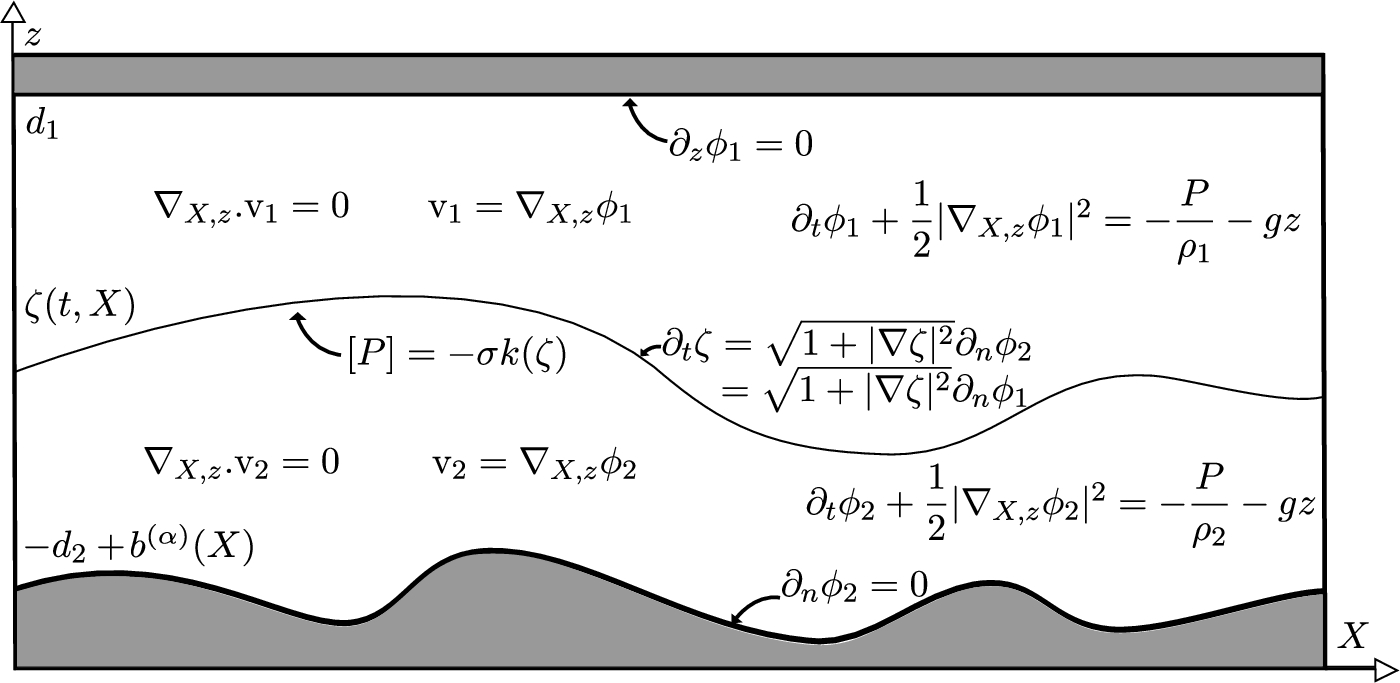
Sketch of the domain and governing equations.

2.1. Full Euler system

We review that the framework comprises two layers of immiscible, homogeneous, perfect, incompressible liquids just affected by gravity (see Fig. 1). We confine ourselves to the bi-dimensional case, i.e. the horizontal dimension $d = 1$ . $ζ (t, x)$ represents the deformation of the interface between the two layers and $b^{(α)} (x) = b (α x)$ represents the deformation of the bottom. $α = \frac{λ}{λ_{b}}$ where λ is a characteristic horizontal length (wave-length of the interface); $λ_{b} = \frac{λ}{α}$ is the wave-length of the bottom variations. More precisely, we are interested in specific bottoms wavelength of characteristic order $λ_{b}$ . Then the typical internal wave velocity is given by $\begin{matrix} c_{0} = \sqrt{g \frac{(ρ_{2} - ρ_{1}) d_{1} d_{2}}{ρ_{2} d_{1} + ρ_{1} d_{2}}}, \end{matrix}$ where we denote by $d_{1}$ (resp. $d_{2}$ ) the depth of the upper (resp. lower) layer; and $ρ_{1}$ (resp. $ρ_{2}$ ) the density of the upper (resp. lower) layer, g is the gravitational acceleration.

The study of the asymptotic dynamics is made accessible by the nondimensionalization of the equations.1

¹
The adapted re-scaling is motivated by the study of the linearized system (2.2) around the rest state $(ζ, ψ) = (0, 0)$ and over a flat topography done in [26].

To this end we introduce dimensionless variables and unknowns that reduce the setting to the physical regime under consideration:

\begin{matrix} \tilde{z} : = \frac{z}{d_{1}}, \tilde{X} : = \frac{X}{λ}, \tilde{t} : = \frac{c_{0}}{λ} t, \end{matrix}

and

\begin{array}{l} \tilde{ζ} (\tilde{t}, \tilde{X}) : = \frac{ζ (t, X)}{a}, \tilde{b} (α \tilde{X}) : = \frac{b (X)}{a_{b}}, \\ \tilde{ϕ_{i}} (\tilde{t}, \tilde{X}, \tilde{z}) : = \frac{d_{1}}{a λ c_{0}} ϕ_{i} (t, X, z) (i = 1, 2) . \end{array}

Now we introduce the following dimensionless parameters

\begin{matrix} (2.1) & \begin{matrix} μ : = \frac{d_{1}^{2}}{λ^{2}}, ϵ : = \frac{a}{d_{1}}, β : = \frac{a_{b}}{d_{1}}, δ : = \frac{d_{1}}{d_{2}}, \\ γ = \frac{ρ_{1}}{ρ_{2}}, Bo = \frac{g (ρ_{2} - ρ_{1}) λ^{2}}{σ}, \end{matrix} \end{matrix}

where a (resp.

a_{b}

) is the maximal vertical deformation of the interface (resp. bottom) with respect to its rest position; σ the interfacial tension coefficient and

Bo

the classical Bond number, which measures the ratio of gravity forces over capillary forces.

In the following we use $bo = μ Bo = \frac{g (ρ_{2} - ρ_{1}) d_{1}^{2}}{σ}$ instead of the classical Bond number, $Bo$ . The parameter ϵ is often called non linearity parameter while μ is the shallowness parameter.

The equations governing the evolution of the aforedescribed system in the introduction read (using non-dimensionalized variables and the Zakharov/Craig–Sulem formulation) [11,31]: $\begin{matrix} (2.2) & \{\begin{matrix} \partial_{t} ζ - \frac{1}{μ} G^{μ} ψ = 0, \\ \partial_{t} (H^{μ, δ} ψ - γ \partial_{x} ψ) + (γ + δ) \partial_{x} ζ + \frac{ϵ}{2} \partial_{x} (| H^{μ, δ} ψ |^{2} - γ | \partial_{x} ψ |^{2}) \\ = μ ϵ \partial_{x} N^{μ, δ} - μ \frac{γ + δ}{bo} \frac{\partial_{x} (k (ϵ \sqrt{μ} ζ))}{ϵ \sqrt{μ}}, \end{matrix} \end{matrix}$ where we denote $\begin{matrix} N^{μ, δ} : = \frac{{(\frac{1}{μ} G^{μ} ψ + ϵ (\partial_{x} ζ) H^{μ, δ} ψ)}^{2} - γ {(\frac{1}{μ} G^{μ} ψ + ϵ (\partial_{x} ζ) (\partial_{x} ψ))}^{2}}{2 (1 + μ | ϵ \partial_{x} ζ |^{2})} . \end{matrix}$ ψ represents the trace of the velocity potential of the upper-fluid at the interface.

The function $k (ζ) = - \partial_{x} (\frac{1}{\sqrt{1 + | \partial_{x} ζ |^{2}}} \partial_{x} ζ)$ denotes the mean curvature of the interface.

We will refer to (2.2) as the full Euler system, and solutions of this system will be exact solutions of the problem. We let the reader check [16, Section 2] for more details on the construction of the system.

Finally, we define the so-called Dirichlet–Neumann operators $G^{μ}$ and $H^{μ, δ}$ as follows:

Definition 2.1 (Dirichlet–Neumann operators).

Let $ζ, b \in H^{t_{0} + 1} (R)$ , $t_{0} > 1 / 2$ , such that there exists $h_{0} > 0$ with $1 - ϵ ζ ⩾ h_{0} > 0$ and $\frac{1}{δ} + ϵ ζ - β b^{(α)} ⩾ h_{0} > 0$ , and let $ψ \in L_{loc}^{2} (R), \partial_{x} ψ \in H^{1 / 2} (R)$ . Then we define $\begin{array}{l} G^{μ} ψ : = G^{μ} [ϵ ζ] ψ : = \sqrt{1 + μ | ϵ \partial_{x} ζ |^{2}} (\partial_{n} ϕ_{1}) |_{z = ϵ ζ} = - μ ϵ (\partial_{x} ζ) (\partial_{x} ϕ_{1}) |_{z = ϵ ζ} + (\partial_{z} ϕ_{1}) |_{z = ϵ ζ}, \\ H^{μ, δ} ψ : = H^{μ, δ} [ϵ ζ, β b^{(α)}] ψ : = \partial_{x} (ϕ_{2} |_{z = ϵ ζ}) = (\partial_{x} ϕ_{2}) |_{z = ϵ ζ} + ϵ (\partial_{x} ζ) (\partial_{z} ϕ_{2}) |_{z = ϵ ζ}, \end{array}$ where $ϕ_{1}$ and $ϕ_{2}$ are uniquely defined (up to a constant for $ϕ_{2}$ ) as the solutions in $H^{2} (R)$ of the Laplace’s problems: $\begin{matrix} (2.3) & \{\begin{matrix} (μ \partial_{x}^{2} + \partial_{z}^{2}) ϕ_{1} = 0 & in Ω_{1}, \\ \partial_{z} ϕ_{1} = 0 & on Γ_{t}, \\ ϕ_{1} = ψ & on Γ, \end{matrix} \end{matrix}$ where $Ω_{1} : = {(x, z) \in R^{2}, ϵ ζ (x) < z < 1}$ , $Γ_{t} : = {(x, z) \in R^{2}, z = 1}$ and $Γ : = {(x, z) \in R^{2}, z = ϵ ζ}$ . $\begin{matrix} (2.4) & \{\begin{matrix} (μ \partial_{x}^{2} + \partial_{z}^{2}) ϕ_{2} = 0 & in Ω_{2}, \\ \partial_{n} ϕ_{2} = \partial_{n} ϕ_{1} & on Γ, \\ \partial_{n} ϕ_{2} = 0 & on Γ_{b}, \end{matrix} \end{matrix}$ where $Ω_{2} : = {(x, z) \in R^{2}, - \frac{1}{δ} + β b^{(α)} (x) < z < ϵ ζ}$ and $Γ_{b} : = {(x, z) \in R^{2}, z = - \frac{1}{δ} + β b^{(α)} (x)}$ .

The existence and uniqueness of a solution to (2.3)–(2.4), and therefore the well-posedness of the Dirichlet–Neumann operators follow from classical arguments detailed, for example, in [25]. The strategy is to construct a variational solution to the Laplace equation in the fluid domain. Then, show the link between this variational solution and the one of the elliptic boundary value problem obtained by transforming the fluid domain onto a flat strip, using a diffeomorphism. The choice of a regularizing diffeomorphism is used to derive optimal regularity estimates on the solution. These regularity estimates are then used to construct strong solutions to the original Laplace equation in the fluid domain.

2.2. Green–Naghdi model

In this section, we develop the asymptotic Green–Naghdi model with accuracy $O (μ^{2})$ . Our construction is based on replacing the Dirichlet-to-Neumann operators by their asymptotic expansions, with respect to the shallowness parameter, μ, (see [13,16]). Following [8,9], we choose to write the equations using the shear layer-mean velocity as unknown, which is equivalently defined as $\begin{array}{l} (2.5) & v : = \frac{1}{h_{2} (t, x)} \int_{- \frac{1}{δ} + β b^{(α)} (x)}^{ϵ ζ (t, x)} \partial_{x} ϕ_{2} (t, x, z) d z - \frac{γ}{h_{1} (t, x)} \int_{ϵ ζ (t, x)}^{1} \partial_{x} ϕ_{1} (t, x, z) d z . \end{array}$ As discussed in [15], two main advantages follow the use of such a choice. First, the equation describing the evolution of the deformation of the interface is an exact equation, and not a $O (μ^{2})$ approximation. In fact, as shown in [15] one has that $\frac{1}{μ} G^{μ} ψ = - \partial_{x} (\frac{h_{1} h_{2}}{h_{1} + γ h_{2}} v)$ .

This choice gives also a much better behavior concerning the linear well-posedness. For the unidimensional case and over uneven bottoms these equations couple the deformation of the interface ζ to the shear mean velocity v, and can be written as: $\begin{matrix} (2.6) & \{\begin{matrix} \partial_{t} ζ + \partial_{x} (\frac{h_{1} h_{2}}{h_{1} + γ h_{2}} v) = 0, \\ \partial_{t} (v + μ \overline{Q} [h_{1}, h_{2}] v) + (γ + δ) \partial_{x} ζ + \frac{ϵ}{2} \partial_{x} (\frac{h_{1}^{2} - γ h_{2}^{2}}{{(h_{1} + γ h_{2})}^{2}} v^{2}) \\ = μ ϵ \partial_{x} (\overline{R} [h_{1}, h_{2}] v) + μ \frac{γ + δ}{bo} \partial_{x}^{3} ζ, \end{matrix} \end{matrix}$ where we denote $h_{1} = 1 - ϵ ζ$ and $h_{2} = δ^{- 1} + ϵ ζ - β b^{(α)}$ , as well as $\begin{array}{l} \overline{Q} [h_{1}, h_{2}] V & = T [h_{2}, β b^{(α)}] (\frac{h_{1} V}{h_{1} + γ h_{2}}) - γ T [h_{1}, 0] (\frac{- h_{2} V}{h_{1} + γ h_{2}}) \\ = - \frac{1}{3 h_{2}} \partial_{x} (h_{2}^{3} \partial_{x} (\frac{h_{1} V}{h_{1} + γ h_{2}})) \\ + \frac{1}{2 h_{2}} β α [\partial_{x} (h_{2}^{2} {(\partial_{x} b)}^{(α)} \frac{h_{1} V}{h_{1} + γ h_{2}}) - h_{2}^{2} {(\partial_{x} b)}^{(α)} \partial_{x} (\frac{h_{1} V}{h_{1} + γ h_{2}})] \\ + α^{2} β^{2} {({(\partial_{x} b)}^{(α)})}^{2} (\frac{h_{1} V}{h_{1} + γ h_{2}}) \\ (2.7) & - γ [\frac{1}{3 h_{1}} \partial_{x} (h_{1}^{3} \partial_{x} (\frac{h_{2} V}{h_{1} + γ h_{2}}))], \\ \overline{R} [h_{1}, h_{2}] V & = \frac{1}{2} {(- h_{2} \partial_{x} (\frac{h_{1} V}{h_{1} + γ h_{2}}) + β α {(\partial_{x} b)}^{(α)} (\frac{h_{1} V}{h_{1} + γ h_{2}}))}^{2} \\ - \frac{γ}{2} {(h_{1} \partial_{x} (\frac{- h_{2} V}{h_{1} + γ h_{2}}))}^{2} - (\frac{h_{1} V}{h_{1} + γ h_{2}}) T [h_{2}, β b^{(α)}] (\frac{h_{1} V}{h_{1} + γ h_{2}}) \\ (2.8) & + γ (\frac{- h_{2} V}{h_{1} + γ h_{2}}) T [h_{1}, 0] (\frac{- h_{2} V}{h_{1} + γ h_{2}}), \end{array}$ with $T [h, b^{(α)}] V : = \frac{- 1}{3 h} \partial_{x} (h^{3} \partial_{x} V) + α \frac{1}{2 h} [\partial_{x} (h^{2} {(\partial_{x} b)}^{(α)} V) - h^{2} {(\partial_{x} b)}^{(α)} (\partial_{x} V)] + α^{2} {({(\partial_{x} b)}^{(α)})}^{2} V$ .

Remark 2.2.
We would like to mention that the well posedness result for the original Green–Naghdi model (2.6), has been proved in [18, Section 5] in the flat bottom case with an adaptive change of variable. Their strategy is similar to the one used for the full Euler system with surface tension by Lannes [26]. The main tool of the analysis is the control of a space–time energy.

In what follows, we restrict our study to the following set of dimensionless parameters: $\begin{array}{l} P & : = {p = (μ, ϵ, δ, γ, β, α, bo) : 0 < μ ⩽ μ_{max}, 0 ⩽ ϵ ⩽ 1, \\ δ \in (δ_{min}, δ_{max}), 0 ⩽ γ < 1, 0 ⩽ β ⩽ β_{max}, 0 ⩽ α ⩽ α_{max}, {bo}_{min} ⩽ bo ⩽ \infty}, \end{array}$ with given $\begin{matrix} 0 ⩽ μ_{max}, δ_{min}^{- 1}, δ_{max}, {bo}_{min}^{- 1}, β_{max}, α_{max} < \infty and {bo}_{min} ≫ 6 . \end{matrix}$

We close this section by stating the first rigorous justification of the two-layers Green–Naghdi model, in the sense of consistency. Let us define exactly what we assign by consistency throughout this paper. Definition 2.3.
We say that ${(ζ^{p}, v^{p})}_{p \in P}$ is $L^{\infty}$ -consistent (resp. $H^{s}$ -consistent of order $s ⩾ 0$ ) on $[0, T]$ with an asymptotic model (Σ) at precision $O (μ^{2})$ , if for all $p \in P$ , $(ζ^{p}, v^{p})$ satisfies (Σ), up to a right hand side $μ^{2} R$ with R bounded in $L^{\infty} ([0, T] \times R)$ (resp. in $L^{\infty} ([0, T], H^{s} (R))$ ), uniformly with respect to $t \in [0, T]$ and $p \in P$ .
Remark 2.4.
Since $H^{s} (R)$ is continuously embedded in $L^{\infty} (R)$ when $s > 1 / 2$ , the $H^{s}$ -consistency implies the $L^{\infty}$ -consistency. The notion of $H^{s}$ -consistency is stronger than the notion of $L^{\infty}$ -consistency and allows a full justification of the asymptotic models.
Proposition 2.5 (Consistency).

For $p \in P$ , let $U^{p} = {(ζ^{p}, ψ^{p})}^{⊤}$ be a family of solutions of the full Euler system ( 2.2 ) such that there exists $T > 0$ , $s ⩾ s_{0} + 1$ , $s_{0} > 1 / 2$ for which ${(ζ^{p}, \partial_{x} ψ^{p})}^{⊤}$ is bounded in $L^{\infty} {([0, T); H^{s + N})}^{2}$ with sufficiently large N, and uniformly with respect to $p \in P$ . Moreover assume that $b \in H^{s + N}$ and there exists $h_{01} > 0$ such that $\begin{array}{l} (H1) & h_{1} = 1 - ϵ ζ^{p} ⩾ h_{01} > 0, h_{2} = 1 / δ + ϵ ζ^{p} - β b^{(α)} ⩾ h_{01} > 0 . \end{array}$ Define $v^{p}$ as in ( 2.5 ). Then $(ζ^{p}, v^{p})$ is $H^{s}$ -consistent with ( 2.6 ), on $[0, T]$ with precision $O (μ^{2})$ .

Proof.
The proof of this proposition is obtained as in the proof of [16, Proposition 3.14]. We omit it here. □

3. Construction of the new coupled model

In the following section, we construct a new asymptotic model that shares the same order of precision as the standard one under some restrictions on the set of parameters $p \in P$ , but have a mathematical structure more suitable for the study of its well-posedness. To this end, we use additional assumptions on the deformation of the interface and the deformation of the bottom. The assumptions are as follows: $\begin{matrix} (3.1) & ϵ = O (\sqrt{μ}) and β α = O (\sqrt{μ}) . \end{matrix}$ The following expansions formally hold: $\begin{array}{l} \frac{h_{1}}{h_{1} + γ h_{2}} = \frac{δ}{γ + δ - γ δ β b^{(α)}} (1 - ϵ ζ + \frac{ϵ ζ δ (1 - γ)}{γ + δ - γ δ β b^{(α)}} + O (ϵ^{2})), \\ \frac{h_{2}}{h_{1} + γ h_{2}} = \frac{δ}{γ + δ - γ δ β b^{(α)}} (δ^{- 1} + ϵ ζ - β b^{(α)} + \frac{(1 - δ β b^{(α)}) ϵ ζ (1 - γ)}{γ + δ - γ δ β b^{(α)}} + O (ϵ^{2})) . \end{array}$ Plugging these expansions into $\overline{Q} [h_{1}, h_{2}] v$ and $\overline{R} [h_{1}, h_{2}] v$ , one can check that the following approximations formally hold: $\begin{array}{l} \overline{Q} [h_{1}, h_{2}] v & = - d \partial_{x}^{2} v + ϵ (η v \partial_{x}^{2} ζ + (2 η + (γ - 1) g) \partial_{x} ζ \partial_{x} v + (η + \frac{2}{3} (γ - 1) g) ζ \partial_{x}^{2} v) \\ + β (η_{1} α^{2} {(\partial_{x}^{2} b)}^{(α)} v + 2 η_{1} α {(\partial_{x} b)}^{(α)} \partial_{x} v + (\frac{γ}{3} f + \frac{2}{3} δ^{- 1} f) b^{(α)} \partial_{x}^{2} v) \\ + β^{2} (\frac{2 γ}{3} f^{'} b^{(α)} α {(\partial_{x} b)}^{(α)} \partial_{x} v - \frac{1}{3} f {b^{(α)}}^{2} \partial_{x}^{2} v) + O (ϵ^{2}, ϵ β α, β^{2} α^{2}), \\ \overline{R} [h_{1}, h_{2}] v & = (1 - γ) g^{2} (\frac{1}{2} {(\partial_{x} v)}^{2} + \frac{1}{3} v \partial_{x}^{2} v) + O (ϵ, β α), \end{array}$ with $\begin{array}{l} (3.2) & d = d (β b^{(α)}) = \frac{1 + γ δ}{3 δ (γ + δ - γ δ β b^{(α)})}, \\ (3.3) & f = f (β b^{(α)}) = \frac{δ}{(γ + δ - γ δ β b^{(α)})}, \\ (3.4) & f^{'} = f^{'} (β b^{(α)}) = \frac{γ δ^{2}}{{(γ + δ - γ δ β b^{(α)})}^{2}}, \\ (3.5) & g = g (β b^{(α)}) = \frac{1 - δ β b^{(α)}}{(γ + δ - γ δ β b^{(α)})} \\ (3.6) & η = η (β b^{(α)}) = \frac{1}{3} {(δ^{- 1} - β b^{(α)})}^{2} f - \frac{1}{3} {(δ^{- 1} - β b^{(α)})}^{2} (1 - γ) f^{2} - \frac{γ}{3} f - \frac{γ}{3} f g (1 - γ), \\ (3.7) & η_{1} = η_{1} (β b^{(α)}) = - \frac{1}{3} {(δ^{- 1} - β b^{(α)})}^{2} f^{'} + \frac{(δ^{- 1} - β b^{(α)})}{2} f - \frac{γ}{3} δ^{- 1} f^{'} + \frac{γ}{3} f . \end{array}$ Actually, thanks to the non-zero depth condition (H1) that we assume, one has $h_{1} + h_{2} > 0$ , which is equivalent to say that $β b^{(α)} < 1 + 1 / δ$ . Since $γ < 1$ , one has $β b^{(α)} < \frac{γ + δ}{γ δ}$ , so one can deduce that the above functions are well defined under the non-zero depth condition.

Plugging the expansions of $\overline{Q} [h_{1}, h_{2}] v$ and $\overline{R} [h_{1}, h_{2}] v$ into system (2.6) yields a streamlined model, with the same order of accuracy as the original model (that is $O (μ^{2})$ ). We will use yet a few extra changes, keeping in mind that the end goal is to create an equivalent model (again, in the sense of consistency), which has a structure like symmetrizable quasilinear systems.

The first step is to introduce the following symmetric operator, $\begin{matrix} (3.8) & T [ϵ ζ, β b^{(α)}] V = q_{1} V - μ \partial_{x} (ν q_{2} \partial_{x} V), \end{matrix}$ where $q_{1} : = 1 + ϵ κ_{1} (β b^{(α)}) ζ + ω_{1} (β b^{(α)})$ and $q_{2} : = 1 + ϵ κ_{2} (β b^{(α)}) ζ + ω_{2} (β b^{(α)})$ .

We denote by $ν, κ_{1}, κ_{2}, ω_{1}, ω_{2}$ functions depending on $β b^{(α)}$ to be precisely determined in order to cancel the high order derivatives on ζ which cannot be controlled by the considered energy space. In order to deal with these terms, we introduce $T [ϵ ζ, β b] \partial_{t} v$ . Here and in the following, we omit the dependence on $β b^{(α)}$ for the sake of readability so as to write, $\begin{array}{l} T [ϵ ζ, β b] \partial_{t} v - q_{1} \partial_{t} (v + μ \overline{Q} [h_{1}, h_{2}] v) + q_{1} μ \frac{γ + δ}{bo} \partial_{x}^{3} ζ \\ = - μ \partial_{x} ν \partial_{x} \partial_{t} v - μ ν \partial_{x}^{2} \partial_{t} v - μ \partial_{x} (ν ϵ κ_{2} ζ \partial_{x} \partial_{t} v) - μ \partial_{x} (ν ω_{2} \partial_{x} \partial_{t} v) \\ - μ \partial_{t} \overline{Q} [h_{1}, h_{2}] v - μ ϵ κ_{1} ζ \partial_{t} \overline{Q} [h_{1}, h_{2}] v \\ - μ ω_{1} \partial_{t} \overline{Q} [h_{1}, h_{2}] v + μ \frac{γ + δ}{bo} \partial_{x}^{3} ζ + μ ϵ κ_{1} ζ \frac{γ + δ}{bo} \partial_{x}^{3} ζ \\ (3.9) & + μ ω_{1} \frac{γ + δ}{bo} \partial_{x}^{3} ζ + O (μ^{2}, μ ϵ^{2}, μ ϵ β α, μ β^{2} α^{2}) . \end{array}$ The first order ( $μ \partial_{x}^{2} \partial_{t} v$ ) term may be canceled with a proper choice of ν, making use of the fact that the second equation of system (2.6) yields $\begin{matrix} \partial_{t} v = - (γ + δ) \partial_{x} ζ - \frac{ϵ}{2} (f^{2} - γ g^{2}) \partial_{x} (| v |^{2}) + O (ϵ^{2}, ϵ β α, μ) . \end{matrix}$ Indeed, it follows that $\begin{matrix} μ \frac{γ + δ}{bo} \partial_{x}^{3} ζ = \frac{- μ}{bo} \partial_{x}^{2} \partial_{t} v - \frac{μ ϵ}{2 bo} (f^{2} - γ g^{2}) \partial_{x}^{3} (| v |^{2}) + O (μ ϵ^{2}, μ ϵ β α, μ^{2}) . \end{matrix}$ After replacing the term $μ \frac{γ + δ}{bo} \partial_{x}^{3} ζ$ of the equation (3.9) by its expression given above and taking the identification of $\partial_{t} \overline{Q} [h_{1}, h_{2}] v$ using (2.7), thus one defines $\begin{matrix} (3.10) & ν = ν (β b^{(α)}) = d - \frac{1}{bo} . \end{matrix}$ Using again that (2.6) yields: $\begin{matrix} \partial_{t} v = - (γ + δ) \partial_{x} ζ + O (ϵ, μ) \end{matrix}$ and $\begin{matrix} \partial_{t} ζ = - g \partial_{x} v + O (ϵ, β α, μ), \end{matrix}$ it becomes clear now, that one can adjust $κ_{1}, κ_{2}, ω_{1}, ω_{2}$ so that all terms involving ζ and its derivatives are canceled. More specifically we set, $\begin{array}{l} κ_{2} & = κ_{2} (β b^{(α)}) \\ (3.11) & = \frac{- (3 η + (γ - 1) g) (1 + ω_{1})}{ν}, \end{array}$ so that $\partial_{x} ζ \partial_{x}^{2} ζ$ terms are canceled.

In order to deal with the $ζ \partial_{x}^{3} ζ$ terms we set $κ_{1}$ so that, $\begin{matrix} ν κ_{2} + (1 + ω_{1}) (η + \frac{2}{3} (γ - 1) g) - ν κ_{1} + β b^{(α)} κ_{1} (\frac{γ}{3} f + \frac{2}{3} δ^{- 1} f) - β^{2} {b^{(α)}}^{2} κ_{1} \frac{f}{3} = 0 . \end{matrix}$ Using (3.11), one defines $\begin{array}{rcl} κ_{1} & = & κ_{1} (β b^{(α)}) \\ (3.12) & = & \frac{(- 2 η - \frac{(γ - 1)}{3} g) (1 + ω_{1})}{ν - β b^{(α)} (\frac{γ}{3} f + \frac{2}{3} δ^{- 1} f) + \frac{β^{2} {b^{(α)}}^{2}}{3} f} . \end{array}$ In order to deal with the $\partial_{x}^{3} ζ$ terms, $ω_{1}$ is determined as follows, $\begin{array}{l} (3.13) & ω_{1} & = ω_{1} (β b^{(α)}) = \frac{ν ω_{2} + β b^{(α)} (\frac{γ}{3} f + \frac{2}{3} δ^{- 1} f) - \frac{β^{2} {b^{(α)}}^{2}}{3} f}{ν - β b^{(α)} (\frac{γ}{3} f + \frac{2}{3} δ^{- 1} f) + \frac{β^{2} {b^{(α)}}^{2}}{3} f} . \end{array}$ The ${(\partial_{x} b)}^{(α)} \partial_{x}^{2} ζ$ terms may be canceled with the proper choice of $ω_{2}$ solution of the following first order linear differential equation. $\begin{matrix} (3.14) & ν^{'} ω_{2} + ν ω_{2}^{'} = - ν^{'} - 2 η_{1} (1 + ω_{1}) - \frac{2 γ}{3} f^{'} β b^{(α)} (1 + ω_{1}) . \end{matrix}$ Making use of (3.13), one can easily remark that (3.14) can be written as: $\begin{array}{l} ω_{2}^{'} + \frac{ν^{'}}{ν} ω_{2} + (\frac{(2 η_{1} + β b^{(α)} \frac{2 γ}{3} f^{'})}{ν - β b^{(α)} (\frac{γ}{3} f + \frac{2}{3} δ^{- 1} f) + \frac{β^{2} {b^{(α)}}^{2}}{3} f}) ω_{2} \\ (3.15) & = - \frac{(2 η_{1} + β b^{(α)} \frac{2 γ}{3} f^{'}) β b^{(α)} (\frac{γ}{3} f + \frac{2}{3} δ^{- 1} f - \frac{β b^{(α)}}{3} f)}{ν [ν - β b^{(α)} (\frac{γ}{3} f + \frac{2}{3} δ^{- 1} f) + \frac{β^{2} {b^{(α)}}^{2}}{3} f]} - \frac{ν^{'}}{ν} - \frac{2 η_{1}}{ν} - \frac{2 γ}{3 ν} f^{'} β b^{(α)} . \end{array}$ In order to solve (3.15) and to define $κ_{1}$ , $κ_{2}$ , $ω_{1}$ and $ω_{2}$ we seek for sufficient conditions. Let us shortly detail these conditions namely (H0).

Since $γ ⩾ 0$ , $δ > 0$ and $bo ≫ 6$ then the discriminant of $[ν - β b^{(α)} (\frac{γ}{3} f + \frac{2}{3} δ^{- 1} f) + \frac{β^{2} {b^{(α)}}^{2}}{3} f]$ is $Δ = [γ^{2} δ^{4} bo (bo - 6) + 12 δ^{4} bo + 9 γ^{2} δ^{4}] > 0$ thus one needs: $\begin{array}{l} (H0) & ν (β b^{(α)}) \neq 0, β b^{(α)} \neq \frac{2 δ bo + γ δ^{2} bo - 3 γ δ^{2}}{2 δ^{2} bo} \pm \frac{Δ}{2 δ^{2} bo} . \end{array}$ These conditions simply consist in assuming additional restrictions on the deformation of the bottom. However, one of the remaining terms in (3.9), as well as in $\partial_{x} (\overline{R} [h_{1}, h_{2}] v)$ , involves three derivatives on v. In order to deal with these terms, we introduce $T [ϵ ζ, β b^{(α)}] (ϵ ς v \partial_{x} v)$ where, again, ς is a function of $β b^{(α)}$ to be determined. More precisely, one has $\begin{array}{l} T [ϵ ζ, β b^{(α)}] (ϵ ς v \partial_{x} v) + μ ϵ q_{1} \partial_{x} (\overline{R} [h_{1}, h_{2}] v) \\ (3.16) & = q_{1} (ϵ ς v \partial_{x} v) - μ \partial_{x} (ν q_{2} \partial_{x} (ϵ ς v \partial_{x} v)) + μ ϵ q_{1} \partial_{x} (\overline{R} [h_{1}, h_{2}] v) . \end{array}$ Combining (3.9) with (3.16), one can check that if we set ς such that $\begin{array}{l} ν (1 + ω_{2}) ς & = \frac{(1 - γ) g^{2}}{3} (1 + ω_{1}) - \frac{1}{bo} (f^{2} - γ g^{2}) + η g (1 + ω_{1}) + ν ω_{2} (f^{2} - γ g^{2}) \\ + (1 + ω_{1}) [β b^{(α)} (\frac{γ}{3} f + \frac{2}{3} δ^{- 1} f) (f^{2} - γ g^{2})] \\ (3.17) & - (1 + ω_{1}) [β^{2} {b^{(α)}}^{2} \frac{1}{3} f (f^{2} - γ g^{2})] - ω_{1} d (f^{2} - γ g^{2}), \end{array}$ then the following approximation holds: $\begin{array}{l} T (\partial_{t} v + ϵ ς v \partial_{x} v) - q_{1} \partial_{t} (v + μ (\overline{Q} [h_{1}, h_{2}] v)) + q_{1} μ \frac{γ + δ}{bo} \partial_{x}^{3} ζ + μ ϵ q_{1} \partial_{x} (\overline{R} [h_{1}, h_{2}] v) \\ = q_{1} (ϵ ς v \partial_{x} v) + μ \frac{2 ϵ}{3} (1 + ω_{1}) (γ - 1) g^{2} \partial_{x} ({(\partial_{x} v)}^{2}) \\ (3.18) & + μ β (γ + δ) (1 + ω_{1}) η_{1} α^{2} {(\partial_{x}^{2} b)}^{(α)} \partial_{x} ζ + O (μ^{2}, μ ϵ^{2}, μ ϵ β α, μ β^{2} α^{2}) . \end{array}$

After multiplying the second equation of (2.6) by $q_{1}$ and plugging the expansion (3.18), we obtain the following system of equations: $\begin{matrix} (3.19) & \{\begin{matrix} \partial_{t} ζ + \partial_{x} (\frac{h_{1} h_{2}}{h_{1} + γ h_{2}} v) = 0, \\ T [ϵ ζ, β b] (\partial_{t} v + ϵ ς v \partial_{x} v) + (γ + δ) q_{1} \partial_{x} ζ + \frac{ϵ}{2} q_{1} \partial_{x} (\frac{h_{1}^{2} - γ h_{2}^{2}}{{(h_{1} + γ h_{2})}^{2}} | v |^{2}) - q_{1} (ϵ ς v \partial_{x} v) \\ = μ \frac{2 ϵ}{3} (1 + ω_{1}) (γ - 1) g^{2} \partial_{x} ({(\partial_{x} v)}^{2}) + μ β (γ + δ) (1 + ω_{1}) η_{1} α^{2} {(\partial_{x}^{2} b)}^{(α)} \partial_{x} ζ, \end{matrix} \end{matrix}$ where ς, $ω_{1}$ and $η_{1}$ are defined in (3.17), (3.13) and (3.7). We will refer to (3.19) as the new Green–Naghdi model.

Remark 3.1.
After setting $β = 0$ in (3.19), we recover the model obtained and fully justified by Duchêne, Israwi and Talhouk in [17]. If we take $β = O (\sqrt{μ})$ and $α = 1$ in (3.19), we recover the model obtained and fully justified in [27].

4. Preliminary results

In the following, we seek for sufficient conditions to ensure the strong ellipticity of the operator $T$ which will drive us to the well-posedness and continuity of the inverse $T^{- 1}$ . We recall the operator $T [ϵ ζ, β b]$ , defined in (3.8): $\begin{matrix} (4.1) & T [ϵ ζ, β b^{(α)}] V = q_{1} V - μ \partial_{x} (ν q_{2} \partial_{x} V), \end{matrix}$ with $ν, κ_{1}, κ_{2}, ω_{1}, ω_{2}$ functions depending on $β b^{(α)}$ defined respectively in (3.10), (3.12), (3.11), (3.13), (3.14). In what follows we assume that $ν (β b^{(α)}) > 0$ is bounded from below (by hypothesis): $\begin{matrix} ν (β b^{(α)}) = d (β b^{(α)}) - \frac{1}{bo} ⩾ ν_{0} > 0 . \end{matrix}$ Let us recall the non-zero depth condition $\exists h_{01} > 0$ , such that $\begin{matrix} (H1) & inf_{x \in R} h_{1} ⩾ h_{01} > 0, inf_{x \in R} h_{2} ⩾ h_{01} > 0, \end{matrix}$ where $h_{1} = 1 - ϵ ζ$ and $h_{2} = \frac{1}{δ} + ϵ ζ - β b^{(α)}$ are the depth of respectively the upper and the lower layer of the fluid.

In the same way, we introduce the condition, $\exists h_{02} > 0$ , such that $\begin{array}{l} (H2) & inf_{x \in R} q_{1} ⩾ h_{02} > 0; inf_{x \in R} q_{2} ⩾ h_{02} > 0 . \end{array}$ Actually, this condition, namely (H2) (and similarly the classical non-zero depth condition, (H1)) simply consists in assuming that the deformation of the interface and the one of the bottom are not too large, following the same techniques as in [17] but taking into account the topographic variation.

Before asserting the strong ellipticity of the operator $T$ , let us first introduce $H_{μ}^{s + 1} (R)$ the space $H^{s + 1} (R)$ endowed with the norm $\begin{matrix} | \cdot |_{H_{μ}^{s + 1}}^{2} : = | \cdot |_{H^{s}}^{2} + μ | \cdot |_{H^{s + 1}}^{2} . \end{matrix}$ For $s = 0$ , $| \cdot |_{H_{μ}^{1}}$ is defined as $\begin{matrix} \forall v \in H^{1} (R), | v |_{H_{μ}^{1}}^{2} = | v |_{L^{2}}^{2} + μ | \partial_{x} v |_{L^{2}}^{2}, \end{matrix}$ and is equivalent to the $H^{1} (R)$ -norm but not uniformly with respect to μ. We define by ${(H_{μ}^{1} (R))}^{⋆}$ the space $H^{- 1} (R)$ the dual space of $H_{μ}^{1} (R)$ .

The preliminary results proved in [17, Section 5] remain valid for the operator $T [ϵ ζ, β b^{(α)}]$ . Let us recall the strong ellipticity and invertibility results on $T$ .

Lemma 4.1.
Let $p \in P$ satisfy ( 3.1 ) and $ζ \in L^{\infty} (R)$ , $b^{(α)} \in L^{\infty} (R)$ such that ( H2 ) is satisfied. Then the operator $\begin{matrix} T [ϵ ζ, β b^{(α)}] : H_{μ}^{1} (R) ⟶ {(H_{μ}^{1} (R))}^{⋆} \end{matrix}$ is uniformly continuous and coercive. More precisely, there exists $c_{0} > 0$ such that $\begin{array}{rcl} (4.2) & (T u, v) & ⩽ & c_{0} | u |_{H_{μ}^{1}} | v |_{H_{μ}^{1}}; \\ (4.3) & (T u, u) & ⩾ & \frac{1}{c_{0}} | u |_{H_{μ}^{1}}^{2} \end{array}$ with $c_{0} = C (M, h_{02}^{- 1}, ϵ | ζ |_{L^{\infty}}, β | b^{(α)} |_{L^{\infty}})$ .

We denote for convenience, $M \equiv max {μ_{max}, δ_{min}^{- 1}, δ_{max}, {bo}_{min}^{- 1}, β_{max}, α_{max}, ν_{0}^{- 1}}$ .
Proof.
Let us define the bilinear form $\begin{array}{l} (u, v) = (T u, v) = ((1 + ϵ κ_{1} ζ + ω_{1}) u, v) + μ (ν (1 + ϵ κ_{2} ζ + ω_{2}) \partial_{x} u, \partial_{x} v), \end{array}$ where $(\cdot, \cdot)$ denotes the $L^{2}$ inner product. It is straightforward to check that $\begin{matrix} | a (u, v) | ⩽ sup_{x \in R} | 1 + ϵ κ_{1} ζ + ω_{1} | (u, v) + μ sup_{x \in R} | ν (1 + ϵ κ_{2} ζ + ω_{2}) | (\partial_{x} u, \partial_{x} v), \end{matrix}$ so that (4.2) is now straightforward, by Cauchy–Schwarz inequality.

The $H_{μ}^{1} (R)$ -coercivity of $a (\cdot, \cdot)$ , inequality (4.3), is a consequence of condition (H2): $\begin{array}{l} a (u, u) & = (T u, u) \\ = \int_{R} (1 + ϵ κ_{1} ζ + ω_{1}) | u |^{2} d x + μ \int_{R} ν (1 + ϵ κ_{2} ζ + ω_{2}) | u_{x} |^{2} d x, \\ a (u, u) & ⩾ h_{02} min (1, ν_{0}) | u |_{H_{μ}^{1}}^{2} . \end{array}$ □

The following lemma offers an important invertibility result on $T$ . Lemma 4.2.
Let $p \in P$ satisfy ( 3.1 ) and $ζ \in L^{\infty} (R)$ , $b^{(α)} \in L^{\infty} (R)$ such that ( H2 ) is satisfied. Then the operator $\begin{matrix} T [ϵ ζ, β b^{(α)}] : H^{2} (R) ⟶ L^{2} (R) \end{matrix}$ is bijective.
Proof.
To show the invertibility of $T$ we use the Lax–Milgram theorem. From the previous lemma, we know that the bilinear form: $\begin{array}{l} a (u, v) & = (T u, v) \\ = ((1 + ϵ κ_{1} ζ + ω_{1}) u, v) + μ (ν (1 + ϵ κ_{2} ζ + ω_{2}) \partial_{x} u, \partial_{x} v) \end{array}$ is continuous and uniformly coercive on $H_{μ}^{1} (R)$ . For any $μ > 0$ , the dual of $H_{μ}^{1} (R)$ is $H^{- 1} (R)$ , of whom $L^{2} (R)$ is a subspace, and one has $(f, g) ⩽ | f |_{H_{μ}^{1}} | g |_{L^{2}}$ , independently of $μ > 0$ . Therefore, using Lax–Milgram lemma, for all $f \in L^{2} (R)$ , there exists a unique $u \in H_{μ}^{1} (R)$ such that, for all $v \in H_{μ}^{1} (R)$ $\begin{matrix} a (u, v) = (f, v); \end{matrix}$ equivalently, there is a unique variational solution to the equation $\begin{matrix} (4.4) & T u = f . \end{matrix}$ We then get from the definition of $T$ that $\begin{array}{l} μ ν (1 + ϵ κ_{2} ζ + ω_{2}) \partial_{x}^{2} u \\ = (1 + ϵ κ_{1} ζ + ω_{1}) u - μ \partial_{x} (ν q_{2}) \partial_{x} u - f . \end{array}$ Now, using condition (H2), and since $u \in H^{1} (R)$ , $ζ \in L^{\infty} (R)$ and $f \in L^{2} (R)$ , we deduce that $\partial_{x}^{2} u \in L^{2} (R)$ , and thus $u \in H^{2} (R)$ . We proved that $T [ϵ ζ, β b^{(α)}] : H^{2} (R) ⟶ L^{2} (R)$ is one-to-one and onto. □

5. Linearized system

This section is devoted to the study of the properties of the linearized system associated to our non- linear asymptotic system (3.19), following the classical theory of quasilinear hyperbolic systems. We adapted this study to our new model which takes into account slowly varying topography variations following the same techniques as in [27, Section 5]. We do not state here the energy estimates and refer to [27, Section 5.1] for more details. Let us recall the system (3.19). $\begin{matrix} (5.1) & \{\begin{matrix} \partial_{t} ζ + \partial_{x} (\frac{h_{1} h_{2}}{h_{1} + γ h_{2}} v) = 0, \\ T [ϵ ζ, β b^{(α)}] (\partial_{t} v + ϵ ς v \partial_{x} v) + (γ + δ) q_{1} \partial_{x} ζ \\ + \frac{ϵ}{2} q_{1} \partial_{x} (\frac{h_{1}^{2} - γ h_{2}^{2}}{{(h_{1} + γ h_{2})}^{2}} | v |^{2}) - q_{1} (ϵ ς v \partial_{x} v) \\ = μ \frac{2 ϵ}{3} (1 + ω_{1}) (γ - 1) g^{2} \partial_{x} ({(\partial_{x} v)}^{2}) + μ β (γ + δ) (1 + ω_{1}) η_{1} α^{2} {(\partial_{x}^{2} b)}^{(α)} \partial_{x} ζ, \end{matrix} \end{matrix}$ with $h_{1} = 1 - ϵ ζ$ , $h_{2} = 1 / δ + ϵ ζ - β b^{(α)}$ , $q_{1} : = 1 + ϵ κ_{1} (β b^{(α)}) ζ + ω_{1} (β b^{(α)})$ and $q_{2} : = 1 + ϵ κ_{2} (β b^{(α)}) ζ + ω_{2} (β b^{(α)})$ where $κ_{1}, κ_{2}, ω_{1}, ω_{2}$ and ς are defined in (3.12), (3.11), (3.13), (3.14), (3.17) and $\begin{matrix} T [ϵ ζ, β b] V = q_{1} V - μ \partial_{x} (ν q_{2} \partial_{x} V) . \end{matrix}$ We define the following functions in order to simplify the reading, $\begin{matrix} H : (X, Y) \to \frac{(1 - X) (δ^{- 1} + X - Y)}{1 - X + γ (δ^{- 1} + X - Y)}, \end{matrix}$ and $\begin{matrix} G : (X, Y) \to {(\frac{(1 - X)}{1 - X + γ (δ^{- 1} + X - Y)})}^{2} . \end{matrix}$ One can easily check that $\begin{array}{l} H (ϵ ζ, β b^{(α)}) = \frac{h_{1} h_{2}}{h_{1} + γ h_{2}}, \\ H^{'} (ϵ ζ, β b^{(α)}) = \frac{h_{1}^{2} - γ h_{2}^{2}}{{(h_{1} + γ h_{2})}^{2}}, \\ G (ϵ ζ, β b^{(α)}) = {(\frac{h_{1}}{h_{1} + γ h_{2}})}^{2} . \end{array}$ One can rewrite (5.1), $\begin{matrix} (5.2) & \{\begin{matrix} \partial_{t} ζ + H (ϵ ζ, β b^{(α)}) \partial_{x} v + ϵ \partial_{x} ζ H^{'} (ϵ ζ, β b^{(α)}) v - β α {(\partial_{x} b)}^{(α)} G (ϵ ζ, β b^{(α)}) v = 0, \\ T (\partial_{t} v + \frac{ϵ}{2} ς \partial_{x} (v^{2})) + (γ + δ) q_{1} \partial_{x} ζ \\ + ϵ q_{1} (H^{'} (ϵ ζ, β b^{(α)}) - ς) v \partial_{x} v + ϵ q_{1} \partial_{x} (\frac{H^{'} (ϵ ζ, β b^{(α)})}{2}) v^{2} \\ = μ \frac{2 ϵ}{3} (1 + ω_{1}) (γ - 1) g^{2} \partial_{x} ({(\partial_{x} v)}^{2}) + μ β (γ + δ) (1 + ω_{1}) η_{1} α^{2} {(\partial_{x}^{2} b)}^{(α)} \partial_{x} ζ . \end{matrix} \end{matrix}$ with $\begin{array}{l} \partial_{x} (\frac{H^{'} (ϵ ζ, β b^{(α)})}{2}) = \frac{- γ ϵ \partial_{x} ζ {(h_{1} + h_{2})}^{2}}{{(h_{1} + γ h_{2})}^{3}} + \frac{γ β α {(\partial_{x} b)}^{(α)} h_{1} (h_{1} + h_{2})}{{(h_{1} + γ h_{2})}^{3}} . \end{array}$ The equations can be written after applying $T^{- 1}$ to the second equation in (5.2) as $\begin{matrix} (5.3) & \partial_{t} U + A [U] \partial_{x} U + B [U] = 0, \end{matrix}$ with $\begin{array}{l} (5.4) & A [U] = (\begin{matrix} ϵ H^{'} (ϵ ζ, β b^{(α)}) v & H (ϵ ζ, β b^{(α)}) \\ T^{- 1} (Q \cdot) & T^{- 1} (Q \cdot) + ϵ ς v \cdot \end{matrix}), \\ (5.5) & B [U] = (\begin{matrix} - α β {(\partial_{x} b)}^{(α)} G (ϵ ζ, β b^{(α)}) v \\ T^{- 1} (\frac{γ ϵ β α q_{1} h_{1} (h_{1} + h_{2}) {(\partial_{x} b)}^{(α)}}{{(h_{1} + γ h_{2})}^{3}} v^{2}) \end{matrix}), \end{array}$ where $Q = Q_{0} (ϵ ζ, β b^{(α)}) + Q_{1} (ϵ ζ, β b^{(α)}, v)$ with $Q_{0} (ϵ ζ, β b^{(α)}), Q_{1} (ϵ ζ, β b^{(α)}, v)$ defined as $\begin{array}{l} Q_{0} (ϵ ζ, β b^{(α)}) = (γ + δ) q_{1} - μ β (γ + δ) (1 + ω_{1}) η_{1} α^{2} {(\partial_{x}^{2} b)}^{(α)}, \\ Q_{1} (ϵ ζ, β b^{(α)}, v) = - γ q_{1} (ϵ ζ, β b^{(α)}) \frac{{(h_{1} + h_{2})}^{2}}{{(h_{1} + γ h_{2})}^{3}} v^{2} \end{array}$ and the operator $Q [ϵ ζ, β b^{(α)}, v]$ defined by $\begin{array}{l} Q f & = Q [ϵ ζ, β b^{(α)}, v] f \\ (5.6) & : = ϵ q_{1} (H^{'} (ϵ ζ, β b^{(α)}) - ς) v f - μ \frac{2 ϵ}{3} (1 + ω_{1}) (γ - 1) g^{2} \partial_{x} (\partial_{x} v f) . \end{array}$

Following the traditional theory of quasilinear hyperbolic systems, the existence and uniqueness result of the initial value problem of the above system will depend on a study of energy estimates, for the linearized system around some reference state $\underline{U} = {(\underline{ζ}, \underline{v})}^{⊤}$ : $\begin{matrix} (5.7) & \{\begin{matrix} \partial_{t} U + A [\underline{U}] \partial_{x} U + B [\underline{U}] = 0, \\ U_{|_{t = 0}} = U_{0} . \end{matrix} \end{matrix}$ Let us first remark that by construction, one has a symmetrizer of the system, given by $\begin{matrix} (5.8) & Z [\underline{U}] = (\begin{matrix} \frac{Q_{0} (ϵ \underline{ζ}, β b^{(α)}) + ϵ^{2} Q_{1} (ϵ \underline{ζ}, β b^{(α)}, \underline{v})}{H (ϵ \underline{ζ}, β b^{(α)})} & 0 \\ 0 & T [ϵ \underline{ζ}, β b^{(α)}] \end{matrix}) . \end{matrix}$ One ought to add an extra assumption to guarantee that our symmetrizer is defined and positive which is: $\exists h_{03} > 0$ such that $\begin{matrix} (H3) & Q_{0} (ϵ \underline{ζ}, β b^{(α)}) + ϵ^{2} Q_{1} (ϵ \underline{ζ}, β b^{(α)}, \underline{v}) ⩾ h_{03} > 0 . \end{matrix}$ After setting $β = 0$ (flat bottom) in H3, one may recover the same assumption as in [17] to ensure that the symmetrizer is defined and positive. Note also that in the flat bottom case this assumption may be seen as the hyperbolicity condition for the first order ( $μ = 0$ ) shallow-water system; see [19].

For given $s ⩾ 0$ and $μ, T > 0$ , we denote by $X^{s}$ the vector space $H^{s} (R) \times H_{μ}^{s + 1} (R)$ endowed with the norm $\forall U = (ζ, v) \in X^{s}$ , $\begin{matrix} | U |_{X^{s}}^{2} : = | ζ |_{H^{s}}^{2} + | v |_{H^{s}}^{2} + μ | \partial_{x} v |_{H^{s}}^{2} . \end{matrix}$ A natural energy for the initial value problem (5.7) is now given by: $\begin{array}{l} E^{s} {(U)}^{2} & = (Λ^{s} U, Z [\underline{U}] Λ^{s} U) \\ = (Λ^{s} ζ, \frac{Q_{0} (ϵ \underline{ζ}, β b^{(α)})}{H (ϵ \underline{ζ}, β b^{(α)})} Λ^{s} ζ) \\ (5.9) & + (Λ^{s} ζ, \frac{ϵ^{2} Q_{1} (ϵ \underline{ζ}, β b^{(α)}, \underline{v})}{H (ϵ \underline{ζ}, β b^{(α)})} Λ^{s} ζ) + (Λ^{s} v, T [ϵ \underline{ζ}, β b^{(α)}] Λ^{s} v) . \end{array}$ In order to ensure the equivalence of $X^{s}$ -norm with the energy of the symmetrizer it requires to add the additional assumption given in (H3). The proof of the equivalence of the $X^{s}$ -norm and the energy of the symmetrizer is a straightforward application of Lemma 4.1 using the additional assumption (H3). We do not detail the proof here and refer to [27, Lemma 5.2].

6. Full justification of the new coupled model

In the words of [25], the full justification of an asymptotic model follows from two requirements. The first one is that the Cauchy problem for both the full Euler system and the asymptotic model should be well-posed for a given class of initial data, and over the relevant time scale; and the second one is that the solutions with corresponding initial data should remain close. In this section we express every one of the elements for the full justification of our model. We do not state the detailed proofs of the following results since they are proved using the same techniques as in [27] adapted to our new model. However we will give the main ideas behind the proofs of these results. Using the consistency result of the Green–Naghdi model stated in Proposition 2.5 and after checking that all terms neglected in the construction of the new coupled model (see Section 3) can be rigorously estimated in the same way, we prove that the full Euler system is consistent with our model (in the sense of Definition 2.3). The obtained model possesses a structure similar to symmetrizable quasilinear systems that allows the study of the properties, and in particular energy estimates, for the linearized system, thus allowing its well-posedness, following the classical theory of hyperbolic systems using an iterative scheme of Picard. Thanks to an energy estimate of the difference of two solutions of the model, we show that our model is stable with respect to the perturbations of the equations. Finally, we prove that the solutions of our system approach the solutions of the full Euler system, with as good a precision as μ is small. This last step is a consequence of the consistency and stability results.

Proposition 6.1 (Consistency).

For all family $P$ of parameters $p$ satisfying ( 3.1 ), let $U^{p} = {(ζ^{p}, ψ^{p})}^{⊤}$ be a family of solutions of the full Euler system ( 2.2 ) such that there exists $T > 0$ , $s ⩾ s_{0} + 1$ , $s_{0} > 1 / 2$ for which ${(ζ^{p}, \partial_{x} ψ^{p})}^{⊤}$ is bounded in $L^{\infty} {([0, T); H^{s + N})}^{2}$ with sufficiently large N, and uniformly with respect to $p$ . Moreover assume that $b \in H^{s + N}$ satisfy ( H0 ) and there exists $h_{01} > 0$ such that $\begin{array}{l} h_{1} = 1 - ϵ ζ^{p} ⩾ h_{01} > 0, h_{2} = \frac{1}{δ} + ϵ ζ^{p} - β b^{(α)} ⩾ h_{01} > 0 . \end{array}$ Define $v^{p}$ as in ( 2.5 ). Then $(ζ^{p}, v^{p})$ is $H^{s}$ -consistent with ( 3.19 ), on $[0, T]$ with precision $O (μ^{2})$ .

Before stating the existence and uniqueness result we would like to mention that the assumptions (H1), (H2) and (H3) are imposed only on the initial data. It is a consequence of the work [27, Theorem 6.1] that these assumptions will remain true over the relevant time scale.

Theorem 6.2 (Existence and uniqueness).

Let $p \in P$ satisfy ( 3.1 ) and $s ⩾ s_{0} + 1$ , $s_{0} > 1 / 2$ , and assume $U_{0} = {(ζ_{0}, v_{0})}^{⊤} \in X^{s}$ , $b \in H^{s + 1}$ satisfies ( H0 ), ( H1 ), ( H2 ), and ( H3 ). Then there exists a maximal time $T_{max} > 0$ , uniformly bounded from below with respect to $p \in P$ , such that the system of equations ( 3.19 ) admits a unique strong solution $U = {(ζ, v)}^{⊤} \in C^{0} ([0, T_{max}); X^{s}) \cap C^{1} ([0, T_{max}); X^{s - 1})$ with the initial value $(ζ, v) |_{t = 0} = (ζ_{0}, v_{0})$ , and preserving the conditions ( H1 ), ( H2 ) and ( H3 ) (with different lower bounds) for any $t \in [0, T_{max})$ .

Moreover, there exists T, λ and $C_{0} = C (h_{01}^{- 1}, h_{02}^{- 1}, h_{03}^{- 1}, M, T, | U_{0} |_{X^{s}}, | b |_{H^{s + 1}})$ , such that $T_{max} ⩾ \frac{T}{max (ϵ, β α)}$ , and one has the energy estimates $\forall 0 ⩽ t ⩽ \frac{T}{max (ϵ, β α)}$ , $\begin{array}{l} {| U (t, \cdot) |}_{X^{s}} + {| \partial_{t} U (t, \cdot) |}_{X^{s - 1}} \\ ⩽ C_{0} e^{max (ϵ, β α) λ t} + max (ϵ, β α) C_{0}^{2} \int_{0}^{t} e^{max (ϵ, β α) λ (t - t^{'})} d t^{'} + max (ϵ, β α) C_{0} . \end{array}$ If $T_{max} < \infty$ , one has either $\begin{matrix} {| U (t, \cdot) |}_{X^{s}} ⟶ \infty as t ⟶ T_{max}, \end{matrix}$ or one of the conditions ( H1 ), ( H2 ), ( H3 ) ceases to be true as $t ⟶ T_{max}$ .

Theorem 6.3 (Stability).

Let $p \in P$ satisfy ( 3.1 ) and $s ⩾ s_{0} + 1$ with $s_{0} > 1 / 2$ , and assume $U_{1, 0} = {(ζ_{1, 0}, v_{1, 0})}^{⊤} \in X^{s}$ , $U_{2, 0} = {(ζ_{2, 0}, v_{2, 0})}^{⊤} \in X^{s + 1}$ , and $b \in H^{s + 1}$ satisfies ( H0 ), ( H1 ), ( H2 ), and ( H3 ). Denote $U_{j}$ the solution to ( 3.19 ) with $U_{j} |_{t = 0} = U_{j, 0}$ .

Then there exists $T, λ$ , $C_{0} = C (M, h_{01}^{- 1}, h_{02}^{- 1}, h_{03}^{- 1}, | U_{1, 0} |_{X^{s}}, | U_{2, 0} |_{X^{s + 1}}, | b |_{H^{s + 1}})$ such that $\forall t \in [0, \frac{T}{max (ϵ, β α)}]$ , $\begin{matrix} {| (U_{1} - U_{2}) (t, \cdot) |}_{X^{s}} ⩽ C_{0} e^{max (ϵ, β α) λ t} | U_{1, 0} - U_{2, 0} |_{X^{s}} . \end{matrix}$

Theorem 6.4 (Convergence).

Let $p \in P$ satisfy ( 3.1 ) and $s ⩾ s_{0} + 1$ with $s_{0} > 1 / 2$ , and let $U^{0} : = {(ζ^{0}, ψ^{0})}^{⊤} \in H^{s + N} {(R)}^{2}$ , $b \in H^{s + N}$ satisfy the hypotheses ( H0 ), ( H1 ), ( H2 ), and ( H3 ), with N sufficiently large. We suppose $U : = {(ζ, ψ)}^{⊤}$ a unique solution to the full Euler system ( 2.2 ) with initial data ${(ζ^{0}, ψ^{0})}^{⊤}$ , defined on $[0, T_{1}]$ for $T_{1} > 0$ 1

¹
To our knowledge, the local well-posedness of the full Euler system in the two-fluid configuration over a variable topography seems to be an open problem.

, and we suppose that

U : = {(ζ, ψ)}^{⊤}

satisfies the assumptions of our consistency result, Proposition ( 6.1 ). Then there exists

C, T > 0

, independent of

p

, such that

There exists a unique solution $\underline{U} : = {(\underline{ζ}, \underline{v})}^{⊤}$ to our new model ( 3.19 ), defined on $[0, \frac{T}{max (ϵ, β α)}]$ and with initial data ${(ζ^{0}, v^{0})}^{⊤}$ (provided by Theorem 6.2 );

With v, defined as in ( 2.5 ), one has for any $t ⩽ min (T_{1}, \frac{T}{max (ϵ, β α)})$ , $\begin{matrix} {| (ζ, v) - (\underline{ζ}, \underline{v}) |}_{L^{\infty} ([0, t]; X^{s})} ⩽ C μ^{2} t . \end{matrix}$

7. Derivation of the unidirectional approximation

In what follows, we are interested in scalar asymptotic models for the propagation of internal waves instead of coupled models which consist in a system of evolution equations. Thus, we derive an approximate solution to the Green–Naghdi system (2.6) over variable topography, taking after the same strategy created for the water-wave problem in [10], and for the internal wave problem over flat topography in [15]. In fact, at the lowest order of approximation (that is dropping the first order terms in μ, ϵ and β), the Green–Naghdi system (2.6) becomes a linear wave equation of speed $\pm 1$ and any initial disturbance of the interface splits up into two waves moving in opposite direction. In what follows we will focus on a given direction of the two counter-propagating waves.

More precisely, we prove that if one picks carefully the initial data (deformation of the interface as well as shear layer-mean velocity) so that only one wave is present in the dynamics of the system, then the flow is unidirectional, in the sense that the flow can be approximated as a solution of a scalar evolution equation for the deformation at the interface (see (7.8)), followed by a reconstruction of the shear layer-mean velocity from the deformation (in particular, the initial shear velocity is determined by the initial deformation).

Let us now state the steps for the derivation of the unidirectional approximation. In the interest of simplifying the calculations, we use the Green–Naghdi system (2.6) expressed using the variables $(ζ, \underline{v})$ , where we define $\underline{v} = \frac{h_{1} h_{2}}{h_{1} + γ h_{2}} v$ . The system reads $\begin{matrix} (7.1) & \{\begin{matrix} \partial_{t} ζ + \partial_{x} \underline{v} = 0, \\ \partial_{t} (\frac{h_{1} + γ h_{2}}{h_{1} h_{2}} \underline{v} + μ \underline{Q} [h_{1}, h_{2}] \underline{v}) + (γ + δ) \partial_{x} ζ + \frac{ϵ}{2} \partial_{x} (\frac{h_{1}^{2} - γ h_{2}^{2}}{{(h_{1} h_{2})}^{2}} {\underline{v}}^{2}) \\ = μ ϵ \partial_{x} (\underline{R} [h_{1}, h_{2}] \underline{v}) + μ \frac{γ + δ}{bo} \partial_{x}^{3} ζ, \end{matrix} \end{matrix}$ where we denote $\begin{array}{l} \underline{Q} [h_{1}, h_{2}] V & = T [h_{2}, β b^{(α)}] (\frac{1}{h_{2}} V) - γ T [h_{1}, 0] (\frac{- V}{h_{1}}) \\ = - \frac{1}{3 h_{2}} \partial_{x} (h_{2}^{3} \partial_{x} (\frac{V}{h_{2}})) \\ + \frac{1}{2 h_{2}} β α [\partial_{x} (h_{2}^{2} {(\partial_{x} b)}^{(α)} \frac{V}{h_{2}}) - h_{2}^{2} {(\partial_{x} b)}^{(α)} \partial_{x} (\frac{V}{h_{2}})] \\ (7.2) & + α^{2} β^{2} {({(\partial_{x} b)}^{(α)})}^{2} (\frac{V}{h_{2}}) - γ [\frac{1}{3 h_{1}} \partial_{x} (h_{1}^{3} \partial_{x} (\frac{V}{h_{1}}))], \\ \underline{R} [h_{1}, h_{2}] V & = \frac{1}{2} {(- h_{2} \partial_{x} (\frac{V}{h_{2}}) + β α {(\partial_{x} b)}^{(α)} (\frac{V}{h_{2}}))}^{2} - \frac{γ}{2} {(h_{1} \partial_{x} (\frac{- V}{h_{1}}))}^{2} \\ (7.3) & - (\frac{V}{h_{2}}) T [h_{2}, β b^{(α)}] (\frac{V}{h_{2}}) + γ (\frac{- V}{h_{1}}) T [h_{1}, 0] (\frac{- V}{h_{1}}) . \end{array}$ We proceed by giving the following asymptotic expansions: $\begin{array}{l} (7.4) & \frac{h_{1} + γ h_{2}}{h_{1} h_{2}} = γ + c + ϵ ζ (γ - c^{2}) + ϵ^{2} ζ^{2} (γ + c^{3}) + ϵ^{3} ζ^{3} (γ - c^{4}) + O (ϵ^{4}), \\ (7.5) & \frac{h_{1}^{2} - γ h_{2}^{2}}{{(h_{1} h_{2})}^{2}} = c^{2} - γ - 2 ϵ ζ (c^{3} + γ) + 3 ϵ^{2} ζ^{2} (c^{4} - γ) + O (ϵ^{3}), \\ \underline{Q} [h_{1}, h_{2}] \underline{v} = - d (γ + c) \partial_{x}^{2} \underline{v} - ϵ d (γ - c^{2}) \partial_{x}^{2} (ζ \underline{v}) \\ + ϵ (γ + c) [η \underline{v} \partial_{x}^{2} ζ + (2 η + (γ - 1) g) \partial_{x} ζ \partial_{x} \underline{v} + (η + \frac{2}{3} (γ - 1) g) ζ \partial_{x}^{2} \underline{v}] \\ + β (\frac{γ}{3} f + \frac{2}{3} δ^{- 1} f) b^{(α)} [(γ + c) \partial_{x}^{2} \underline{v} + ϵ (γ - c^{2}) \partial_{x}^{2} (ζ \underline{v})] \\ + β α (γ + c) (2 η_{1} {(\partial_{x} b)}^{(α)} \partial_{x} \underline{v}) - β^{2} \frac{1}{3} f {b^{(α)}}^{2} [(γ + c) \partial_{x}^{2} \underline{v} + ϵ (γ - c^{2}) \partial_{x}^{2} (ζ \underline{v})] \\ (7.6) & + β^{2} α (γ + c) (\frac{2 γ}{3} f^{'} b^{(α)} {(\partial_{x} b)}^{(α)} \partial_{x} \underline{v}) + O (ϵ^{2}, β α ϵ, β α^{3 / 2}), \\ (7.7) & \underline{R} [h_{1}, h_{2}] \underline{v} = (1 - γ) g^{2} {(γ + c)}^{2} [\frac{1}{2} {(\partial_{x} \underline{v})}^{2} + \frac{1}{3} \underline{v} \partial_{x}^{2} \underline{v}] + O (ϵ, β α), \end{array}$ with $c = c (β b^{(α)}) = \frac{δ}{1 - δ β b^{(α)}}$ and $d, f, f^{'}, g, η$ and $η_{1}$ functions depending on $β b^{(α)}$ , defined in (3.2), (3.3), (3.4), (3.5), (3.6) and (3.7). We would like to mention that definition of the function $c (β b^{(α)})$ forbids the value $β b^{(α)} = δ^{- 1}$ . That is to say the bottom should be restricted in a small neighborhood around this value.

Let ζ satisfy the following scalar evolution equation, $\begin{array}{l} \partial_{t} ζ + α_{0} \partial_{x} ζ + \frac{1}{2} \partial_{x} (α_{0}) ζ + ϵ α_{1} ζ \partial_{x} ζ + ϵ^{2} α_{2} ζ^{2} \partial_{x} ζ \\ (7.8) & + ϵ^{3} α_{3} ζ^{3} \partial_{x} ζ + μ ϱ \partial_{x}^{3} ζ + μ β α (ω + ϱ^{'}) {(\partial_{x} b)}^{(α)} \partial_{x}^{2} ζ + μ ϵ \partial_{x} (ϰ_{1} ζ \partial_{x}^{2} ζ + ϰ_{2} {(\partial_{x} ζ)}^{2}) = 0, \end{array}$ where $α_{i}$ ( $i = 0, 1, 2, 3$ ), ϱ, ω, $ϰ_{1}$ and $ϰ_{2}$ are functions depending on $β b^{(α)}$ to be determined later.

In order to satisfy the first equation of (7.1), $\underline{v}$ shall satisfy the following $\begin{array}{l} \underline{v} & = α_{0} ζ - \frac{1}{2} \int_{- \infty}^{x} \partial_{x} (α_{0}) ζ d x + ϵ \frac{α_{1}}{2} ζ^{2} + ϵ^{2} \frac{α_{2}}{3} ζ^{3} + ϵ^{3} \frac{α_{3}}{4} ζ^{4} \\ (7.9) & + μ ϱ \partial_{x}^{2} ζ + μ β α ω {(\partial_{x} b)}^{(α)} \partial_{x} ζ + μ ϵ (ϰ_{1} ζ \partial_{x}^{2} ζ + ϰ_{2} {(\partial_{x} ζ)}^{2}) . \end{array}$ In fact, applying the first order space derivative to $\underline{v}$ and adding it to $\partial_{t} ζ$ term, one recover (7.8), after neglecting the $O (β α ϵ, β α^{3 / 2})$ terms and using the fact that the system is at rest at infinity: $(ζ, \underline{v} \to 0 when x \to \pm \infty)$ .

We will proceed now by showing that the coefficients $α_{i}$ ( $i = 0, 1, 2, 3$ ), ϱ, ω, $ϰ_{1}$ and $ϰ_{2}$ are precisely chosen so that the second equation of (7.1) is satisfied up to a remainder term $R$ of size $O (μ^{2}, μ ϵ^{2}, β α^{3 / 2}, β α ϵ)$ . Indeed, plugging (7.4), (7.5), (7.6), (7.7), (7.8) and (7.9) into the second equation of (7.1), yields $\begin{array}{l} [- α_{0}^{2} (γ + c) + (γ + δ)] \partial_{x} ζ + ϵ [3 (c^{2} - γ) α_{0}^{2} - 2 α_{0} α_{1} (γ + c)] ζ \partial_{x} ζ \\ + ϵ^{2} [6 (γ + c^{3}) α_{0}^{2} - 5 (c^{2} - γ) α_{0} α_{1} + (α_{1}^{2} + 2 α_{0} α_{2}) (γ + c)] ζ^{2} \partial_{x} ζ \\ + ϵ^{3} [10 (c^{4} - γ) α_{0}^{2} - 9 (c^{3} + γ) α_{0} α_{1} \\ + (2 α_{1}^{2} + \frac{14}{3} α_{2} α_{0}) (c^{2} - γ) - 2 (α_{3} α_{0} + α_{1} α_{2}) (γ + c)] ζ^{3} \partial_{x} ζ \\ + μ [- 2 ϱ (γ + c) α_{0} + (d - β (\frac{γ}{3} f + \frac{2}{3} δ^{- 1} f) b + β^{2} \frac{f}{3} b^{2}) (γ + c) α_{0}^{2} - \frac{(γ + δ)}{bo}] \partial_{x}^{3} ζ \\ + μ β α [- 2 ω (γ + c) α_{0} - (γ + c) 2 η_{1} α_{0}^{2} \\ - β (γ + c) \frac{2 γ}{3} f^{'} b^{(α)} α_{0}^{2} - (γ + c) ϱ^{'} α_{0} + \frac{(γ + c)}{2} α_{0}^{'} ϱ] {(\partial_{x} b)}^{(α)} \partial_{x}^{2} ζ \\ + μ ϵ [4 ϱ (c^{2} - γ) α_{0} - (\frac{(γ - 1)}{3} - 2 d (γ - c^{2}) + 2 η (γ + c) \\ + 2 β (\frac{γ}{3} f + \frac{2}{3} δ^{- 1} f) b (γ - c^{2}) - 2 β^{2} \frac{f}{3} b^{2} (γ - c^{2})) α_{0}^{2} \\ + (2 d (γ + c) - 2 β (\frac{γ}{3} f + \frac{2}{3} δ^{- 1} f) b (γ + c) + 2 β^{2} \frac{f}{3} b^{2} (γ + c)) α_{0} α_{1} \\ - 2 ϱ (γ + c) α_{1} - 2 ϰ_{1} (γ + c) α_{0}] ζ \partial_{x}^{3} ζ \\ + μ ϵ [2 ϱ (c^{2} - γ) α_{0} (\frac{4 (1 - γ)}{3} + 6 d (γ - c^{2}) - 6 η (γ + c) \\ - 6 β (\frac{γ}{3} f + \frac{2}{3} δ^{- 1} f) b (γ - c^{2}) + 6 β^{2} \frac{f}{3} b^{2} (γ - c^{2})) α_{0}^{2} \\ + (6 d (γ + c) - 6 β (\frac{γ}{3} f + \frac{2}{3} δ^{- 1} f) b (γ + c) + 6 β^{2} \frac{f}{3} b^{2} (γ + c)) α_{0} α_{1} \\ - 3 ϱ (γ + c) α_{1} - 2 ϰ_{1} (γ + c) α_{0} - 4 ϰ_{2} (γ + c) α_{0}] \partial_{x} ζ \partial_{x}^{2} ζ \\ (7.10) & = R . \end{array}$ In order to cancel the left hand side of (7.10) we set, $\begin{array}{l} (7.11) & α_{0} = α_{0} (β b^{(α)}) = \sqrt{\frac{γ + δ}{γ + c}}, \\ (7.12) & α_{1} = α_{1} (β b^{(α)}) = - \frac{3}{2} α_{0} \frac{γ - c^{2}}{γ + c}, \\ (7.13) & α_{2} = α_{2} (β b^{(α)}) = \frac{- 5 α_{1} (γ - c^{2}) - 6 α_{0} (γ + c^{3})}{2 (γ + c)} - \frac{α_{1}^{2}}{2 α_{0}}, \\ α_{3} = α_{3} (β b^{(α)}) \\ (7.14) & = \frac{10 (c^{4} - γ) α_{0}^{2}}{2 α_{0} (γ + c)} - \frac{9 (c^{3} + γ) α_{0} α_{1}}{2 α_{0} (γ + c)} + \frac{(\frac{14}{3} α_{2} α_{0} + 2 α_{1}^{2}) (c^{2} - γ)}{2 α_{0} (γ + c)} - \frac{α_{1} α_{2}}{α_{0}}, \\ (7.15) & ϱ = ϱ (β b^{(α)}) = \frac{d}{2} α_{0} - \frac{γ + δ}{2 bo (γ + c) α_{0}} - \frac{β (γ + 2 δ^{- 1}) f b α_{0}}{6} + \frac{β^{2} f b^{2} α_{0}}{6}, \\ (7.16) & ω = ω (β b^{(α)}) = - η_{1} α_{0} - β \frac{γ}{3} f^{'} b^{(α)} α_{0} - \frac{ϱ^{'}}{2} + \frac{1}{4} \frac{α_{0}^{'}}{α_{0}} ϱ, \\ (7.17) & ϰ_{1} = ϰ_{1} (β b^{(α)}) = \frac{4 (c^{2} - γ) ϱ}{2 (γ + c)} + \frac{[\frac{(1 - γ)}{3} + 2 A] α_{0}}{2 (γ + c)} + \frac{2 B α_{1}}{2 (γ + c)} - \frac{ϱ α_{1}}{α_{0}}, \\ (7.18) & ϰ_{2} = ϰ_{2} (β b^{(α)}) = \frac{(c^{2} - γ) ϱ}{2 (γ + c)} + \frac{[\frac{2 (1 - γ)}{3} + 3 A] α_{0}}{2 (γ + c)} + \frac{3 B α_{1}}{2 (γ + c)} - \frac{3 ϱ α_{1}}{4 α_{0}} - \frac{ϰ_{1}}{2}, \end{array}$ where we denote, $\begin{array}{l} A = A (β b^{(α)}) = d (γ - c^{2}) - η (γ + c) - β (\frac{γ}{3} f + \frac{2}{3} δ^{- 1} f) b (γ - c^{2}) + β^{2} \frac{f}{3} b^{2} (γ - c^{2}), \\ B = B (β b^{(α)}) = [d - β (\frac{γ}{3} f + \frac{2}{3} δ^{- 1} f) b + β^{2} \frac{f}{3} b^{2}] (γ + c) . \end{array}$ Let us now demonstrate that one can deduce from (7.8), a large family of models with the same order of precision (in the sense of consistency), following the strategies used for instance in [5,6,10,14], and that we review below. Such a large family of models may be used for mathematical purposes, since they might have very different properties (well-posedness, integrability, etc.).

BBM trick (Benjamin–Bona–Mahony [4]). We make use of the first approximation of (7.8): $\begin{matrix} \partial_{t} ζ + α_{0} \partial_{x} ζ + \frac{1}{2} \partial_{x} (α_{0}) ζ + ϵ α_{1} ζ \partial_{x} ζ = O (μ, ϵ^{2}), \end{matrix}$ so that one has, for any $θ \in R$ , $\begin{array}{l} \partial_{x} ζ = (1 - θ) \partial_{x} ζ - \frac{θ}{α_{0}} (\partial_{t} ζ + ϵ α_{1} ζ \partial_{x} ζ + \frac{1}{2} \partial_{x} (α_{0}) ζ) + O (μ, ϵ^{2}) . \end{array}$ Plugging this identity into (7.8) yields $\begin{array}{l} \partial_{t} ζ + α_{0} \partial_{x} ζ + \frac{1}{2} \partial_{x} (α_{0}) ζ + ϵ α_{1} ζ \partial_{x} ζ + ϵ^{2} α_{2} ζ^{2} \partial_{x} ζ \\ + ϵ^{3} α_{3} ζ^{3} \partial_{x} ζ + μ (1 - θ) ϱ \partial_{x}^{3} ζ - μ ϱ \frac{θ}{α_{0}} \partial_{x}^{2} \partial_{t} ζ \\ + μ β α (ω + ϱ^{'} - \frac{ϱ}{2} \frac{θ}{α_{0}} α_{0}^{'}) {(\partial_{x} b)}^{(α)} \partial_{x}^{2} ζ \\ + μ ϵ \partial_{x} [(ϰ_{1} - θ ϱ \frac{α_{1}}{α_{0}}) ζ \partial_{x}^{2} ζ + (ϰ_{2} - θ ϱ \frac{α_{1}}{α_{0}}) {(\partial_{x} ζ)}^{2}] \\ (7.19) & = O (μ^{2}, μ ϵ^{2}, β α^{3 / 2}, β α ϵ) . \end{array}$

Near identity change of variable . Let us consider $\begin{matrix} ζ_{θ, λ} : = ζ_{θ} - μ ϱ λ \partial_{x}^{2} ζ_{θ}, \end{matrix}$ with $ζ_{θ}$ satisfying (7.19) (with zero on the right hand side). Then $ζ_{θ, λ}$ satisfies $\begin{array}{l} \partial_{t} ζ + α_{0} \partial_{x} ζ + \frac{1}{2} \partial_{x} (α_{0}) ζ + ϵ α_{1} ζ \partial_{x} ζ + ϵ^{2} α_{2} ζ^{2} \partial_{x} ζ + ϵ^{3} α_{3} ζ^{3} \partial_{x} ζ \\ + μ ((1 - θ) ϱ - α_{0} λ ϱ) \partial_{x}^{3} ζ - μ (ϱ \frac{θ}{α_{0}} + ϱ λ) \partial_{x}^{2} \partial_{t} ζ \\ + μ β α [ω + ϱ^{'} - \frac{ϱ}{2} \frac{θ}{α_{0}} α_{0}^{'} - α_{0} ϱ^{'} λ - \frac{1}{2} α_{0}^{'} ϱ λ] {(\partial_{x} b)}^{(α)} \partial_{x}^{2} ζ \\ + μ ϵ \partial_{x} [(ϰ_{1} - θ ϱ \frac{α_{1}}{α_{0}} - λ ϱ α_{1}) ζ \partial_{x}^{2} ζ + (ϰ_{2} - θ ϱ \frac{α_{1}}{α_{0}}) {(\partial_{x} ζ)}^{2}] \\ (7.20) & = O (μ^{2}, μ ϵ^{2}, β α^{3 / 2}, β α ϵ) . \end{array}$ Now for any $θ, λ \in R$ , then ζ satisfies (7.20) (with zero on the r.h.s.). We would like to remind the reader with the fact that $α_{i}$ ( $i = 0, 1, 2, 3$ ), ϱ, ω, $ϰ_{1}$ and $ϰ_{2}$ are functions depending on $β b^{(α)} (x)$ .

Remark 7.1.
If we take $β = 0$ and $1 / bo = 0$ in (7.20) i.e. if we consider a flat bottom with no surface tension, then one can recover the equation obtained by Duchêne in [15].

When $γ \to 0$ , $δ \to 1$ and if we take $β = 0$ and $1 / bo = 0$ in (7.20), then one recovers the one-fluid model introduced by Constantin and Lannes in [10], with $q = \frac{1 - θ}{6}$ and $λ = 0$ , using notations therein.

One can easily remark that: $\begin{array}{l} - μ θ \frac{ϱ}{α_{0}} \partial_{x}^{2} \partial_{t} ζ = - μ θ \partial_{x}^{2} \partial_{t} ζ - μ θ (\frac{ϱ}{α_{0}} - 1) \partial_{x}^{2} \partial_{t} ζ, \\ - μ ϱ λ \partial_{x}^{2} \partial_{t} ζ = - μ λ \partial_{x}^{2} \partial_{t} ζ - μ λ (ϱ - 1) \partial_{x}^{2} \partial_{t} ζ, \end{array}$ thus after replacing $\partial_{t} ζ$ of the second term in the r.h.s. of both equalities, by its expression given in (7.20), one gets $\begin{array}{l} - μ θ \frac{ϱ}{α_{0}} \partial_{x}^{2} \partial_{t} ζ = - μ θ \partial_{x}^{2} \partial_{t} ζ + μ θ (ϱ - α_{0}) \partial_{x}^{3} ζ \\ + μ ϵ θ (\frac{ϱ}{α_{0}} - 1) α_{1} \partial_{x} ({(\partial_{x} ζ)}^{2} + ζ \partial_{x}^{2} ζ) \\ + μ β α θ (\frac{ϱ}{α_{0}} - 1) \frac{5}{2} {(\partial_{x} b)}^{(α)} α_{0}^{'} \partial_{x}^{2} ζ + O (μ ϵ^{2}, μ^{2}, β α^{3 / 2}, β α ϵ), \\ - μ ϱ λ \partial_{x}^{2} \partial_{t} ζ = - μ λ \partial_{x}^{2} \partial_{t} ζ + μ λ (ϱ - 1) α_{0} \partial_{x}^{3} ζ + μ ϵ λ (ϱ - 1) α_{1} \partial_{x} ({(\partial_{x} ζ)}^{2} + ζ \partial_{x}^{2} ζ) \\ + μ β α λ (ϱ - 1) \frac{5}{2} {(\partial_{x} b)}^{(α)} α_{0}^{'} \partial_{x}^{2} ζ + O (μ ϵ^{2}, μ^{2}, β α^{3 / 2}, β α ϵ) . \end{array}$ After replacing these two terms in (7.20) by their expressions given above and neglecting $O (μ ϵ^{2}, μ^{2}, β α^{3 / 2}, β α ϵ)$ terms, one obtains $\begin{array}{l} \partial_{t} ζ + α_{0} \partial_{x} ζ + \frac{1}{2} \partial_{x} (α_{0}) ζ + ϵ α_{1} ζ \partial_{x} ζ + ϵ^{2} α_{2} ζ^{2} \partial_{x} ζ + ϵ^{3} α_{3} ζ^{3} \partial_{x} ζ \\ + μ (ϱ - θ α_{0} - λ α_{0}) \partial_{x}^{3} ζ - μ (θ + λ) \partial_{x}^{2} \partial_{t} ζ \\ + μ β α [ω + ϱ^{'} + 2 ϱ \frac{θ}{α_{0}} α_{0}^{'} - α_{0} ϱ^{'} λ - α_{0}^{'} θ \frac{5}{2} + 2 λ ϱ α_{0}^{'} - \frac{5}{2} α_{0}^{'} λ] {(\partial_{x} b)}^{(α)} \partial_{x}^{2} ζ \\ (7.21) & + μ ϵ \partial_{x} [(ϰ_{1} - θ α_{1} - λ α_{1}) ζ \partial_{x}^{2} ζ + (ϰ_{2} - θ α_{1} + λ (ϱ - 1) α_{1}) {(\partial_{x} ζ)}^{2}] = 0 . \end{array}$ Remark 7.2.
It is more advantageous to use the above equation in the study of the well-posedness of the Cauchy problem of (7.20) since the coefficient of the ( $\partial_{x}^{2} \partial_{t} ζ$ ) term is no more variable. This new equation shares the same order of precision $O (ϵ^{4}, μ ϵ^{2}, β α^{3 / 2}, β α ϵ)$ as the standard one.

When $γ \to 0$ , $δ \to 1$ and if we take $β α = O (μ)$ and $1 / bo = 0$ in (7.21), then one recovers the one-fluid model introduced in [21], with $q = \frac{1}{6} - θ$ and $λ = 0$ , using notations therein.
Remark 7.3.
Following [10] and [21], one could of course derive the unidirectional approximation on the velocity instead of the one on the deformation of the interface but the result is fundamentally the same and calculations are pretty complex in that case.

8. Mathematical analysis of the unidirectional approximation in the Camassa–Holm regime

8.1. Consistency of the unidirectional approximation

This section is dedicated to the study of the accuracy of the unidirectional approximate solution derived in Section 7, in the Camassa–Holm regime. We show that, under some restrictions on the set of admissible dimensionless parameters, families of solutions of the unidirectional approximation (8.2) satisfies the Green–Naghdi system (2.6) up to a small residual, $O (μ^{2})$ . The restrictions on the set of admissible parameters $p \in P$ are as follows: $\begin{matrix} (8.1) & ϵ = O (\sqrt{μ}), β α = O (\sqrt{μ}), β α^{3 / 2} = O (μ^{2}), β α ϵ = O (μ^{2}) . \end{matrix}$ We state here an $L^{\infty}$ -consistency result under very general assumptions on the topography parameters β and α (see (8.1)). $H^{s}$ -consistency and full justification of the models will then be achieved under additional assumptions.

Proposition 8.1 ( $L^{\infty}$ -consistency).

Let $b \in H^{\infty} (R)$ and set $θ, λ \in R$ . For all family $P$ of parameters $p$ satisfying ( 8.1 ), denote ${(ζ^{p})}_{p \in P} \in L^{\infty} ([0, \frac{T}{max (ϵ, β α)}], H^{s + 5})$ with $s > 3 / 2$ the unique solution of the equation, $\begin{array}{l} \partial_{t} ζ + α_{0} \partial_{x} ζ + \frac{1}{2} \partial_{x} (α_{0}) ζ + ϵ α_{1} ζ \partial_{x} ζ + ϵ^{2} α_{2} ζ^{2} \partial_{x} ζ + ϵ^{3} α_{3} ζ^{3} \partial_{x} ζ + μ ϱ^{θ, λ} \partial_{x}^{3} ζ \\ (8.2) & - μ (θ + λ) \partial_{x}^{2} \partial_{t} ζ + μ β α ω^{θ, λ} {(\partial_{x} b)}^{(α)} \partial_{x}^{2} ζ + μ ϵ \partial_{x} (ϰ_{1}^{θ, λ} ζ \partial_{x}^{2} ζ + ϰ_{2}^{θ, λ} {(\partial_{x} ζ)}^{2}) = 0, \end{array}$ where $α_{i}$ ( $i = 0, 1, 2, 3$ ) are precisely defined in ( 7.11 ), ( 7.12 ), ( 7.13 ) and ( 7.14 ), $ϱ^{θ, λ} = ϱ - θ α_{0} - λ α_{0}$ , $ω^{θ, λ} = ω + ϱ^{'} + 2 ϱ \frac{θ}{α_{0}} α_{0}^{'} - α_{0} ϱ^{'} λ - α_{0}^{'} θ \frac{5}{2} + 2 λ ϱ α_{0}^{'} - \frac{5}{2} α_{0}^{'} λ$ , $ϰ_{1}^{θ, λ} = ϰ_{1} - θ α_{1} - λ α_{1}$ and $ϰ_{2}^{θ, λ} = ϰ_{2} - θ α_{1} + λ (ϱ - 1) α_{1}$ , with ϱ, ω, $ϰ_{1}$ and $ϰ_{2}$ precisely defined in ( 7.15 ), ( 7.16 ), ( 7.17 ) and ( 7.18 ).

For given $M^{*}, h > 0$ , we assume that there exists $T > 0$ such that $‖ ζ^{p} ‖_{L^{\infty} ([0, \frac{T}{max (ϵ, β α)}], H^{s + 5})} ⩽ M^{*}$ and for any $(t, x) \in [0, \frac{T}{max (ϵ, β α)}] \times R$ , $\begin{matrix} (H1) & inf_{x \in R} h_{1} ⩾ h_{01} > 0, inf_{x \in R} h_{2} ⩾ h_{01} > 0, \end{matrix}$ where $h_{1} = 1 - ϵ ζ$ and $h_{2} = \frac{1}{δ} + ϵ ζ - β b^{(α)}$ .

We define $v^{p}$ as $v^{p} = \frac{h_{1} + γ h_{2}}{h_{1} h_{2}} \underline{v} [ζ^{p}]$ , with $\begin{array}{l} \underline{v} [ζ] = α_{0} ζ - \frac{1}{2} \int_{- \infty}^{x} \partial_{x} (α_{0}) ζ d x + ϵ \frac{α_{1}}{2} ζ^{2} + ϵ^{2} \frac{α_{2}}{3} ζ^{3} + ϵ^{3} \frac{α_{3}}{4} ζ^{4} \\ + μ ϱ \partial_{x}^{2} ζ + μ β α ω {(\partial_{x} b)}^{(α)} \partial_{x} ζ + μ ϵ (ϰ_{1} ζ \partial_{x}^{2} ζ + ϰ_{2} {(\partial_{x} ζ)}^{2}) . \end{array}$ Then $(ζ^{p}, v^{p})$ is $L^{\infty}$ -consistent with the Green–Naghdi system ( 2.6 ), on $[0, \frac{T}{max (ϵ, β α)}]$ , with precision $O (μ^{2})$ .

Before stating the proof of Proposition 8.1 we introduce the following lemma.

Lemma 8.2.
With ζ and b as in the statement of Proposition 8.1 , the mapping $(t, x) ⟶ \int_{- \infty}^{x} \partial_{x} (α_{0}) ζ d x$ is well defined on $[0, \frac{T}{max (ϵ, β α)}] \times R$ . Moreover one has that $\begin{matrix} {| \int_{- \infty}^{x} \partial_{x} (α_{0}) ζ d x |}_{L^{\infty} ([0, \frac{T}{max (ϵ, β α)}] \times R)} ⩽ Cst \sqrt{α} β | \partial_{x} b |_{2} | ζ |_{2} . \end{matrix}$
Proof of Lemma 8.2.
We use here the Cauchy–Schwarz inequality and the definition of $α_{0}^{2} = \frac{(γ + δ) (1 - δ β b^{(α)})}{γ (1 - δ β b^{(α)}) + δ}$ in (7.11), (7.12) to get $\begin{matrix} \int_{- \infty}^{x} \partial_{x} (α_{0}) ζ d x ⩽ Cst α β {| {(\partial_{x} b)}^{(α)} |_{2} | ζ |}_{2} . \end{matrix}$ One has, $\begin{array}{l} {| {(\partial_{x} b)}^{(α)} |}_{2} & = {(\int {({(\partial_{x} b)}^{(α)})}^{2} d x)}^{1 / 2} \\ = {(\int {((\partial_{x} b) (α x))}^{2} d x)}^{1 / 2} . \end{array}$ Let $x^{'} = α x$ , one has $d x^{'} = α d x$ , thus $d x = \frac{1}{α} d x^{'}$ . $\begin{array}{l} {| {(\partial_{x} b)}^{(α)} |}_{2} = {(\int {((\partial_{x} b) (x^{'}))}^{2} \frac{1}{α} d x^{'})}^{1 / 2} = α^{- 1 / 2} | \partial_{x} b |_{2} . \end{array}$ Thus, one deduces $\begin{matrix} \int_{- \infty}^{x} \partial_{x} (α_{0}) ζ d x ⩽ Cst \sqrt{α} β | \partial_{x} b |_{2} | ζ |_{2} . \end{matrix}$ □
Proof of Proposition 8.1.
Since $ζ^{p}$ is the unique solution of (8.2) and $v^{p}$ is defined as above, it is clear that the first equation of (7.1) is satisfied up to $O (β α ϵ, β α^{3 / 2}) = O (μ^{2})$ terms, using the fact that the system is at rest at infinity: $(ζ, \underline{v} \to 0 when x \to \pm \infty)$ .

Using that (8.2) yields $\partial_{t} ζ = - α_{0} \partial_{x} ζ - μ ϱ^{θ, λ} \partial_{x}^{3} ζ + O (β α, ϵ)$ and remarking that the relations $O (β α^{3 / 2}) = O (μ^{2})$ and $O (β α ϵ) = O (μ^{2})$ , Lemma 8.2 imply that $\begin{array}{l} - \int_{- \infty}^{x} (\partial_{x} α_{0}) \partial_{t} ζ d x & = \int_{- \infty}^{x} (\partial_{x} α_{0}) α_{0} \partial_{x} ζ d x \\ + μ \int_{- \infty}^{x} (\partial_{x} α_{0}) ϱ^{θ, λ} \partial_{x}^{3} ζ d x + O_{L^{\infty}} (β α ϵ, β α^{3 / 2}) \\ = \int_{- \infty}^{x} \partial_{x} ((\partial_{x} α_{0}) α_{0} ζ) d x - \int_{- \infty}^{x} (\partial_{x}^{2} α_{0}) α_{0} ζ d x \\ - \int_{- \infty}^{x} {(\partial_{x} α_{0})}^{2} ζ d x + μ \int_{- \infty}^{x} \partial_{x} ((\partial_{x} α_{0}) ϱ^{θ, λ} \partial_{x}^{2} ζ) d x \\ - μ \int_{- \infty}^{x} (\partial_{x}^{2} α_{0}) ϱ^{θ, λ} \partial_{x}^{2} ζ d x - μ \int_{- \infty}^{x} (\partial_{x} α_{0}) (\partial_{x} ϱ^{θ, λ}) \partial_{x}^{2} ζ d x \\ + O_{L^{\infty}} (β α ϵ, β α^{3 / 2}) \\ = (\partial_{x} α_{0}) α_{0} ζ + μ (\partial_{x} α_{0}) ϱ^{θ, λ} \partial_{x}^{2} ζ + O_{L^{\infty}} (μ^{2}) . \end{array}$ Thus the remainder $R$ in (7.10) can be bounded in $L^{\infty} ([0, \frac{T}{max (ϵ, β α)}] \times R)$ , provided (H1) is satisfied, as $\begin{array}{l} | R |_{L^{\infty} ([0, \frac{T}{max (ϵ, β α)}] \times R)} ⩽ C^{} \times μ^{2}, \end{array}$ where we denote $C^{} = C (h^{- 1}, | b |_{H^{s + 1}}, M^{*}, M_{0})$ and $M_{0} = max {μ_{max}, β_{max}, α_{max}, δ_{min}^{- 1}, δ_{max}, {bo}_{min}^{- 1}}$ .

$ζ_{θ}$ , a solution of (7.19) (with zero on the right hand side), satisfies (7.8) with a remainder bounded by $O (max (μ^{2}, μ ϵ^{2}, β α^{3 / 2}, β α ϵ))$ . One can easily check that, defining ${\underline{v}}_{θ}$ as a function of $ζ_{θ}$ through (7.9), $(ζ_{θ}, {\underline{v}}_{θ})$ satisfies (7.10) up to a remainder $R_{θ} = O (max (μ^{2}, μ ϵ^{2}, β α^{3 / 2}, β α ϵ)) = O (μ^{2})$ . Proposition 8.1 is now proved for $θ \in R$ and $λ = 0$ .

Denoting $ζ_{θ, λ}$ the solution of (7.20) and defining ${\underline{v}}_{θ, λ}$ as a function of $ζ_{θ, λ}$ through (7.9), then $(ζ_{θ, λ}, {\underline{v}}_{θ, λ})$ satisfies (7.10) up to a remainder $R_{θ, λ} = O (max (μ^{2}, μ ϵ^{2}, β α^{3 / 2}, β α ϵ)) = O (μ^{2})$ . Proposition 8.1 is now proved for any $θ, λ \in R$ . □

8.2. Well-posedness of the unidirectional approximation

In this section we are going to study the well-posedness of a general Cauchy problem rather than solving the initial value problem of the scalar evolution equation (8.2). Relying on a precise study of the energy estimates of the linearized system, we demonstrate here the existence and uniqueness of family of solutions of the following general class of equations, $\begin{array}{l} (1 - μ m \partial_{x}^{2}) \partial_{t} ζ + a_{0} \partial_{x} ζ + a_{1} ζ + F (ϵ ζ) \partial_{x} ζ \\ (8.3) & + μ β α a_{2} \partial_{x}^{2} ζ + μ a_{3} \partial_{x}^{3} ζ + μ ϵ a_{4} ζ \partial_{x}^{3} ζ + μ ϵ \partial_{x} (a_{5} ζ) \partial_{x}^{2} ζ + μ ϵ \partial_{x}^{2} (a_{5} ζ) \partial_{x} ζ = 0, \end{array}$ where $m > 0$ , $a_{i} = a_{i} (β b^{(α)})$ are smooth enough functions of $β b^{(α)}$ and F a smooth mapping defined in a neighborhood of the origin, and vanishing at the origin.

In fact, taking $m = θ + λ$ , $a_{0} = α_{0}$ , $a_{1} = \frac{1}{2} \partial_{x} (α_{0})$ , $F (x) = α_{1} x + α_{2} x^{2} + α_{3} x^{3}$ , $a_{2} = ω^{θ, λ} {(\partial_{x} b)}^{(α)}$ , $a_{3} = ϱ^{θ, λ}$ , $a_{4} = ϰ_{1}^{θ, λ}$ , and $a_{5} = \frac{ϰ_{1}^{θ, λ} + 2 ϰ_{2}^{θ, λ}}{2}$ , one recovers the equation given in (8.2).

We have to study the initial value problem beneath on a time scale $O (\frac{1}{max (ϵ, β α)})$ . $\begin{array}{rcl} (8.4) & \{\begin{matrix} (1 - μ m \partial_{x}^{2}) \partial_{t} ζ + a_{0} \partial_{x} ζ + a_{1} ζ + F (ϵ ζ) \partial_{x} ζ + μ β α a_{2} \partial_{x}^{2} ζ + μ a_{3} \partial_{x}^{3} ζ + μ ϵ a_{4} ζ \partial_{x}^{3} ζ \\ + μ ϵ \partial_{x} (a_{5} ζ) \partial_{x}^{2} ζ + μ ϵ \partial_{x}^{2} (a_{5} ζ) \partial_{x} ζ = 0, \\ ζ_{| t = 0} = ζ^{0} . \end{matrix} \end{array}$ However, it is necessary to have $m > 0$ , as our proof relies heavily on some precise energy estimates of the solution. To this end, we define the energy space $Y^{s}$ as $Y^{s + 1} (R) = H^{s + 1} (R)$ endowed with following norm: $\begin{matrix} | ζ |_{Y^{s + 1}}^{2} = | ζ |_{H^{s}}^{2} + μ m | \partial_{x} ζ |_{H^{s}}^{2} . \end{matrix}$

Theorem 8.3 (Well-posedness).

Let $s > 3 / 2$ , $m > 0$ and $b \in H^{\infty} (R)$ . For all family $P$ of parameters $p$ satisfying ( 8.1 ) and for all $ζ^{0} \in H^{s + 1}$ , there exists a time $T > 0$ and a unique family of solutions ${(ζ^{p})}_{p \in P}$ to ( 8.4 ) in $C ([0, \frac{T}{max (ϵ, β α)}], Y^{s + 1} (R)) \cap C^{1} ([0, \frac{T}{max (ϵ, β α)}], Y^{s} (R))$ .

Remark 8.4.
To prove the well-posedness of our scalar evolution equation (8.2) which is a particular case of (8.3), we assume an infinity smooth bottom i.e. $b^{(α)} \in H^{\infty} (R)$ for the sake of simplicity. Actually, we do not try to give some optimal regularity assumption on the bottom parametrization $b^{(α)}$ . This could be done, but is of no interest for our present purpose.
Proof.
For any smooth enough v, we define the “linearized” operator: $\begin{array}{l} L (v, \partial) = (1 - μ m \partial_{x}^{2}) \partial_{t} + a_{0} \partial_{x} + a_{1} + F (ϵ v) \partial_{x} \\ + μ β α a_{2} \partial_{x}^{2} + μ a_{3} \partial_{x}^{3} + μ ϵ a_{4} v \partial_{x}^{3} + μ ϵ \partial_{x} (\partial_{x} (a_{5} v) \partial_{x}) \end{array}$ and the following initial value problem: $\begin{matrix} (8.5) & \{\begin{matrix} L (v, \partial) ζ = ϵ f, \\ ζ_{| t = 0} = ζ^{0} . \end{matrix} \end{matrix}$ Existence and uniqueness of a solution to the linear system (8.5) are achieved in the same way as in [20, Appendix A] and we thus focus our attention on the proof of the energy estimates given in terms of the $| \cdot |_{Y^{s + 1}}$ norm introduced above.

Differentiating $\frac{1}{2} e^{- max (ϵ, β α) τ t} | ζ |_{Y^{s + 1}}^{2}$ with respect to time, one gets using (8.5) and integrating by parts: $\begin{array}{l} \frac{1}{2} e^{max (ϵ, β α) λ t} \partial_{t} (e^{- max (ϵ, β α) λ t} | ζ |_{X^{s + 1}}^{2}) \\ = - \frac{max (ϵ, β α) λ}{2} | ζ |_{X^{s + 1}}^{2} - (Λ^{s} (a_{0} \partial_{x} ζ), Λ^{s} ζ) - (Λ^{s} (a_{1} ζ), Λ^{s} ζ) - ϵ (Λ^{s} (V \partial_{x} ζ), Λ^{s} ζ) \\ - μ β α (Λ^{s} (a_{2} \partial_{x}^{2} ζ), Λ^{s} ζ) - μ (Λ^{s} (a_{3} \partial_{x}^{3} ζ), Λ^{s} ζ) \\ - μ ϵ (Λ^{s} (a_{4} v \partial_{x}^{3} ζ), Λ^{s} ζ) \\ - μ ϵ (Λ^{s} ({(a_{5} v)}_{x} \partial_{x} ζ), Λ^{s} \partial_{x} ζ) \\ + ϵ (Λ^{s} f, Λ^{s} ζ), \end{array}$ where $Λ = {(1 - \partial_{x}^{2})}^{1 / 2}$ and $V = \frac{1}{ϵ} F (ϵ v)$ . Using the fact that for all skew-symmetric operator T (that is, $T^{*} = - T$ ), and all h smooth enough, one has that $\begin{array}{l} (Λ^{s} (h T u), Λ^{s} u) = ([Λ^{s}, h] T u, Λ^{s} u) - \frac{1}{2} ([T, h] Λ^{s} u, Λ^{s} u) . \end{array}$ We deduce applying this identity with ( $T = \partial_{x}$ and $T = \partial_{x}^{3}$ ) and integrating by parts, $\begin{array}{l} \frac{1}{2} e^{max (ϵ, β α) λ t} \partial_{t} (e^{- max (ϵ, β α) λ t} | ζ |_{X^{s + 1}}^{2}) \\ = - \frac{max (ϵ, β α) λ}{2} | ζ |_{X^{s + 1}}^{2} - ([Λ^{s}, a_{0}] \partial_{x} ζ, Λ^{s} ζ) \\ + \frac{1}{2} (\partial_{x} (a_{0}) Λ^{s} ζ, Λ^{s} ζ) - (Λ^{s} (a_{1} ζ), Λ^{s} ζ) \\ - ϵ ([Λ^{s}, V] \partial_{x} ζ, Λ^{s} ζ) + \frac{ϵ}{2} ((\partial_{x} V) Λ^{s} ζ, Λ^{s} ζ) \\ - μ β α ([Λ^{s}, a_{2}] \partial_{x}^{2} ζ, Λ^{s} ζ) + μ β α (a_{2} Λ^{s} \partial_{x} ζ, Λ^{s} \partial_{x} ζ) \\ + μ β α (\partial_{x} (a_{2}) Λ^{s} ζ, Λ^{s} \partial_{x} ζ) \\ - μ ([Λ^{s}, a_{3}] \partial_{x}^{2} ζ - \frac{3}{2} \partial_{x} a_{3} Λ^{s} \partial_{x} ζ, Λ^{s} \partial_{x} ζ) \\ - μ (\partial_{x}^{2} a_{3} Λ^{s} ζ, Λ^{s} \partial_{x} ζ) - μ ([Λ^{s}, \partial_{x} a_{3}] \partial_{x}^{2} ζ, Λ^{s} ζ) \\ - μ ϵ ([Λ^{s}, a_{4} v] \partial_{x}^{2} ζ - \frac{3}{2} \partial_{x} (a_{4} v) Λ^{s} \partial_{x} ζ, Λ^{s} \partial_{x} ζ) \\ - μ ϵ (\partial_{x}^{2} (a_{4} v) Λ^{s} ζ, Λ^{s} \partial_{x} ζ) \\ - μ ϵ ([Λ^{s}, \partial_{x} (a_{4} v)] \partial_{x}^{2} ζ, Λ^{s} ζ) \\ - μ ϵ (Λ^{s} ({(a_{5} v)}_{x} \partial_{x} ζ), Λ^{s} \partial_{x} ζ) \\ (8.6) & + ϵ (Λ^{s} f, Λ^{s} ζ) . \end{array}$ Here we used similarly the following identities, for all h smooth enough one has that $\begin{array}{l} [Λ^{s}, h] \partial_{x}^{3} ζ = \partial_{x} ([Λ^{s}, h] \partial_{x}^{2} ζ) - [Λ^{s}, \partial_{x} h] \partial_{x}^{2} ζ, \\ \frac{1}{2} (\partial_{x}^{3} h Λ^{s} ζ, Λ^{s} ζ) = - (\partial_{x}^{2} h Λ^{s} ζ, Λ^{s} \partial_{x} ζ) . \end{array}$ We now turn to estimating the different terms of the r.h.s.. of the previous identity (8.6).

Since $| ζ |_{H^{s}} ⩽ | ζ |_{Y^{s + 1}}$ and $\sqrt{μ} | \partial_{x} ζ |_{H^{s}} ⩽ \frac{1}{\sqrt{m}} | ζ |_{Y^{s + 1}}$ , one gets directly by the Cauchy–Schwarz inequality $\begin{array}{l} e^{max (ϵ, β α) τ t} \partial_{t} (e^{- max (ϵ, β α) τ t} | ζ |_{Y^{s + 1}}^{2}) \\ ⩽ C (μ_{max}, \frac{1}{m}) (A (ζ, v) | ζ |_{Y^{s + 1}} + B (v) | ζ |_{Y^{s + 1}}^{2}) \\ - max (ϵ, β α) τ | ζ |_{Y^{s + 1}}^{2} + 2 max (ϵ, β α) | f |_{Y^{s + 1}} | ζ |_{Y^{s + 1}}, \end{array}$ with $\begin{array}{l} A (ζ, v) = & | ([Λ^{s}, a_{0}] - {Λ^{s}, a_{0}}) \partial_{x} ζ |_{2} + {| {Λ^{s}, a_{0}} \partial_{x} ζ |}_{2} \\ + ϵ {| [Λ^{s}, V] \partial_{x} ζ |_{2} + β α | [Λ^{s}, a_{2}] \sqrt{μ} \partial_{x}^{2} ζ |}_{2} \\ + {| ([Λ^{s}, a_{3}] - {Λ^{s}, a_{3}}) \sqrt{μ} \partial_{x}^{2} ζ |}_{2} \\ + {| {Λ^{s}, a_{3}} \sqrt{μ} \partial_{x}^{2} ζ |_{2} + | [Λ^{s}, \partial_{x} a_{3}] \sqrt{μ} \partial_{x}^{2} ζ |}_{2} \\ + ϵ {| [Λ^{s}, a_{4} v] \sqrt{μ} \partial_{x}^{2} ζ |}_{2} \\ + ϵ {| [Λ^{s}, \sqrt{μ} \partial_{x} (a_{4} v)] \sqrt{μ} \partial_{x}^{2} ζ |}_{2} \\ + ϵ \sqrt{μ} {| \partial_{x} (a_{5} v) \partial_{x} ζ |}_{H^{s}}, \\ B (v) = & | \partial_{x} a_{0} |_{\infty} + | a_{1} |_{W^{[s] + 1, \infty}} + ϵ | \partial_{x} V |_{\infty} \\ + β α | a_{2} |_{W^{1, \infty}} + | \partial_{x} a_{3} |_{L^{\infty}} + {| \partial_{x}^{2} a_{3} |}_{L^{\infty}} \\ + ϵ | a_{4} v |_{W^{1, \infty}} + ϵ \sqrt{μ} | a_{4} v |_{W^{2, \infty}}, \end{array}$ where $[s]$ is the largest integer smaller or equal to s, and for all function G, ${Λ^{s}, G}$ stands for the Poisson bracket. $\begin{matrix} {Λ^{s}, G} = - s \partial_{x} G Λ^{s - 2} \partial_{x}, \end{matrix}$ Let us recall the following commutator estimates, mainly due to Kato–Ponce [23], and improved by Lannes [24]: for all G and U smooth enough, one has: $\begin{array}{l} (8.7) & \forall s > 3 / 2, {| [Λ^{s}, G] U |}_{2} ⩽ Cst | \partial_{x} G |_{H^{s - 1}} | U |_{H^{s - 1}}, \\ (8.8) & {| ([Λ^{s}, G] - {Λ^{s}, G}) U |}_{2} ⩽ Cst {| \partial_{x}^{2} G |}_{H^{s}} | U |_{H^{s - 2}} . \end{array}$ We would like to highlight the importance of the use of the Poisson bracket. In fact, in the estimate of $| ([Λ^{s}, a_{0}] \partial_{x} ζ, Λ^{s} ζ) |$ , one could control this term by a standard commutator estimate (see (8.7)) in terms of $| \partial_{x} a_{0} |_{H^{s - 1}}$ ; however, one has $| \partial_{x} a_{0} |_{H^{s - 1}} = O (β \sqrt{α})$ and not $O (β α)$ as needed. We thus write using the Poisson bracket, $\begin{array}{l} ([Λ^{s}, a_{0}] \partial_{x} ζ, Λ^{s} ζ) = (([Λ^{s}, a_{0}] - {Λ^{s}, a_{0}}) \partial_{x} ζ, Λ^{s} ζ) + ({Λ^{s}, a_{0}} \partial_{x} ζ, Λ^{s} ζ), \end{array}$ therefore using the Cauchy–Schwarz inequality and (8.8) one obtains, $| (([Λ^{s}, a_{0}] - {Λ^{s}, a_{0}}) \partial_{x} ζ, Λ^{s} ζ) | ⩽ C_{0} (| \partial_{x}^{2} a_{0} |_{H^{s}}) | ζ |_{Y^{s + 1}}^{2}$ .

Since, $| \partial_{x}^{2} a_{0} |_{H^{s}} = | \partial_{x}^{2} α_{0} |_{H^{s}} = O (β α)$ , we deduce that $\begin{matrix} {| (([Λ^{s}, a_{0}] - {Λ^{s}, a_{0}}) \partial_{x} ζ, Λ^{s} ζ) | ⩽ β α C_{0} | ζ |}_{Y^{s + 1}}^{2} . \end{matrix}$ By using the fact that $| \partial_{x} a_{0} |_{L^{\infty}} = | \partial_{x} α_{0} |_{L^{\infty}} = O (β α)$ , one gets easily $\begin{array}{l} {| ({Λ^{s}, a_{0}} \partial_{x} ζ, Λ^{s} ζ) | ⩽ | - s \partial_{x} (a_{0}) Λ^{s - 2} \partial_{x}^{2} ζ |_{2} | ζ |}_{H^{s}} ⩽ C_{0} (| \partial_{x} a_{0} |_{L^{\infty}}) | ζ |_{Y^{s + 1}}^{2} ⩽ β α C_{0} | ζ |_{Y^{s + 1}}^{2} . \end{array}$ We notice that since $s - 1 > 1 / 2$ , the imbedding $H^{s - 1} (R) \subset L^{\infty} (R)$ yields $| \partial_{x} V |_{H^{s - 1}} = | F^{'} (ϵ v) \partial_{x} v |_{H^{s - 1}} ⩽ C (F, | v |_{H^{s}})$ . Since, $| \partial_{x} a_{i} |_{L^{\infty}} = O (β α)$ and $| \partial_{x}^{2} a_{i} |_{H^{s}} = O (β α)$ (for $i = 0$ and $i = 3$ ), one can easily check that $\begin{array}{rcl} A (ζ, v) ⩽ max (ϵ, β α) C_{1} | ζ |_{Y^{s + 1}}, \end{array}$ with $C_{1} = C (μ_{max}, β_{max}, α_{max}, s, m, \frac{1}{m}, | b |_{H^{s^{'}}}, F, | v |_{Y^{s + 1}})$ . and $\begin{array}{rcl} B (v) ⩽ max (ϵ, β α) C_{1}, \end{array}$ for some $s^{'} > s + 1 / 2$ large enough.

Therefore we obtain $\begin{array}{l} e^{max (ϵ, β α) τ t} \partial_{t} (e^{- max (ϵ, β α) τ t} | ζ |_{Y^{s + 1}}^{2}) ⩽ max (ϵ, β α) (C_{1} - τ) | ζ |_{Y^{s + 1}}^{2} + 2 max (ϵ, β α) | f |_{Y^{s + 1}} | ζ |_{Y^{s + 1}} . \end{array}$ Thanks to the above inequality, one can choose $τ = τ_{T}$ large enough (how large depends on ${sup}_{t \in [0, \frac{T}{max (ϵ, β α)}]} C_{1}$ so that the first term of the right-hand side of the above inequality to be negative for all $t \in [0, \frac{T}{max (ϵ, β α)}]$ , one deduces $\begin{array}{l} \partial_{t} (e^{- max (ϵ, β α) τ_{T} t} | ζ |_{Y^{s + 1}}^{2}) ⩽ 2 max (ϵ, β α) e^{- max (ϵ, β α) τ_{T} t} | f |_{Y^{s + 1}} | ζ |_{Y^{s + 1}} . \end{array}$ Integrating this differential inequality yields $\forall t \in [0, \frac{T}{max (ϵ, β α)}]$ , $\begin{array}{l} {| ζ (t) |}_{Y^{s + 1}} ⩽ e^{max (ϵ, β α) τ_{T} t} {| ζ^{0} |}_{Y^{s + 1}} + 2 max (ϵ, β α) \int_{0}^{t} e^{max (ϵ, β α) τ_{T} (t - t^{'})} {| f (t^{'}) |}_{Y^{s + 1}} d t^{'} . \end{array}$ Thanks to this energy estimate, we classically conclude (see e.g. [1]) to the existence of a time: $\begin{matrix} T = T ({| ζ^{0} |}_{Y^{s + 1}}) > 0, \end{matrix}$ and a unique solution $ζ \in C ([0, \frac{T}{max (ϵ, β α)}], Y^{s + 1} (R))$ to (8.4) as the limit of the iterative scheme: $\begin{matrix} ζ_{0} = ζ^{0}, and \forall n \in N, \{\begin{matrix} L (ζ^{n}, \partial) ζ^{n + 1} = 0, \\ ζ_{| t = 0}^{n + 1} = ζ^{0} . \end{matrix} \end{matrix}$ Since ζ solves (8.3), we have $L (ζ, \partial) ζ = 0$ and therefore $\begin{array}{l} (Λ^{s - 1} (1 - μ m \partial_{x}^{2}) \partial_{t} ζ, Λ^{s - 1} \partial_{t} ζ) = - (Λ^{s - 1} K (ζ, \partial) ζ, Λ^{s - 1} \partial_{t} ζ), \end{array}$ with $K (ζ, \partial) = L (ζ, \partial) - (1 - μ m \partial_{x}^{2}) \partial_{t}$ . Proceeding as above, one gets $\begin{matrix} | \partial_{t} ζ |_{Y^{s}} ⩽ C ({| ζ^{0} |}_{Y^{s + 1}}, | ζ |_{Y^{s + 1}}), \end{matrix}$ and it follows that the family of solution is also bounded in $C^{1} ([0, \frac{T}{max (ϵ, β α)}], Y^{s} (R))$ . □

8.3. Wave breaking

It is known that the family of equations related to (8.2), can create singularities in finite time for a smooth initial data only in the form of wave breaking (see [10] for the free surface over flat topography case). There are two types of wave breaking, the first called “surging”, if there exists a time $0 < T < \infty$ and solution ζ such that $\begin{array}{l} ζ \in L^{\infty} ([0, T] \times R) and sup_{x \in R} {\partial_{x} ζ (t, x)} \to \infty as t \to T . \end{array}$ The second called “plunging”, if there exists a time $0 < T < \infty$ and solution ζ such that $\begin{array}{l} ζ \in L^{\infty} ([0, T] \times R) and inf_{x \in R} {\partial_{x} ζ (t, x)} \to - \infty as t \to T . \end{array}$ As in the one-layer case [21, Proposition 4], it is conceivable to give some facts on the explosion profile for the equation (8.2) for the interface between two layers of fluids. Indeed, diverse type of wave breaking are acquired under some particular conditions on the coefficients in (8.2) and under the additional restriction on the parameter $β = O (μ^{3 / 2})$ , thus the equation (8.2) reads after neglecting the $O (μ^{2})$ terms: $\begin{array}{l} \partial_{t} ζ + α_{0} \partial_{x} ζ + \frac{1}{2} \partial_{x} (α_{0}) ζ + ϵ α_{1} ζ \partial_{x} ζ + ϵ^{2} α_{2} ζ^{2} \partial_{x} ζ + ϵ^{3} α_{3} ζ^{3} \partial_{x} ζ + μ ϱ^{θ, λ} \partial_{x}^{3} ζ \\ (8.9) & - μ (θ + λ) \partial_{x}^{2} \partial_{t} ζ + μ ϵ \partial_{x} (ϰ_{1}^{θ, λ} ζ \partial_{x}^{2} ζ + ϰ_{2}^{θ, λ} {(\partial_{x} ζ)}^{2}) = 0, \end{array}$ with $\begin{array}{l} α_{0} = α_{0} (β b^{(α)}) = \sqrt{\frac{γ + δ}{γ + c}}, \\ α_{1} = - \frac{3}{2} \frac{γ - δ^{2}}{γ + δ}, \\ α_{2} = \frac{21 {(δ^{2} - γ)}^{2}}{8 {(γ + δ)}^{2}} - \frac{3 (δ^{3} + γ)}{γ + δ}, \\ α_{3} = \frac{71 {(δ^{2} - γ)}^{3}}{16 (γ + δ^{3})} - \frac{37 (δ^{2} - γ) (δ^{3} + γ)}{4 {(γ + δ)}^{2}} + \frac{5 (δ^{4} - γ)}{γ + δ}, \\ ϱ = \frac{1 + γ δ}{6 δ (γ + δ)}, \\ ϱ^{θ, λ} = ϱ - \frac{1}{2 bo} - θ - λ, \\ ϰ_{1}^{θ, λ} = \frac{4 (δ^{2} - γ) ϱ - \frac{1 - γ}{3} + α_{1} \frac{2 (1 + γ δ)}{3 δ}}{2 (γ + δ)} - (θ + λ) α_{1}, \\ ϰ_{2}^{θ, λ} = \frac{(δ^{2} - γ) ϱ - \frac{1 - γ}{3} + α_{1} \frac{(1 + γ δ)}{δ}}{2 (γ + δ)} - \frac{3 ϱ α_{1}}{4} - \frac{ϰ_{1}}{2} - (θ + (1 - ϱ) λ) α_{1} . \end{array}$

Proposition 8.5.
Let $b \in H^{\infty} (R)$ , $ζ_{0} \in H^{3} (R)$ . If the maximal time of existence $T_{m} > 0$ of ζ solution of ( 8.9 ) with initial profile $ζ (0, \cdot) = ζ_{0}$ is finite, then

If $θ + λ > 0$ , $α_{3} > 0$ and $ϰ_{1}^{θ, λ} = 2 ϰ_{2}^{θ, λ} > 0$ , in finite time the singularities are of surging wave breaking type.

If $θ + λ > 0$ , $α_{3} < 0$ and $ϰ_{1}^{θ, λ} = 2 ϰ_{2}^{θ, λ} < 0$ , in finite time the singularities are of plunging wave breaking type.

Proof.
The proof of [21, Proposition 4] can easily be adapted to more general coefficients in order to prove this Proposition, so we omit the proof here. □

8.4. Full justification

In the following section we give a full justification of the unidirectional equation (8.2), under the following restrictions on the parameters ϵ, β, α, and μ: $\begin{matrix} (8.10) & ϵ = O (\sqrt{μ}), β α = O (μ^{2}) . \end{matrix}$ Under these stronger restrictions we are able to control the secular growth effects that prevented us from achieving the $H^{s}$ -consistency and the full justification. We state here the $H^{s}$ -consistency result:

Proposition 8.6 ( $H^{s}$ -consistency).

Let $b \in H^{\infty} (R)$ and set $θ, λ \in R$ . For all family $P$ of parameters $p$ satisfying ( 8.10 ), denote ${(ζ^{p})}_{p \in P} \in L^{\infty} ([0, \frac{T}{ϵ}], H^{s + 5})$ with $s > 3 / 2$ the unique solution given by Theorem 8.3 of the equation $\begin{array}{l} \partial_{t} ζ + α_{0} \partial_{x} ζ + ϵ α_{1} ζ \partial_{x} ζ + ϵ^{2} α_{2} ζ^{2} \partial_{x} ζ + ϵ^{3} α_{3} ζ^{3} \partial_{x} ζ + μ ϱ^{θ, λ} \partial_{x}^{3} ζ \\ (8.11) & - μ (θ + λ) \partial_{x}^{2} \partial_{t} ζ + μ ϵ \partial_{x} (ϰ_{1}^{θ, λ} ζ \partial_{x}^{2} ζ + ϰ_{2}^{θ, λ} {(\partial_{x} ζ)}^{2}) = 0, \end{array}$ where $α_{i}$ ( $i = 0, 1, 2, 3$ ) are precisely defined in ( 7.11 ), ( 7.12 ), ( 7.13 ) and ( 7.14 ), $ϱ^{θ, λ} = ϱ - θ α_{0} - λ α_{0}$ , $ϰ_{1}^{θ, λ} = ϰ_{1} - θ α_{1} - λ α_{1}$ and $ϰ_{2}^{θ, λ} = ϰ_{2} - θ α_{1} + λ (ϱ - 1) α_{1}$ , with ϱ, $ϰ_{1}$ and $ϰ_{2}$ precisely defined in ( 7.15 ), ( 7.17 ) and ( 7.18 ).

For given $M^{*}, h > 0$ , we assume that there exists $T > 0$ such that $‖ ζ^{p} ‖_{L^{\infty} ([0, \frac{T}{ϵ}], H^{s + 5})} ⩽ M^{*}$ and for any $(t, x) \in [0, \frac{T}{ϵ}] \times R$ , $\begin{matrix} (H1) & inf_{x \in R} h_{1} ⩾ h_{01} > 0, inf_{x \in R} h_{2} ⩾ h_{01} > 0, \end{matrix}$ where $h_{1} = 1 - ϵ ζ$ and $h_{2} = \frac{1}{δ} + ϵ ζ - β b^{(α)}$ .

We define $v^{p}$ as $v^{p} = \frac{h_{1} + γ h_{2}}{h_{1} h_{2}} \underline{v} [ζ^{p}]$ , with $\begin{array}{l} (8.12) & \underline{v} [ζ] = α_{0} ζ + ϵ \frac{α_{1}}{2} ζ^{2} + ϵ^{2} \frac{α_{2}}{3} ζ^{3} + ϵ^{3} \frac{α_{3}}{4} ζ^{4} + μ ϱ \partial_{x}^{2} ζ + μ ϵ (ϰ_{1} ζ \partial_{x}^{2} ζ + ϰ_{2} {(\partial_{x} ζ)}^{2}), \end{array}$ where $α_{i}$ ( $i = 0, 1, 2, 3$ ) are as above, and $ϱ = ϱ^{0, 0}$ , $ϰ_{1} = ϰ_{1}^{0, 0}$ , $ϰ_{2} = ϰ_{2}^{0, 0}$ .

Then $(ζ^{p}, v^{p})$ is $H^{s}$ -consistent with the Green–Naghdi system ( 2.6 ), on $[0, \frac{T}{ϵ}]$ , with precision $O (μ^{2})$ .

Proof.
The proposition is obtained using the same techniques of the proof as Proposition 8.1, but under the stronger restrictions in (8.10), we remark that there is no $(\partial_{x} α_{0}) ζ$ term in the proof of Proposition 8.1 and the $O_{L^{\infty}} (μ^{2})$ terms are now of order $O (μ^{2})$ in $L^{\infty} ([0, \frac{T}{ϵ}], H^{s} (R))$ . Therefore there is no need of $(\partial_{x} α_{0}) ζ$ in the definition of $\underline{v}$ in (8.12). □
Remark 8.7.
Following the proof of Proposition 6.1, one can easily check that the result of Proposition 8.6 holds with regards to our new Green–Naghdi system (3.19) in the present scaling (8.10), therefore we state the following convergence result.
Theorem 8.8 (Convergence).

Let $b \in H^{\infty} (R)$ and set $θ, λ \in R$ . Let $p \in P$ satisfy ( 8.10 ). Assume the hypothesis of Proposition 8.6 hold. If $(θ + λ) > 0$ , for all $ζ_{0}^{p} \in H^{s + s^{'}}$ , with s and $s^{'}$ sufficiently large, the following holds:

There exists a unique family ${({\underline{v}}^{p}, {\underline{ζ}}^{p})}_{p \in P}$ , uniformly bounded on $H^{s}$ solving the new Green–Naghi equations ( 3.19 ) over time interval $[0, \frac{T}{ϵ}]$ , with initial condition $(v_{| t = 0}^{p}, ζ_{0}^{p})$ .

There exists a unique family ${(v^{p}, ζ^{p})}_{p \in P}$ , given by the resolution of ( 8.11 ) over time interval $[0, \frac{T}{ϵ}]$ , with initial condition $ζ_{0}^{p}$ and $v_{| t = 0}^{p}$ satisfying ( 8.12 ).

Moreover, one has for all

p \in P

and for any

t ⩽ \frac{T}{ϵ}

\begin{matrix} {| {\underline{v}}^{p} - v^{p} |}_{L^{\infty} ([0, t]; H^{s})} + {| {\underline{ζ}}^{p} - ζ^{p} |}_{L^{\infty} ([0, t]; H^{s})} ⩽ Cst μ^{2} t . \end{matrix}

Proof.
The first point of the theorem and the error estimate follow immediately from Theorem 6.2 and Theorem 6.3. The second point of the theorem is a direct consequence of Theorem 8.3. As indicated in Remark 8.7, we know that ${(ζ^{p}, v^{p})}_{p \in P}$ is $H^{s}$ -consistent with the new Green–Naghdi system (3.19). □
Remark 8.9.
Our approximate solution described in Proposition 8.6 is fully justified as approximate solution of the new Green–Naghdi model (3.19). Thanks to Theorem 6.4 and Theorem 8.8, one can deduce using the triangular inequality that our approximate solution in the Camassa–Holm regime is fully justified as an approximate solution of the full Euler system (2.2).

9. Full justification of the unidirectional approximation in the long wave regime

In this section, we give a full justification of the unidirectional approximation, restricted to the so-called long wave regime and under some restrictions on the topography variations. In fact, we consider ϵ, β, α and μ satisfying: $\begin{array}{l} (9.1) & ϵ = O (μ), β α = O (\sqrt{μ}), β α^{3 / 2} = O (μ^{2}), β α ϵ = O (μ^{2}) . \end{array}$ The flow can be approximated by neglecting the $O (ϵ^{2}, μ ϵ)$ terms in (7.8) and thus one obtains the so-called variable-depth KdV equation with non constant coefficients, which is a generalization of the KdV equation introduced in [14]. The equation is as follows: $\begin{array}{l} (9.2) & \partial_{t} ζ + α_{0} \partial_{x} ζ + \frac{1}{2} \partial_{x} (α_{0}) ζ + ϵ α_{1} ζ \partial_{x} ζ + μ ϱ \partial_{x}^{3} ζ + μ β α (ω + ϱ^{'}) {(\partial_{x} b)}^{(α)} \partial_{x}^{2} ζ = 0, \end{array}$ where $α_{i}$ ( $i = 0, 1$ ), ϱ and ω are precisely defined in (7.11), (7.12), (7.15) and (7.16), and v defined as $v = \frac{h_{1} + γ h_{2}}{h_{1} h_{2}} \underline{v} [ζ]$ , with $\begin{array}{l} \underline{v} [ζ] = α_{0} ζ - \frac{1}{2} \int_{- \infty}^{x} \partial_{x} (α_{0}) ζ d x + ϵ \frac{α_{1}}{2} ζ^{2} + μ ϱ \partial_{x}^{2} ζ + μ β α ω {(\partial_{x} b)}^{(α)} \partial_{x} ζ . \end{array}$ We would like to mention that, under the restrictions on the set of admissible dimensionless parameters given in (9.1), one can easily prove that families of solutions of the equation (9.2) are $L^{\infty}$ -consistent with the Boussinesq system for internal waves over variable topography, which directly stem from the Green–Naghdi model (2.6) under the present scaling. A well-posedness result to the generalized KdV equation with time and space dependent coefficients has been proved in [22], where they show that the control of the dispersive and “diffusion” terms is possible under some conditions on the behavior of the ratio of dispersive to “diffusion” coefficients and if they use an adequate weight function determined with respect to the dispersive and “diffusion” coefficients to define the energy and under a condition of non-degeneracy of the dispersive coefficient.

Remark 9.1.
If we take $β = 0$ and $1 / bo = 0$ in (9.2) i.e. if we consider a flat bottom with no surface tension, then one can recover the equation obtained in [14] for the bi-fluidic case. If we assume that $γ \to 0$ , $δ \to 1$ and if we take $β = 0$ and $1 / bo = 0$ in (9.2), then one recover the equation which has been originally introduced in [12] and rigorously justified in [6] as a model for the propagation of surface gravity waves over flat topography and in the long wave regime. When $γ \to 0$ , $δ \to 1$ and if we take $β α = O (μ)$ and $1 / bo = 0$ in (9.2), then one recovers the variable-depth KdV equation in the long wave scaling introduced and fully justified in [21].

We give first a proposition concerning the $H^{s}$ -consistency result followed by the full justification. In order to control the secular growth effects as in Proposition 8.6, we consider stronger restrictions on the parameters ϵ, β, α, and μ: $\begin{matrix} (9.3) & ϵ = O (μ), β α = O (μ^{2}) . \end{matrix}$ Proposition 9.2 ( $H^{s}$ -consistency).

Let $b \in H^{\infty} (R)$ . For all family $P$ of parameters $p$ satisfying ( 9.3 ), denote ${(ζ^{p})}_{p \in P} \in L^{\infty} ([0, \frac{T}{ϵ}], H^{s + 5})$ with $s > 3 / 2$ the unique solution of the equation $\begin{array}{rcl} (9.4) & \partial_{t} ζ + α_{0} \partial_{x} ζ + ϵ α_{1} ζ \partial_{x} ζ + μ ϱ \partial_{x}^{3} ζ = 0, \end{array}$ where $α_{i}$ ( $i = 0, 1$ ) and ϱ are precisely defined in ( 7.11 ), ( 7.12 ) and ( 7.15 ). For given $M^{*}, h > 0$ , we assume that there exists $T > 0$ such that $‖ ζ^{p} ‖_{L^{\infty} ([0, \frac{T}{ϵ}], H^{s + 5})} ⩽ M^{*}$ and for any $(t, x) \in [0, \frac{T}{ϵ}] \times R$ , $\begin{matrix} (H1) & inf_{x \in R} h_{1} ⩾ h_{01} > 0, inf_{x \in R} h_{2} ⩾ h_{01} > 0, \end{matrix}$ where $h_{1} = 1 - ϵ ζ$ and $h_{2} = \frac{1}{δ} + ϵ ζ - β b^{(α)}$ . We define $v^{p}$ as $v^{p} = \frac{h_{1} + γ h_{2}}{h_{1} h_{2}} \underline{v} [ζ^{p}]$ , with $\begin{matrix} (9.5) & \underline{v} [ζ] = α_{0} ζ + ϵ \frac{α_{1}}{2} ζ^{2} + μ ϱ \partial_{x}^{2} ζ, \end{matrix}$ where $α_{i}$ ( $i = 0, 1$ ) and ϱ are as above.

Then $(ζ^{p}, v^{p})$ is $H^{s}$ -consistent with the Green–Naghdi system ( 2.6 ), on $[0, \frac{T}{ϵ}]$ , with precision $O (μ^{2})$ .

Proof.
The proposition is obtained using the same techniques as in the proof of Proposition 8.6 and also using the fact that if a family is consistent with the Boussinesq equations, it is also consistent with the Green–Naghdi equations (2.6) under the present scaling. □
Remark 9.3.
Following the proof of Proposition 6.1, one can easily check that the result of Proposition 9.2 holds with regards to our new Green–Naghdi system (3.19) in the present scaling (9.3), therefore we state the following convergence result.
Theorem 9.4 (Convergence).

Let $b \in H^{\infty} (R)$ and let $p \in P$ satisfy ( 9.3 ). Assume the hypothesis of Proposition 9.2 hold. For all $ζ_{0}^{p} \in H^{s + s^{'}}$ , with s and $s^{'}$ sufficiently large, the following holds:

There exists a unique family ${(v^{p}, ζ^{p})}_{p \in P}$ , given by the resolution of ( 9.4 ) over time interval $[0, \frac{T}{ϵ}]$ , with initial condition $ζ_{0}^{p}$ and $v_{| t = 0}^{p}$ satisfying ( 9.5 ).

Moreover, one has for all

p \in P

and for any

t ⩽ \frac{T}{ϵ}

\begin{matrix} {| {\underline{v}}^{p} - v^{p} |}_{L^{\infty} ([0, t]; H^{s})} + {| {\underline{ζ}}^{p} - ζ^{p} |}_{L^{\infty} ([0, t]; H^{s})} ⩽ Cst μ^{2} t . \end{matrix}

Proof.
The first point of the theorem and the error estimate follow immediately from Theorem 6.2 and Theorem 6.3. The second point of the theorem is a direct consequence of [21, Theorem 2], where a well-posedness result has been proved for a general class of KdV equation. Indeed the proof of [21, Theorem 2] can be adjusted without any difficulty to more general coefficients. As indicated in Remark 9.3, we know that ${(v^{p}, ζ^{p})}_{p \in P}$ is $H^{s}$ -consistent with the new Green–Naghdi system (3.19). □
Remark 9.5.
Our approximate solution described in Proposition 9.2 is fully justified as approximate solution of the new Green–Naghdi model (3.19). Thanks to Theorem 6.4 and Theorem 9.4, one can deduce using the triangular inequality that our approximate solution in the long wave regime is fully justified as an approximate solution of the full Euler system (2.2).

10. Conclusion

In this work, we generalized the result of full justification obtained in [17] and [27] to a more complex case of variable topography. More precisely, we are interested in specific bottoms wavelength of characteristic order $λ_{b} = \frac{λ}{α}$ where λ is a characteristic horizontal length (wave-length of the interface). In fact we assume a slowly varying topography with large amplitude ( $β α = O (\sqrt{μ})$ , where β characterizes the shape of the bottom). Using this additional assumption we construct a new model with a pleasant symmetrizable hyperbolic structure that allows to prove its well-posedness thanks to some precise energy estimates. Some reasonable restrictions on the bottom parametrization are required in order to ensure the validity of our model. Hence, a full justification result is a consequence of the consistency and stability results. Furthermore, our new model allows to fully justify any well-posed and consistent models. We apply this procedure to some new unidirectional scalar models in different regimes of slowly varying topography. The next step of this study may concern the full justification of new coupled and scalar models in a strong topography variations framework.

Footnotes

Acknowledgements

The authors would like to thank R. Talhouk for his suggestions and comments and for many helpful discussions.

This project has been funded with support from the Lebanese University.

References

Alinhac and

Gérard, Opérateurs Pseudo-Différentiels et Théorème de Nash–Moser, Savoirs actuels. Série Mathématiques, InterEditions, Paris; Éditions du Centre National de la Recherche Scientifique (CNRS), Meudon; EDP Sciences, Les Ulis, France, 1991.

C.T.

Anh, Influence of surface tension and bottom topography on internal waves, Math. Models Methods Appl. Sci. 19(12) (2009), 2145–2175. doi:10.1142/S0218202509004078.

Barros and

Choi, On regularizing the strongly nonlinear model for two-dimensional internal waves, Phys. D 264 (2013), 27–34. doi:10.1016/j.physd.2013.08.010.

T.B.

Benjamin,

J.L.

Bona and

J.J.

Mahony, Model equations for long waves in nonlinear dispersive systems, Philos. Trans. Roy. Soc. London Ser. A 272(1220) (1972), 47–78. doi:10.1098/rsta.1972.0032.

J.L.

Bona,

Chen and

J.C.

Saut, Boussinesq equations and other systems for small-amplitude long waves in nonlinear dispersive media. I. Derivation and linear theory, J. Nonlinear Sci. 12(4) (2002), 283–318. doi:10.1007/s00332-002-0466-4.

J.L.

Bona,

Colin and

Lannes, Long wave approximations for water waves, Arch. Ration. Mech. Anal. 178(3) (2005), 373–410. doi:10.1007/s00205-005-0378-1.

J.L.

Bona,

Lannes and

J.C.

Saut, Asymptotic models for internal waves, J. Math. Pures Appl. 9(6) (2008), 538–566. doi:10.1016/j.matpur.2008.02.003.

Choi and

Camassa, Weakly nonlinear internal waves in a two-fluid system, J. Fluid Mech. 313 (1996), 83–103. doi:10.1017/S0022112096002133.

Choi and

Camassa, Fully nonlinear internal waves in a two-fluid system, J. Fluid Mech. 396 (1999), 1–36. doi:10.1017/S0022112099005820.

10.

Constantin and

Lannes, The hydrodynamical relevance of the Camassa–Holm and Degasperis–Procesi equations, Arch. Ration. Mech. Anal. 192(1) (2009), 165–186. doi:10.1007/s00205-008-0128-2.

11.

Craig and

Sulem, Numerical simulation of gravity waves, J. Comput. Phys. 108(1) (1993), 73–83. doi:10.1006/jcph.1993.1164.

12.

D.J.

Korteweg and

de Vries, On the change of form of long waves advancing in a rectangular canal, and on a new type of long stationary waves, Philos. Mag. 91(6) (2011), 1007–1028. doi:10.1080/14786435.2010.547337.

13.

Duchêne, Asymptotic shallow water models for internal waves in a two-fluid system with a free surface, SIAM J. Math. Anal. 42(5) (2010), 2229–2260. doi:10.1137/090761100.

14.

Duchêne, Boussinesq/Boussinesq systems for internal waves with a free surface, and the KdV approximation, ESAIM Math. Model. Numer. Anal. 46(1) (2012), 145–185. doi:10.1051/m2an/2011037.

15.

Duchêne, Decoupled and unidirectional asymptotic models for the propagation of internal waves, Math. Models Methods Appl. Sci. 24(1) (2014), 1–65. doi:10.1142/S0218202513500462.

16.

Duchêne,

Israwi and

Talhouk, Shallow water asymptotic models for the propagation of internal waves, Discrete Contin. Dyn. Syst. Ser. S 7(2) (2014), 239–269. doi:10.3934/dcdss.2014.7.239.

17.

Duchêne,

Israwi and

Talhouk, A new fully justified asymptotic model for the propagation of internal waves in the Camassa–Holm regime, SIAM J. Math. Anal. 47(1) (2015), 240–290. doi:10.1137/130947064.

18.

Duchêne,

Israwi and

Talhouk, A new class of two-layer Green–Naghdi systems with improved frequency dispersion, Stud. Appl. Math. 137(3) (2016), 356–415. doi:10.1111/sapm.12125.

19.

Guyenne,

Lannes and

J.C.

Saut, Well-posedness of the Cauchy problem for models of large amplitude internal waves, Nonlinearity 23(2) (2010), 237–275. doi:10.1088/0951-7715/23/2/003.

20.

Israwi, Large time existence for 1D Green–Naghdi equations, Nonlinear Anal. 74(1) (2011), 81–93. doi:10.1016/j.na.2010.08.019.

21.

Israwi, Variable depth KdV equations and generalizations to more nonlinear regimes, M2AN Math. Model. Numer. Anal., 44(2) (2010), 347–370. doi:10.1051/m2an/2010005.

22.

Israwi and

Talhouk, Local well-posedness of a nonlinear KdV-type equation, C. R. Math. Acad. Sci. Paris 351(23–24) (2013), 895–899. doi:10.1016/j.crma.2013.10.032.

23.

Kato and

Ponce, Commutator estimates and the Euler and Navier–Stokes equations, Comm. Pure Appl. Math. 41(7) (1988), 891–907. doi:10.1002/cpa.3160410704.

24.

Lannes, Sharp estimates for pseudo-differential operators with symbols of limited smoothness and commutators, J. Funct. Anal. 232(2) (2006), 495–539. doi:10.1016/j.jfa.2005.07.003.

25.

Lannes, The Water Waves Problem. Mathematical Analysis and Asymptotics, Mathematical Surveys and Monographs, Vol. 188, American Mathematical Society, Providence, RI, 2013. doi:10.1090/surv/188.

26.

Lannes, A stability criterion for two-fluid interfaces and applications, Arch. Ration. Mech. Anal. 208(2) (2013), 481–567. doi:10.1007/s00205-012-0604-6.

27.

Lteif,

Israwi and

Talhouk, An improved result for the full justification of asymptotic models for the propagation of internal waves, Comm. Pure Appl. Anal. 14(6) (2015), 2203–2230. doi:10.3934/cpaa.2015.14.2203.

28.

Matsuno, A unified theory of nonlinear wave propagation in two-layer fluid systems, J. Phys. Soc. Japan 62(6) (1993), 1902–1916. doi:10.1143/JPSJ.62.1902.

29.

Miyata, An internal solitary wave of large amplitude, La Mer 23(2) (1985), 43–48.

30.

Ruiz de Zárate,

D.G.A.

Vigo,

Nachbin and

Choi, A higher-order internal wave model accounting for large bathymetric variations, Stud. Appl. Math. 122(3) (2009), 275–294. doi:10.1111/j.1467-9590.2009.00433.x.

31.

V.E.

Zakharov, Stability of periodic waves of finite amplitude on the surface of a deep fluid, J. Appl. Mech. Techn. Phys. 9(2) (1968), 190–194. doi:10.1007/BF00913182.

Coupled and scalar asymptotic models for internal waves over variable topography

Abstract

Keywords

1. Introduction

2. Green–Naghdi system

1 The adapted re-scaling is motivated by the study of the linearized system (2.2) around the rest state ( ζ , ψ ) = ( 0 , 0 ) and over a flat topography done in [26].

2.2. Green–Naghdi model

Proof. The proof of this proposition is obtained as in the proof of [16, Proposition 3.14]. We omit it here. □ 3. Construction of the new coupled model

Remark 3.1. After setting β = 0 in (3.19), we recover the model obtained and fully justified by Duchêne, Israwi and Talhouk in [17]. If we take β = O ( μ ) and α = 1 in (3.19), we recover the model obtained and fully justified in [27]. 4. Preliminary results

6. Full justification of the new coupled model

Proposition 6.1 (Consistency).

Theorem 6.2 (Existence and uniqueness).

Theorem 6.3 (Stability).

Theorem 6.4 (Convergence).

1 To our knowledge, the local well-posedness of the full Euler system in the two-fluid configuration over a variable topography seems to be an open problem.

8.1. Consistency of the unidirectional approximation

Proposition 8.1 ( L ∞ -consistency).

Theorem 8.3 (Well-posedness).

Proposition 8.6 ( H s -consistency).

Footnotes

Acknowledgements

References

¹
The adapted re-scaling is motivated by the study of the linearized system (2.2) around the rest state $(ζ, ψ) = (0, 0)$ and over a flat topography done in [26].

Proof.
The proof of this proposition is obtained as in the proof of [16, Proposition 3.14]. We omit it here. □

3. Construction of the new coupled model

Remark 3.1.
After setting $β = 0$ in (3.19), we recover the model obtained and fully justified by Duchêne, Israwi and Talhouk in [17]. If we take $β = O (\sqrt{μ})$ and $α = 1$ in (3.19), we recover the model obtained and fully justified in [27].

4. Preliminary results

¹
To our knowledge, the local well-posedness of the full Euler system in the two-fluid configuration over a variable topography seems to be an open problem.

Proposition 8.1 ( $L^{\infty}$ -consistency).

Proposition 8.6 ( $H^{s}$ -consistency).