The Korteweg-de Vries equation on the quarter plane with asymptotically t -periodic data via the Fokas method

Abstract

We study the Korteweg-de Vries equation posed on the quarter plane with asymptotically t-periodic boundary data for large $t > 0$ . We derive an expression for the Dirichlet to Neumann map to all orders in the perturbative expansion of a small $ϵ > 0$ in the case of the asymptotically periodic boundary data. More precisely, we show that if the unknown Neumann boundary data are asymptotically periodic for large t in the sense that $u_{x} (0, t)$ and $u_{x x} (0, t)$ tend to periodic functions ${\tilde{g}}_{1} (t)$ and ${\tilde{g}}_{2} (t)$ for large t, respectively, then the periodic functions ${\tilde{g}}_{1} (t)$ and ${\tilde{g}}_{2} (t)$ can be characterized in terms of the given asymptotically periodic Dirichlet boundary datum $u (0, t)$ . Moreover, we determine effectively the Fourier coefficients of the functions ${\tilde{g}}_{1} (t)$ and ${\tilde{g}}_{2} (t)$ by solving a certain recursive algebraic equations.

Keywords

Initial-boundary value problem integrable systems Korteweg-de Vries equation Dirichlet to Neumann map

1. Introduction

In this paper, we consider the Korteweg-de Vries equation (KdV) posed on the quarter plane $\begin{matrix} (1) & u_{t} + u_{x} + u_{x x x} + 6 u u_{x} = 0, x > 0, t > 0, \end{matrix}$ where $u (x, t)$ vanishes sufficiently fast for all t as $x \to \infty$ and we assume that the given initial condition $u_{0} (x) = u (x, 0)$ decays rapidly fast as $x \to \infty$ . The equation is remarkable as it describes surface gravity waves in a shallow-water channel and it is of great interest for integrable systems theory. The KdV equation on the quarter plane was considered in [10] using a unified method, also known as the Fokas method, which can be considered as a significant extension of the inverse scattering transform for boundary value problems [8,9] (see also the monograph [12] and references therein). The most difficult problem in the implementation of the method is the characterization of the unknown boundary values, known as the Dirichlet to Neumann map for the boundary value problems [11]. For example, in the case of the Dirichlet boundary value problem for the KdV equation posed on the quarter plane, the Dirichlet boundary datum $u (0, t)$ is given, whereas the Neumann boundary data $u_{x} (0, t)$ and $u_{x x} (0, t)$ are unknown. The generalized Dirichlet to Neumann map was derived in [23] by using the so-called Gelfand–Levitan–Marchenko integral equation.

It should be noted that the Fokas method presents a novel integral representation of the solution in terms of the solution for a matrix Riemann–Hilbert problem with explicit exponential $(x, t)$ -dependence. Thus, for the case of vanishing boundary conditions for large t, it can be possible to characterize the large t behavior of the unknown boundary values by using the Deift–Zhou and Deift–Zhou–Venakides methods for the asymptotic analysis of Riemann–Hilbert problems [4–7]. However, for the case of periodic boundary data in t, which is physically important, it is necessary to characterize explicitly the Dirichlet to Neumann map. Pioneering results in the case of the t-periodic boundary conditions have been achieved in [1–3] for the nonlinear Schrödinger equation (NLS). Furthermore, an effective characterization of the Dirichlet to Neumann map for the NLS equation on the half-plane was presented in [19] (see also [13,14]). The formulation in [19] is based on a perturbative scheme for the solution in a small $ϵ > 0$ (cf. [15,17,18] for further applications such as the KdV, modified KdV and sine-Gordon equations).

Here, we consider the KdV equation posed on the quarter plane with asymptotically periodic boundary data. We denote boundary data $u (0, t)$ , $u_{x} (0, t)$ and $u_{x x} (0, t)$ as $\begin{matrix} (2) & g_{0} (t) = u (0, t), g_{1} (t) = u_{x} (0, t), g_{2} (t) = u_{x x} (0, t), \end{matrix}$ which are assumed to be sufficiently smooth. Moreover, we suppose that the boundary values are asymptotically t-periodic for large $t > 0$ in the sense that $\begin{matrix} (3) & g_{j} (t) = {\tilde{g}}_{j} (t) + O (t^{- 7 / 2}), t \to \infty, j = 0, 1, 2, \end{matrix}$ where ${\tilde{g}}_{j} (t)$ , $j = 0, 1, 2$ , are periodic functions in t with period τ. Without loss of generality, we consider the case of $τ = 2 π$ for simplicity. Here, we utilize a new perturbative scheme presented in [20,21] for the NLS (see also [16] for the modified KdV equation). More precisely, we expand the solution for (1) in a small $ϵ > 0$ and then we characterize the Dirichlet to Neumann map for the unknown boundary data $g_{1} (t)$ and $g_{2} (t)$ in the limit of large t and small $ϵ > 0$ . Moreover, we show that if the boundary data are asymptotically periodic as $t \to \infty$ , the Fourier coefficients for the functions ${\tilde{g}}_{1} (t)$ and ${\tilde{g}}_{2} (t)$ can be uniquely determined by solving an infinite system of algebraic equations. In contrast to the case of the nonlinear problem, for the linear KdV equation posed on the quarter plane, it is not necessary to assume that the unknown boundary values $g_{1} (t)$ and $g_{2} (t)$ are asymptotically periodic. More precisely, we show that the solution for the linear KdV on the quarter plane is asymptotically periodic as $t \to \infty$ provided that the Dirichlet boundary value $g_{0} (t)$ is asymptotically periodic for large t. In addition, it can be shown that for the linear KdV equation, the unknown boundary data $g_{1} (t)$ and $g_{2} (t)$ are asymptotically periodic for large t.

The study in this paper is analogous result for the nonlinear Schrödinger equation in [21] and the modified KdV equation in [16]. It also should be noted that compared with the earlier result in [18] for the KdV equation, which involves rather complicated integrals, the approach presented in this paper is much easier; however, the perturbative approach in [18] does not require to assume that the unknown boundary values $g_{1} (t)$ and $g_{2} (t)$ are asymptotically periodic.

Fig. 1.

(Left) The region $D_{+}$ (shaded) in the complex k-plane where $Im f_{1} (k) > 0$ with $f_{1} (k) = k^{3} - k$ . (Right) The steepest descent contours ${\tilde{C}}_{1}$ and ${\tilde{C}}_{3}$ .

2. The linearized KdV equation

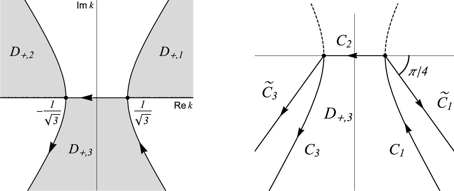
In this section, we first consider the linear KdV equation posed on the quarter plane $\begin{matrix} (4) & u_{t} + u_{x} + u_{x x x} = 0, x > 0, t > 0 . \end{matrix}$ The equation can be written as an overdetermined linear system, known as Lax pair $\begin{array}{l} (5a) & φ_{x} + i k φ = u, \\ (5b) & φ_{t} + i f_{1} (k) φ = i k u_{x} - u_{x x} + (k^{2} - 1) u, \end{array}$ where the dispersion relation is given by $f_{1} (k) = k^{3} - k$ . We introduce the domain $D_{+} = {k \in C ∣ Im f_{1} (k) > 0}$ and we decompose the region $D_{+}$ into $D_{+} = D_{+, 1} \cup D_{+, 2} \cup D_{+, 3}$ (see Fig. 1). Letting the closed differential 1-form $W (x, t, k)$ given by $\begin{matrix} W (x, t, k) = e^{i k x + i f_{1} (k) t} [u d x + (i k u_{x} - u_{x x} + (k^{2} - 1) u) d t], \end{matrix}$ we write the Lax pair (5) as $\begin{matrix} (6) & d (e^{i k x + i f_{1} (k) t} φ) = W (x, t, k) . \end{matrix}$ Employing the Green theorem on $(0, \infty) \times (0, t)$ , we find the global relation for the linear KdV equation $\begin{matrix} (7) & {\hat{u}}_{0} (k) - e^{i f_{1} (k) t} \hat{u} (k, t) + \hat{G} (k, t) = 0, Im k ⩾ 0, \end{matrix}$ where $\begin{array}{l} \hat{u} (k, t) = \int_{0}^{\infty} e^{i k x} u (x, t) d x, Im k ⩾ 0, \\ \hat{G} (k, t) = - i k {\hat{g}}_{1} (k, t) + {\hat{g}}_{2} (k, t) - (k^{2} - 1) {\hat{g}}_{0} (k, t) \end{array}$ with $\begin{matrix} {\hat{g}}_{j} (k, t) = \int_{0}^{t} e^{i f_{1} (k) s} g_{j} (s) d s, j = 0, 1, 2 . \end{matrix}$ Multiplying (7) by $\frac{1}{2 π} e^{- i k x - i f_{1} (k) t}$ and applying the inverse Fourier transform, we find $\begin{matrix} (8) & u (x, t) = \frac{1}{2 π} \int_{- \infty}^{\infty} e^{- i k x - i f_{1} (k) t} {\hat{u}}_{0} (k) d k + \frac{1}{2 π} \int_{- \infty}^{\infty} e^{- i k x - i f_{1} (k) t} \hat{G} (k, t) d k . \end{matrix}$ We deform the contour $(- \infty, \infty)$ to $\partial D_{+, 3}$ for the second integral in (8) and then equation (8) can be expressed as $\begin{matrix} (9) & u (x, t) = \frac{1}{2 π} \int_{- \infty}^{\infty} e^{- i k x - i f_{1} (k) t} {\hat{u}}_{0} (k) d k - \frac{1}{2 π} \int_{\partial D_{+, 3}} e^{- i k x - i f_{1} (k) t} \hat{G} (k, t) d k . \end{matrix}$ Note that the representation of the solution (9) involves the unknown boundary data $u_{x} (0, t)$ and $u_{x x} (0, t)$ via ${\hat{g}}_{j} (k, t)$ , $j = 1, 2$ . Thus, for the explicit representation of the solution, it is necessary to determine these unknown boundary data. To this end, we use the global relation (7).

Note that if $k^{3} - k = ν^{3} - ν$ , the transformation $k \to ν (k)$ leaves $f_{1} (k)$ invariant. As a consequence, ${\hat{g}}_{j} (k, t)$ is invariant under this transformation. The equation $k^{3} - k = ν^{3} - ν$ has a trivial root $ν (k) = k$ and nontrivial roots $\begin{matrix} (10) & ν (k) = \frac{1}{2} (- k + {(3 k^{2} - 4)}^{1 / 2}) . \end{matrix}$ Equation (10) is a double-valued expression and in particular, it has branch points at $k = \pm 2 / \sqrt{3}$ . In order to make (10) single-valued, we define a branch cut along $(- \infty, - 2 / \sqrt{3}] \cup [2 / \sqrt{3}, \infty]$ . Also, we choose $ν (k)$ that satisfies $ν (k) \sim \frac{1}{2} e^{\pm 2 i π / 3} k$ for large k. Thus, we denote these roots by $\begin{matrix} (11) & ν_{1, 2} (k) = \frac{1}{2} (- k \pm i \sqrt{3 k^{2} - 4}) . \end{matrix}$ Note that $ν_{1} (k) \in D_{+, 1}$ and $ν_{2} (k) \in D_{+, 2}$ , respectively, for $k \in D_{+, 3}$ .

Thus, letting $k \to ν_{1} (k)$ and $k \to ν_{2} (k)$ in (7) for $k \in D_{+, 3}$ , we find the following equations $\begin{array}{l} (12a) & {\hat{u}}_{0} (ν_{1} (k)) - (ν_{1}^{2} (k) - 1) {\hat{g}}_{0} (k, t) - e^{i f_{1} (k) t} \hat{u} (ν_{1} (k), t) = i ν_{1} (k) {\hat{g}}_{1} (k, t) - {\hat{g}}_{2} (k, t), \\ (12b) & {\hat{u}}_{0} (ν_{2} (k)) - (ν_{2}^{2} (k) - 1) {\hat{g}}_{0} (k, t) - e^{i f_{1} (k) t} \hat{u} (ν_{2} (k), t) = i ν_{2} (k) {\hat{g}}_{1} (k, t) - {\hat{g}}_{2} (k, t) \end{array}$ and then we solve the linear system (12) for ${\hat{g}}_{1}$ and ${\hat{g}}_{2}$ : $\begin{array}{l} {\hat{g}}_{1} (k, t) = & i (ν_{1} (k) + ν_{2} (k)) {\hat{g}}_{0} (t) + \frac{i}{ν_{1} (k) - ν_{2} (k)} {{\hat{u}}_{0} (ν_{2} (k)) - {\hat{u}}_{0} (ν_{1} (k)) \\ (13a) & + e^{i f_{1} (k) t} [\hat{u} (ν_{1} (k), t) - \hat{u} (ν_{2} (k), t)]}, \\ {\hat{g}}_{2} (k, t) = & - (ν_{1} (k) ν_{2} (k) + 1) {\hat{g}}_{0} (t) + \frac{1}{ν_{1} (k) - ν_{2} (k)} {ν_{2} (k) {\hat{u}}_{0} (ν_{1} (k)) - ν_{1} (k) {\hat{u}}_{0} (ν_{2} (k)) \\ (13b) & + e^{i f_{1} (k) t} [ν_{1} (k) \hat{u} (ν_{2} (k), t) - ν_{2} (k) \hat{u} (ν_{1} (k), t)]} . \end{array}$ Finally, substituting (13) into (9), the solution of (4) is given by $\begin{array}{l} u (x, t) = & \frac{1}{2 π} \int_{- \infty}^{\infty} e^{- i k x - i f_{1} (k) t} {\hat{u}}_{0} (k) d k - \frac{1}{2 π} \int_{\partial D_{+, 3}} e^{- i k x - i f_{1} (k) t} [\frac{k - ν_{1} (k)}{ν_{1} (k) - ν_{2} (k)} {\hat{u}}_{0} (ν_{2} (k)) \\ (14) & - \frac{k - ν_{2} (k)}{ν_{1} (k) - ν_{2} (k)} {\hat{u}}_{0} (ν_{1} (k)) - (3 k^{2} - 1) {\hat{g}}_{0} (k, t)] d k, \end{array}$ where we have used the fact that the terms involving $e^{i f_{1} (k) t}$ in (13) yield a zero contribution to (9) due to the Cauchy theorem.

The representation of the solution given in (14) allows to show that the solution for the linear KdV equation with a periodic Dirichlet boundary datum is asymptotically periodic for large t. The similar result of the Proposition 2.1 also can be found in [22].

Proposition 2.1.
Assume that $u_{0} (x)$ is a function of the Schwartz class, denoted by $S [0, \infty)$ and $g_{0} (t) \in L^{\infty} [0, \infty)$ , where $g_{0} (t)$ is a periodic function with period τ. Let $u (x, t)$ be the solution given by ( 14 ). Then for any $x > 0$ , $\begin{matrix} (15) & lim_{n \to \infty} u (x, n τ + t) = u_{\infty} (x, t), \end{matrix}$ where $u_{\infty} (x, t)$ is a periodic function with period τ and $u_{\infty} (0, t) = g_{0} (t)$ . In particular, for any $x > 0$ , $u (x, t)$ is asymptotically periodic in the sense that $\begin{matrix} (16) & u (x, τ + t) - u (x, t) = O (t^{- 1 / 2}), t \to \infty . \end{matrix}$
Proof.
We write $u (x, t)$ given in (14) as $u (x, t) = U^{(1)} (x, t) + U^{(2)} (x, t) + U^{(3)} (x, t)$ , where $\begin{array}{l} (17a) & U^{(1)} (x, t) = \frac{1}{2 π} \int_{- \infty}^{\infty} e^{- i k x - i f_{1} (k) t} {\hat{u}}_{0} (k) d k, \\ (17b) & U^{(2)} (x, t) = - \frac{1}{2 π} \int_{\partial D_{+, 3}} e^{- i k x - i f_{1} (k) t} [\frac{(k - ν_{1} (k)) {\hat{u}}_{0} (ν_{2} (k))}{ν_{1} (k) - ν_{2} (k)} - \frac{(k - ν_{2} (k)) {\hat{u}}_{0} (ν_{1} (k))}{ν_{1} (k) - ν_{2} (k)}] d k, \\ (17c) & U^{(3)} (x, t) = \frac{1}{2 π} \int_{\partial D_{+, 3}} e^{- i k x - i f_{1} (k) t} (3 k^{2} - 1) {\hat{g}}_{0} (k, t) d k . \end{array}$ We will evaluate each integral in (17) for large t in order to show (15). For $U^{(1)} (x, t)$ , we write $\begin{matrix} U^{(1)} (x, t) = \frac{1}{2 π} \int_{0}^{\infty} u_{0} (y) \int_{- \infty}^{\infty} e^{- i k (x - y) - i f_{1} (k) t} d k d y \end{matrix}$ and then we consider the following integral $\begin{matrix} (18) & \int_{- \infty}^{\infty} e^{- i k (x - y) - i f_{1} (k) t} d k . \end{matrix}$ Note that $- i f_{1} (k)$ has critical points at $k = \pm 1 / \sqrt{3}$ and $e^{- i k (x - y)} = e^{\mp i (x - y) / \sqrt{3}} + O (k \pm 1 / \sqrt{3})$ as $k \to \pm 1 / \sqrt{3}$ . Thus, we introduce the steepest descent contours ${\tilde{C}}_{1}$ and ${\tilde{C}}_{3}$ , where ${\tilde{C}}_{1}$ and ${\tilde{C}}_{3}$ are the rays starting at $k = \pm 1 / \sqrt{3}$ with directions $- π / 4$ and $5 π / 4$ , respectively (see Fig. 1). Deforming the contour $(- \infty, \infty)$ to the contour ${\tilde{C}}_{1} - C_{2} - {\tilde{C}}_{3}$ , we know that $\begin{matrix} (19) & \int_{- \infty}^{\infty} e^{- i k (x - y) - i f_{1} (k) t} d k \sim \int_{{\tilde{C}}_{1} - C_{2} - {\tilde{C}}_{3}} e^{- i k (x - y) - i f_{1} (k) t} d k, t \to \infty, \end{matrix}$ where the contour $C_{2}$ is given by $- C_{2} = [- 1 / \sqrt{3}, 1 / \sqrt{3}]$ (cf. Fig. 1). Using the steepest descent method along the contour ${\tilde{C}}_{1} - {\tilde{C}}_{3}$ and applying the stationary phase method along the contour $C_{2}$ , respectively, we find $\begin{matrix} \int_{- \infty}^{\infty} e^{- i k (x - y) - i f_{1} (k) t} d k = O (t^{- 1 / 2}), t \to \infty . \end{matrix}$ Thus, the following estimate for $U^{(1)} (x, t)$ can be derived $\begin{matrix} (20) & | U^{(1)} (x, t) | ⩽ \frac{M_{1}}{\sqrt{t}} ‖ u_{0} ‖_{L^{1} [0, \infty)} \end{matrix}$ for some constant $M_{1} > 0$ .

For $U^{(2)} (x, t)$ , we first consider the integral $\begin{array}{l} \frac{1}{2 π} \int_{\partial D_{+, 3}} e^{- i k x - i f_{1} (k) t} \frac{(k - ν_{1} (k)) {\hat{u}}_{0} (ν_{2} (k))}{ν_{1} (k) - ν_{2} (k)} d k \\ (21) & = \frac{1}{2 π} \int_{0}^{\infty} u_{0} (y) \int_{\partial D_{+, 3}} e^{- i (k x - ν_{2} (k) y) - i f_{1} (k) t} \frac{k - ν_{1} (k)}{ν_{1} (k) - ν_{2} (k)} d k d y . \end{array}$ Note that $\begin{array}{l} e^{- i (k x - ν_{2} (k) y)} \frac{k - ν_{1} (k)}{ν_{1} (k) - ν_{2} (k)} = \{\begin{matrix} - e^{- i (x - y) / \sqrt{3}} + O (k - 1 / \sqrt{3}), & k \to 1 / \sqrt{3}, \\ O (k + 1 / \sqrt{3}), & k \to - 1 / \sqrt{3} . \end{matrix} \end{array}$ Thus, using the steepest descent and stationary phase methods for the integral with respect to k in (21), we find the asymptotic evaluation $\begin{matrix} (22) & \int_{\partial D_{+, 3}} e^{- i (k x - ν_{2} (k) y) - i f_{1} (k) t} \frac{k - ν_{1} (k)}{ν_{1} (k) - ν_{2} (k)} d k = O (t^{- 1 / 2}), t \to \infty . \end{matrix}$ A similar asymptotic analysis is also valid for the second integral in (17b), and hence the estimate for $U^{(2)} (x, t)$ can be obtained as $\begin{matrix} (23) & | U^{(2)} (x, t) | ⩽ \frac{M_{2}}{\sqrt{t}} ‖ u_{0} ‖_{L^{1} [0, \infty)} \end{matrix}$ for some constant $M_{2} > 0$ .

Regarding $U^{(3)} (x, t)$ , note that by integration by parts, $(3 k^{2} - 1) {\hat{g}}_{0} (k, t) = O (1 / k)$ as $k \to \infty$ . Hence, by the Cauchy theorem, we deform the contour $\partial D_{+, 3}$ to $(- \infty, \infty)$ and then we write $U^{(3)} (x, t)$ as $\begin{matrix} (24) & U^{(3)} (x, t) = - \frac{1}{2 π} \int_{0}^{t} g_{0} (s) Φ (x, t - s) d s, \end{matrix}$ where $\begin{matrix} (25) & Φ (x, t) = \int_{- \infty}^{\infty} e^{- i k x - i f_{1} (k) t} (3 k^{2} - 1) d k . \end{matrix}$ Note that since $f_{1}^{'} (k) = 3 k^{2} - 1$ , $\begin{matrix} Φ (x, t) = - \frac{1}{i t} \int_{- \infty}^{\infty} e^{- i k x} \frac{d}{d k} (e^{- i f_{1} (k) t}) d k = - \frac{x}{t} \int_{- \infty}^{\infty} e^{- i k x - i f_{1} (k) t} d k . \end{matrix}$ As before, the steepest descent and stationary phase methods yield that $Φ (x, t) = O (t^{- 3 / 2})$ as $t \to \infty$ .

We now prove (15). In this respect, let ${u_{n} (x, t)}_{1}^{\infty}$ be the sequence given by $\begin{matrix} (26) & u_{n} (x, t) = u (x, n τ + t) = U_{n}^{(1)} (x, t) + U_{n}^{(2)} (x, t) + U_{n}^{(3)} (x, t), \end{matrix}$ where $U_{n}^{(j)} (x, t) = U^{(j)} (x, n τ + t)$ for $j = 1, 2, 3$ . From (20) and (23), it follows that $\begin{matrix} | U_{n}^{(1)} (x, t) + U_{n}^{(2)} (x, t) | ⩽ \frac{M_{1} + M_{2}}{\sqrt{n τ + t}} ‖ u_{0} ‖_{L^{1} [0, \infty)}, \end{matrix}$ which implies that $\begin{matrix} (27) & lim_{n \to \infty} [U_{n}^{(1)} (x, t) + U_{n}^{(2)} (x, t)] = 0 . \end{matrix}$ For $U_{n}^{(3)} (x, t)$ , consider the following series $\begin{matrix} (28) & \sum_{m = 1}^{\infty} [U_{m + 1}^{(3)} (x, t) - U_{m}^{(3)} (x, t)] . \end{matrix}$ Since $g_{0} (t)$ is periodic, we know that $\begin{matrix} U_{m + 1}^{(3)} (x, t) - U_{m}^{(3)} (x, t) = \frac{1}{2 π} \int_{m τ + t}^{(m + 1) τ + t} g_{0} (t - s) Φ (x, s) d s . \end{matrix}$ Then, since $Φ (x, t) = O (t^{- 3 / 2})$ as $t \to \infty$ , we find the following estimate $\begin{matrix} (29) & | U_{m + 1}^{(3)} (x, t) - U_{m}^{(3)} (x, t) | ⩽ \frac{M_{3}}{{(m τ + t)}^{3 / 2}} ‖ g_{0} ‖_{L^{\infty} [0, \infty)} \end{matrix}$ for some constant $M_{3} > 0$ . Thus, the series given in (28) converges and so does the sequence $U_{n}^{(3)} (x, t)$ as $n \to \infty$ . As a consequence, the limit of the sequence ${u_{n} (x, t)}$ given in (26) exists for any $x > 0$ and this limit, denoted by $u_{\infty} (x, t)$ , is a periodic function with period τ. Indeed, note that $\begin{array}{l} u_{\infty} (x, τ + t) - u_{\infty} (x, t) = [u_{\infty} (x, τ + t) - u_{n} (x, τ + t)] + [u_{n + 1} (x, t) - u_{\infty} (x, t)] . \end{array}$ Taking $n \to \infty$ , we find $u_{\infty} (x, τ + t) = u_{\infty} (x, t)$ . Moreover, $u_{n} (0, t) = g_{0} (t)$ implies $u_{\infty} (0, t) = g_{0} (t)$ . □

Next, we study the asymptotically periodic boundary data for large t. We note that by integration by parts, the function ${\hat{g}}_{0} (k, t)$ can be written as $\begin{matrix} {\hat{g}}_{0} (k, t) = \frac{1}{i f_{1} (k)} (e^{i f_{1} (k) t} g_{0} (t) - g_{0} (0)) - \frac{1}{i f_{1} (k)} \int_{0}^{t} e^{i f_{1} (k) s} {\dot{g}}_{0} (s) d s . \end{matrix}$ Deforming the contour $\partial D_{+, 3}$ to pass to the right of the singularity $k = 0$ , which is denoted by $\partial D_{+, 3}^{0}$ , equation (14) can be expressed as $\begin{array}{l} u (x, t) = & \frac{1}{2 π} \int_{- \infty}^{\infty} e^{- i k x - i f_{1} (k) t} {\hat{u}}_{0} (k) d k \\ - \frac{1}{2 π} \int_{\partial D_{+, 3}} e^{- i k x - i f_{1} (k) t} [\frac{k - ν_{1} (k)}{ν_{1} (k) - ν_{2} (k)} {\hat{u}}_{0} (ν_{2} (k)) \\ - \frac{k - ν_{2} (k)}{ν_{1} (k) - ν_{2} (k)} {\hat{u}}_{0} (ν_{1} (k))] d k + g_{0} (t) \\ (30) & - \frac{1}{2 i π} \int_{\partial D_{+, 3}^{0}} e^{- i k x - i f_{1} (k) t} \frac{(3 k^{2} - 1)}{f_{1} (k)} [g_{0} (0) + \int_{0}^{t} e^{i f_{1} (k) s} {\dot{g}}_{0} (s) d s] d k . \end{array}$ Differentiating (30) with respect to x and evaluating at $x = 0$ , we find $g_{1} (t)$ given by $\begin{array}{l} g_{1} (t) = & \frac{1}{2 i π} \int_{- \infty}^{\infty} k e^{- i f_{1} (k) t} {\hat{u}}_{0} (k) d k - \frac{1}{2 i π} \int_{\partial D_{+, 3}} k e^{- i f_{1} (k) t} [\frac{k - ν_{1} (k)}{ν_{1} (k) - ν_{2} (k)} {\hat{u}}_{0} (ν_{2} (k)) \\ - \frac{k - ν_{2} (k)}{ν_{1} (k) - ν_{2} (k)} {\hat{u}}_{0} (ν_{1} (k))] d k \\ (31) & + \frac{1}{2 π} \int_{\partial D_{+, 3}} e^{- i f_{1} (k) t} \frac{k (3 k^{2} - 1)}{f_{1} (k)} [g_{0} (0) + \int_{0}^{t} e^{i f_{1} (k) s} {\dot{g}}_{0} (s) d s] d k . \end{array}$ Similarly, $g_{2} (t)$ is given by $\begin{array}{l} g_{2} (t) = & - \frac{1}{2 π} \int_{- \infty}^{\infty} k^{2} e^{- i f_{1} (k) t} {\hat{u}}_{0} (k) d k + \frac{1}{2 π} \int_{\partial D_{+, 3}} k^{2} e^{- i f_{1} (k) t} [\frac{k - ν_{1} (k)}{ν_{1} (k) - ν_{2} (k)} {\hat{u}}_{0} (ν_{2} (k)) \\ - \frac{k - ν_{2} (k)}{ν_{1} (k) - ν_{2} (k)} {\hat{u}}_{0} (ν_{1} (k))] d k \\ (32) & + \frac{1}{2 i π} \int_{\partial D_{+, 3}} e^{- i f_{1} (k) t} \frac{k^{2} (3 k^{2} - 1)}{f_{1} (k)} [g_{0} (0) + \int_{0}^{t} e^{i f_{1} (k) s} {\dot{g}}_{0} (s) d s] d k . \end{array}$ Proposition 2.2.
Let ${\tilde{g}}_{0} (t)$ be a smooth periodic function with period $τ = 2 π$ . Assume that ${\tilde{g}}_{0} (t)$ has the Fourier series $\begin{matrix} (33) & {\tilde{g}}_{0} (t) = \sum_{n = - \infty}^{\infty} a_{n} e^{i n t}, t ⩾ 0, \end{matrix}$ where $a_{n} \in C$ with $a_{0} = 0$ . Then, there are unique periodic functions ${\tilde{g}}_{1} (t)$ and ${\tilde{g}}_{2} (t)$ such that $u (0, \cdot) - {\tilde{g}}_{0} \in S [0, \infty)$ and $\begin{matrix} (34) & u_{x} (0, t) - {\tilde{g}}_{1} (t) = O (t^{- 1 / 2}), u_{x x} (0, t) - {\tilde{g}}_{2} (t) = O (t^{- 1 / 2}), t \to \infty . \end{matrix}$ Moreover, the functions ${\tilde{g}}_{1} (t)$ and ${\tilde{g}}_{2} (t)$ have period τ and the Fourier series are given by $\begin{matrix} (35) & {\tilde{g}}_{1} (t) = \sum_{n = - \infty}^{\infty} (- i k_{n} a_{n}) e^{i n t}, {\tilde{g}}_{2} (t) = \sum_{n = - \infty}^{\infty} (- k_{n}^{2} a_{n}) e^{i n t}, \end{matrix}$ where $\begin{matrix} (36) & k_{n} = \{\begin{matrix} \frac{1}{\sqrt[3]{36} K (n)} (2 \sqrt[3]{3} e^{- i π / 3} + \sqrt[3]{2} K^{2} (n) e^{i π / 3}), & n > 0, \\ \frac{1}{\sqrt[3]{36} K (- n)} (2 \sqrt[3]{3} e^{- 2 i π / 3} + \sqrt[3]{2} K^{2} (- n) e^{2 i π / 3}), & n < 0 \end{matrix} \end{matrix}$ with $K (n) = \sqrt[3]{9 n - \sqrt{81 n^{2} - 12}}$ .
Proof.
Let $u (x, t)$ be the solution given in (30) with $g_{0} (t) = {\tilde{g}}_{0} (t)$ . We first prove that $g_{1} (t) - {\tilde{g}}_{1} (t) = O (t^{- 1 / 2})$ as $t \to \infty$ . We write (31) as $g_{1} (t) = I_{1} (t) + I_{2} (t) + I_{3} (t)$ , where $\begin{array}{l} (37a) & I_{1} (t) = \frac{1}{2 i π} \int_{- \infty}^{\infty} k e^{- i f_{1} (k) t} {\hat{u}}_{0} (k) d k, \\ (37b) & I_{2} (t) = - \frac{1}{2 i π} \int_{\partial D_{+, 3}} k e^{- i f_{1} (k) t} [\frac{k - ν_{1} (k)}{ν_{1} (k) - ν_{2} (k)} {\hat{u}}_{0} (ν_{2} (k)) - \frac{k - ν_{2} (k)}{ν_{1} (k) - ν_{2} (k)} {\hat{u}}_{0} (ν_{1} (k))] d k, \\ (37c) & I_{3} (t) = \frac{1}{2 π} \int_{\partial D_{+, 3}} e^{- i f_{1} (k) t} \frac{k (3 k^{2} - 1)}{f_{1} (k)} [g_{0} (0) + \int_{0}^{t} e^{i f_{1} (k) s} {\dot{g}}_{0} (s) d s] d k . \end{array}$ Note that using Integration by parts, we find $\begin{array}{l} I_{1} (t) = & \frac{1}{2 π} \int_{- \infty}^{\infty} e^{- i f_{1} (k) t} u_{0} (0) d k + \frac{1}{2 π} \int_{- \infty}^{\infty} e^{- i f_{1} (k) t} \int_{0}^{\infty} e^{i k x} {\dot{u}}_{0} (x) d x d k \end{array}$ and hence, from the equations $\begin{matrix} \frac{1}{2 π} \int_{- \infty}^{\infty} e^{- i f_{1} (k) t} d k = \frac{1}{\sqrt[3]{3 t}} Ai (- \frac{t^{2 / 3}}{\sqrt[3]{3}}), \frac{1}{2 π} \int_{- \infty}^{\infty} e^{i k x - i f_{1} (k) t} d k = \frac{1}{\sqrt[3]{3 t}} Ai (- \frac{t + x}{\sqrt[3]{3 t}}), \end{matrix}$ it immediately follows that $I_{1} (t) = O (t^{- 1 / 2})$ as $t \to \infty$ , where $Ai (s)$ is the Airy function.

For the integral $I_{2} (t)$ , we consider the following integral $\begin{matrix} (38) & \int_{\partial D_{+, 3}} e^{i ν_{2} (k) x - i f_{1} (k) t} \frac{k (k - ν_{1} (k))}{ν_{1} (k) - ν_{2} (k)} d k . \end{matrix}$ The asymptotic evaluation for the integral (38) is similar to the proof of Proposition 2.1. We first decompose the contour $\partial D_{+, 3}$ into $\partial D_{+, 3} = C_{1} + C_{2} + C_{3}$ , where the contours $C_{1}$ , $C_{2}$ and $C_{3}$ are depicted in Fig. 1. Then we deform the contour $C_{1}$ and $C_{3}$ to the steepest descent contours $- {\tilde{C}}_{1}$ and ${\tilde{C}}_{3}$ , respectively (cf. Fig. 1). Note that $\begin{array}{l} e^{i ν_{2} (k) x} \frac{k (k - ν_{1} (k))}{ν_{1} (k) - ν_{2} (k)} = \{\begin{matrix} - \frac{e^{i x / \sqrt{3}}}{\sqrt{3}} + O (k - 1 / \sqrt{3}), & k \to 1 / \sqrt{3}, \\ O (k + 1 / \sqrt{3}), & k \to - 1 / \sqrt{3} . \end{matrix} \end{array}$ Thus, using the steepest descent method, we find that the integral along the contour $- {\tilde{C}}_{1} + {\tilde{C}}_{3}$ in (38) is of $O (t^{- 1 / 2})$ as $t \to \infty$ , that is, $\begin{matrix} (39) & \int_{- {\tilde{C}}_{1} + {\tilde{C}}_{3}} e^{i ν_{2} (k) x - i f_{1} (k) t} \frac{k (k - ν_{1} (k))}{ν_{1} (k) - ν_{2} (k)} d k = O (t^{- 1 / 2}), t \to \infty . \end{matrix}$ The integral along the contour $C_{2}$ in (38) can be evaluated by using the stationary phase method and it is of $O (t^{- 1 / 2})$ as $t \to \infty$ . Thus, we find $\begin{array}{l} \int_{\partial D_{+, 3}} k e^{- i f_{1} (k) t} \frac{k - ν_{1} (k)}{ν_{1} (k) - ν_{2} (k)} {\hat{u}}_{0} (ν_{2} (k)) d k \\ = \int_{0}^{\infty} u_{0} (x) \int_{\partial D_{+, 3}} e^{i ν_{2} (k) x - i f_{1} (k) t} \frac{k (k - ν_{1} (k))}{ν_{1} (k) - ν_{2} (k)} d k d x = O (t^{- 1 / 2}), t \to \infty . \end{array}$ In similar ways, we evaluate $\begin{matrix} \int_{\partial D_{+, 3}} k e^{- i f_{1} (k) t} \frac{k - ν_{2} (k)}{ν_{1} (k) - ν_{2} (k)} {\hat{u}}_{0} (ν_{1} (k)) d k = O (t^{- 1 / 2}), t \to \infty \end{matrix}$ and hence $I_{2} (t) = O (t^{- 1 / 2})$ as $t \to \infty$ .

Regarding the integral $I_{3} (t)$ , integration by parts yields $\begin{matrix} (40) & I_{3} (t) = \frac{1}{2 π} \int_{\partial D_{+, 3}} [\frac{k (3 k^{2} - 1)}{f_{1} (k)} g_{0} (t) - i k (3 k^{2} - 1) \int_{0}^{t} e^{- i (t - s) f_{1} (k)} g_{0} (s) d s] d k . \end{matrix}$ Substituting the Fourier expansion (33) into the above equation, we find $\begin{array}{l} I_{3} (t) & = \frac{1}{2 π} \int_{\partial D_{+, 3}} k (3 k^{2} - 1) \sum_{n \neq 0} a_{n} (\frac{e^{i n t}}{f_{1} (k)} - i \int_{0}^{t} e^{i n s - i (t - s) f_{1} (k)} d s) d k \\ (41) & = \frac{1}{2 π} \int_{\partial D_{+, 3}} k (3 k^{2} - 1) \sum_{n \neq 0} a_{n} (\frac{e^{i n t}}{f_{1} (k)} - \frac{e^{i n t} - e^{- i f_{1} (k) t}}{f_{1} (k) + n}) d k . \end{array}$ For each $n \in Z$ , $k_{n}$ given in (36) solves the equation $f_{1} (k) + n = 0$ in $\partial D_{+, 3}$ . Thus, we deform the contour $\partial D_{+, 3}$ to passe to the right of the singularities $k = k_{n}$ , which is denoted by $\partial {\hat{D}}_{+, 3}$ , before we split the integral (41). As a result, we find $\begin{array}{l} I_{3} (t) = & \frac{1}{2 π} \sum_{n \neq 0} a_{n} e^{i n t} \int_{\partial {\hat{D}}_{+, 3}} k (3 k^{2} - 1) (\frac{1}{f_{1} (k)} - \frac{1}{f_{1} (k) + n}) d k \\ (42) & + \frac{1}{2 π} \int_{\partial {\hat{D}}_{+, 3}} k (3 k^{2} - 1) e^{- i f_{1} (k) t} \sum_{n \neq 0} (\frac{a_{n}}{f_{1} (k) + n}) d k . \end{array}$ The first integral in (42) can be evaluated by the residue theorem: $\begin{array}{l} \frac{1}{2 π} \sum_{n \neq 0} a_{n} e^{i n t} \int_{\partial {\hat{D}}_{+, 3}} k (3 k^{2} - 1) (\frac{1}{f_{1} (k)} - \frac{1}{f_{1} (k) + n}) d k = - i \sum_{n \neq 0} k_{n} a_{n} e^{i n t} = {\tilde{g}}_{1} (t) . \end{array}$ For the second integral in (42), we deform $\partial {\hat{D}}_{+, 3}$ to the steepest descent contour $- {\tilde{C}}_{1} + C_{2} + {\tilde{C}}_{3}$ and then the steepest descent and the stationary phase methods yield $\begin{matrix} \frac{1}{2 π} \int_{\partial {\hat{D}}_{+, 3}} k (3 k^{2} - 1) e^{- i f_{1} (k) t} \sum_{n \neq 0} (\frac{a_{n}}{f_{1} (k) + n}) d k = O (t^{- 1 / 2}), t \to \infty . \end{matrix}$ Thus, $g_{1} (t) = {\tilde{g}}_{1} (t) + O (t^{- 1 / 2})$ as $t \to \infty$ .

In similar ways, we can prove that $g_{2} (t) = {\tilde{g}}_{2} (t) + O (t^{- 1 / 2})$ as $t \to \infty$ where $g_{2} (t)$ and ${\tilde{g}}_{2} (t)$ are given by (32) and the second equation of (35), respectively. Also, the uniqueness of ${\tilde{g}}_{1} (t)$ and ${\tilde{g}}_{2} (t)$ follows from the fact that $u (0, \cdot) - {\tilde{g}}_{0} (t) \in S [0, \infty)$ (see [21] for some details). □

3. The KdV equation

3.1. Eigenfunctions

In this section, we study the KdV equation posed on the quarter plane $\begin{matrix} (43) & u_{t} + u_{x} + u_{x x x} + 6 u u_{x} = 0, x > 0, t > 0 . \end{matrix}$ We assume that $u_{0} (x) = u (x, 0)$ and $g_{0} (t) = u (0, t)$ are given, while $g_{1} (t) = u_{x} (0, t)$ and $g_{2} (t) = u_{x x} (0, t)$ are unknown. It is known that (43) admits a Lax pair formulation of the form $\begin{array}{l} (44a) & μ_{x} + i k {\hat{σ}}_{3} μ = U (x, t) μ, \\ (44b) & μ_{t} + i f_{2} (k) {\hat{σ}}_{3} μ = V (x, t, k) μ, \end{array}$ where $k \in C$ is a spectral parameter, $μ (x, t, k)$ is a $2 \times 2$ matrix-valued eigenfunction and $\begin{array}{l} (45) & f_{2} (k) = 4 k^{3} - k, {\hat{σ}}_{3} A = σ_{3} A - A σ_{3}, U (x, t) = \frac{u}{2 k} (σ_{2} - i σ_{3}), \\ (46) & V (x, t, k) = 2 k u σ_{2} + u_{x} σ_{1} + \frac{2 u^{2} + u + u_{x x}}{2 k} (i σ_{3} - σ_{2}) \end{array}$ with the usual Pauli matrices $σ_{j}$ defined by $\begin{matrix} σ_{1} = (\begin{matrix} 0 & 1 \\ 1 & 0 \end{matrix}), σ_{2} = (\begin{matrix} 0 & - i \\ i & 0 \end{matrix}), σ_{3} = (\begin{matrix} 1 & 0 \\ 0 & - 1 \end{matrix}) . \end{matrix}$ Letting the closed differential 1-form given by $\begin{matrix} (47) & W_{j} (x, t, k) = [U d x + V d t] μ_{j} (x, t, k), j = 2, 3, \end{matrix}$ we define the normalized solutions of (44) at $(x_{2}, t_{2}) = (0, 0)$ and $(x_{3}, t_{3}) = (\infty, t)$ in terms of the linear Volterra integral equations: $\begin{matrix} (48) & μ_{j} (x, t, k) = I + \int_{(x_{j}, t_{j})}^{(x, t)} e^{i (k (x^{'} - x) + f_{2} (k) (t^{'} - t)) {\hat{σ}}_{3}} W_{j} (x^{'}, t^{'}, k), j = 2, 3 . \end{matrix}$ We introduce the domain $\begin{matrix} {\tilde{D}}_{+} = {k \in C ∣ Im f_{2} (k) > 0}, \end{matrix}$ which will also be convenient to decompose as ${\tilde{D}}_{+} = {\tilde{D}}_{+, 1} \cup {\tilde{D}}_{+, 2} \cup {\tilde{D}}_{+, 3}$ , where ${\tilde{D}}_{+, 1} = {\tilde{D}}_{+} \cap C_{I}$ , ${\tilde{D}}_{+, 2} = {\tilde{D}}_{+} \cap C_{II}$ and ${\tilde{D}}_{+, 3} = {\tilde{D}}_{+} \cap {k \in C ∣ Im k < 0}$ with the first and second quadrants $C_{I}$ and $C_{II}$ of the complex k-plane (cf. Fig. 1). Note that the regions $D_{+}$ and ${\tilde{D}}_{+}$ are similar, but the hyperbolas for the linear and nonlinear cases are slightly different.

In order to define an additional eigenfunction $μ_{1} (x, t, k)$ , let $\tilde{ψ} (t, k)$ be the solution of the background t-part of the Lax pair with the asymptotically periodic boundary data $\begin{matrix} (49) & {\tilde{ψ}}_{t} + i f_{2} (k) σ_{3} \tilde{ψ} = \tilde{V} \tilde{ψ}, \end{matrix}$ where $\tilde{V} (t, k)$ is the matrix-valued function defined by replacing $u (0, t)$ , $u_{x} (0, t)$ and $u_{x x} (0, t)$ by ${\tilde{g}}_{0} (t)$ , ${\tilde{g}}_{1} (t)$ and ${\tilde{g}}_{2} (t)$ , respectively. More specifically, we denote $\tilde{V} (t, k)$ as $\begin{matrix} (50) & \tilde{V} (t, k) = (\begin{matrix} {\tilde{V}}_{1} (t, k) & {\tilde{V}}_{2} (t, - k) \\ {\tilde{V}}_{2} (t, k) & {\tilde{V}}_{1} (t, - k) \end{matrix}), \end{matrix}$ where $\begin{array}{l} {\tilde{V}}_{1} (t, k) = \frac{i}{2 k} (2 {\tilde{g}}_{0}^{2} (t) + {\tilde{g}}_{0} (t) + {\tilde{g}}_{2} (t)), \\ {\tilde{V}}_{2} (t, k) = 2 i k {\tilde{g}}_{0} (t) + {\tilde{g}}_{1} (t) + \frac{1}{2 i k} (2 {\tilde{g}}_{0}^{2} (t) + {\tilde{g}}_{0} (t) + {\tilde{g}}_{2} (t)) . \end{array}$ We seek a solution of (49) in the form of $\tilde{ψ} (t, k) = E (t, k) e^{- i Ω (k) t σ_{3}}$ , where $E (t, k)$ is a periodic function with period τ and $Ω (k)$ is a complex-valued function. Then, the solution $μ_{1} (x, t, k)$ can be defined by $\begin{array}{l} μ_{1} (x, t, k) = & e^{- i k x {\hat{σ}}_{3}} {E (t, k) + \int_{0}^{x} e^{i k x^{'} {\hat{σ}}_{3}} [U (x^{'}, t) μ_{1} (x^{'} t, k)] d x^{'} \\ (51) & - E (t, k) \int_{t}^{\infty} e^{i Ω (k) (t^{'} - t) {\hat{σ}}_{3}} [E^{- 1} (V_{0} - \tilde{V}) (t^{'}, k) μ_{1} (0, t^{'}, k)] d t^{'}}, \end{array}$ where $V_{0} (t, k) = V (0, t, k)$ . From the exponential terms in (51), the domains ${D_{j}}_{1}^{4}$ are denoted by $\begin{array}{l} D_{1} = {Im k > 0, Im Ω (k) > 0}, D_{2} = {Im k > 0, Im Ω (k) < 0}, \\ D_{3} = {Im k < 0, Im Ω (k) > 0}, D_{4} = {Im k < 0, Im Ω (k) < 0} . \end{array}$

The functions $E (t, k)$ and $Ω (k)$ are defined as follows (see [20] for some details). Assume that $ψ (t, k)$ is a solution of the background t-part (49), which is normalized by $ψ (0, k) = I$ . Let $M (k) = ψ (τ, k)$ be the $2 \times 2$ monodromy matrix. Then $ρ (k)$ and $ρ {(k)}^{- 1}$ are the eigenvalues of $M (k)$ , where $\begin{matrix} ρ (k) = \frac{1}{2} (tr M (k) - \sqrt{Δ (k)}), Δ (k) = {(tr M (k))}^{2} - 4 . \end{matrix}$ Let $P$ be the set of branch points defined by $P = {k \in C ∣ Δ (k) = 0, or M_{12} (k) = 0, or M_{21} (k) = 0}$ and $C$ be a branch cut connecting all points in $P$ . By the Floquet theory, the periodic function $E (t, k)$ is defined by $\begin{matrix} E (t, k) = ψ (t, k) e^{- t B (k)} \tilde{S} (k), k \in C ∖ C, \end{matrix}$ where $\tilde{S} (k)$ is the matrix consisting of the eigenvectors corresponding the eigenvalues of $M (k)$ with $det \tilde{S} (k) = 1$ and the $2 \times 2$ matrix $B (k)$ is given by $B (k) = τ^{- 1} log M (k)$ for $k \in C ∖ C$ . Then the function $\tilde{ψ} (t, k)$ in the form of $\tilde{ψ} (t, k) = E (t, k) e^{- i Ω (k) t σ_{3}}$ for $k \in C ∖ C$ is the solution of (49), where $Ω (k) = i τ^{- 1} log ρ (k)$ .

3.2. Perturbative expansions

We assume that the solution of (43) has a formal power series in a small $ϵ > 0$ : $\begin{matrix} (52) & u (x, t) = \sum_{N = 1}^{\infty} ϵ^{N} u^{(N)} (x, t) \end{matrix}$ and then we substitute this expansion into (43). At each order in the perturbative expansion, we find $\begin{array}{l} O (ϵ) : u_{t}^{(1)} + u_{x}^{(1)} + u_{x x x}^{(1)} = 0, \\ O (ϵ^{2}) : u_{t}^{(2)} + u_{x}^{(2)} + u_{x x x}^{(2)} + 6 u^{(1)} u_{x}^{(1)} = 0, \\ O (ϵ^{3}) : u_{t}^{(3)} + u_{x}^{(3)} + u_{x x x}^{(3)} + 6 (u^{(1)} u_{x}^{(2)} + u^{(2)} u_{x}^{(1)}) = 0, \\ O (ϵ^{4}) : u_{t}^{(4)} + u_{x}^{(4)} + u_{x x x}^{(4)} + 6 (u^{(1)} u_{x}^{(3)} + u^{(2)} u_{x}^{(2)} + u^{(3)} u_{x}^{(1)}) = 0, \dots, \\ O (ϵ^{N}) : u_{t}^{(N)} + u_{x}^{(N)} + u_{x x x}^{(N)} + 6 {u u_{x}}_{N} = 0, \dots, \end{array}$ where ${\dots}_{N}$ denotes the coefficient of $ϵ^{N}$ . We also expand the t-periodic asymptotic boundary data in a formal power series in ϵ: $\begin{matrix} (53) & {\tilde{g}}_{j} (t) = \sum_{N = 1}^{\infty} ϵ^{N} {\tilde{g}}_{j}^{(N)} (t), j = 0, 1, 2 . \end{matrix}$

Proposition 3.1.

Assume that ${{\tilde{g}}_{j}^{(N)} (t)}_{j = 0}^{2}$ are smooth periodic functions with period $τ = 2 π$ and ${u^{(N)} (x, t)}_{1}^{\infty}$ is a perturbative solution for the KdV ( 43 ) such that for each $N ⩾ 1$ , $u^{(N)} (\cdot, t) \in L^{1} [0, \infty)$ and $\begin{matrix} (54) & g_{j}^{(N)} (t) - {\tilde{g}}_{j}^{(N)} (t) = O (t^{- 7 / 2}), t \to \infty, j = 0, 1, 2, \end{matrix}$ where $g_{0}^{(N)} (t) = u^{(N)} (0, t)$ , $g_{1}^{(N)} (t) = u_{x}^{(N)} (0, t)$ and $g_{2}^{(N)} (t) = u_{x x}^{(N)} (0, t)$ for $N ⩾ 1$ . Assume that the function ${\tilde{g}}_{0}^{(N)} (t)$ has the following Fourier series $\begin{matrix} (55) & {\tilde{g}}_{0}^{(N)} (t) = \sum_{n = - \infty}^{\infty} a_{n}^{(N)} e^{i n t}, N ⩾ 1 . \end{matrix}$ Then the Fourier coefficients of $\begin{matrix} (56) & {\tilde{g}}_{1}^{(N)} (t) = \sum_{n = - \infty}^{\infty} b_{n}^{(N)} e^{i n t}, {\tilde{g}}_{2}^{(N)} (t) = \sum_{n = - \infty}^{\infty} c_{n}^{(N)} e^{i n t}, N ⩾ 1, \end{matrix}$ are given by $\begin{array}{l} (57) & b_{n}^{(N)} = \frac{1}{κ_{n} - ω_{1} (κ_{n})} {κ_{n} F_{n} (κ_{n}) - ω_{1} (κ_{n}) F_{n} (ω_{1} (κ_{n}))}_{N} + 2 i (κ_{n} + ω_{1} (κ_{n})) a_{n}^{(N)}, \\ (58) & c_{n}^{(N)} = \frac{2 i κ_{n} ω_{1} (κ_{n})}{κ_{n} - ω_{1} (κ_{n})} {F_{n} (κ_{n}) - F_{n} (ω_{1} (κ_{n}))}_{N} - (4 κ_{n} ω_{1} (κ_{n}) + 1) a_{n}^{(N)}, \end{array}$ where $ω_{1} (k) = \frac{1}{2} (- k + i \sqrt{3 k^{2} - 1})$ for $k \in {\bar{\tilde{D}}}_{+, 1}$ , $\begin{array}{l} (59) & κ_{n} = \{\begin{matrix} \frac{1}{2 \sqrt[3]{9} K (n)} (\sqrt[3]{3} e^{i π / 3} + K^{2} (n) e^{- i π / 3}), & n > 0, \\ \frac{1}{2 \sqrt[3]{9} K (- n)} (\sqrt[3]{3} + K^{2} (- n)), & n < 0, \end{matrix} K (n) = \sqrt[3]{9 n - \sqrt{81 n^{2} - 3}}, \\ F_{n} (k) = \frac{1}{i k} \sum_{l = - \infty}^{\infty} [(a_{l} + c_{l}) d_{n - l} + a_{l} a_{n - l}] + \sum_{l, m = - \infty}^{\infty} {[(2 i k + \frac{1}{2 i k}) a_{l} + b_{l} + \frac{c_{l}}{i k}] d_{m} d_{n - m - l} \\ (60) & + \frac{2}{i k} a_{l} a_{m} d_{n - m - l}} + \frac{1}{i k} \sum_{l, m, p = - \infty}^{\infty} a_{l} a_{m} d_{p} d_{n - p - m - l} \end{array}$ and $\begin{array}{l} (61a) & a_{n} = \sum_{N = 1}^{\infty} ϵ^{N} a_{n}^{(N)}, b_{n} = \sum_{N = 1}^{\infty} ϵ^{N} b_{n}^{(N)}, \\ (61b) & c_{n} = \sum_{N = 1}^{\infty} ϵ^{N} c_{n}^{(N)}, d_{n} (k) = \sum_{N = 1}^{\infty} ϵ^{N} d_{n}^{(N)} (k) \end{array}$ with $\begin{matrix} (61c) & d_{n}^{(N)} (k) = - \frac{1}{i f_{2} (k) + i n} [(2 i k + \frac{1}{2 i k}) a_{n}^{(N)} - b_{n}^{(N)} + \frac{c_{n}^{(N)}}{2 i k} + {F_{n} (k)}_{N}] . \end{matrix}$

Proof.

The proof of the proposition is similar to that presented in [21] (see also [20]). Thus, we will prove the relevant perturbative formulas and quantities. Letting $\begin{matrix} R (t, k) = \frac{μ_{1} {(0, t, k)}_{12}}{μ_{1} {(0, t, k)}_{22}}, k \in D_{1} / C, \tilde{R} (t, k) = \frac{E {(t, k)}_{12}}{E {(t, k)}_{22}}, \end{matrix}$ we note that as $t \to \infty$ , $R (t, k) \sim \tilde{R} (t, k)$ for $k \in {\bar{D}}_{1} / C$ . Since $\tilde{ψ} (t, k) = E (t, k) e^{- i Ω (k) t σ_{3}}$ solves the background t-part (49), the function $\tilde{R} (t, k)$ solves the Ricatti equation $\begin{array}{l} {\tilde{R}}_{t} + [i f_{2} (k) + \frac{1}{i k} (2 {\tilde{g}}_{0}^{2} + {\tilde{g}}_{0} + {\tilde{g}}_{2})] \tilde{R} + [2 i k {\tilde{g}}_{0} + {\tilde{g}}_{1} + \frac{1}{2 i k} (2 {\tilde{g}}_{0}^{2} + {\tilde{g}}_{0} + {\tilde{g}}_{2})] {\tilde{R}}^{2} \\ (62) & + 2 i k {\tilde{g}}_{0} - {\tilde{g}}_{1} + \frac{1}{2 i k} (2 {\tilde{g}}_{0}^{2} + {\tilde{g}}_{0} + {\tilde{g}}_{2}) = 0 . \end{array}$ We expand the functions ${\tilde{g}}_{j} (t)$ , $j = 0, 1, 2$ , and $\tilde{R} (t, k)$ as Fourier series $\begin{array}{l} (63) & {\tilde{g}}_{0} (t) = \sum_{n = - \infty}^{\infty} a_{n} e^{i n t}, {\tilde{g}}_{1} (t) = \sum_{n = - \infty}^{\infty} b_{n} e^{i n t}, \\ (64) & {\tilde{g}}_{2} (t) = \sum_{n = - \infty}^{\infty} c_{n} e^{i n t}, \tilde{R} (t, k) = \sum_{n = - \infty}^{\infty} d_{n} (k) e^{i n t} . \end{array}$ Then equation (62) can be written in terms of the Fourier coefficients $\begin{matrix} (65) & (i f_{2} (k) + i n) d_{n} (k) + F_{n} (k) + (2 i k + \frac{1}{2 i k}) a_{n} - b_{n} + \frac{c_{n}}{2 i k} = 0, k \in {\bar{D}}_{1} / C, \end{matrix}$ where $F_{n} (k)$ is given in (60).

Letting $ψ (t, k) = \sum_{N = 0}^{\infty} ϵ^{N} ψ^{(N)} (t, k)$ together with the expansions (53), we find at $O (1) ψ^{(0)} (t, k) = e^{- i f_{2} (k) t σ_{3}}$ and at $O (ϵ)$ $\begin{matrix} ψ^{(1)} (t, k) = e^{- i f_{2} (k) t σ_{3}} (\begin{matrix} \int_{0}^{t} {\tilde{V}}_{1}^{(1)} (t^{'}, k) d t^{'} & \int_{0}^{t} e^{2 i f_{2} (k) t^{'}} {\tilde{V}}_{2}^{(1)} (t^{'}, - k) d t^{'} \\ \int_{0}^{t} e^{- 2 i f_{2} (k) t^{'}} {\tilde{V}}_{2}^{(1)} (t^{'}, k) d t^{'} & \int_{0}^{t} {\tilde{V}}_{1}^{(1)} (t^{'}, - k) d t^{'} \end{matrix}), \end{matrix}$ where $\begin{array}{l} {\tilde{V}}_{1}^{(1)} (t, k) = \frac{i}{2 k} ({\tilde{g}}_{0}^{(1)} (t) + {\tilde{g}}_{2}^{(1)} (t)), \\ {\tilde{V}}_{2}^{(1)} (t, k) = 2 i k {\tilde{g}}_{0}^{(1)} (t) + {\tilde{g}}_{1}^{(1)} (t) + \frac{1}{2 i k} ({\tilde{g}}_{0}^{(1)} (t) + {\tilde{g}}_{2}^{(1)} (t)) . \end{array}$ We expand $M^{(N)} (k) = ψ^{(N)} (τ, k)$ and $M (k) = \sum_{N = 0}^{\infty} ϵ^{N} M^{(N)} (k)$ . Then, as $ϵ \to 0$ $\begin{array}{l} M (k) = e^{- i f_{2} (k) τ σ_{3}} + ϵ e^{- i f_{2} (k) τ σ_{3}} (\begin{matrix} \int_{0}^{τ} {\tilde{V}}_{1}^{(1)} (t, k) d t & \int_{0}^{τ} e^{2 i f_{2} (k) t} {\tilde{V}}_{2}^{(1)} (t, - k) d t \\ \int_{0}^{τ} e^{- 2 i f_{2} (k) t} {\tilde{V}}_{2}^{(1)} (t, k) d t & \int_{0}^{τ} {\tilde{V}}_{1}^{(1)} (t, - k) d t \end{matrix}) + O (ϵ^{2}) . \end{array}$ Thus, as $ϵ \to 0$ , $Δ (k) = - 4 {sin}^{2} (f_{2} (k) τ) + O (ϵ^{2})$ and hence we find $\begin{matrix} \sqrt{Δ (k)} = 2 i sin (f_{2} (k) τ) + O (\frac{ϵ^{2}}{sin (f_{2} (k) τ)}), ρ (k) = e^{- i f_{2} (k) τ} + O (\frac{ϵ^{2}}{sin (f_{2} (k) τ)}) . \end{matrix}$ As a consequence, we know that $Ω (k) = f_{2} (k) + O (ϵ^{2})$ and $E (t, k) = I + O (ϵ)$ as $ϵ \to 0$ , which immediately implies that the domains $D_{1}$ and $D_{3}$ deduce to ${\tilde{D}}_{+, 1} \cup {\tilde{D}}_{+, 2}$ and ${\tilde{D}}_{+, 3}$ as $ϵ \to 0$ , respectively. Moreover, we find $\begin{matrix} e^{i Ω (k) t} = e^{i f_{2} (k) t} (1 + ϵ^{2} i t Ω^{(2)} (k) + O (ϵ^{3})), ϵ \to 0, \end{matrix}$ where $Ω (k) = \sum_{N = 1}^{\infty} ϵ^{N} Ω^{(N)} (k)$ .

Hereafter, the rigorous proof is similar to that discussed in [21]. Thus, it remains to derive the formulas for the Fourier coefficients $b_{n}^{(N)}$ , $c_{n}^{(N)}$ and $d_{n}^{(N)} (k)$ . To this end, let $\tilde{R} (t, k) = \sum_{N = 1}^{\infty} ϵ^{N} {\tilde{R}}^{(N)} (t, k)$ , where we expand ${\tilde{R}}^{(N)} (t, k)$ as $\begin{matrix} (66) & {\tilde{R}}^{(N)} (t, k) = \sum_{n = - \infty}^{\infty} d_{n}^{(N)} (k) e^{i n t}, t \to \infty, k \in {\bar{\tilde{D}}}_{+, 1} \cup {\bar{\tilde{D}}}_{+, 2} . \end{matrix}$ Note that the function ${\tilde{R}}^{(N)} (t, k)$ solves the Ricatti equation (62) for each $N ⩾ 1$ . More specifically, at each order $O (ϵ^{N})$ , we find the equation $\begin{array}{l} {{\tilde{R}}_{t} + [i f_{2} (k) + \frac{1}{i k} (2 {\tilde{g}}_{0}^{2} + {\tilde{g}}_{0} + {\tilde{g}}_{2})] \tilde{R} + [2 i k {\tilde{g}}_{0} + {\tilde{g}}_{1} + \frac{1}{2 i k} (2 {\tilde{g}}_{0}^{2} + {\tilde{g}}_{0} + {\tilde{g}}_{2})] {\tilde{R}}^{2} \\ (67) & + 2 i k {\tilde{g}}_{0} - {\tilde{g}}_{1} + \frac{1}{2 i k} (2 {\tilde{g}}_{0}^{2} + {\tilde{g}}_{0} + {\tilde{g}}_{2})}_{N} = 0, k \in {\bar{\tilde{D}}}_{+, 1} \cup {\bar{\tilde{D}}}_{+, 2} \end{array}$ and in terms of the Fourier coefficients, $\begin{matrix} (68) & {(i f_{2} (k) + i n) d_{n} (k) + F_{n} (k) + (2 i k + \frac{1}{2 i k}) a_{n} - b_{n} + \frac{c_{n}}{2 i k}}_{N} = 0 \end{matrix}$ for $k \in {\bar{\tilde{D}}}_{+, 1} \cup {\bar{\tilde{D}}}_{+, 2}$ . Let $ω_{1} (k) = \frac{1}{2} (- k + i \sqrt{3 k^{2} - 1})$ . Note that $ω_{1} (k)$ solves the equation $f_{2} (k) - ω (k) = 0$ and $ω_{1} (k) \in {\tilde{D}}_{+, 2}$ for $k \in {\tilde{D}}_{+, 1}$ . Since the transform $k \to ω_{1} (k)$ leaves $f_{2} (k)$ invariant, we obtain the following additional equation $\begin{matrix} (69) & {(i f_{2} (k) + i n) d_{n} (ω_{1} (k)) + F_{n} (ω_{1} (k)) + (2 i ω_{1} (k) + \frac{1}{2 i ω_{1} (k)}) a_{n} - b_{n} + \frac{c_{n}}{2 i ω_{1} (k)}}_{N} = 0 \end{matrix}$ for $k \in {\bar{\tilde{D}}}_{+, 1}$ . The equation $i f_{2} (k) + i n = 0$ has roots $k = κ_{n} \in {\bar{\tilde{D}}}_{+, 1}$ , where $κ_{n}$ is defined in (59). Evaluating (68) and (69) at $k = κ_{n}$ , we find two algebraic equations $\begin{array}{l} (70a) & {F_{n} (κ_{n})}_{N} + (2 i κ_{n} + \frac{1}{2 i κ_{n}}) a_{n}^{(N)} - b_{n}^{(N)} + \frac{c_{n}^{(N)}}{2 i κ_{n}} = 0, \\ (70b) & {F_{n} (ω_{1} (κ_{n}))}_{N} + (2 i ω_{1} (κ_{n}) + \frac{1}{2 i ω_{1} (κ_{n})}) a_{n}^{(N)} - b_{n}^{(N)} + \frac{c_{n}^{(N)}}{2 i ω_{1} (κ_{n})} = 0 . \end{array}$ Solving the linear system (70) for $b_{n}^{(N)}$ and $c_{n}^{(N)}$ , the Fourier coefficients $b_{n}^{(N)}$ and $c_{n}^{(N)}$ are given by (57) and (58), respectively. Also, from (68) with (57) and (58), it follows that the Fourier coefficient $d_{n}^{(N)} (k)$ is given by (61c). □

Remark 3.1.

For $N = 1$ , equations (57) and (58) implies $\begin{matrix} (71) & b_{n}^{(1)} = 2 i (κ_{n} + ω_{1} (κ_{n})) a_{n}^{(1)}, c_{n}^{(1)} = - (4 κ_{n} ω_{1} (κ_{n}) + 1) a_{n}^{(1)}, \end{matrix}$ and substituting (71) into (61c) with $N = 1$ , we find $\begin{matrix} (72) & d_{n}^{(1)} (k) = - \frac{2 (k - κ_{n}) (k - ω_{1} (κ_{n}))}{k (f_{2} (k) + n)} . \end{matrix}$ Note that the Fourier coefficients of the terms in the summations in $F_{n} (k)$ are always given in the known lower order terms. Thus, continuing this process, we can determine recursively the Fourier coefficients $b_{n}^{(N)}$ , $c_{n}^{(N)}$ and $d_{n}^{(N)} (k)$ for $N ⩾ 2$ .

References

A.B.

de Monvel,

Its and

Kotlyarov, Long-time asymptotics for the focusing NLS equation with time-periodic boundary condition, C. R. Math. Acad. Sci. Paris 345 (2007), 615–620. doi:10.1016/j.crma.2007.10.018.

A.B.

de Monvel,

Its and

Kotlyarov, Long-time asymptotics for the focusing NLS equation with time-periodic boundary condition on the half-line, Commun. Math. Phys. 290 (2009), 479–522. doi:10.1007/s00220-009-0848-7.

A.B.

de Monvel,

Kotlyarov,

Shepelsky and

Zheng, Initial boundary value problems for integrable systems: Towards the long-time asymptotics, Nonlinearity 23 (2010), 2483. doi:10.1088/0951-7715/23/10/007.

Deif,

Venakides and

Zhou, The collisionless shock region for the long time behavior of the solutions of the KdV equation, Commun. Pure Appl. Math. 47 (1994), 199–206. doi:10.1002/cpa.3160470204.

Deif,

Venakides and

Zhou, New results in small dispersion KdV by an extension of the steepest descent method for Riemann–Hilbert problems, Int. Math. Res. Notices 6 (1997), 286–299. doi:10.1155/S1073792897000214.

Deift and

Zhou, A steepest descent method for oscillatory Riemann–Hilbert problems, Bull. Amer. Math. Soc. 26 (1992), 119–123. doi:10.1090/S0273-0979-1992-00253-7.

Deift and

Zhou, A steepest descent method for oscillatory Riemann–Hilbert problems. Asymptotics for the mKdV equation, Ann. Math. 137 (1993), 295–368. doi:10.2307/2946540.

A.S.

Fokas, A unified transform method for solving linear and certain nonlinear PDEs, Proc. Roy. Soc. London A 453 (1997), 1411–1443. doi:10.1098/rspa.1997.0077.

A.S.

Fokas, On the integrability of certain linear and nonlinear partial differential equations, J. Math. Phys. 41 (2000), 4188–4237. doi:10.1063/1.533339.

10.

A.S.

Fokas, Integrable nonlinear evolution equations on the half-line, Comm. Math. Phys. 230 (2002), 1–39. doi:10.1007/s00220-002-0681-8.

11.

A.S.

Fokas, The generalized Dirichlet-to-Neumann map for certain nonlinear evolution PDEs, Comm. Pure Appl. Math. LVIII (2005), 639–670. doi:10.1002/cpa.20076.

12.

A.S.

Fokas, A Unified Approach to Boundary Value Problems, CBMS-NSF Regional Conference Series in Applied Mathematics, SIAM, 2008.

13.

A.S.

Fokas and

Lenells, The unified method: I. Non-linearizable problems on the half-line, J. Phys. A: Math. Theor. 45 (2012), 195201. doi:10.1088/1751-8113/45/19/195201.

14.

Hwang, A perturbative approach for the asymptotic evaluation of the Neumann value corresponding to the Dirichlet datum of a single periodic exponential for the NLS, J. Nonlinear Math. Phys. 21 (2014), 225–247. doi:10.1080/14029251.2014.905298.

15.

Hwang, The Fokas method: The Dirichlet to Neumann map for the sine-Gordon equation, Stud. Appl. Math. 132 (2014), 381–406. doi:10.1111/sapm.12035.

16.

Hwang, The modified Korteweg–de Vries equation on the quarter plane with t-periodic data, J. Nonlinear Math. Phys. 24 (2017), 620–634. doi:10.1080/14029251.2017.1375695.

17.

Hwang and

A.S.

Fokas, The modified Korteweg–de Vries equation on the half-line with a sine-wave as Dirichlet datum, J. Nonlinear Math. Phys. 20 (2013), 135–157. doi:10.1080/14029251.2013.792492.

18.

Lenells, The KdV equation on the half-line: Dirichlet to Neumann map, J. Phys. A: Math. Theor. 46 (2013), 345203. doi:10.1088/1751-8113/46/34/345203.

19.

Lenells and

A.S.

Fokas, The unified method on the half-line: II. NLS on the half-line with t-periodic boundary conditions, J. Phys. A: Math. Theor. 45 (2012), 195202. doi:10.1088/1751-8113/45/19/195202.

20.

Lenells and

A.S.

Fokas, The nonlinear Schrödinger equation with t-periodic data: I. Exact results, Proc. R. Soc. A 471 (2015), 20140925. doi:10.1098/rspa.2014.0925.

21.

Lenells and

A.S.

Fokas, The nonlinear Schrödinger equation with t-periodic data: II. Pertrbative results, Proc. R. Soc. A 471 (2015), 20140926. doi:10.1098/rspa.2014.0926.

22.

Shen,

Wu and

Yuan, Eventual peridocity for the KdV equation on a half-line, Physica D 227 (2007), 105–119. doi:10.1016/j.physd.2007.02.003.

23.

P.A.

Treharne and

A.S.

Fokas, The generalized Dirichlet to Neumann map for the KdV equation on the half-line, J. Nonlinear Sci. 18 (2008), 191–217. doi:10.1007/s00332-007-9014-6.