We study the resonances of systems of one dimensional Schrödinger operators which are related to the mathematical theory of molecular predissociation. We determine the precise positions of the resonances with real parts below the energy where bonding and anti-bonding potentials intersect transversally. In particular, we find that imaginary parts (widths) of the resonances are exponentially small and that the indices are determined by Agmon distances for the minimum of two potentials.
In this paper, we study precise positions of molecular predissociation resonances near the real axis as semiclassical asymptotics. More precisely, we consider resonances whose real parts are apart from a bottom of a well and a crossing of potentials. In particular, we obtain exponentially small imaginary parts (widths) for these resonances.
In the theory of shape resonances of Schrödinger operators it is known that widths of the resonances have exponential bounds as where ϵ can be taken arbitrarily small, h is the semiclassical parameter and S is the Agmon distance between the bounded and unbounded regions where the potential is below the real part of the resonance (see, e.g., [2,7,8]). In one dimensional case, Servat [15] determine the precise positions of the resonances whose real parts are apart from the critical values of potentials using WKB constructions and considering the connection of the solutions and quantization conditions. In particular, it is proved that the exact order of the imaginary parts of the resonances is .
When we consider the Schrödinger equation of molecules the study of the equation for electrons and nuclei is reduced to that of semiclassical system of Schrödinger-type operators by the Born–Oppenheimer approximation (see, e.g., [10,12,13]). In the Born–Oppenheimer approximation the semiclassical parameter h is the square-root of the ratio of electronic to nuclear mass, and the potentials of the diagonal elements of the matrix of the Schrödinger operators describe electronic energy levels. At sufficiently low energies, since this system is scalar, numerous results from the semiclassical analysis of the Schrödinger operators can be applied. When several electronic levels are involved, states in different electronic levels interact due to the off-diagonal first order differential or pseudodifferential operators.
In Martinez [11], Nakamura [14], Baklouti [1] and Grigis-Martinez [6], they study resonances for potentials that do not intersect and obtain exponential bound on their widths. Klein [9] studies the case of more than two intersecting potentials some of them forming wells to trap nuclei and the others being non-trapping. In this case, it is shown that the widths of the resonances with real parts converging to the bottom of the potential well have the exponential bound as in the case of usual Schrödinger operators with Agmon distance of the minimum of the two potentials. For intersecting two potentials, Grigis-Martinez [5] obtains the full asymptotic of the width of the resonance at the bottom of the well, showing that the exponential bound is optimal.
In Fujiié–Martinez–Watanabe [3] they consider the resonances with real parts in the distance of order from a crossing of two potentials in one dimensional space. They construct the solution to the system on the left and right intervals from the crossing and consider the condition that solutions decaying on the left and those ontgoing on the right are connected at the crossing. The solutions to the system are constructed as series by successive approximation using the Yafaev’s construction for the solution of one dimensional Schrödinger equations (see [16]) and showing that norms of operators including fundamental solutions are small for small h. Under an additional condition of ellipticity on the interaction they obtain the exact order of the widths of the resonances.
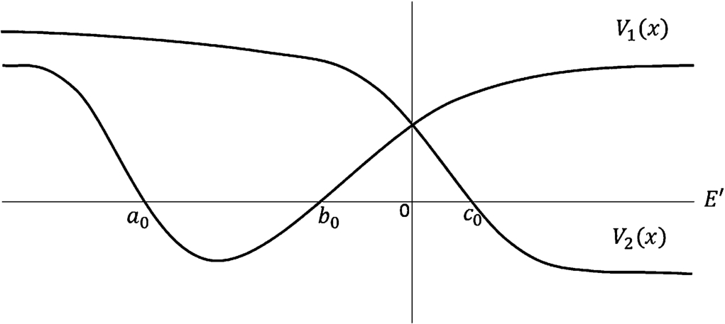
Here, as in [3] we study matrix system, the diagonal part of which consists of semiclassical Schrödinger operators, and the off-diagonal parts of first order differential operators. We assume that two potentials and cross transversally and that below the crossing admits a well, while is non-trapping (see Fig. 1). We study the resonances with imaginary parts and with real parts apart from the crossing and the bottom of the well by a constant distance independent of h. The real parts of the resonances behave like eigenvalues obtained from usual Bohr–Sommerfeld quantization condition for the well, that is, the leading terms of the real parts of the resonances satisfy , where a and b are the endpoints of the well. We also find that the widths of the resonances have exponential bounds as in [5,9] and under a condition on the interaction and the real part of the resonances they behave exactly like , where S is the Agmon distance for between endpoints b and c of the region where the potentials are greater than . In our model, the interaction is of the form and the condition on the interaction is that , where we assume the position of the crossing is . This result should be compared with [15, Theorem 2.6] for the case of one well. Paying attention to the shape of the graph of on the real axis our exponential bound is expected.
The graph of the two potentials on the real axis.
To prove our main theorem, we construct solutions to the system on four intervals, because if we formally construct solutions on two intervals as in [3] the series in the solutions do not converge. We need to construct four solutions on each of the middle two intervals since the solutions on the left and right intervals are represented as linear combinations of the four solutions. To control the behavior of the series in the solutions, we need four fundamental solutions on each of the middle intervals. We choose the fundamental solutions so that formal leading terms in the solutions will really determine the order of the solution with respect to h. We study the connection of the solutions and calculate the transition matrix at the crossing and change the basis of the solutions in order that some of the elements of the transition matrix will be zero. This makes the calculation of the quantization condition simple and we can find exponentially small terms with the expected index.
The content of this paper is as follows. In Section 2 we give the assumptions and state our main result. In Section 3 we give some preliminaries. In particular, we introduce solutions to the scalar Schrödinger equations. In Section 4 we construct fundamental solutions on four intervals and give estimates on them. In Section 5 we give the solutions to the system on the four intervals. In Section 6 we study the connection of the solutions and change the bases of the solutions to make transition matrix suitable for the calculation of the quantization condition. In Section 7 the quantization condition is given. Using the quantizaion condition in Section 8 we prove the main theorem.
Assumptions and results
As in [3], we consider a Schrödinger operator of the type,
where , , and is the formal adjoint of W.
We suppose the following conditions on , (see Fig. 1) and , .
and are real-valued analytic functions on and extend to holomorphic functions in the complex domain,
where is a constant and .
For , admits limits as in Γ and there exists a real number such that
There exist real numbers such that
and on ;
on ;
on ;
on ;
on ,
Moreover, one has
and are bounded analytic functions on Γ, and and are real when x is real.
As in [3] we can define the resonances of P as eigenvalues of the operator P acting on where is a complex distortion of that coincides with for . We denote by the set of the resonances of P.
For small enough, we set . We fix arbitrarily large, and we study the resonances of P lying in the set
For , has only two solutions and we denote the solution with the smaller real part and the larger one by and respectively. We also denote the unique solution of for by . For we define the action,
Then our result is the following.
Under Assumptions (
(A1)
)–(
(A4)
), forsmall enough, one has,where’s are complex numbers that satisfy,uniformly aswhere
For the first term on the right-hand side of (2.2) to be a semiclassical equivalent of the width of the resonance for sufficiently small h, one needs the additional ellipticity condition of W that satisfies , where ρ is a positive constant independent of h.
Some preliminaries
As in [3] let be a sufficiently large number and be a function such that for x large enough, for and
for some constant . In the sequel we will use the following notation:
for real b and c where . For complex b and c, we denote by the same notation appropriate curves in the complex plane connecting the end points. Then small enough, and some positive constant C, we have
where the integral is taken along .
We fix and . Then we can define a function which depends analytically on with small enough and sufficiently close to as follows:
Similarly, we can define,
which depends analytically on and with small enough.
In the same way as in [3, Appendix A.2] we have solutions to for . We denote by and the Airy functions.
Let. Then,
For sufficiently small, the equationadmits two solutionsonwith sufficiently smallsuch that as,uniformly with respect tosmall enough, and as,
For sufficiently small, there exist two constantsand the solutionsto the equationonwith sufficiently smallsuch that,uniformly with respect tosmall enough, and as,whereand.
Similarly, we have two solutions on with sufficiently small with the asymptotic behavior,
The Wronskians and are independent of the variable x and satisfies
To see the growth and decay from the points b and c, we define the solutions on , on , on and on as follows:
where , .
Fundamental solutions
In this section we introduce fundamental solutions used to construct solutions to the system.
Fundamental solutions on
We define fundamental solutions
of and
of by setting for ,
where is the Wronskian of and and so on. Then , and satisfy
and satisfies
For an interval I and sufficiently small , let be a family of functions satisfying for , . For we define as the set of continuous functions u on I equipped with the norm . In the following, we consider families of functions , and families of operators , .
Note that and on and respectively for sufficiently small h. In view of the construction of solutions to the system, we prove,
As h goes toone has,Moreover, there exist complex numbersdepending on v such that,and
(i) First, we shall prove (4.1) and (4.6). We set,
By an integration by parts we have,
Using the asymptotics of and on and fixing some constant sufficiently large we obtain,
If , then,
If , then,
If , then,
If , then,
Hence, observing for , we have
uniformly with respect to . Thus we obtain
Moreover, regardless of or , we have
Hence we obtain
which completes the proof of (4.1). Observing
we estimate and by the similar calculation as above and obtain (4.6).
(ii) We shall prove (4.2) and (4.7). We set,
By an integration by parts we have,
Using the asymptotics of and on and fixing some constant sufficiently large we obtain,
If , then,
If , then,
If , then,
If , then,
Hence, observing that , we have
uniformly with respect ot . Thus we have
When , there exist constants small enough and such that
On the other hand, if with small enough there exist a constant such that
Finally, when there exist constants such that
Here we used . To prove this estimate we write
The first term is estimated as follows;
and the second term is estimated as follows;
where we used that for in the inequalities. Hence, we obtain
which completes the proof of (4.2). Noting that there exists a constant such that and , we estimate and by the similar calculation as above and obtain (4.7).
(iii) We shall prove (4.3) and (4.8). We set,
By an integration by parts we have,
We obtain,
If , then,
If , then,
If , then,
Hence, we have as . Thus we have
When or with small enough, there exist a constant such that
When there exist constants such that
Hence, we obtain
which completes the proof of (4.3). The equation (4.8) is obvious from the definition of .
(iv) We shall prove (4.4) and (4.9). We set,
By an integration by parts we have,
We obtain,
If , then,
If , then,
If , then,
Hence, we have as . Thus we have
When , there exist constants small enough and such that
On the other hand, if with small enough, there exist a constant α such that
Finally, when there exist constants such that
Hence, we obtain
which completes the proof of (4.4). Noting that there exists a constant such that and , we obtain (4.9) by the similar calculation as above.
(v) Finally, we shall prove (4.5) and (4.10). We shall estimate the terms in (4.11) We obtain for any ,
Hence, we have as . Thus we have
We have for any ,
Noting that there exists a constant such that , we obtain (4.10) by the similar calculation as above. □
Fundamental solutions on
We define the fundamental solutions of on as,
for .
Then, one can prove exactly as for Lemma 4.1 that we have,
As h goes toone has,Moreover, there exist complex numbersdepending on v such that,and
Fundamental solutions on and
For any we set
and , . We also define the fundamental solutions and of on and as,
for and
for respectively. Then one has the following lemma.
As h goes toone has,Moreover, there exist complex numberssuch that,and
We set,
By an integration by parts we have,
and
For any we have
Hence we have and there exists such that,
which proves (4.12). By the similar calculation we obtain (4.14).
Next we estimate . For any small enough, there exists such that,
If or , then for any ,
If , then for any
If , then for any ,
If and then,
If and then,
Hence we have . Moreover, when we have
When we have
which completes the proof of (4.13). By the similar calculation we obtain (4.15).
Finally, we shall prove (4.16). By an integration by parts we have
Since we have . As for the integral we have
which proves the estimate for the first element of (4.16). The estimate for the derivative follows from the similar calculation. □
As h goes toone has,Moreover, there exist complex numberssuch that,and
Solutions to the system
In this section, we construct solutions to (2.1) on each interval. By Lemma 4.1, the operators , and are when acting on , and respectively. Therefore, we can define
These are solutions to (2.1) on and we have,
as .
In the same way, the operators , and are when acting on , and respectively. Therefore, we can define
These are solutions to (2.1) on and we have,
as .
The following lemmas are consequences of Lemma 4.1, 4.2 and the definitions of fundamental solutions. The estimates for the derivatives follow observing that if v is any of the functions , , , the order of is that of times .
There exist complex numbers,and,such that,
There exist complex numbers,and,such that,
We also define the solutions on and . By Lemma 4.3 the operator and are when acting on and respectively. Thus we can define,
on and
on .
For these solutions we have the following proposition corresponding to [3, Proposition 4.1].
The solutionsand,satisfy,
Connection of the solutions
In this section we investigate the connection of the basis and and that of (resp., ) and (resp., ). We define the transition matrix T as follows:
From now on, we set,
One hasMoreover, one has,
First, we consider . By Cramer’s formula we see that
For the calculation of Wronskians, we will use the following notation: If w is any of the vectors of functions , and written as
we set,
To estimate the remainder terms in w we notice
By Lemma 5.1, Lemma 5.2 and (6.6) we have
The Wronskian is written as the determinant
We calculate the determinant using the multilinearity with respect to columns. We regard each column in the determinant as the sum of vectors whose upper or lower two elements are 0, and expand the determinant into determinants whose columns are such vectors. Then the order of the upper and lower two elements in the remainder terms in (6.7) are those of the upper or lower two elements of the leading terms multiplied by . Thus by (3.1) and the definitions of and , we have
By (6.5), (6.8) and (6.9) we obtain (6.1). By the similar calculation we obtain (6.2).
Next we study and . For the calculation of higher order terms we notice
Since , we have
As for the derivative of , for x near 0 we have
We apply the stationary phase theorem to . Estimating the derivatives of near 0 by Cauchy’s integral formula, we have
Here we used . From (6.11), (6.12) and that
(6.3) follows. In the similar way we can obtain (6.4).
As for , since by Lemmas 5.1 and 5.2 upper two elements of , and can be written as
we have . As for , since we can see by Lemmas 5.1 and 5.2 that we need to choose remainder terms from at least two columns of the determinant , we obtain . The estimates for the other terms can be obtained by the similar way as above. □
To make some of the elements of the transition matrix 0, we change the basis on and .
There exist complex numbers,,,,such that if we set,the matrixdefined byhas the following form;withandhaving the same asymptotics asandrespectively. Moreover, we have the following estimates.
We define , , and by
Then, it is easy to see that has the form as in the lemma, and by Lemma 6.1 we have
□
Note that and have the same asymptotics as and with respect to h respectively. We next consider the connection of solutions at b and c.
Setas follows:whereandare WronskiansThen we have
We start with . By the Cramer’s formula we have
By Lemma 6.2 there exist such that
We use the notation w as in the proof of Lemma 6.1. The Wronskian in the right-hand side is written as the determinant;
By Lemma 4.3 we have
By Lemma 4.1 we also have
We calculate the determinant using the multilinearity with respect to columns as in the proof of Lemma 6.1. Then the order of the upper and lower two elements in the remainder terms in (6.26) and (6.27) are those of the leading terms multiplied by . Thus we obtain
From the definition we have , . Hence by Proposition 3.3 we obtain
Since and , we have
which completes the proof of (6.14). The proof of (6.15) is similar.
The estimates (6.16) and (6.17) follow from the calculation of the determinant as above, Lemma 4.1 and Lemma 4.3. We can prove (6.18) by the similar calculation as in the proof of (6.14). The estimate (6.19) is obtained using . The estimates (6.20)–(6.25) are obtained in the same way as (6.14)–(6.19). □
Quantisation condition
is a resonance of P if and only if,whereandare analytic for,is real for real E and
As in [3], E is a resonance if and only if , , and are linearly dependent, that is
We substitute the right-hand side of (6.13) for in (7.2) and develop the Wronskian as a sum of terms of the form where is a constant, and are chosen from , () and , () respectively. If only one of the , () is chosen from or , then by the form of in Lemma 6.2 we can see that . Thus by Lemma 6.3 we have
By Lemma 6.2 we can easily see that
and by Lemma 6.3 we have
where uniformly with respect to . From the construction of and we can easily see that is real for real E. We can also see by the similar calculation as in the proof of Lemma 6.1,
By (7.3), (7.4), (7.5) and asymptotics of and , we have
Therefore, is equivalent to
In order to solve (7.1), we first observe that the roots of are given by with,
For sufficiently small we set . Then since there exist constants such that for we have , the estimate holds. Since is holomorphic in (see, e.g., Fujiié-Ramond [4]), by the Cauchy’s integral formula we have for fixed and such that
Since for , and
by the Rouché’s theorem we can see that for sufficiently large and sufficiently small , has a unique solution in for and conversely, all the roots in are of this type. Since is real for and by (8.1) there exists a number such that , we can see that is real.
Estimating the remainder terms by the Cauchy’s integral formula as above, the left-hand side of (7.1) is written as
Thus again by the Rouché’s theorem we can see that for sufficiently large and sufficiently small , has a unique solution in
and all the roots in are of this type. In the same way as above we also have
Hence substituting into (7.1) for z we can see
from which Theorem 2.1 follows.
Footnotes
Acknowledgements
The author deeply thanks Professor A. Martinez for suggesting the topic treated in this paper and for his helpful discussions. This work was supported by JSPS KAKENHI Grant Number JP16J05967.
References
1.
H.Baklouti, Asymptotique des largeurs de résonances pour un modéle d’effet tunnel microlocal, Ann. Inst. H. Poincaré Phys. Theor.68 (1998), 179–228.
2.
J.M.Combes, P.Duclos, M.Klein and R.Seiler, The shape resonance, Commun. Math. Phys.110 (1987), 215–236. doi:10.1007/BF01207364.
3.
S.Fujiié, A.Martinez and T.Watanabe, Molecular predissociation resonances near an energy-level crossing I: Elliptic interaction, J. Differential Equations260 (2016), 4051–4085. doi:10.1016/j.jde.2015.11.015.
4.
S.Fujiié and T.Ramond, Matrice de scattering et résonances associées à une orbite hétérocline, Ann. Inst. H. Poincaré Phys. Theor.69 (1998), 31–82.
5.
A.Grigis and A.Martinez, Resonance widths for the molecular predissociation, Anal. PDE7 (2014), 1027–1055. doi:10.2140/apde.2014.7.1027.
6.
A.Grigis and A.Martinez, Resonance widths in a case of multidimensional phase space tunneling, Asymptotic Anal.391 (2015), 33–90.
7.
B.Helffer and J.Sjöstrand, Résonances en limite semi-classique, Mém. Soc. Math. France24–25 (1986), 1–228.
8.
P.D.Hislop and I.M.Sigal, Introduction to Spectral Theory: With Applications to Schrödinger Operators, Appl. Math. Sci., Vol. 113, Springer-Verlag, New York, 1996.
9.
M.Klein, On the mathematical theory of predissociation, Ann. Physics178 (1987), 48–73. doi:10.1016/S0003-4916(87)80012-X.
10.
M.Klein, A.Martinez, R.Seiler and X.P.Wang, On the Born–Oppenheimer expansions for polyatomic molecules, Commun. Math. Phys.143 (1992), 607–639. doi:10.1007/BF02099269.
11.
A.Martinez, Estimates on complex interactions in phase space, Math. Nachr.167 (1994), 203–254. doi:10.1002/mana.19941670109.
12.
A.Martinez and B.Messirdi, Resonances of diatomic molecules in the Born–Oppenheimer approximation, Comm. Partial Differential Equations19(7–8) (1994), 1139–1162. doi:10.1080/03605309408821048.
13.
A.Martinez and V.Sordoni, Twisted pseudodifferential calculus and application to the quantum evolution of molecules, Mem. AMS936 (2009), 1–82.
14.
S.Nakamura, On an example of phase-space tunneling, Ann. Inst. H. Poincaré Phys. Theor.63 (1995), 221–229.
15.
E.Servat, Résonances en dimension un pour l’opérateur de Schrödinger, Asymptotic Anal.39 (2004), 187–224.
16.
D.R.Yafaev, The semiclassical limit of eigenfunctions of the Schrödinger equation and the Bohr–Sommerfeld quantization condition, revisited, Algebra i Analiz22(6) (2010), 270–291. (Translation in St. Petersburg Math. J.22 (2011), 1051–1067.)