Topological asymptotic analysis of an optimal control problem modeled by a coupled system

Abstract

In this paper, we deal with the topological asymptotic analysis of an optimal control problem modeled by a coupled system. The control is a geometrical object and the cost is given by the misfit between a target function and the state, solution of the Helmholtz–Laplace coupled system. Higher-order topological derivatives are used to devise a non-iterative algorithm to compute the optimal control for the problem of interest. Numerical examples are presented in order to demonstrate the effectiveness of the proposed algorithm.

Keywords

Control problem Helmholtz–Laplace coupled system topological asymptotic analysis topological derivatives topology optimization

1. Introduction

Optimal control problems have a very long history and at the early stage it was seen as the advancement of the calculus of variations introduced by Euler. Classically, the control used to be considered in a subset of functional spaces, but later mathematicians started to consider more general control functions. See the references [6,18–21,30] for optimal control problems and derivation of optimality systems. We consider the control related to the topology of the subdomains of a domain in $R^{2}$ . To be more precise, we are dealing with an optimal control problem where the admissible set of controls contain the topological objects which do not have an algebraic structure which makes the problem more sophisticated.

Among the methods dealing with optimal control problems where the controls are geometrical objects, we want to draw the attention of the readers on the level-set methods [16,28,29,33] and the methods based on asymptotic expansions. In this paper, we are interested in a method of the second type based on the concept of the topological derivative. This concept was introduced by Sokołowski and Żochowski [34]. It has been successfully applied to many relevant scientific and engineering problems such as inverse problems [1,7,8,12,14,31], topology optimization [3,5,22,23], fracture mechanics [38,39], multi-scale constitutive modeling [4] and image processing [13]. According to Rocha and Novotny [31], the topological derivative leads to first-order iterative methods, but in contrast to the level-set methods, they are free of initial guess. In addition, the notion of second order topological derivative (see [11]) has been used to devise a class of second order non-iterative methods [7,8,13,24] which, in turn, are also free of initial guess. It motivates us to analyze this problem using higher-order topological derivatives. For more details related to asymptotic analysis of optimal control problems in the case where the control is a geometrical subdomain, we refer the reader to [17,35,40]. For the theoretical developments on the concepts of topological derivatives, one can see for instance [2,27,32].

In this paper, we study an optimal control problem of constructing an optimal geometrical object embedded in an open and bounded domain $Ω \subseteq R^{2}$ with smooth boundary $\partial Ω$ . We analyze the optimality of the cost evaluated in a subdomain $Ω_{o}$ of the domain Ω which is relatively compact in Ω. The state corresponding to a particular control in this optimization problem is considered to be the solution of a coupled Helmholtz–Laplace system posed in the domain Ω with Robin boundary condition on $\partial Ω$ . On the other hand, the control problem to be investigated can be seen as an inverse problem consisting in the reconstruction of a geometrical object from partial measurements of the solution to a coupled Helmholtz–Laplace system taken in $Ω_{o}$ . The associated inverse problem is motivated by the open problem proposed by Isakov [15, pp. 126, Problem 4.2]. See Remark 9 in Section 6.2.

The Helmholtz Equation appears in the study of acoustic waves. If the medium of propagation of sound wave is homogeneous, the wave number is a positive real number representing the property of the material. Similarly, if one studies the propagation of sound waves in an inhomogeneous medium, the wave number is a function away from zero. In the latter case, the mathematical analysis inherits the complication from the nature of the problem. One can see the book by Colton and Kress [10] for details. In this article, our objective is to study the topological asymptotic behavior of an optimal control problem. Therefore, for the sake of simplicity, we consider the wave number to be an indicator function, which gives rise to the fact that the state satisfies a coupled Helmholtz–Laplace system. This simplification, actually helps up to understand the deeper difficulties involved in the inverse problem whose forward equation is modeled by the inhomogeneous Helmholtz Equation with Cauchy data which will appear in our forthcoming projects.

The paper is organized as follows. The notion of topological derivatives is briefly recalled in Section 2. The optimal control problem is described in Section 3 where we also introduce some relevant cost functionals and auxiliary boundary value problems in order to use the theory of the topological derivatives to solve the problem of interest. The topological asymptotic expansion of the cost functional is presented in Section 4, which is the main result of this article. A complete proof of the main result is provided in Section 5, which includes the a priori estimates of the remainders obtained in Section 4. The computational part of this paper is presented in Section 6 where the non-iterative algorithm is devised and some numerical experiments showing the effectiveness of the proposed algorithm are presented.

2. Topological derivatives

The topological derivative is the first term of the asymptotic expansion of a given shape functional with respect to the small parameter which measures the size of singular domain perturbations, such as holes, inclusions, source-terms, cracks, etc. To be familiar with the concepts of topological derivatives, the reader may refer to the book by Novotny & Sokołowski [27]. However, for the sake of completeness of the manuscript, we briefly present below the main definitions and characteristics of the topological derivatives.

In general, an open and bounded domain $Ω \subset R^{d}$ , $d ⩾ 2$ , is perturbed by introducing nonsmooth features confined in a small region $ω_{ε} (ξ)$ of size $ε > 0$ centred at $ξ \in Ω$ such that $\overline{ω_{ε} (ξ)} \subset Ω$ . We define a characteristic function having support in the unperturbed domain Ω of the form $χ = 1_{Ω}$ . Similarly, we introduce a characteristic function $χ_{ε} (ξ)$ associated to the topologically perturbed domain. For example, in the case of holes as the perturbation $ω_{ε} (ξ)$ , we can write $χ_{ε} (ξ) = 1_{Ω} - 1_{\overline{ω_{ε} (ξ)}}$ and the singularly perturbed domain can be represented by $Ω_{ε} (ξ) = Ω ∖ \overline{ω_{ε} (ξ)}$ . Further, one assumes that a given shape functional $ψ (χ_{ε} (ξ))$ associated to the topologically perturbed domain $Ω_{ε} (ξ)$ admits the following topological asymptotic expansion $\begin{matrix} (2.1) & ψ (χ_{ε} (ξ)) = ψ (χ) + f (ε) D_{T} ψ (ξ) + o (f (ε)), \end{matrix}$ where $ψ (χ)$ is the shape functional associated to the reference (unperturbed) domain Ω and $f (ε)$ is a positive function depending upon the size ε of the topological perturbation such that $f (ε) \to 0$ when $ε ↓ 0$ . The function $ξ \mapsto D_{T} ψ (ξ)$ is called the first order topological derivative of the shape functional ψ at ξ. Mathematically, we can express it as $\begin{matrix} (2.2) & D_{T} ψ (ξ) : = lim_{ε \to 0} \frac{ψ (χ_{ε} (ξ)) - ψ (χ)}{f (ε)} . \end{matrix}$ Similarly, the second order topological derivative of the shape functional ψ at ξ can be obtained by expanding the remainder term $o (f (ε))$ in (2.1). More precisely, we will get the topological asymptotic expansion $\begin{matrix} (2.3) & ψ (χ_{ε} (ξ)) = ψ (χ) + f (ε) D_{T} ψ (ξ) + f_{2} (ε) D_{T}^{2} ψ (ξ) + o (f_{2} (ε)), \end{matrix}$ where $f_{2} (ε)$ is such that $\begin{matrix} (2.4) & lim_{ε \to 0} \frac{f_{2} (ε)}{f (ε)} = 0 . \end{matrix}$ Thus, the second order topological derivative can be defined as $\begin{matrix} (2.5) & D_{T}^{2} ψ (ξ) : = lim_{ε \to 0} \frac{ψ (χ_{ε} (ξ)) - ψ (χ) - f (ε) D_{T} ψ (ξ)}{f_{2} (ε)} . \end{matrix}$ Furthermore, one can define higher order topological derivatives by arguing analogically.

3. Problem formulation

The optimal control problem, whose state is a solution of the Helmholtz–Laplace coupled system, is formulated below. Some tools related to the theory of topological derivatives are introduced in order to compute the solution of the problem of interest.

In this article, for a given positive number $k > 0$ , positive integer $M \in Z^{+}$ and desired target $z^{m}$ , for $m = 1, \dots, M$ , we consider the optimal control problem $\begin{matrix} (3.1) & \underset{ω \subset A}{Minimize} J_{ω} (u^{1}, \dots, u^{M}) = \sum_{m = 1}^{M} \int_{Ω_{o}} (u^{m} - z^{m}) \overline{(u^{m} - z^{m})}, \end{matrix}$ where $A$ is an admissible set of all relatively compact ball shaped subdomains of the domain Ω. Moreover, $\overline{(u^{m} - z^{m})}$ represents the complex conjugate of $(u^{m} - z^{m})$ . Notice that the state $u^{m} = (u_{1}^{m}, u_{2}^{m})$ is the solution of the following coupled boundary value problem $\begin{matrix} (3.2) & \{\begin{matrix} Δ u_{1}^{m} + k^{2} u_{1}^{m} = 0 & in ω, \\ Δ u_{2}^{m} = 0 & in Ω ∖ \overline{ω}, \\ u_{1}^{m} = u_{2}^{m} & on \partial ω, \\ \partial_{ν} u_{1}^{m} = \partial_{ν} u_{2}^{m} & on \partial ω, \\ \partial_{n} u_{2}^{m} + i k u_{2}^{m} = g^{m} & on \partial Ω, \end{matrix} \end{matrix}$ for a given Robin data $g^{m} \in H^{- 1 / 2} (\partial Ω)$ with $m = 1, \dots, M$ . Here $i$ is the imaginary number, i.e., $i = \sqrt{- 1}$ . Moreover, ν and n are the outward unit normals to the boundaries $\partial ω$ and $\partial Ω$ , respectively. The reader interested in the mathematical aspects of such a boundary value problems may refer to the book by Nazarov and Plamenevsky [26], for instance. Concerning the numerical issues related to the coupled system (3.2), see [25]. Our objective is not to discuss the existence/uniqueness of the optimal control for the problem (3.1) using standard arguments. Instead, we are interested in constructing the optimal control using the concept of topological derivatives which, depending upon the desired target, ensures the existence of the optimal control. We also demonstrate the effectiveness of the method through few numerical results.

Fig. 1.

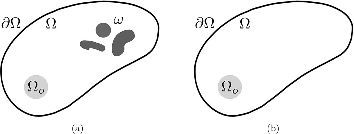
(a) Domain Ω with a set of perturbations ω and (b) Domain Ω without perturbations.

In principle, when we analyze an optimization problem using topological derivatives, we consider the unperturbed and the perturbed cost functionals to observe the rate of change of their behaviour with respect to the introduced perturbation. In particular, we introduce the unperturbed cost functional by taking $ω = \emptyset$ (see Fig. 1(b)) from $A$ as $\begin{matrix} (3.3) & J_{0} (u_{0}^{1}, \dots, u_{0}^{M}) = \sum_{m = 1}^{M} \int_{Ω_{o}} (u_{0}^{m} - z^{m}) \overline{(u_{0}^{m} - z^{m})} \end{matrix}$ where, for $m = 1, \dots, M$ , $u_{0}^{m}$ is the solution of the boundary value problem $\begin{matrix} (3.4) & \{\begin{matrix} Δ u_{0}^{m} = 0 & in Ω, \\ \partial_{n} u_{0}^{m} + i k u_{0}^{m} = g^{m} & on \partial Ω . \end{matrix} \end{matrix}$ Then, we introduce some perturbation $B_{ε} (ξ)$ into the domain Ω and consider the corresponding perturbed cost functional $\begin{matrix} (3.5) & J_{ε} (u_{ε}^{1}, \dots, u_{ε}^{M}) = \sum_{m = 1}^{M} \int_{Ω_{o}} (u_{ε}^{m} - z^{m}) \overline{(u_{ε}^{m} - z^{m})}, \end{matrix}$ where, $m = 1, \dots, M$ , $u_{ε}^{m} = (u_{ε, 1}^{m}, u_{ε, 2}^{m})$ is the solution to the following boundary value problem $\begin{matrix} (3.6) & \{\begin{matrix} Δ u_{ε, 1}^{m} + k^{2} u_{ε, 1}^{m} = 0 & in B_{ε} (ξ), \\ Δ u_{ε, 2}^{m} = 0 & in Ω ∖ \overline{B_{ε} (ξ)}, \\ u_{ε, 1}^{m} = u_{ε, 2}^{m} & on \partial B_{ε} (ξ), \\ \partial_{ν} u_{ε, 1}^{m} = \partial_{ν} u_{ε, 2}^{m} & on \partial B_{ε} (ξ), \\ \partial_{n} u_{ε, 2}^{m} + i k u_{ε, 2}^{m} = g^{m} & on \partial Ω . \end{matrix} \end{matrix}$

We are interested in approximating the optimal control in problem (3.1) by a set of circular subdomains of Ω, using the concept of topological derivatives. This approach provides us the explicit representation for the associated topological asymptotic expansion. Therefore, we consider an arbitrary number $N \in Z^{+}$ of circular balls of the form $\begin{matrix} (3.7) & B_{ε} (ξ) = B_{ε} (x_{1}, \dots, x_{N}) = ⋃_{i = 1}^{N} B_{ε_{i}} (x_{i}), \end{matrix}$ where $B_{ε_{i}} (x_{i})$ is a small circular perturbation with center $x_{i}$ and radius $ε_{i}$ , for $i = 1, \dots, N$ . Moreover, we assume that $\overline{B_{ε} (ξ)} \cap \partial Ω = \emptyset$ , $\overline{B_{ε} (ξ)} \cap Ω_{o} = \emptyset$ and $\overline{B_{ε_{i}} (x_{i})} \cap \overline{B_{ε_{j}} (x_{j})} = \emptyset$ for each $i \neq j$ and $i, j \in {1, \dots, N}$ .

Our main goal is to measure the sensitivity of the cost functional $J_{ω}$ defined in the optimal control problem (3.1) with respect to the parameters $(ε, ξ)$ related to the set of small perturbations $B_{ε} (ξ)$ using topological derivatives. In other words, our idea is to approximate the optimal control of the problem (3.1) by getting the number, size and location of the optimal perturbation. For this purpose, let us consider the difference between the perturbed cost functional $J_{ε} (u_{ε}^{1}, \dots, u_{ε}^{M})$ and its unperturbed counter-part $J_{0} (u_{0}^{1}, \dots, u_{0}^{M})$ defined in (3.5) and (3.3), respectively, which yields to the following simplified expression $\begin{matrix} (3.8) & J_{ε} (u_{ε}) - J_{0} (u_{0}) = \sum_{m = 1}^{M} \int_{Ω_{o}} [2 R {(u_{ε}^{m} - u_{0}^{m}) \overline{(u_{0}^{m} - z^{m})}} + (u_{ε}^{m} - u_{0}^{m}) \overline{(u_{ε}^{m} - u_{0}^{m})}], \end{matrix}$ where $u_{ε} = (u_{ε}^{1}, \dots, u_{ε}^{M})$ , $u_{0} = (u_{0}^{1}, \dots, u_{0}^{M})$ and $R {\cdot}$ denotes the real part of ${\cdot}$ .

Since the control ω is performed through a set of circular balls $B_{ε} (ξ)$ , we expand the perturbed functional $J_{ε} (u_{ε}^{1}, \dots, u_{ε}^{M})$ with respect to the Lebesgue measure (volume) of the two-dimensional ball $B_{ε_{i}} (x_{i})$ , namely, $| B_{ε_{i}} (x_{i}) | = π ε_{i}^{2}$ . To simplify the notation, we introduce the vector $\begin{matrix} (3.9) & α = (α_{1}, \dots, α_{N}) with α_{i} : = | B_{ε_{i}} (x_{i}) | . \end{matrix}$

Now we introduce some auxiliary boundary value problems whose solutions are functions which appear in the ansätz for the asymptotic expansion of $u_{ε}$ to be defined next. For each $i, j = 1, \dots, N$ and $m = 1, \dots, M$ , $h_{i}^{ε, m}$ is the solution of $\begin{matrix} (3.10) & \{\begin{matrix} Δ h_{i}^{ε, m} = - {(α_{i})}^{- 1} u_{0}^{m} χ_{B_{ε_{i}} (x_{i})} & in Ω, \\ \partial_{n} h_{i}^{ε, m} + i k h_{i}^{ε, m} = 0 & on \partial Ω, \end{matrix} \end{matrix}$ the function $h_{i j}^{ε, m}$ satisfies $\begin{matrix} (3.11) & \{\begin{matrix} Δ h_{i j}^{ε, m} = - {(α_{i})}^{- 1} h_{j}^{ε, m} χ_{B_{ε_{i}} (x_{i})} & in Ω, \\ \partial_{n} h_{i j}^{ε, m} + i k h_{i j}^{ε, m} = 0 & on \partial Ω, \end{matrix} \end{matrix}$ and ${\tilde{u}}_{ε}^{m} = ({\tilde{u}}_{ε, 1}^{m}, {\tilde{u}}_{ε, 2}^{m})$ is the solution to the following boundary value problem $\begin{matrix} (3.12) & \{\begin{matrix} Δ {\tilde{u}}_{ε, 1}^{m} + k^{2} {\tilde{u}}_{ε, 1}^{m} = - Φ_{ε}^{m} & in B_{ε} (ξ), \\ Δ {\tilde{u}}_{ε, 2}^{m} = 0 & in Ω ∖ \overline{B_{ε} (ξ)}, \\ {\tilde{u}}_{ε, 1}^{m} = {\tilde{u}}_{ε, 2}^{m} & on \partial B_{ε} (ξ), \\ \partial_{ν} {\tilde{u}}_{ε, 1}^{m} = \partial_{ν} {\tilde{u}}_{ε, 2}^{m} & on \partial B_{ε} (ξ), \\ \partial_{n} {\tilde{u}}_{ε, 2}^{m} + i k {\tilde{u}}_{ε, 2}^{m} = 0 & on \partial Ω, \end{matrix} \end{matrix}$ with $\begin{matrix} (3.13) & Φ_{ε}^{m} = k^{6} \sum_{i = 1}^{N} \sum_{j = 1}^{N} \sum_{l = 1}^{N} α_{j} α_{l} h_{j l}^{ε, m} χ_{B_{ε_{i}} (x_{i})} . \end{matrix}$

In order to simplify the analysis further, we write $h_{i}^{ε, m}$ as a sum of three functions $p_{i}^{ε}$ , $q_{i}$ and ${\tilde{h}}_{i}^{ε, m}$ in the form $\begin{matrix} (3.14) & h_{i}^{ε, m} = u_{0}^{m} (x_{i}) (p_{i}^{ε} + q_{i}) + {\tilde{h}}_{i}^{ε, m} . \end{matrix}$ The function $p_{i}^{ε}$ is a solution of $\begin{matrix} (3.15) & \{\begin{matrix} Δ p_{i}^{ε} = - {(α_{i})}^{- 1} χ_{B_{ε_{i}} (x_{i})} & in B_{R} (x_{i}), \\ p_{i}^{ε} = - {(2 π)}^{- 1} ln R & on \partial B_{R} (x_{i}), \end{matrix} \end{matrix}$ with $B_{ε_{i}} (x_{i}) \subset Ω \subset B_{R} (x_{i})$ , $x_{i} \in Ω$ , $ε ≪ R$ . By solving problem (3.15), one can observe that the solution $p_{i}^{ε}$ does not depend on ε outside the ball $B_{ε_{i}} (x_{i})$ . Therefore, we use the notation $p_{i} (x) : = p_{i}^{ε} (x)$ , $\forall x \in Ω ∖ \overline{B_{ε_{i}} (x_{i})}$ . Additionally, $q_{i}$ is the solution to the homogeneous boundary value problem $\begin{matrix} (3.16) & \{\begin{matrix} Δ q_{i} = 0 & in Ω, \\ \partial_{n} q_{i} + i k q_{i} = - \partial_{n} p_{i} - i k p_{i} & on \partial Ω, \end{matrix} \end{matrix}$ and ${\tilde{h}}_{i}^{ε, m}$ solves the boundary value problem $\begin{matrix} (3.17) & \{\begin{matrix} Δ {\tilde{h}}_{i}^{ε, m} = - {(α_{i})}^{- 1} (u_{0}^{m} - u_{0}^{m} (x_{i})) χ_{B_{ε_{i}} (x_{i})} & in Ω, \\ \partial_{n} {\tilde{h}}_{i}^{ε, m} + i k {\tilde{h}}_{i}^{ε, m} = 0 & on \partial Ω . \end{matrix} \end{matrix}$ From the decomposition (3.14) and the solution of the problem (3.15), we can introduce the notation $\begin{matrix} (3.18) & h_{i}^{ε, m} : = \{\begin{matrix} u_{0}^{m} (x_{i}) h_{i}^{ε} + {\tilde{h}}_{i}^{ε, m} & in B_{ε_{i}} (x_{i}), \\ u_{0}^{m} (x_{i}) h_{i} + {\tilde{h}}_{i}^{ε, m} & in Ω ∖ \overline{B_{ε_{i}} (x_{i})}, \end{matrix} \end{matrix}$ where $\begin{matrix} (3.19) & h_{i}^{ε} : = p_{i}^{ε} + q_{i} and h_{i} : = p_{i} + q_{i} . \end{matrix}$ Moreover, we also introduce an adjoint state $v^{m}$ as the solution of the following auxiliary boundary value problem $\begin{matrix} (3.20) & \{\begin{matrix} Δ v^{m} = (u_{0}^{m} - z^{m}) χ_{Ω_{o}} & in Ω, \\ \partial_{n} v^{m} - i k v^{m} = 0 & on \partial Ω . \end{matrix} \end{matrix}$

Finally, the ansätz for the asymptotic expansion of $u_{ε}$ can be defined in the following form $\begin{matrix} (3.21) & u_{ε}^{m} (x) = u_{0}^{m} (x) + k^{2} \sum_{i = 1}^{N} α_{i} h_{i}^{ε, m} (x) + k^{4} \sum_{i = 1}^{N} \sum_{j = 1}^{N} α_{i} α_{j} h_{i j}^{ε, m} (x) + {\tilde{u}}_{ε}^{m} (x), \end{matrix}$ with $h_{i}^{ε, m}$ , $h_{i j}^{ε, m}$ and ${\tilde{u}}_{m}^{ε}$ the solutions to the boundary value problems (3.10), (3.11) and (3.12), respectively.

4. Main theorem

In this section, we state our main result which consists in the closed form of the topological derivatives that appear in the topological asymptotic expansion of the perturbed cost functional. The asymptotic development of the cost functional in terms of the parameters related to N number of ball-shaped inclusions is completely described in Section 5.1.

In order to state the main result, we first introduce the vector $d \in R^{N}$ and the matrices $G, H \in R^{N \times N}$ whose entries are defined as $\begin{array}{l} (4.1) & d_{i} : = 2 k^{2} \sum_{m = 1}^{M} R {u_{0}^{m} (x_{i}) \overline{v^{m}} (x_{i})}, \\ (4.2) & G_{i i} : = \frac{k^{4}}{2 π} \sum_{m = 1}^{M} R {u_{0}^{m} (x_{i}) \overline{v^{m}} (x_{i})}, G_{i j} = 0, if i \neq j \end{array}$ and $\begin{array}{l} (4.3) & \begin{matrix} H_{i i} & : = - \frac{1 + log π^{2}}{2 π} k^{4} \sum_{m = 1}^{M} R {u_{0}^{m} (x_{i}) \overline{v^{m}} (x_{i})} - 4 k^{4} \sum_{m = 1}^{M} R {u_{0}^{m} (x_{i}) \overline{v^{m}} (x_{i}) q_{i} (x_{i})} \\ - \frac{k^{2}}{π} \sum_{m = 1}^{M} R {\nabla u_{0}^{m} (x_{i}) \cdot \nabla \overline{v^{m}} (x_{i})} + 2 k^{4} \sum_{m = 1}^{M} \int_{Ω_{o}} u_{0}^{m} (x_{i}) h_{i} \overline{u_{0}^{m}} (x_{i}) \overline{h_{i}}, \end{matrix} \\ (4.4) & H_{i j} : = - 4 k^{4} \sum_{m = 1}^{M} R {u_{0}^{m} (x_{j}) h_{j} (x_{i}) \overline{v^{m}} (x_{i})} + 2 k^{4} \sum_{m = 1}^{M} \int_{Ω_{o}} R {u_{0}^{m} (x_{i}) h_{i} \overline{u_{0}^{m}} (x_{j}) \overline{h_{j}}}, \end{array}$ if $i \neq j$ ; respectively, for $i, j = 1, \dots, N$ .

We are now in position to state the main result of this paper.

Theorem 1.
Let $q_{i}$ , $h_{i}$ for $i = 1, \dots, N$ and $u_{0}^{m}$ , $v^{m}$ for $m = 1, \dots, M$ be the functions defined in ( 3.16 ), ( 3.19 ) and ( 3.4 ), ( 3.20 ), respectively. Additionally, let d, G and H be the vector and the matrices whose entries are defined in ( 4.1 ), ( 4.2 ) and ( 4.3 )–( 4.4 ), respectively. Then, for the vector α introduced in ( 3.9 ), we have the following asymptotic expansion for the topologically perturbed cost functional $ψ (χ_{ε} (ξ)) : = J_{ε} (u_{ε})$ defined in ( 3.5 ): $\begin{matrix} (4.5) & ψ (χ_{ε} (ξ)) = ψ (χ) - α \cdot d (ξ) + G (ξ) α \cdot diag (α \otimes log α) + \frac{1}{2} H (ξ) α \cdot α + o (| α |^{2}), \end{matrix}$ where $ψ (χ) : = J_{0} (u_{0})$ is the topologically unperturbed cost functional from ( 3.3 ).

5. Proof of the main result

The proof of Theorem 1 is demonstrated in three steps. Firstly, we develop the asymptotic expansion of the topologically perturbed cost functional. Next, we prove a priori estimates related to the auxiliary states ${\tilde{h}}_{i}^{ε, m}$ , $h_{i}^{ε, m}$ , $h_{i j}^{ε, m}$ and ${\tilde{u}}_{ε}^{m}$ for $i, j = 1, \dots, N$ and $m = 1, \dots, M$ . Finally, in the last part of this section, the previously obtained results are used to estimate the remainders appeared in the first step. These estimates justify our topological asymptotic expansion (4.5).

5.1. Asymptotic development of the cost functional

Let us use (3.21) in (3.8), to obtain $\begin{matrix} (5.1) & \begin{matrix} J_{ε} (u_{ε}) - J_{0} (u_{0}) & = 2 k^{2} \sum_{m = 1}^{M} \sum_{i = 1}^{N} α_{i} \int_{Ω_{o}} R {h_{i}^{ε, m} \overline{(u_{0}^{m} - z^{m})}} \\ + 2 k^{4} \sum_{m = 1}^{M} \sum_{i = 1}^{N} \sum_{j = 1}^{N} α_{i} α_{j} \int_{Ω_{o}} R {h_{i j}^{ε, m} \overline{(u_{0}^{m} - z^{m})}} \\ + k^{4} \sum_{m = 1}^{M} \sum_{i = 1}^{N} \sum_{j = 1}^{N} α_{i} α_{j} \int_{Ω_{o}} h_{i}^{ε, m} \overline{h_{j}^{ε, m}} + \sum_{m = 1}^{M} \sum_{ℓ = 1}^{6} E_{ℓ}^{m} (ε), \end{matrix} \end{matrix}$ where $\begin{array}{l} (5.2) & E_{1}^{m} (ε) = 2 \int_{Ω_{o}} R {{\tilde{u}}_{ε}^{m} \overline{(u_{0}^{m} - z^{m})}}, \\ (5.3) & E_{2}^{m} (ε) = 2 k^{6} \sum_{i = 1}^{N} \sum_{j = 1}^{N} \sum_{l = 1}^{N} α_{i} α_{j} α_{l} \int_{Ω_{o}} R {h_{i}^{ε, m} \overline{h_{j l}^{ε, m}}}, \\ (5.4) & E_{3}^{m} (ε) = 2 k^{2} \sum_{i = 1}^{N} α_{i} \int_{Ω_{o}} R {h_{i}^{ε, m} \overline{{\tilde{u}}_{ε}^{m}}}, \\ (5.5) & E_{4}^{m} (ε) = k^{8} \sum_{i = 1}^{N} \sum_{j = 1}^{N} \sum_{l = 1}^{N} \sum_{p = 1}^{N} α_{i} α_{j} α_{l} α_{p} \int_{Ω_{o}} h_{i j}^{ε, m} \overline{h_{l p}^{ε, m}}, \\ (5.6) & E_{5}^{m} (ε) = 2 k^{4} \sum_{i = 1}^{N} \sum_{j = 1}^{N} α_{i} α_{j} \int_{Ω_{o}} R {h_{i j}^{ε, m} \overline{{\tilde{u}}_{ε}^{m}}} \end{array}$ and $\begin{matrix} (5.7) & E_{6}^{m} (ε) = \int_{Ω_{o}} {\tilde{u}}_{ε}^{m} \overline{{\tilde{u}}_{ε}^{m}} . \end{matrix}$

Now, let us introduce the weak formulation of the adjoint problem (3.20) to find $v^{m} \in H^{1} (Ω)$ such that $\begin{matrix} (5.8) & \int_{Ω} \nabla v^{m} \cdot \nabla \overline{η} - i k \int_{\partial Ω} v^{m} \overline{η} = - \int_{Ω_{o}} (u_{0}^{m} - z^{m}) \overline{η}, \forall η \in H^{1} (Ω) . \end{matrix}$ The weak formulations of (3.10) and (3.11) are to find $h_{i}^{ε, m} \in H^{1} (Ω)$ such that $\begin{matrix} (5.9) & \int_{Ω} \nabla h_{i}^{ε, m} \cdot \nabla \overline{η} + i k \int_{\partial Ω} h_{i}^{ε, m} \overline{η} = \frac{1}{α_{i}} \int_{B_{ε_{i}} (x_{i})} u_{0}^{m} \overline{η}, \forall η \in H^{1} (Ω) \end{matrix}$ and $h_{i j}^{ε, m} \in H^{1} (Ω)$ such that $\begin{matrix} (5.10) & \int_{Ω} \nabla h_{i j}^{ε, m} \cdot \nabla \overline{η} + i k \int_{\partial Ω} h_{i j}^{ε, m} \overline{η} = \frac{1}{α_{i}} \int_{B_{ε_{i}} (x_{i})} h_{j}^{ε, m} \overline{η}, \forall η \in H^{1} (Ω), \end{matrix}$ respectively.

By choosing $η = h_{i}^{ε, m}$ in (5.8) and $η = v^{m}$ in (5.9) as test functions and then considering the real part of the respective resulting equalities, we obtain $\begin{matrix} (5.11) & \int_{Ω_{o}} R {h_{i}^{ε, m} \overline{(u_{0}^{m} - z^{m})}} = - \frac{1}{α_{i}} \int_{B_{ε_{i}} (x_{i})} R {u_{0}^{m} \overline{v^{m}}} . \end{matrix}$ Similarly, if we choose $η = h_{i j}^{ε, m}$ in (5.8) and $η = v^{m}$ in (5.10) as test functions and then we consider the real part of the respective resulting equalities, it gives $\begin{matrix} (5.12) & \int_{Ω_{o}} R {h_{i j}^{ε, m} \overline{(u_{0}^{m} - z^{m})}} = - \frac{1}{α_{i}} \int_{B_{ε_{i}} (x_{i})} R {h_{j}^{ε, m} \overline{v^{m}}} . \end{matrix}$ By using (5.11) and (5.12) in (5.1), we get $\begin{matrix} (5.13) & \begin{matrix} J_{ε} (u_{ε}) - J_{0} (u_{0}) & = - 2 k^{2} \sum_{m = 1}^{M} \sum_{i = 1}^{N} \int_{B_{ε_{i}} (x_{i})} R {u_{0}^{m} \overline{v^{m}}} \\ - 2 k^{4} \sum_{m = 1}^{M} \sum_{i = 1}^{N} \sum_{j = 1}^{N} α_{j} \int_{B_{ε_{i}} (x_{i})} R {h_{j}^{ε, m} \overline{v^{m}}} \\ + k^{4} \sum_{m = 1}^{M} \sum_{i = 1}^{N} \sum_{j = 1}^{N} α_{i} α_{j} \int_{Ω_{o}} h_{i}^{ε, m} \overline{h_{j}^{ε, m}} + \sum_{m = 1}^{M} \sum_{ℓ = 1}^{6} E_{ℓ}^{m} (ε) . \end{matrix} \end{matrix}$ Taking into account the notations of (3.18), we get $\begin{matrix} (5.14) & \begin{matrix} J_{ε} (u_{ε}) - J_{0} (u_{0}) & = - 2 k^{2} \sum_{m = 1}^{M} \sum_{i = 1}^{N} \int_{B_{ε_{i}} (x_{i})} R {u_{0}^{m} \overline{v^{m}}} \\ - 2 k^{4} \sum_{m = 1}^{M} \sum_{i = 1}^{N} \sum_{\begin{array}{c} j = 1 \\ j \neq i \end{array}}^{N} α_{j} \int_{B_{ε_{i}} (x_{i})} R {u_{0}^{m} (x_{j}) h_{j} \overline{v^{m}}} \\ - 2 k^{4} \sum_{m = 1}^{M} \sum_{i = 1}^{N} α_{i} \int_{B_{ε_{i}} (x_{i})} R {u_{0}^{m} (x_{i}) h_{i}^{ε} \overline{v^{m}}} \\ + k^{4} \sum_{m = 1}^{M} \sum_{i = 1}^{N} \sum_{j = 1}^{N} α_{i} α_{j} \int_{Ω_{o}} u_{0}^{m} (x_{i}) h_{i} \overline{u_{0}^{m}} (x_{j}) \overline{h_{j}} + \sum_{m = 1}^{M} \sum_{ℓ = 1}^{10} E_{ℓ}^{m} (ε) . \end{matrix} \end{matrix}$ Here, for $m = 1, \dots, M$ , the new remainders are defined as $\begin{array}{l} (5.15) & E_{7}^{m} (ε) = - 2 k^{4} \sum_{i = 1}^{N} \sum_{\begin{array}{c} j = 1 \\ j \neq i \end{array}}^{N} α_{j} \int_{B_{ε_{i}} (x_{i})} R {{\tilde{h}}_{j}^{ε, m} \overline{v^{m}}}, \\ (5.16) & E_{8}^{m} (ε) = - 2 k^{4} \sum_{i = 1}^{N} α_{i} \int_{B_{ε_{i}} (x_{i})} R {{\tilde{h}}_{i}^{ε, m} \overline{v^{m}}}, \\ (5.17) & E_{9}^{m} (ε) = 2 k^{4} \sum_{i = 1}^{N} \sum_{j = 1}^{N} α_{i} α_{j} \int_{Ω_{o}} R {u_{0}^{m} (x_{i}) h_{i} \overline{{\tilde{h}}_{j}^{ε, m}}}, \\ (5.18) & E_{10}^{m} (ε) = k^{4} \sum_{i = 1}^{N} \sum_{j = 1}^{N} α_{i} α_{j} \int_{Ω_{o}} {\tilde{h}}_{i}^{ε, m} \overline{{\tilde{h}}_{j}^{ε, m}} . \end{array}$

The result (5.14) can be simplified further by noting that, in the first and the second terms of (5.14), we can consider the Taylor’s expansions of the functions $u_{0}^{m}$ , $v^{m}$ and $h_{j}$ around the point $x_{i}$ , with $\hat{x}$ being an intermediate point between x and $x_{i}$ . Let us denote the last nth term of the Taylor’s expansion of a function $f (x)$ around $x_{i}$ by $D^{n} f (\hat{x}) {(x - x_{i})}^{n}$ , $n ⩾ 1$ , $n \in N$ . In addition, in the third term of (5.14), we can use the explicit expression for the analytical part $p_{i}^{ε}$ of $h_{i}^{ε}$ in (3.19) inside the ball $B_{ε_{i}} (x_{i})$ .

Finally, after taking into account the above mentioned observations along with the decomposition (3.14) with the fact that $u_{0}^{m}$ and $v^{m}$ are harmonic outside $Ω_{o}$ , (5.14) takes the form $\begin{matrix} (5.19) & \begin{array}{l} J_{ε} (u_{ε}) - J_{0} (u_{0}) \\ = - 2 k^{2} \sum_{m = 1}^{M} \sum_{i = 1}^{N} α_{i} R {u_{0}^{m} (x_{i}) \overline{v^{m}} (x_{i})} + \frac{k^{4}}{2 π} \sum_{m = 1}^{M} \sum_{i = 1}^{N} α_{i}^{2} log α_{i} R {u_{0}^{m} (x_{i}) \overline{v^{m}} (x_{i})} \\ - \frac{1 + log π^{2}}{4 π} k^{4} \sum_{m = 1}^{M} \sum_{i = 1}^{N} α_{i}^{2} R {u_{0}^{m} (x_{i}) \overline{v^{m}} (x_{i})} - 2 k^{4} \sum_{m = 1}^{M} \sum_{i = 1}^{N} α_{i}^{2} R {u_{0}^{m} (x_{i}) \overline{v^{m}} (x_{i}) q_{i} (x_{i})} \\ - \frac{k^{2}}{2 π} \sum_{m = 1}^{M} \sum_{i = 1}^{N} α_{i}^{2} R {\nabla u_{0}^{m} (x_{i}) \cdot \nabla \overline{v^{m}} (x_{i})} - 2 k^{4} \sum_{m = 1}^{M} \sum_{i = 1}^{N} \sum_{\begin{array}{c} j = 1 \\ j \neq i \end{array}}^{N} α_{i} α_{j} R {u_{0}^{m} (x_{j}) h_{j} (x_{i}) \overline{v^{m}} (x_{i})} \\ + k^{4} \sum_{m = 1}^{M} \sum_{i = 1}^{N} \sum_{j = 1}^{N} α_{i} α_{j} \int_{Ω_{o}} u_{0}^{m} (x_{i}) h_{i} (x) \overline{u_{0}^{m}} (x_{j}) \overline{h_{j}} (x) + \sum_{m = 1}^{M} \sum_{ℓ = 1}^{20} E_{ℓ}^{m} (ε) . \end{array} \end{matrix}$ Now we have new remainders, namely, $\begin{array}{l} (5.20) & E_{11}^{m} (ε) = - 2 k^{2} \sum_{i = 1}^{N} \int_{B_{ε_{i}} (x_{i})} R {[\nabla u_{0}^{m} (x_{i}) \cdot (x - x_{i})] [D^{3} \overline{v^{m}} (\hat{x}) {(x - x_{i})}^{3}]}, \\ (5.21) & E_{12}^{m} (ε) = - 2 k^{2} \sum_{i = 1}^{N} \int_{B_{ε_{i}} (x_{i})} R {[D^{2} u_{0}^{m} (x_{i}) {(x - x_{i})}^{2}] [D^{2} \overline{v^{m}} (x_{i}) {(x - x_{i})}^{2}]}, \\ (5.22) & E_{13}^{m} (ε) = - 2 k^{2} \sum_{i = 1}^{N} \int_{B_{ε_{i}} (x_{i})} R {[\nabla \overline{v^{m}} (x_{i}) \cdot (x - x_{i})] [D^{3} u_{0}^{m} (\hat{x}) {(x - x_{i})}^{3}]}, \\ (5.23) & E_{14}^{m} (ε) = - 2 k^{2} \sum_{i = 1}^{N} \int_{B_{ε_{i}} (x_{i})} R {[D^{3} u_{0}^{m} (\hat{x}) {(x - x_{i})}^{3}] [D^{3} \overline{v^{m}} (\hat{x}) {(x - x_{i})}^{3}]}, \\ (5.24) & E_{15}^{m} (ε) = - 2 k^{4} \sum_{i = 1}^{N} \sum_{\begin{array}{c} j = 1 \\ j \neq i \end{array}}^{N} α_{j} \int_{B_{ε_{i}} (x_{i})} R {u_{0}^{m} (x_{j}) \overline{v^{m}} (x_{i}) D^{2} h_{j} (\hat{x}) {(x - x_{i})}^{2}}, \\ (5.25) & E_{16}^{m} (ε) = - 2 k^{4} \sum_{i = 1}^{N} \sum_{\begin{array}{c} j = 1 \\ j \neq i \end{array}}^{N} α_{j} \int_{B_{ε_{i}} (x_{i})} R {u_{0}^{m} (x_{j}) h_{j} (x_{i}) D^{2} \overline{v^{m}} (\hat{x}) {(x - x_{i})}^{2}}, \\ (5.26) & E_{17}^{m} (ε) = - 2 k^{4} \sum_{i = 1}^{N} \sum_{\begin{array}{c} j = 1 \\ j \neq i \end{array}}^{N} α_{j} \int_{B_{ε_{i}} (x_{i})} R {u_{0}^{m} (x_{j}) [\nabla \overline{v^{m}} (x_{i}) \cdot (x - x_{i})] [\nabla h_{j} (x_{i}) \cdot (x - x_{i})]}, \\ (5.27) & E_{18}^{m} (ε) = - 2 k^{4} \sum_{i = 1}^{N} \sum_{\begin{array}{c} j = 1 \\ j \neq i \end{array}}^{N} α_{j} \int_{B_{ε_{i}} (x_{i})} R {u_{0}^{m} (x_{j}) [D^{2} \overline{v^{m}} (\hat{x}) {(x - x_{i})}^{2}] [D^{2} h_{j} (\hat{x}) {(x - x_{i})}^{2}]}, \\ (5.28) & E_{19}^{m} (ε) = - 2 k^{4} \sum_{m = 1}^{M} \sum_{i = 1}^{N} α_{i} \int_{B_{ε_{i}} (x_{i})} R {u_{0}^{m} (x_{i}) (q_{i} \overline{v^{m}} - q_{i} (x_{i}) \overline{v^{m}} (x_{i}))}, \\ (5.29) & E_{20}^{m} (ε) = - 2 k^{4} \sum_{m = 1}^{M} \sum_{i = 1}^{N} α_{i} \int_{B_{ε_{i}} (x_{i})} R {u_{0}^{m} (x_{i}) p_{i}^{ε} (\overline{v^{m}} - \overline{v^{m}} (x_{i}))}, \end{array}$ for $m = 1, \dots, M$ .

Remark 2.
From the final expansion (5.19) we can obtain an estimate of the form $\begin{matrix} (5.30) & | J_{ε} (u_{ε}) - J_{0} (u_{0}) | ⩽ C k^{2} | ε |^{2}, \end{matrix}$ which corroborates with the result obtained in [37] in the context of singular domain perturbation. In addition, the topological derivatives in (5.19) are written in terms of point-wise values of the solutions $u_{0}^{m}$ , $v^{m}$ , $h_{j}$ , $q_{j}$ and the gradients of $u_{0}^{m}$ , $v^{m}$ . As suggested in [36], these values can be replaced by equivalent integrals over circles around the centers $x_{i}$ , $i = 1, \dots, N$ , allowing for overcoming regularity issues, if any.

5.2. Preliminary lemmas

In this section, we prove some estimates for the auxiliary states and residual terms which will be useful to get bounds for the remainders in the next section. We denote a positive constant independent of ε, i and m for $i = 1, \dots, N$ and $m = 1, \dots, M$ by C whose value changes according to the place it is used.

Lemma 3.
For $i = 1, \dots, N$ and $m = 1, \dots, M$ , let ${\tilde{h}}_{i}^{ε, m}$ be the weak solution of the problem ( 3.17 ). Then, there exists a C such that $\begin{matrix} (5.31) & {‖ {\tilde{h}}_{i}^{ε, m} ‖}_{H^{1} (Ω)} ⩽ C ε_{i}^{δ_{i}}, \forall i = 1, \dots, N and m = 1, \dots, M, \end{matrix}$ for any $0 < δ_{i} < 1$ .
Proof.
Let us choose ${\tilde{h}}_{i}^{ε, m}$ as a test function in the variational formulation of the problem (3.17) to get $\begin{matrix} (5.32) & \int_{Ω} \nabla {\tilde{h}}_{i}^{ε, m} \cdot \nabla \overline{{\tilde{h}}_{i}^{ε, m}} + i k \int_{\partial Ω} {\tilde{h}}_{i}^{ε, m} \overline{{\tilde{h}}_{i}^{ε, m}} = \frac{1}{α_{i}} \int_{B_{ε_{i}} (x_{i})} (u_{0}^{m} - u_{0}^{m} (x_{i})) \overline{{\tilde{h}}_{i}^{ε, m}} . \end{matrix}$ Using the Cauchy–Schwarz inequality and the interior elliptic regularity of the function $u_{0}^{m}$ , we get $\begin{array}{rcl} \int_{Ω} \nabla {\tilde{h}}_{i}^{ε, m} \cdot \nabla \overline{{\tilde{h}}_{i}^{ε, m}} + k \int_{\partial Ω} {\tilde{h}}_{i}^{ε, m} \overline{{\tilde{h}}_{i}^{ε, m}} & ⩽ & C ε_{i}^{- 2} {‖ u_{0}^{m} - u_{0}^{m} (x_{i}) ‖}_{L^{2} (B_{ε_{i}})} {‖ {\tilde{h}}_{i}^{ε, m} ‖}_{L^{2} (B_{ε_{i}})} \\ ⩽ & C ε_{i}^{- 2} ‖ x - x_{i} ‖_{L^{2} (B_{ε_{i}})} {‖ {\tilde{h}}_{i}^{ε, m} ‖}_{L^{2} (B_{ε_{i}})} \\ (5.33) & ⩽ & C {‖ {\tilde{h}}_{i}^{ε, m} ‖}_{L^{2} (B_{ε_{i}})}, \end{array}$ since $α_{i} \sim ε_{i}^{2}$ . Hölder inequality and the Sobolev embedding theorem provide us the inequality $\begin{matrix} (5.34) & {‖ {\tilde{h}}_{i}^{ε, m} ‖}_{L^{2} (B_{ε_{i}})} ⩽ C ε_{i}^{1 / q} {‖ {\tilde{h}}_{i}^{ε, m} ‖}_{L^{2 p} (B_{ε_{i}})} ⩽ C ε_{i}^{δ_{i}} {‖ {\tilde{h}}_{i}^{ε, m} ‖}_{H^{1} (Ω)}, \end{matrix}$ for any $1 < q < \infty$ with $1 / p + 1 / q = 1$ . If we denote $δ_{i} = 1 / q$ , we have $0 < δ_{i} < 1$ . Combining (5.33) and (5.34) with the coercivity of the Robin boundary value problem, we get the desired estimate (5.31). □
Corollary 4.
For any $0 < δ_{i}, δ_{j} < 1$ , there exists a C such that $\begin{matrix} (5.35) & {‖ {\tilde{h}}_{i}^{ε, m} ‖}_{L^{2} (B_{ε_{j}})} ⩽ C ε_{i}^{δ_{i}} ε_{j}^{δ_{j}}, \forall i, j = 1, \dots, N and m = 1, \dots, M, \end{matrix}$ where ${\tilde{h}}_{i}^{ε, m}$ is the weak solution of the problem ( 3.17 ).
Proof.
We can prove the desired result using Hölder inequality, Sobolev embedding theorem and Lemma 3. □
Lemma 5.
There exists a C such that $\begin{array}{l} (5.36) & {‖ h_{i}^{ε, m} ‖}_{L^{2} (B_{ε_{i}})} ⩽ C (ε_{i} | log ε_{i} | + ε_{i}^{2 δ_{i}}), \\ (5.37) & {‖ h_{i}^{ε, m} ‖}_{L^{2} (B_{ε_{j}})} ⩽ C (ε_{j} + ε_{i}^{δ_{i}} ε_{j}^{δ_{j}}), if i \neq j, \end{array}$ for any $0 < δ_{i}, δ_{j} < 1$ with $i, j = 1, \dots, N$ and $m = 1, \dots, M$ where $h_{i}^{ε, m}$ is defined in ( 3.14 ).
Proof.
Using the definition (3.14) with the triangular inequality, we get $\begin{matrix} (5.38) & {‖ h_{i}^{ε, m} ‖}_{L^{2} (B_{ε_{j}})} ⩽ C ({‖ p_{i}^{ε} ‖}_{L^{2} (B_{ε_{j}})} + ‖ q_{i} ‖_{L^{2} (B_{ε_{j}})} + {‖ {\tilde{h}}_{i}^{ε, m} ‖}_{L^{2} (B_{ε_{j}})}) . \end{matrix}$ Since the equation satisfied by $p_{i}^{ε}$ can be solved explicitly, we can establish the following estimates $\begin{matrix} (5.39) & {‖ p_{i}^{ε} ‖}_{L^{2} (B_{ε_{i}})} ⩽ C ε_{i} | log ε_{i} | \end{matrix}$ and $\begin{matrix} (5.40) & {‖ p_{i}^{ε} ‖}_{L^{2} (B_{ε_{j}})} ⩽ C ε_{j}, for i \neq j . \end{matrix}$ The interior elliptic regularity of function $q_{i}$ , Corollary 4 and the estimates (5.39)–(5.40) give us $\begin{array}{l} (5.41) & {‖ h_{i}^{ε, m} ‖}_{L^{2} (B_{ε_{i}})} ⩽ C (ε_{i} | log ε_{i} | + ε_{i} + ε_{i}^{2 δ_{i}}), \\ (5.42) & {‖ h_{i}^{ε, m} ‖}_{L^{2} (B_{ε_{j}})} ⩽ C (ε_{j} + ε_{i}^{δ_{i}} ε_{j}^{δ_{j}}), if i \neq j, \end{array}$ for any $0 < δ_{i}, δ_{j} < 1$ with $i, j = 1, \dots, N$ and $m = 1, \dots, M$ . Hence the fact. □
Lemma 6.
For $i = 1, \dots, N$ and $m = 1, \dots, M$ , let $h_{i}^{ε, m}$ be the weak solution of the problem ( 3.10 ). Then, there exists a C such that $\begin{matrix} (5.43) & {‖ h_{i}^{ε, m} ‖}_{H^{1} (Ω)} ⩽ C (\sqrt{| log ε_{i} |} + ε_{i}^{δ_{i} - 1 / 2}), \end{matrix}$ for any $0 < δ_{i} < 1$ .
Proof.
Let us take $h_{i}^{ε, m}$ as a test function in the weak formulation of (3.10) and use Cauchy–Schwarz inequality with the interior elliptic regularity of the function $u_{0}^{m}$ and Lemma 5 to get $\begin{array}{rcl} \int_{Ω} \nabla h_{i}^{ε, m} \cdot \nabla \overline{h_{i}^{ε, m}} + k \int_{\partial Ω} h_{i}^{ε, m} \overline{h_{i}^{ε, m}} & ⩽ & C ε_{i}^{- 2} {‖ u_{0}^{m} ‖}_{L^{2} (B_{ε_{i}})} {‖ h_{i}^{ε, m} ‖}_{L^{2} (B_{ε_{i}})} \\ ⩽ & C ε_{i}^{- 1} {‖ h_{i}^{ε, m} ‖}_{L^{2} (B_{ε_{i}})} \\ (5.44) & ⩽ & C (| log ε_{i} | + ε_{i}^{2 δ_{i} - 1}) . \end{array}$ Similar to the argument used in the proof of Lemma 3, we can use the coercivity of the Robin boundary value problem and (5.44) to have the desired result. □
Lemma 7.
For $i, j = 1, \dots, N$ and $m = 1, \dots, M$ , let $h_{i j}^{ε, m}$ be the weak solution of the problem ( 3.11 ). Then, there exists a C such that $\begin{array}{rcl} (5.45) & {‖ h_{i i}^{ε, m} ‖}_{H^{1} (Ω)} & ⩽ & C ε_{i}^{δ_{i} - 1} (| log ε_{i} | + ε_{i}^{2 δ_{i} - 1}), \\ (5.46) & {‖ h_{i j}^{ε, m} ‖}_{H^{1} (Ω)} & ⩽ & C ε_{i}^{δ_{i} - 1} (1 + ε_{i}^{δ_{i} - 1} ε_{j}^{δ_{j}}), if i \neq j, \end{array}$ for any $0 < δ_{i}, δ_{j} < 1$ .
Proof.
Let us take $h_{i j}^{ε, m}$ as a test function in the weak formulation of (3.11) and use the Cauchy–Schwarz inequality with Lemma 5 to have $\begin{array}{rcl} (5.47) & \int_{Ω} \nabla h_{i i}^{ε, m} \cdot \nabla \overline{h_{i i}^{ε, m}} + k \int_{\partial Ω} h_{i i}^{ε, m} \overline{h_{i i}^{ε, m}} & ⩽ & C ε_{i}^{- 1} (| log ε_{i} | + ε_{i}^{2 δ_{i} - 1}) {‖ h_{i i}^{ε, m} ‖}_{L^{2} (B_{ε_{i}})}, \\ (5.48) & \int_{Ω} \nabla h_{i j}^{ε, m} \cdot \nabla \overline{h_{i j}^{ε, m}} + k \int_{\partial Ω} h_{i j}^{ε, m} \overline{h_{i j}^{ε, m}} & ⩽ & C ε_{i}^{- 1} (1 + ε_{i}^{δ_{i} - 1} ε_{j}^{δ_{j}}) {‖ h_{i j}^{ε, m} ‖}_{L^{2} (B_{ε_{i}})}, \end{array}$ if $i \neq j$ . Hölder inequality and the Sobolev embedding theorem can be used to derive $\begin{matrix} (5.49) & {‖ h_{i j}^{ε, m} ‖}_{L^{2} (B_{ε_{i}})} ⩽ C ε_{i}^{1 / q} {‖ h_{i j}^{ε, m} ‖}_{L^{2 p} (B_{ε_{i}})} ⩽ C ε_{i}^{δ_{i}} {‖ h_{i j}^{ε, m} ‖}_{H^{1} (Ω)}, \end{matrix}$ for any $1 < q < \infty$ with $1 / p + 1 / q = 1$ . Like earlier, we denote $δ_{i} = 1 / q$ which implies $0 < δ_{i} < 1$ . Combining (5.47) and (5.49) with the coercivity of the Robin boundary value problem, we obtain the desired estimate (5.45). Analogously, we can obtain the estimate (5.46) from (5.48). □
Lemma 8.
For $m = 1, \dots, M$ , let ${\tilde{u}}_{ε}^{m}$ be the weak solution of the problem ( 3.12 ). Then, there exists a C such that $\begin{matrix} (5.50) & {‖ {\tilde{u}}_{ε}^{m} ‖}_{L^{2} (Ω_{o})} ⩽ C (1 + C k^{2} \overline{ε}) \sum_{i, j, l = 1}^{N} ε_{l}^{2 δ_{l}} ε_{i}^{δ_{i} + 1} (ε_{i}^{2} | log ε_{i} | + ε_{i}^{2 δ_{i} + 1} + ε_{j}^{2} + ε_{i}^{δ_{i} - 1} ε_{j}^{δ_{j} + 2}) \end{matrix}$ for any $0 < δ_{i}, δ_{j}, δ_{l} < 1$ with $\overline{ε} = max {ε_{i}^{2 δ_{i}}}$ , for $i, j, l = 1, \dots, N$ .
Proof.
Let us choose ${\tilde{u}}_{ε}^{m}$ as a test function in the weak formulation of (3.12) for $m = 1, \dots, M$ to get $\begin{matrix} (5.51) & \int_{Ω} \nabla {\tilde{u}}_{ε}^{m} \cdot \nabla \overline{{\tilde{u}}_{ε}^{m}} - k^{2} \sum_{l = 1}^{N} \int_{B_{ε_{l}} (x_{l})} {\tilde{u}}_{ε}^{m} \overline{{\tilde{u}}_{ε}^{m}} + i k \int_{\partial Ω} {\tilde{u}}_{ε}^{m} \overline{{\tilde{u}}_{ε}^{m}} = \int_{Ω} Φ_{ε}^{m} \overline{{\tilde{u}}_{ε}^{m}} . \end{matrix}$ Considering the real and imaginary part, we have $\begin{matrix} (5.52) & \int_{Ω} \nabla {\tilde{u}}_{ε}^{m} \cdot \nabla \overline{{\tilde{u}}_{ε}^{m}} - k^{2} \sum_{l = 1}^{N} \int_{B_{ε_{l}} (x_{l})} {\tilde{u}}_{ε}^{m} \overline{{\tilde{u}}_{ε}^{m}} = R {\int_{Ω} Φ_{ε}^{m} \overline{{\tilde{u}}_{ε}^{m}}} \end{matrix}$ and $\begin{matrix} (5.53) & k \int_{\partial Ω} {\tilde{u}}_{ε}^{m} \overline{{\tilde{u}}_{ε}^{m}} = Im {\int_{Ω} Φ_{ε}^{m} \overline{{\tilde{u}}_{ε}^{m}}}, \end{matrix}$ where $Im {\cdot}$ denotes the imaginary part of ${\cdot}$ . By summing (5.52) and (5.53), we get $\begin{matrix} (5.54) & \int_{Ω} \nabla {\tilde{u}}_{ε}^{m} \cdot \nabla \overline{{\tilde{u}}_{ε}^{m}} + k \int_{\partial Ω} {\tilde{u}}_{ε}^{m} \overline{{\tilde{u}}_{ε}^{m}} = R {\int_{Ω} Φ_{ε}^{m} \overline{{\tilde{u}}_{ε}^{m}}} + Im {\int_{Ω} Φ_{ε}^{m} \overline{{\tilde{u}}_{ε}^{m}}} + k^{2} \sum_{l = 1}^{N} \int_{B_{ε_{l}} (x_{l})} {\tilde{u}}_{ε}^{m} \overline{{\tilde{u}}_{ε}^{m}}, \end{matrix}$ from which the following inequality holds $\begin{matrix} (5.55) & \int_{Ω} \nabla {\tilde{u}}_{ε}^{m} \cdot \nabla \overline{{\tilde{u}}_{ε}^{m}} + k \int_{\partial Ω} {\tilde{u}}_{ε}^{m} \overline{{\tilde{u}}_{ε}^{m}} ⩽ C | \int_{Ω} Φ_{ε}^{m} \overline{{\tilde{u}}_{ε}^{m}} | + k^{2} \sum_{l = 1}^{N} \int_{B_{ε_{l}} (x_{l})} {\tilde{u}}_{ε}^{m} \overline{{\tilde{u}}_{ε}^{m}} . \end{matrix}$ Using the Cauchy–Schwarz inequality taking into account the definition of the function $Φ_{ε}^{m}$ given by (3.13), we obtain $\begin{matrix} (5.56) & \int_{Ω} \nabla {\tilde{u}}_{ε}^{m} \cdot \nabla \overline{{\tilde{u}}_{ε}^{m}} + k \int_{\partial Ω} {\tilde{u}}_{ε}^{m} \overline{{\tilde{u}}_{ε}^{m}} ⩽ C [\sum_{i, j, l = 1}^{N} ε_{i}^{2} ε_{j}^{2} {‖ h_{i j}^{ε, m} ‖}_{L^{2} (B_{ε_{l}})} {‖ {\tilde{u}}_{ε}^{m} ‖}_{L^{2} (B_{ε_{l}})} + k^{2} \sum_{l = 1}^{N} {‖ {\tilde{u}}_{ε}^{m} ‖}_{L^{2} (B_{ε_{l}})}^{2}] . \end{matrix}$ Hölder inequality and the Sobolev embedding theorem can be used to derive $\begin{matrix} (5.57) & {‖ {\tilde{u}}_{ε}^{m} ‖}_{L^{2} (B_{ε_{l}})} ⩽ C ε_{l}^{1 / q} {‖ {\tilde{u}}_{ε}^{m} ‖}_{L^{2 p} (B_{ε_{l}})} ⩽ C ε_{l}^{δ_{l}} {‖ {\tilde{u}}_{ε}^{m} ‖}_{H^{1} (Ω)}, \forall l = 1, \dots, N, \end{matrix}$ for any $1 < q < \infty$ with $1 / p + 1 / q = 1$ , where $δ_{l} = 1 / q$ which implies $0 < δ_{l} < 1$ . Combining (5.56) and (5.57), we have $\begin{matrix} (5.58) & \begin{array}{l} \int_{Ω} \nabla {\tilde{u}}_{ε}^{m} \cdot \nabla \overline{{\tilde{u}}_{ε}^{m}} + k \int_{\partial Ω} {\tilde{u}}_{ε}^{m} \overline{{\tilde{u}}_{ε}^{m}} \\ ⩽ C [\sum_{i, j, l = 1}^{N} ε_{l}^{δ_{l}} ε_{i}^{2} ε_{j}^{2} {‖ h_{i j}^{ε, m} ‖}_{L^{2} (B_{ε_{l}})} {‖ {\tilde{u}}_{ε}^{m} ‖}_{H^{1} (Ω)} + k^{2} \sum_{l = 1}^{N} ε_{l}^{2 δ_{l}} {‖ {\tilde{u}}_{ε}^{m} ‖}_{H^{1} (Ω)}^{2}] . \end{array} \end{matrix}$ Defining $\overline{ε} : = max {ε_{l}^{2 δ_{l}}}$ , for $l = 1, \dots, N$ , the last inequality can be rewritten as $\begin{matrix} (5.59) & \int_{Ω} \nabla {\tilde{u}}_{ε}^{m} \cdot \nabla \overline{{\tilde{u}}_{ε}^{m}} + k \int_{\partial Ω} {\tilde{u}}_{ε}^{m} \overline{{\tilde{u}}_{ε}^{m}} ⩽ C [\sum_{i, j, l = 1}^{N} ε_{l}^{δ_{l}} ε_{i}^{2} ε_{j}^{2} {‖ h_{i j}^{ε, m} ‖}_{L^{2} (B_{ε_{l}})} {‖ {\tilde{u}}_{ε}^{m} ‖}_{H^{1} (Ω)} + k^{2} \overline{ε} {‖ {\tilde{u}}_{ε}^{m} ‖}_{H^{1} (Ω)}^{2}] . \end{matrix}$ The coercivity of the Robin boundary value problem combined with the inequality above gives us $\begin{matrix} (5.60) & {‖ {\tilde{u}}_{ε}^{m} ‖}_{H^{1} (Ω)} ⩽ C (\frac{1}{1 - C k^{2} \overline{ε}}) \sum_{i, j, l = 1}^{N} ε_{l}^{δ_{l}} ε_{i}^{2} ε_{j}^{2} {‖ h_{i j}^{ε, m} ‖}_{L^{2} (B_{ε_{l}})} . \end{matrix}$ Taking into account that $\begin{matrix} (5.61) & \frac{1}{1 - C k^{2} \overline{ε}} = 1 + C k^{2} \overline{ε} + O ({\overline{ε}}^{2}), \end{matrix}$ we obtain, from (5.60), that $\begin{matrix} (5.62) & {‖ {\tilde{u}}_{ε}^{m} ‖}_{H^{1} (Ω)} ⩽ C (1 + C k^{2} \overline{ε}) \sum_{i, j, l = 1}^{N} ε_{l}^{δ_{l}} ε_{i}^{2} ε_{j}^{2} {‖ h_{i j}^{ε, m} ‖}_{L^{2} (B_{ε_{l}})} . \end{matrix}$ Analogously to the estimate obtained in (5.57), we use Hölder inequality and the Sobolev embedding theorem to derive $\begin{matrix} (5.63) & {‖ h_{i j}^{ε, m} ‖}_{L^{2} (B_{ε_{l}})} ⩽ C ε_{l}^{1 / q} {‖ h_{i j}^{ε, m} ‖}_{L^{2 p} (B_{ε_{l}})} ⩽ C ε_{l}^{δ_{l}} {‖ h_{i j}^{ε, m} ‖}_{H^{1} (Ω)}, \forall l = 1, \dots, N, \end{matrix}$ for any $1 < q < \infty$ with $1 / p + 1 / q = 1$ , where $δ_{l} = 1 / q$ which implies $0 < δ_{l} < 1$ . Combining (5.60) and (5.61) with Lemma 7, we get $\begin{matrix} (5.64) & {‖ {\tilde{u}}_{ε}^{m} ‖}_{H^{1} (Ω)} ⩽ C (1 + C k^{2} \overline{ε}) \sum_{i, j, l = 1}^{N} ε_{l}^{2 δ_{l}} ε_{i}^{δ_{i} + 1} (ε_{i}^{2} | log ε_{i} | + ε_{i}^{2 δ_{i} + 1} + ε_{j}^{2} + ε_{i}^{δ_{i} - 1} ε_{j}^{δ_{j} + 2}) . \end{matrix}$ The desired estimate is obtained from (5.64), taking into account that $‖ {\tilde{u}}_{ε}^{m} ‖_{L^{2} (Ω_{o})} ⩽ ‖ {\tilde{u}}_{ε}^{m} ‖_{H^{1} (Ω)}$ . □

5.3. A priori estimates of the remainders

We will successively prove that $| E_{ℓ}^{m} (ε) | = o (| ε |^{4})$ for $ℓ = 1, \dots, 20$ , where $| ε | : = ε_{1} + \dots + ε_{N}$ . For simplicity, we use the symbol C to denote any constant independent of ε.

5.3.1. Estimates for the remainders $E_{ℓ}^{m} (ε)$ , $ℓ = 1, \dots, 10$

We start by using the Cauchy–Schwarz inequality and then we use the appropriate lemmas of Section 5.2. Proceeding in this way, we obtain $\begin{array}{rcl} (5.65) & | E_{1}^{m} (ε) | ⩽ C {‖ {\tilde{u}}_{ε}^{m} ‖}_{L^{2} (Ω_{o})} {‖ u_{0}^{m} - z^{m} ‖}_{L^{2} (Ω_{o})} = o (| ε |^{4}), \end{array}$ for any $1 / 2 < δ < 1$ , where we have used Lemma 8; $\begin{array}{rcl} (5.66) & | E_{2}^{m} (ε) | ⩽ C | ε |^{6} \sum_{i = 1}^{N} {‖ h_{i}^{ε, m} ‖}_{H^{1} (Ω)} \sum_{j = 1}^{N} \sum_{l = 1}^{N} {‖ h_{j l}^{ε, m} ‖}_{H^{1} (Ω)} = o (| ε |^{4}), \end{array}$ for any $1 / 8 < δ < 1$ , where we have used Lemmas 6 and 7; $\begin{array}{rcl} (5.67) & | E_{3}^{m} (ε) | ⩽ C | ε |^{2} {‖ {\tilde{u}}_{ε}^{m} ‖}_{L^{2} (Ω_{o})} \sum_{i = 1}^{N} {‖ h_{i}^{ε, m} ‖}_{H^{1} (Ω)} = o (| ε |^{4}), \end{array}$ for any $1 / 10 < δ < 1$ , where we have used Lemmas 6 and 8; $\begin{array}{rcl} (5.68) & | E_{4}^{m} (ε) | ⩽ C | ε |^{8} \sum_{i = 1}^{N} \sum_{j = 1}^{N} {‖ h_{i j}^{ε, m} ‖}_{H^{1} (Ω)} \sum_{l = 1}^{N} \sum_{p = 1}^{N} {‖ h_{l p}^{ε, m} ‖}_{H^{1} (Ω)} = o (| ε |^{4}), \end{array}$ for any $0 < δ < 1$ , where we have used Lemma 7; $\begin{array}{rcl} (5.69) & | E_{5}^{m} (ε) | ⩽ C | ε |^{4} {‖ {\tilde{u}}_{ε}^{m} ‖}_{L^{2} (Ω_{o})} \sum_{i = 1}^{N} \sum_{j = 1}^{N} {‖ h_{i j}^{ε, m} ‖}_{H^{1} (Ω)} = o (| ε |^{4}), \end{array}$ for any $0 < δ < 1$ , where we have used Lemmas 7 and 8; $\begin{matrix} (5.70) & | E_{6}^{m} (ε) | ⩽ C {‖ {\tilde{u}}_{ε}^{m} ‖}_{L^{2} (Ω_{o})} {‖ {\tilde{u}}_{ε}^{m} ‖}_{L^{2} (Ω_{o})} = o (| ε |^{4}), \end{matrix}$ for any $0 < δ < 1$ , where we have used Lemma 8; $\begin{matrix} (5.71) & | E_{7}^{m} (ε) | ⩽ C | ε |^{3} \sum_{i = 1}^{N} \sum_{\begin{array}{c} j = 1 \\ j \neq i \end{array}}^{N} {‖ {\tilde{h}}_{j}^{ε, m} ‖}_{L^{2} (B_{ε_{i}})} = o (| ε |^{4}), \end{matrix}$ for any $1 / 2 < δ < 1$ , where we have used Corollary 4 together with the interior elliptic regularity of the function $v^{m}$ ; $\begin{matrix} (5.72) & | E_{8}^{m} (ε) | ⩽ C | ε |^{3} \sum_{i = 1}^{N} {‖ {\tilde{h}}_{i}^{ε, m} ‖}_{L^{2} (B_{ε_{i}})} = o (| ε |^{4}), \end{matrix}$ for any $1 / 2 < δ < 1$ , where we have use the same arguments as before; $\begin{array}{rcl} (5.73) & | E_{9}^{m} (ε) | ⩽ C | ε |^{4} \sum_{j = 1}^{N} {‖ {\tilde{h}}_{j}^{ε, m} ‖}_{H^{1} (Ω)} = o (| ε |^{4}), \end{array}$ for any $0 < δ < 1$ , where we have used Lemma 3; $\begin{array}{rcl} (5.74) & | E_{10}^{m} (ε) | ⩽ C | ε |^{4} \sum_{i = 1}^{N} {‖ {\tilde{h}}_{i}^{ε, m} ‖}_{H^{1} (Ω)} \sum_{j = 1}^{N} {‖ {\tilde{h}}_{j}^{ε, m} ‖}_{H^{1} (Ω)} = o (| ε |^{4}), \end{array}$ for any $0 < δ < 1$ , where we have used Lemma 3.

5.3.2. Estimates for the remainders $E_{ℓ}^{m} (ε)$ , $ℓ = 11, \dots, 19$

For the remainders of this section, the estimates are obtained as follows: we firstly use the Cauchy–Schwarz inequality and then we consider the fact that $‖ x - x_{i} ‖_{L^{2} (B_{ε_{i}})}^{n} = O (| ε |^{n + 1})$ , where $n \in Z^{+}$ . The estimates are $\begin{array}{rcl} (5.75) & | E_{11}^{m} (ε) | & ⩽ & C \sum_{i = 1}^{N} ‖ x - x_{i} ‖_{L^{2} (B_{ε_{i}})} ‖ x - x_{i} ‖_{L^{2} (B_{ε_{i}})}^{3} = O (| ε |^{6}); \\ (5.76) & | E_{12}^{m} (ε) | & ⩽ & C \sum_{i = 1}^{N} ‖ x - x_{i} ‖_{L^{2} (B_{ε_{i}})}^{2} ‖ x - x_{i} ‖_{L^{2} (B_{ε_{i}})}^{2} = O (| ε |^{6}); \\ (5.77) & | E_{13}^{m} (ε) | & ⩽ & C \sum_{i = 1}^{N} ‖ x - x_{i} ‖_{L^{2} (B_{ε_{i}})} ‖ x - x_{i} ‖_{L^{2} (B_{ε_{i}})}^{3} = O (| ε |^{6}); \\ (5.78) & | E_{14}^{m} (ε) | & ⩽ & C \sum_{i = 1}^{N} ‖ x - x_{i} ‖_{L^{2} (B_{ε_{i}})}^{3} ‖ x - x_{i} ‖_{L^{2} (B_{ε_{i}})}^{3} = O (| ε |^{8}); \\ (5.79) & | E_{15}^{m} (ε) | & ⩽ & C | ε |^{2} \sum_{i = 1}^{N} ‖ x - x_{i} ‖_{L^{2} (B_{ε_{i}})}^{2} ‖ 1 ‖_{L^{2} (B_{ε_{i}})} = O (| ε |^{6}); \\ (5.80) & | E_{16}^{m} (ε) | & ⩽ & C | ε |^{2} \sum_{i = 1}^{N} ‖ x - x_{i} ‖_{L^{2} (B_{ε_{i}})}^{2} ‖ 1 ‖_{L^{2} (B_{ε_{i}})} = O (| ε |^{6}); \\ (5.81) & | E_{17}^{m} (ε) | & ⩽ & C | ε |^{2} \sum_{i = 1}^{N} ‖ x - x_{i} ‖_{L^{2} (B_{ε_{i}})} ‖ x - x_{i} ‖_{L^{2} (B_{ε_{i}})} = O (| ε |^{6}); \\ (5.82) & | E_{18}^{m} (ε) | & ⩽ & C | ε |^{2} \sum_{i = 1}^{N} ‖ x - x_{i} ‖_{L^{2} (B_{ε_{i}})}^{2} ‖ x - x_{i} ‖_{L^{2} (B_{ε_{i}})}^{2} = O (| ε |^{8}); \end{array}$ and $\begin{array}{rcl} | E_{19}^{m} (ε) | & ⩽ & C | ε |^{2} \sum_{i = 1}^{N} {‖ q_{i} v^{m} - q_{i} (x_{i}) v^{m} (x_{i}) ‖}_{L^{2} (B_{ε_{i}})} ‖ 1 ‖_{L^{2} (B_{ε_{i}})} \\ (5.83) & ⩽ & C | ε |^{3} \sum_{i = 1}^{N} ‖ x - x_{i} ‖_{L^{2} (B_{ε_{i}})} = O (| ε |^{5}), \end{array}$ where we have used the interior elliptic regularity of the functions $q_{i}$ and $v^{m}$ .

5.3.3. Estimate for the remainder $E_{20}^{m} (ε)$

Here, the Cauchy–Schwarz inequality and the explicit expression of $p_{i}^{ε}$ in the ball $B_{ε_{i}} (x_{i})$ , for $i = 1, \dots, N$ , are used to obtain the estimate of the last remainder. Proceeding in this way, we get $\begin{array}{rcl} | E_{20}^{m} (ε) | & ⩽ & C | ε |^{2} \sum_{i = 1}^{N} {‖ p_{i}^{ε} ‖}_{L^{2} (B_{ε_{i}})} {‖ v^{m} - v^{m} (x_{i}) ‖}_{L^{2} (B_{ε_{i}})} \\ (5.84) & ⩽ & C | ε |^{2} \sum_{i = 1}^{N} ε_{i} | log ε_{i} | ‖ x - x_{i} ‖_{L^{2} (B_{ε_{i}})} = o (| ε |^{4}) . \end{array}$

6. Numerical results

In this section we describe the resulting algorithm based on the asymptotic expansion (4.5) and some numerical examples are presented in order to demonstrate the effectiveness of the method proposed in the earlier sections of this paper.

6.1. Non-iterative algorithm

By disregarding the terms of order $o (| α |^{2})$ of the expansion (4.5), we obtain the following truncated expansion $δ J (α, ξ, N)$ whose expression is $\begin{matrix} (6.1) & δ J (α, ξ, N) : = - α \cdot d (ξ) + G (ξ) α \cdot diag (α \otimes log α) + \frac{1}{2} H (ξ) α \cdot α . \end{matrix}$ Note that the expression on the right-hand side of (6.1) depends on the number of perturbations N, their sizes α and locations ξ. The derivative of the function $δ J (α, ξ, N)$ with respect to the variable α yields the first order optimality condition $\begin{matrix} (6.2) & ⟨ D_{α} δ J, β ⟩ = [(H (ξ) + G (ξ)) α + 2 G (ξ) diag (α \otimes log α) - d (ξ)] \cdot β = 0, \forall β, \end{matrix}$ which leads to the non-linear system of the form $\begin{matrix} (6.3) & (H (ξ) + G (ξ)) α + 2 G (ξ) diag (α \otimes log α) = d (ξ) \end{matrix}$ with the entries of the vector $d \in R^{N}$ and the matrices $G, H \in R^{N} \times R^{N}$ defined in (4.1), (4.2) and (4.3)–(4.4), respectively. The solution of the system (6.3) is obtained by using Newton’s method. In addition, observe that if the quantity α is solution of the mentioned system then it becomes a function of the locations ξ, that is, $α = α (ξ)$ .

Let us now replace the solution of (6.3) into $δ J (α, ξ, N)$ defined by (6.1). Therefore, the pair of vectors $(ξ^{⋆}, α^{⋆})$ which minimizes (6.1) is given by $\begin{matrix} (6.4) & ξ^{⋆} : = \underset{ξ \in X}{argmin} {δ J (α (ξ), ξ, N) = - \frac{1}{2} (d (ξ) + G (ξ) α (ξ)) \cdot α (ξ)} and α^{⋆} : = α (ξ^{⋆}), \end{matrix}$ where X is the set of admissible locations of the perturbations. Thus, the optimal control (or minimizer) of (6.1) is a geometrical subdomain denoted by $ω^{⋆}$ which is completely characterized by the pair $(ξ^{⋆}, α^{⋆})$ .

The optimal locations $ξ^{⋆}$ can be trivially obtained from a combinatorial search over all the n-points of the set X and the optimal sizes are given by the second expression in (6.4). In summary, for a given number of perturbations N, our method is able to find in one step their sizes $α^{⋆}$ and their locations $ξ^{⋆}$ . On the other hand, according to Machado et al. [24], since we are dealing with a combinatorial problem, such exhaustive search becomes rapidly infeasible for $n ≫ N$ as N increases. In other words, the combinatorial search over the set X for multiple perturbations increases the computational cost significantly. Despite this last fact, our approach can be used either as a standalone tool to compute the control for the problem of interest or as an initialization for iterative approaches such as the ones based on level-set methods. For further applications of this algorithm we refer to [8,9,12,31], for instance. In order to deal with a high number N of perturbations we refer to [24] where a multi-grid strategy has been proposed. The algorithm proposed in this section can be found in pseudo-code format in [24].

6.2. Numerical examples

Let us apply the proposed algorithm for solving some examples. We consider the geometric domain as a unitary disk centered at the origin, namely $Ω : = B_{1} (0)$ , which is discretized using a three-node finite element scheme. The subdomain $Ω_{o} \subset Ω$ , where the misfit between the state and the target is measured, is defined according to the examples given below.

For a given geometrical subdomain $ω^{*} \subset Ω ∖ Ω_{o}$ and $k \in R$ , the desired target $z^{m} = (z_{1}^{m}, z_{2}^{m})$ is constructed to be the solution of the boundary value problem $\begin{matrix} (6.5) & \{\begin{matrix} Δ z_{1}^{m} + k^{2} z_{1}^{m} = 0 & in ω^{*}, \\ Δ z_{2}^{m} = 0 & in Ω ∖ \overline{ω^{*}}, \\ z_{1}^{m} = z_{2}^{m} & on \partial ω^{*}, \\ \partial_{ν} z_{1}^{m} = \partial_{ν} z_{2}^{m} & on \partial ω^{*}, \\ \partial_{n} z_{2}^{m} + i k z_{2}^{m} = g^{m} & on \partial Ω . \end{matrix} \end{matrix}$ The control here, solution for the minimization problem (3.1), is given by the geometrical subdomain ω which is related to the state $u^{m}$ by the boundary value problem (3.2). Since the cost functional measures the misfit between the state $u^{m}$ and the target $z^{m}$ , we desire to find the geometrical subdomain ω such that $u^{m} = {z^{m}}_{|_{Ω_{o}}}$ , for $m = 1, \dots, M$ , assuming that the parameter k is known.

Remark 9.
The optimal control problem, we are dealing with, can be seen as an inverse problem consisting in the reconstruction of the geometrical support $ω^{}$ of the potential in (6.5), from partial measurements of $z^{m}$ taken within $Ω_{o}$ . The resulting inverse problem is closely related to the open problem mentioned in the book by Isakov [15, pp. 126, Problem 4.2].

The auxiliary boundary value problems are solved using the Finite Element Method. Special attention has to be given in the numerical solution of problem (6.5), since the condition $k^{2} h < 1$ must be fulfilled, where h is the size of the finite element mesh. From these solutions the sensitivities can be numerically evaluated at any point of the mesh which, in turn, is constructed according to each example. However, due to the high complexity of the algorithm presented in Section 6.1, the sub-mesh X is defined over the finite element mesh where the combinatorial search is performed in order to find the optimal size $α^{⋆}$ and the appropriate center $ξ^{⋆}$ of the geometrical domain $ω^{⋆}$ .

The boundary $\partial Ω$ is excited by using three functions as Robin data, namely, $g^{1} = 1$ , $g^{2} = x$ and $g^{3} = y$ . In the Figs 3–6, we represent $ω^{}$ as well as $ω^{⋆}$ by black, the subdomain $Ω_{o}$ by gray and the remaining domain by white colors.
6.2.1. Example 1

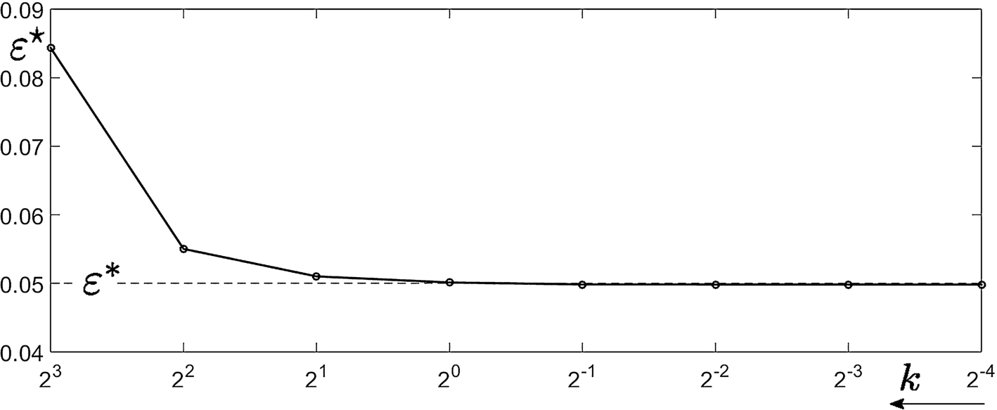
In this example, we first analyze the optimal control $(ξ^{⋆}, α^{⋆})$ for the minimization problem when different values of k are considered. A small set $ω^{*}$ located at $x^{*} = (0, 0)$ , with radius $ε^{*} = 0.05$ , is considered to the construction of the target $z^{m}$ . The information is collected in $Ω_{o} = B_{1} (0) ∖ B_{ρ} (0)$ with $ρ = 0.7$ . In the current setting, we take only one observation by taking into account the Robin data $g^{1}$ . The control was performed by considering $k = 2^{s}$ with $s \in {- 4, - 3, - 2, - 1, 0, 1, 2, 3}$ . The geometrical domain Ω is discretized into 120320 elements comprising 60417 nodes. The combinatorial search was conducted on the sub-mesh of 175 nodes within $Ω ∖ Ω_{o}$ . We successfully find the exact location of the center $x^{*}$ of the set $ω^{*}$ for all values of k. We plot the size of the obtained control $ε^{⋆}$ on vertical axis against the value of k on horizontal axis in Fig. 2. We observe that the exact radius $ε^{*}$ of the control was accurately predicted by $ε^{⋆}$ with $k \in (0, 1]$ , while for $k > 1$ the radius $ε^{*}$ was overestimated. This phenomenon occurs because the parameter k present in topological derivatives and the coefficient α are of similar order in equation (4.5). Hence, we take $k = 1$ for the forthcoming examples. See Remark 2.

Fig. 2.

Example 1: The approximated solution $ε^{⋆}$ for different values of k.

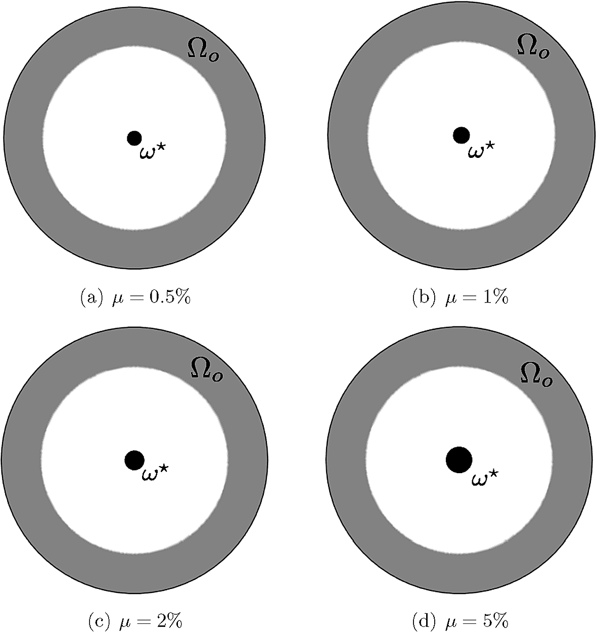
Since the value of k is fixed ( $k = 1$ ), we are now interested in investigating the robustness of the method with respect to noisy data. For this purpose, the measurement $z^{m}$ is corrupted with white Gaussian noise. Therefore, $z^{m} (x)$ is replaced by $z_{μ}^{m} (x) = z^{m} (x) (1 + μ τ (x))$ , where $τ (x)$ is a function assuming random values in the interval $(0, 1)$ and μ corresponds to the noise level. Figure 3 illustrates the optimal control $ω^{⋆}$ for different levels of noise. We successfully find the exact location of the center $x^{*}$ of the set $ω^{*}$ for all noise levels considered. However, the higher is the level of the additive noise, the more overestimated is the size of the obtained optimal control. This statement is confirmed by the quantitative results presented in Table 1.

Table 1

Example 1: Size of the optimal control $ω^{⋆}$ for different values of μ and $M = 1$

	$μ = 0.5 %$	$μ = 1 %$	$μ = 2 %$	$μ = 5 %$
$ε^{⋆}$	0.0574	0.0636	0.0745	0.1

Fig. 3.

Example 1: Results $ω^{⋆}$ .

Fig. 4.

Example 2: $ω^{*} = ω_{1}^{*} \cup ω_{2}^{*}$ .

6.2.2. Example 2

Let the subdomain $Ω_{o}$ be a small circular region centred at $(0.2, 0.2)$ with radius $ρ = 0.3$ in this example. The target $z^{m}$ is constructed by considering a geometrical subdomain $ω^{*}$ consisting of two circular regions, $ω_{1}^{*}$ and $ω_{2}^{*}$ , with radius $ε_{1}^{*} = ε_{2}^{*} = 0.1$ and the centers located at $x_{1}^{*} = (0.4, - 0.5)$ and $x_{2}^{*} = (- 0.5, 0.3)$ , respectively. The domain Ω, subdomain $Ω_{o}$ and the sets $ω_{1}^{*}$ and $ω_{2}^{*}$ are illustrated in Fig. 4. The finite element mesh for the geometrical domain Ω comprises 115712 elements and 58145 nodes. A sub-mesh of 193 points represents the combinatorial search region inside the subdomain $Ω ∖ Ω_{o}$ . Like Example 1, we again consider only one observation with the help of the Robin data $g^{1}$ . By comparing Figs 4 and 5(a), one can observe that the control $ω^{⋆}$ is not satisfactory, since we certainly have $u^{m} \neq {z^{m}}_{|_{Ω_{o}}}$ . This happens because of the lack of information. Therefore, we improve the number of measurements by considering all the Robin data $g^{1}$ , $g^{2}$ and $g^{3}$ simultaneously. Finally, in this case, we obtain the exact centers $x_{1}^{⋆} = x_{1}^{*}$ and $x_{2}^{⋆} = x_{2}^{*}$ . The associated optimal radii were $ε_{1}^{⋆} = 0.10177$ and $ε_{2}^{⋆} = 0.10168$ , which are approximately equal to the true values. Since $ω^{⋆} \approx ω^{*}$ , we have $u^{m} \approx {z^{m}}_{|_{Ω_{o}}}$ and then $ω^{⋆}$ is the optimal control to the problem (6.1). We demonstrate the numerical result in the Fig. 5(b). We conclude by noticing the need of more than one observation in the case of insufficient information. This motivates us to collect data through three boundary excitations $g^{1}$ , $g^{2}$ and $g^{3}$ in the forthcoming example where the sets $ω_{1}^{*}$ and $ω_{2}^{*}$ considered to the construction of the target $z^{m}$ have different sizes.

Fig. 5.

Example 2: Results $ω^{⋆} = ω_{1}^{⋆} \cup ω_{2}^{⋆}$ .

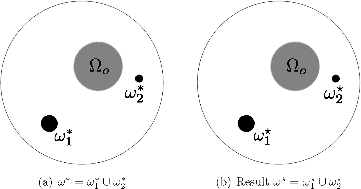
6.2.3. Example 3

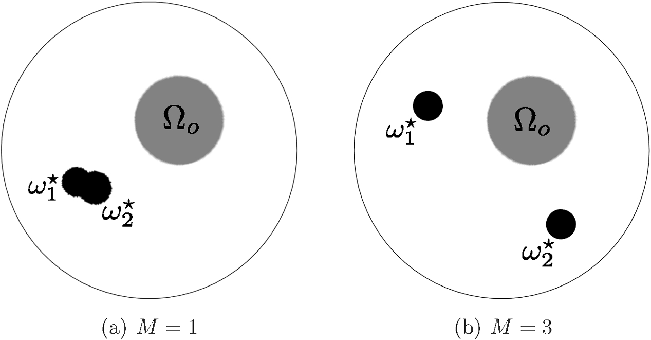
Two circular regions $ω_{1}^{*}$ and $ω_{2}^{*}$ with centers located at $x_{1}^{*} = (- 0.4, - 0.5)$ and $x_{2}^{*} = (0.7, 0)$ with radii $ε_{1}^{*} = 0.1$ and $ε_{2}^{*} = 0.05$ , respectively, are considered to the construction of the target $z^{m}$ . The subdomain $Ω_{o}$ is the same of the previous example. The domain Ω, subdomain $Ω_{o}$ and the sets $ω_{1}^{*}$ and $ω_{2}^{*}$ are illustrated in Fig. 6(a). The geometrical domain Ω is discretized into 142592 elements comprising 71593 nodes. Here, we consider the sub-mesh for the combinatorial search inside the subdomain $Ω ∖ Ω_{o}$ which consists of 245 distributed nodes. Figure 6(b) shows us the optimal control $ω^{⋆}$ . In fact, we obtained the exact centers $x_{1}^{⋆} = x_{1}^{*}$ and $x_{2}^{⋆} = x_{2}^{*}$ ; and the radii $ε_{1}^{⋆} = 0.10313$ and $ε_{2}^{⋆} = 0.04796$ which are approximately equal to the true values $ε_{1}^{*}$ and $ε_{2}^{*}$ , respectively. This example shows us that our proposed algorithm computes the optimal control efficiently in the case of a target constructed from geometrical domains $ω_{1}^{*}$ and $ω_{2}^{*}$ of different sizes.

Fig. 6.

Example 3.

Footnotes

Acknowledgements

This research was partly supported by CNPq (Brazilian Research Council), CAPES (Brazilian Higher Education Staff Training Agency) and FAPERJ (Research Foundation of the State of Rio de Janeiro). These supports are gratefully acknowledged. These research results have also received funding from the EU H2020 Programme and from MCTI/RNP-Brazil under the HPC4E Project, grant agreement n° 689772. The third author would like to thank the Facultad de Ciencias Físicas y Matemáticas, Universidad de Concepción (Chile), for their financial support through PROYECTOS VRID INICIACIÓN n° 216.013.0.41-1.0IN.

References

Ammari,

Garnier,

Jugnon and

Kang, Stability and resolution analysis for a topological derivative based imaging functional, SIAM Journal on Control and Optimization 50(1) (2012), 48–76. doi:10.1137/100812501.

Amstutz, Sensitivity analysis with respect to a local perturbation of the material property, Asymptotic Analysis 49(1–2) (2006), 87–108.

Amstutz and

Andrä, A new algorithm for topology optimization using a level-set method, Journal of Computational Physics 216(2) (2006), 573–588. doi:10.1016/j.jcp.2005.12.015.

Amstutz,

S.M.

Giusti,

A.A.

Novotny and

E.A.

de Souza Neto, Topological derivative for multi-scale linear elasticity models applied to the synthesis of microstructures, International Journal for Numerical Methods in Engineering 84 (2010), 733–756. doi:10.1002/nme.2922.

Amstutz,

A.A.

Novotny and

E.A.

de Souza Neto, Topological derivative-based topology optimization of structures subject to Drucker–Prager stress constraints, Computer Methods in Applied Mechanics and Engineering 233–236 (2012), 123–136. doi:10.1016/j.cma.2012.04.004.

Barbu, Mathematical Methods in Optimization of Differential Systems, Mathematics and Its Applications, Vol. 310, Kluwer Academic Publishers Group, Dordrecht, 1994, Translated and revised from the 1989 Romanian original. doi:10.1007/978-94-011-0760-0.

Bonnet, Higher-order topological sensitivity for 2-D potential problems, International Journal of Solids and Structures 46(11–12) (2009), 2275–2292. doi:10.1016/j.ijsolstr.2009.01.021.

Canelas,

Laurain and

A.A.

Novotny, A new reconstruction method for the inverse potential problem, Journal of Computational Physics 268 (2014), 417–431. doi:10.1016/j.jcp.2013.10.020.

Canelas,

Laurain and

A.A.

Novotny, A new reconstruction method for the inverse source problem from partial boundary measurements, Inverse Problems 31(7) (2015), 075009.

10.

Colton and

Kress, Inverse Acoustic and Electromagnetic Scattering Theory, Springer-Verlag, New York, 1992. doi:10.1007/978-3-662-02835-3.

11.

J.R.

de Faria and

A.A.

Novotny, On the second order topologial asymptotic expansion, Structural and Multidisciplinary Optimization 39(6) (2009), 547–555. doi:10.1007/s00158-009-0436-7.

12.

A.D.

Ferreira and

A.A.

Novotny, A new non-iterative reconstruction method for the electrical impedance tomography problem, Inverse Problems 33(3) (2017), 035005.

13.

Hintermüller and

Laurain, Multiphase image segmentation and modulation recovery based on shape and topological sensitivity, Journal of Mathematical Imaging and Vision 35 (2009), 1–22. doi:10.1007/s10851-009-0150-5.

14.

Hintermüller,

Laurain and

A.A.

Novotny, Second-order topological expansion for electrical impedance tomography, Advances in Computational Mathematics 36(2) (2012), 235–265. doi:10.1007/s10444-011-9205-4.

15.

Isakov, Inverse Problems for Partial Differential Equations, Applied Mathematical Sciences, vol. 127, Springer, New York, 2006.

16.

Isakov,

Leung and

Qian, A fast local level set method for inverse gravimetry, Communications in Computational Physics 10(4) (2011), 1044–1070. doi:10.4208/cicp.100710.021210a.

17.

Kowalewski,

Lasiecka and

Sokołowski, Sensitivity analysis of hyperbolic optimal control problems, Computational Optimization and Applications 52 (2012), 147–179. doi:10.1007/s10589-010-9375-x.

18.

J.-L.

Lions, Optimal Control of Systems Governed by Partial Differential Equations., Die Grundlehren der mathematischen Wissenschaften, Band 170, Springer-Verlag, New York, 1971. Translated from the French by S. K. Mitter. doi:10.1007/978-3-642-65024-6.

19.

J.-L.

Lions, Some Methods in the Mathematical Analysis of Systems and Their Control, Science Press, New York, 1981.

20.

J.-L.

Lions, Contrôlabilité Exacte, Perturbations et Stabilisation de Systèmes Distribués. Tome 1, Recherches en Mathématiques Appliquées [Research in Applied Mathematics], Vol. 8, Masson, Paris, 1988, Contrôlabilité exacte. [Exact controllability], With appendices by E. Zuazua, C. Bardos, G. Lebeau and J. Rauch.

21.

J.-L.

Lions, Contrôlabilité Exacte, Perturbations et Stabilisation de Systèmes Distribués. Tome 2, Recherches en Mathématiques Appliquées [Research in Applied Mathematics], Vol. 9, Masson, Paris, 1988, Perturbations. [Perturbations].

22.

C.G.

Lopes and

A.A.

Novotny, Topology design of compliant mechanisms with stress constraints based on the topological derivative concept, Structural and Multidisciplinary Optimization 54(4) (2016), 737–746. doi:10.1007/s00158-016-1436-z.

23.

C.G.

Lopes,

R.B.

Santos,

A.A.

Novotny and

Sokołowski, Asymptotic analysis of variational inequalities with applications to optimum design in elasticity, Asymptotic Analysis 102 (2017), 227–242. doi:10.3233/ASY-171416.

24.

T.J.

Machado,

J.S.

Angelo and

A.A.

Novotny, A new one-shot pointwise source reconstruction method, Mathematical Methods in the Applied Sciences 40(15) (2017), 1367–1381. doi:10.1002/mma.4059.

25.

J.M.

Melenk, On generalized finite element methods, Ph.D. Thesis, University of Maryland at College Park, Maryland, USA, 1995.

26.

S.A.

Nazarov and

B.A.

Plamenevskij, Elliptic Problems in Domains with Piecewise Smooth Boundaries, de Gruyter Expositions in Mathematics, Vol. 13, Walter de Gruyter & Co., Berlin, 1994. doi:10.1515/9783110848915.

27.

A.A.

Novotny and

Sokołowski, Topological Derivatives in Shape Optimization, Interaction of Mechanics and Mathematics, Springer-Verlag, Berlin, Heidelberg, 2013. doi:10.1007/978-3-642-35245-4.

28.

Osher and

Fedkiw, Level Set Methods and Dynamic Implicit Surfaces, Springer-Verlag, New York, 2003. doi:10.1007/b98879.

29.

Osher and

J.A.

Sethian, Front propagating with curvature dependent speed: Algorithms based on Hamilton–Jacobi formulations, Journal of Computational Physics 79(1) (1988), 12–49. doi:10.1016/0021-9991(88)90002-2.

30.

J.-P.

Raymond, Optimal control of partial differential equations, Institut de Mathématiques, Université Paul Sabatier, 31062 Toulouse Cedex, France, http://www.math.univ-toulouse.fr/~raymond/book-ficus.pdf.

31.

S.S.

Rocha and

A.A.

Novotny, Obstacles reconstruction from partial boundary measurements based on the topological derivative concept, Structural and Multidisciplinary Optimization 55(6) (2017), 2131–2141. doi:10.1007/s00158-016-1632-x.

32.

Samet, Topological sensitivity analysis with respect to a small hole located at the boundary of the domain, Asymptotic Analysis 66(1) (2010), 35–49.

33.

J.A.

Sethian, Level Set Methods and Fast Marching Methods: Evolving Interfaces in Computational Geometry, Fluid Mechanics, Computer Vision, and Materials Science, Cambridge University Press, Cambridge, UK, 1999.

34.

Sokołowski and

Żochowski, On the topological derivative in shape optimization, SIAM Journal on Control and Optimization 37(4) (1999), 1251–1272. doi:10.1137/S0363012997323230.

35.

Sokołowski and

Żochowski, Topological derivative for optimal control problems, Control and Cybernetics 28(3) (1999), 611–626.

36.

Sokołowski and

Żochowski, Modelling of topological derivatives for contact problems, Numerische Mathematik 102(1) (2005), 145–179. doi:10.1007/s00211-005-0635-0.

37.

Sokołowski and

Żochowski, Steklov–Poincaré operator for Helmholtz equation, in: MMAR Proceedings, Miedzyzdroje, Poland, 2015, pp. 728–732.

38.

Van Goethem and

A.A.

Novotny, Crack nucleation sensitivity analysis, Mathematical Methods in the Applied Sciences 33(16) (2010), 1978–1994.

39.

Xavier,

E.A.

Fancello,

J.M.C.

Farias,

Van Goethem and

A.A.

Novotny, Topological derivative-based fracture modelling in brittle materials: A phenomenological approach, Engineering Fracture Mechanics 179 (2017), 13–27. doi:10.1016/j.engfracmech.2017.04.005.

40.

S.E.

Yacoubi and

Sokołowski, Domain optimization problems for parabolic control systems, International Journal of Applied Mathematics and Computer Science 6(2) (1996), 277–289.

Topological asymptotic analysis of an optimal control problem modeled by a coupled system

Abstract

Keywords

1. Introduction

2. Topological derivatives

3. Problem formulation

5.1. Asymptotic development of the cost functional

5.3.1. Estimates for the remainders E ℓ m ( ε ) , ℓ = 1 , … , 10

5.3.2. Estimates for the remainders E ℓ m ( ε ) , ℓ = 11 , … , 19

5.3.3. Estimate for the remainder E 20 m ( ε )

6. Numerical results

6.1. Non-iterative algorithm

6.2. Numerical examples

Footnotes

Acknowledgements

References

5.3.1. Estimates for the remainders $E_{ℓ}^{m} (ε)$ , $ℓ = 1, \dots, 10$

5.3.2. Estimates for the remainders $E_{ℓ}^{m} (ε)$ , $ℓ = 11, \dots, 19$

5.3.3. Estimate for the remainder $E_{20}^{m} (ε)$