Operator estimates for the crushed ice problem

Abstract

Let $Δ_{Ω_{ε}}$ be the Dirichlet Laplacian in the domain $Ω_{ε} : = Ω ∖ (⋃_{i} D_{i ε})$ . Here $Ω \subset R^{n}$ and ${D_{i ε}}_{i}$ is a family of tiny identical holes (“ice pieces”) distributed periodically in $R^{n}$ with period ε. We denote by $cap (D_{i ε})$ the capacity of a single hole. It was known for a long time that $- Δ_{Ω_{ε}}$ converges to the operator $- Δ_{Ω} + q$ in strong resolvent sense provided the limit $q : = {lim}_{ε \to 0} cap (D_{i ε}) ε^{- n}$ exists and is finite. In the current contribution we improve this result deriving estimates for the rate of convergence in terms of operator norms. As an application, we establish the uniform convergence of the corresponding semi-groups and (for bounded Ω) an estimate for the difference of the kth eigenvalue of $- Δ_{Ω_{ε}}$ and $- Δ_{Ω_{ε}} + q$ . Our proofs relies on an abstract scheme for studying the convergence of operators in varying Hilbert spaces developed previously by the second author.

Keywords

Crushed ice problem homogenization norm resolvent convergence operator estimates varying Hilbert spaces

1. Introduction

In the current work we revisit one of the classical problems in homogenization theory – homogenization of the Dirichlet Laplacian in a domain with a lot of tiny holes. It is also known as crushed ice problem. Below, we briefly recall the setting of this problem and the main result.

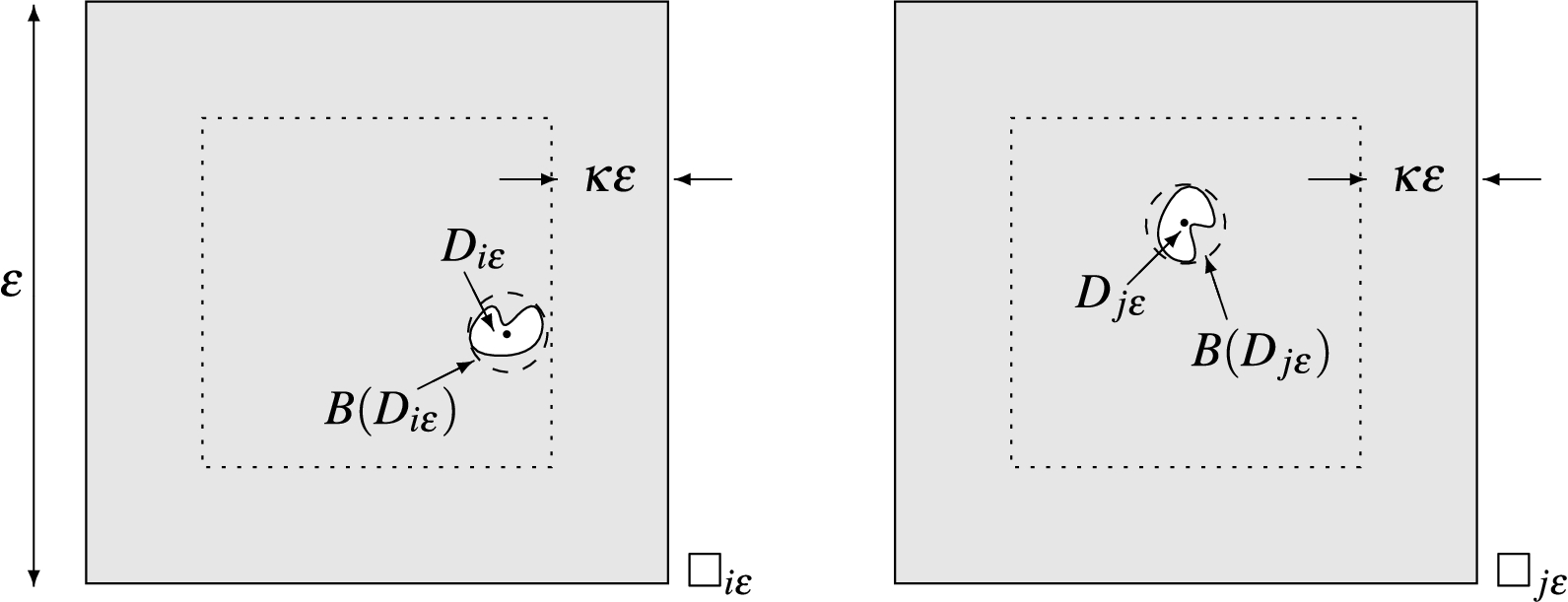
Let Ω be an open domain in $R^{n}$ ( $n ⩾ 2$ ) and ${D_{i ε}}_{i}$ be a family of small holes. The holes are identical (up to a rigid motion) and are distributed evenly in Ω along the ε-periodic cubic lattice – see Fig. 1. We set $\begin{array}{l} Ω_{ε} : = Ω ∖ (⋃_{i} \overline{D_{i ε}}) . \end{array}$ The domain $Ω_{ε}$ is depicted in Fig. 1. More precise description of this domain will be given in the next section.

Fig. 1.

The domain $Ω_{ε}$ obtained from Ω by removing the obstacles $D_{i ε}$ . To avoid technical problems with the boundary of Ω, the obstacles are only placed into cells which lie entirely in Ω.

In $Ω_{ε}$ we study the following problem: $\begin{array}{l} - Δ_{Ω_{ε}} u_{ε} + u_{ε} = f ↾_{Ω_{ε}}, \end{array}$ where $Δ_{Ω_{ε}}$ is the Dirichlet Laplacian in $Ω_{ε}$ , $f \in L_{2} (Ω)$ is a given function, $f ↾_{Ω_{ε}}$ is the restriction of f to $Ω_{ε}$ . The goal is to describe the behaviour of the solution $u_{ε}$ to this problem as $ε \to 0$ .

It turns out that the result depends on the limit $q : = {lim}_{ε \to 0} cap (D_{i ε}) ε^{- n}$ being finite or infinite (here $cap (D_{i ε})$ is the capacity of a single hole, see (8) for details). Namely, if $q = \infty$ then $‖ u_{ε} ‖_{L_{2} (Ω_{ε})} \to 0$ as $ε \to 0$ . Otherwise, if $q < \infty$ , $‖ u_{ε} - u ‖_{L_{2} (Ω_{ε})} \to 0$ as $ε \to 0$ , where u is the solution to the problem $\begin{matrix} - Δ_{Ω} u + q u + u = f . \end{matrix}$ This result was proven independently by V.A. Marchenko, E.Ya. Khruslov [27] (the case $q < \infty$ ), J. Rauch, M. Taylor [37] (the cases $q = 0$ and $q = \infty$ ) and D. Cioranescu, F. Murat [16] (all scenario) by using different tools – potential theory, capacitary methods and variational approach (the so-called Tartar’s energy method), respectively. J. Rauch and M. Taylor also treated the case of randomly distributed holes under assumptions resembling the case $q > 0$ in a deterministic case; the pioneer result in this direction was obtained by M. Kac in [23], who investigated the case of uniformly distributed holes.

Note, that this result remains valid if on the external boundary (i.e. on $\partial Ω ∖ (⋃_{i} \partial D_{i ε})$ ) one imposes Neumann, Robin, mixed or any other ε-independent boundary conditions (then $- Δ_{Ω}$ is the Laplace operator subject to these conditions on $\partial Ω$ ).

Besides the resolvent convergence one can study the convergence of the spectrum or the convergence of the semi-group $exp (Δ_{Ω_{ε}} t)$ . In the later case the name crushed ice problem is indeed reasonable.1

Let us assume that Ω is an isolated container occupied by a homogeneous medium, while the sets $D_{i ε}$ are regarded as a small pieces of ice. Under a certain idealization (the ice pieces do not melt and move) the heat distribution in $Ω_{ε}$ at time $t > 0$ is described by the function $exp (Δ_{Ω_{ε}} t) u_{0}$ , where $Δ_{Ω_{ε}}$ is the Laplace operator subject to Dirichlet conditions on the boundary of the ice pieces and Neumann conditions on $\partial Ω$ (since the container is isolated), $u_{0}$ is the heat distribution at $t = 0$ .

Also domains with a lot of Dirichlet holes have interesting scattering properties (fading/solidifying obstacles, cf. [36,37]).

For more details on the topic we refer also to articles [3,5,25,31,32,35], as well as to the monographs [11,13,14,28,29,38].

In what follows, we focus on the case $q < \infty$ .

In the language of operator theory one can reformulate the above result as follows: the operator $- Δ_{Ω_{ε}}$ converges to the operator $- Δ_{Ω} + q$ in strong resolvent sense. Strictly speaking, we are not able to treat the classical resolvent convergence (since the underlying operators act in different Hilbert spaces), but we have its natural analogue for varying domains with $Ω_{ε} \subset Ω$ : $\begin{array}{l} (1) & \forall f \in L_{2} (Ω) : {‖ {(- Δ_{Ω_{ε}} + I)}^{- 1} J_{ε} f - J_{ε} {(- Δ_{Ω} + q + I)}^{- 1} f ‖}_{L_{2} (Ω_{ε})} \to 0 as ε \to 0, \end{array}$ where $J_{ε} f : = f ↾_{Ω_{ε}}$ .

In the recent work [17] the authors improved (1) by proving (a kind of) norm resolvent convergence, namely $\begin{array}{l} (2) & {‖ J_{ε}^{'} {(- Δ_{Ω_{ε}} + I)}^{- 1} - {(- Δ_{Ω} + q + I)}^{- 1} J_{ε}^{'} ‖}_{L (L_{2} (Ω_{ε}), L_{2} (Ω))} \to 0 as ε \to 0, \end{array}$ where $J_{ε}^{'} : L_{2} (Ω_{ε}) \to L_{2} (Ω)$ is the operator of extension by zero. The authors assumed that $D_{i ε}$ are balls, distributed ε-periodically in Ω. For bounded Ω their proof resembles the variational approach developed in [16], for unbounded Ω they also utilize a rapid decay of the Green’s function of $- Δ + I$ .

In the current work we extend the result of [17] providing an estimate for the rate of convergence in (2) (see Theorem 2.5 below). We also improve (1) (see Theorem 2.3) deriving the operator estimate $\begin{array}{l} {‖ {(- Δ_{Ω_{ε}} + I)}^{- 1} J_{ε} - J_{ε} {(- Δ_{Ω} + q + I)}^{- 1} ‖}_{L (L_{2} (Ω), L_{2} (Ω_{ε}))} ⩽ 4 δ_{ε}, \end{array}$ where $δ_{ε} = | q - {lim}_{ε \to 0} cap (D_{ε}) ε^{- n} | + γ_{ε}$ with $γ_{ε} = o (1)$ depending on the dimension n (for the “physical” cases $n = 2$ and $n = 3$ one has $γ_{ε} = O (ε ln ε)$ and $γ_{ε} = O (ε)$ , respectively).

As a consequence of our main results, we establish uniform convergence of the corresponding semi-groups and (for bounded Ω) an estimate for the difference between the kth eigenvalue of $- Δ_{Ω_{ε}}$ and $- Δ_{Ω} + q$ – see Theorems 2.6–2.7.

Let us stress that in all our results (except Theorem 2.7) we do not assume that the domain Ω is bounded.

Our proofs are based on the abstract scheme for studying the convergence of operators in varying Hilbert spaces which was developed by the second author of the present article in [33] and in more detail in the monograph [34].

Before proceeding to the main part of the work let us mention several related results:

Some estimates for the rate of convergence in (1) were obtained in [14, §16]. Namely, assuming that $n = 3$ , $D_{i ε}$ are balls of radius $ε^{3}$ (that is $cap (D_{i ε}) ε^{- 3} = 4 π = q$ ) distributed ε-periodically, and the function f belongs to the Hölder class $C^{0, a} (\overline{Ω})$ , the authors derived the estimates $\begin{array}{l} {‖ {(- Δ_{Ω_{ε}} + I)}^{- 1} J_{ε} f - J_{ε} {(- Δ_{Ω} + q + I)}^{- 1} f ‖}_{L_{2} (Ω_{ε})} ⩽ C ε ‖ f ‖_{C^{0, a} (\overline{Ω})}, \\ (3) & {‖ {(- Δ_{Ω_{ε}} + I)}^{- 1} J_{ε} f - J_{ε} φ_{ε} {(- Δ_{Ω} + q + I)}^{- 1} f ‖}_{H^{1} (Ω_{ε})} ⩽ C ε ‖ f ‖_{C^{0, a} (\overline{Ω})}, \end{array}$ where $φ_{ε}$ is the operator of multiplication by a certain cut-off function.

(3)-like estimates were also obtained in [5]. In this work the holes are distributed ε-periodically in a bounded domain $Ω \subset R^{n}$ ( $n ⩾ 2$ ), no special assumptions on the geometry of holes are imposed. Let $f \in L_{\infty} (Ω)$ . Then one has the estimate $\begin{array}{l} {‖ {(- Δ_{Ω_{ε}})}^{- 1} J_{ε} f - J_{ε} ψ_{ε} {(- Δ_{Ω} + q)}^{- 1} f ‖}_{H^{1} (Ω_{ε})} ⩽ Λ_{ε} ‖ f ‖_{L_{\infty} (Ω)}, lim_{ε \to 0} Λ_{ε} = 0, \end{array}$ where the small factor $Λ_{ε}$ is expressed in terms of the first eigenvalue of the Laplace operator on a period cell subject to the Dirichlet conditions on the hole boundary and the periodic conditions on the external part of the period cell boundary; the function $ψ_{ε}$ is built on the basis of the corresponding eigenfunction.

One can also study a surface distribution of holes, i.e. holes being located near some hypersurface Γ intersecting Ω. This problem was first considered in [27]; it was proved that the limit operator is $- Δ_{Ω} + q δ_{Γ}$ . Here $q \in L_{\infty} (Γ)$ is a positive function, and $δ_{Γ}$ is a delta-distribution supported on Γ. For the case $n = 2$ , the norm resolvent convergence with estimates on the rate of convergence were obtained in [9], where even more general elliptic operators were treated. The proofs in [9] rely on variational formulations for the pre-limit and the homogenized resolvent equations (the key object of their analysis is a certain integral identity associated with the difference of the resolvents). Note that the method we use in the current works allows to treat surface distributions of holes as well. Nevertheless, to simplify the presentation, we focus on the bulk distribution of holes only.

Operator estimates in homogenization theory is a rather young topic. The classical homogenization problem concerning elliptic operators of the form $\begin{array}{l} A_{ε} = - div (A (\frac{.}{ε}) \nabla), where A (\cdot) is a Z^{n} -periodic function, \end{array}$ was first treated in [6,7,19,20,42–44], see the recent papers [39,45] for further references. In particular, the article [43] deals with a perturbation which is defined by rescaling an abstract periodic measure. The technique developed in [43] can be applied for deriving operator estimates is the case of periodically perforated domains provided the sizes of holes and distances between them are of the same smallness order (evidently, this does not hold for the problem we study in the current paper). Operator estimates were also obtained for elliptic operators with frequently alternating boundary conditions (see, e.g., [8]), for problems in domains with oscillating boundary [10], or for the “double-porosity” model in [15]. For more results we refer to the paper [9] containing a comprehensive overview on operator estimates in homogenization theory.

In [2] we treat (possibly non-compact) manifolds with an increasing (even infinite) number of balls removed (similarly as in [37]), and show operator estimates using similar methods as in this article.

2. Setting of the problem and main results

Let $n ⩾ 2$ and let $Ω \subset R^{n}$ be a domain (not necessarily bounded) with $C^{2}$ -boundary $\partial Ω$ . We also assume that there exists a constant $θ_{Ω} > 0$ such that the following map is injective on $\partial Ω \times [0, θ]$ provided $θ < θ_{Ω}$ : $\begin{array}{l} (4) & (x, t) \mapsto x + t ν (x), \end{array}$ where $ν : \partial Ω \to S^{n - 1}$ the unit inward-pointing normal vector field on $\partial Ω$ .

Additionally, we require Ω to be uniformly regular in the sense of Browder [12]. This requirement is automatically fulfilled, for example, for domains with compact smooth boundaries or for compact, smooth perturbations of half-spaces. Under this assumption the Dirichlet Laplacian in Ω defined via $\begin{matrix} dom (Δ_{Ω}) = H^{2} (Ω) \cap H_{0}^{1} (Ω), Δ_{Ω} f : = Δ f \end{matrix}$ is a self-adjoint operator (see, e.g., the recent paper [4] for more details and references on this issue).

We note, that our results remain valid under less restrictive assumptions on $\partial Ω$ , see Remark 4.8 below.

In what follows we denote by C, $C_{1}$ etc. generic constants depending only on the dimension n.

We set $□ : = {(- 1 / 2, 1 / 2)}^{n}$ .

Now we describe a family of holes in Ω (see Fig. 2). Let $D_{ε}$ be a Lipschitz domain in $R^{n}$ depending on a small parameter $ε > 0$ . We denote by $d_{ε}$ the radius of the smallest ball containing $D_{ε}$ . It is assumed that $\begin{array}{l} (5) & {(d_{ε})}^{n - 2} ⩽ C ε^{n} as n ⩾ 3, | ln d_{ε} |^{- 1} ⩽ C ε^{2} as n = 2, or \\ d_{ε} ⩽ \{\begin{matrix} C_{1} ε^{n / (n - 2)} & as n ⩾ 3, \\ exp (- 1 / (C ε^{2})) & as n = 2 \end{matrix} \end{array}$ (hence, in particular, $d_{ε} = o (ε)$ ). For $i \in Z^{n}$ , let $D_{i ε}$ be a set enjoying the following properties: $\begin{array}{l} D_{i ε} coincides with D_{ε} up to a rigid motion, \\ B (D_{i ε}) \subset □_{i ε} : = ε (□ + i), \\ (6) & dist (B (D_{i ε}), \partial □_{i ε}) ⩾ κ ε for some κ > 0, \end{array}$ where $B (D_{i ε})$ is the smallest ball containing $D_{i ε}$ (the radius of this ball is $d_{ε}$ ).

Fig. 2.

Two scaled cells $□_{i ε}$ and $□_{j ε}$ and possible positions of the obstacles $D_{i ε}$ and $D_{j ε}$ (white). The smallest ball $B (D_{i ε})$ (dashed circle) containing the obstacle $D_{i ε}$ has security distance $κ ε$ from the boundary of $□_{i ε}$ , i.e., it should stay inside the dotted cube of side length $(1 - 2 κ) ε$ .

Finally, we set $\begin{array}{l} Ω_{ε} : = Ω ∖ (⋃_{i \in I_{ε}} \overline{D_{i ε}}), \end{array}$ where $\begin{array}{l} I_{ε} : = {i \in Z^{n} : □_{i ε} \subset Ω}, \end{array}$ i.e. the set of those indices for which the rescaled unit cell $□_{i ε}$ is entirely in Ω (with positive distance to $\partial Ω$ ). The domain $Ω_{ε}$ is depicted in Fig. 1.

By $A_{ε}$ we denote the Dirichlet Laplacian on $Ω_{ε}$ , i.e. the operator acting in the Hilbert space $L_{2} (Ω_{ε})$ associated with the closed densely defined positive sesquilinear form $\begin{array}{l} a_{ε} [u, v] : = \int_{Ω_{ε}} \nabla u \cdot \nabla \bar{v} d x, dom (a_{ε}) : = H_{0}^{1} (Ω_{ε}) . \end{array}$

Our goal is to describe the behaviour of the resolvent ${(A_{ε} + I)}^{- 1}$ as $ε \to 0$ under the assumption that the following limit exists and is finite: $\begin{array}{l} (7) & q = lim_{ε \to 0} \frac{cap (D_{ε})}{ε^{n}}, \end{array}$ where $cap (D_{ε})$ is the capacity of the set $D_{ε}$ . Recall (see, e.g., [40]), that for $n ⩾ 3$ the capacity of a set $D \subset R^{n}$ is defined via $\begin{array}{l} (8) & cap (D) = \int_{R^{n}} {| \nabla H (x) |}^{2} d x, \end{array}$ where H is a solution to the problem $\begin{array}{l} (9) & \{\begin{matrix} Δ H (x) = 0, & x \in R^{n} ∖ \overline{D}, \\ H (x) = 1, & x \in \partial D, \\ H (x) \to 0, & | x | \to \infty . \end{matrix} \end{array}$ One has also the following variational characterization of the capacity, namely $\begin{array}{l} (10) & cap (D) = inf \int_{R^{n}} {| \nabla u (x) |}^{2} d x, \end{array}$ where the infimum is taken over $u \in C_{0}^{\infty} (R^{n})$ being equal to 1 on a neighbourhood of D.

For $n = 2$ the right-hand-side of (10) is zero for an arbitrary domain D, hence we need a modified definition. It is as follows: $\begin{array}{l} (11) & cap (D) = \int_{B_{1}} {| \nabla H (x) |}^{2} d x, \end{array}$ where $B_{1}$ is the unit ball concentric with $B (D)$ – the smallest ball containing D (here we assume that the set D is small enough so that $D \subset B (D) \subset B_{1}$ ), H solves the problem $\begin{array}{l} (12) & \{\begin{matrix} Δ H (x) = 0, & x \in B_{1} ∖ \overline{D}, \\ H (x) = 1, & x \in \partial D, \\ H (x) = 0, & x \in \partial B_{1} . \end{matrix} \end{array}$

Further, proving the main results, we will use the following pointwise estimates for the functions H at some positive distance from $B (D)$ , see [29, Lemma 2.4].

Lemma 2.1.

Let $x \in R^{n} ∖ \overline{B (D)}$ . We denote by $ρ (x)$ the distance from x to $B (D)$ , and by d the radius of $B (D)$ . One has: $\begin{array}{l} | H (x) | ⩽ \frac{C \cdot d^{n - 2}}{{(ρ (x))}^{n - 2}}, | \nabla H (x) | ⩽ \frac{C \cdot d^{n - 2}}{{(ρ (x))}^{n - 1}} as n ⩾ 3, \\ | H (x) | ⩽ \frac{C | ln d |^{- 1}}{| ln ρ (x) |^{- 1}}, | \nabla H (x) | ⩽ \frac{C | ln d |^{- 1}}{ρ (x)} as n = 2 \end{array}$ provided $ρ (x) ⩾ C_{0} d$ as $n ⩾ 3$ or $ρ (x) ⩾ exp (- C_{0} \sqrt{| ln d |})$ as $n ⩾ 3$ , for some $C_{0} > 0$ .

Remark 2.2.

Due to (7) one has $\begin{array}{l} (13) & cap (D_{ε}) ε^{- n} = O (1) . \end{array}$ In fact, this condition also follows directly from (5). Indeed, using the monotonicity of the capacity, we get $cap (D_{ε}) ⩽ cap (B_{ε})$ , where $B_{ε}$ is ball of radius $d_{ε}$ containing $D_{ε}$ . For this ball the function H can be computed explicitly: $\begin{matrix} H (x) = \frac{{(d_{ε})}^{n - 2}}{| x |^{n - 2}} as n ⩾ 3, H (x) = \frac{ln x}{ln d_{ε}} as n = 2, \end{matrix}$ hence $cap (B_{ε}) = (n - 2) | S^{n - 1} | {(d_{ε})}^{n - 2}$ as $n ⩾ 3$ and $cap (B_{ε}) = 2 π | ln d_{ε} |^{- 1}$ as $n = 2$ , hence, due to (5), we get (13).

Finally, we introduce the limiting operator $A$ . It acts in $L_{2} (Ω)$ and is defined by $\begin{matrix} A : = - Δ_{Ω} + q I, dom (A) : = dom (Δ_{Ω}) = H^{2} (Ω) \cap H_{0}^{1} (Ω) \end{matrix}$ (recall, that q is defined by (7)). By $a$ we denote the associated form: $\begin{array}{l} a [u, v] : = \int_{Ω} (\nabla u \cdot \nabla \bar{v} + q u \bar{v}) d x, dom (a) : = H_{0}^{1} (Ω) . \end{array}$

The operators $A_{ε}$ and $A$ act in different Hilbert spaces, namely $H_{ε} : = L_{2} (Ω_{ε})$ and $H : = L_{2} (Ω)$ , respectively. Therefore we are not able to apply the usual notion of resolvent convergence and thus a suitable modification is needed. There are many ways how to do this in a “smart” way. For example (cf. [22,41]), one can treat the behaviour of the operator $\begin{matrix} {(A_{ε} + I)}^{- 1} J_{ε} - J_{ε} {(A + I)}^{- 1} \in L (H, H_{ε}), \end{matrix}$ where $J_{ε} : H \to H_{ε}$ is a suitable bounded linear operator satisfying $\begin{array}{l} (14) & \forall f \in H : ‖ J_{ε} f ‖_{H_{ε}} \to ‖ f ‖_{H} as ε \to 0 . \end{array}$

It is natural to choose the operator $J_{ε}$ as the operator of restriction to $Ω_{ε}$ , i.e. $\begin{array}{l} (15) & (J_{ε} f) (x) = \{\begin{matrix} f (x), & x \in Ω_{ε}, \\ 0, & x \in ⋃_{i \in I_{ε}} D_{i ε} . \end{matrix} \end{array}$ Due to (5) one has for each compact set $K \subset R^{n}$ $\begin{array}{l} (16) & \sum_{i : D_{i ε} \subset K} | D_{i ε} | ⩽ α_{ε} | K |, α_{ε} = o (1) does not depend on K, \end{array}$ where $| K |$ stands for the Lebesgue measure of K. Hence, evidently, (14) holds. The results of [16,27,37] can be reformulated as follows: $\begin{matrix} \forall f \in H : lim_{ε \to 0} {‖ {(A_{ε} + I)}^{- 1} J_{ε} f - J_{ε} {(A + I)}^{- 1} f ‖}_{H_{ε}} \to 0, \end{matrix}$ i.e. one has a kind of strong resolvent convergence.

Now, we can state our main result.

Theorem 2.3.

One has $\begin{array}{l} {‖ {(A_{ε} + I)}^{- 1} J_{ε} - J_{ε} {(A + I)}^{- 1} ‖}_{L (H, H_{ε})} ⩽ 4 δ_{ε}, \end{array}$ where $δ_{ε}$ is defined by $\begin{array}{l} (17) & δ_{ε} = | cap (D_{ε}) ε^{- n} - q | + C_{Ω, κ, β} \cdot \{\begin{matrix} ε | ln ε |, & n = 2, \\ ε, & n = 3 \\ ε^{1 - β}, β > 0, & n = 4, \\ max {ε; d_{ε} ε^{- 1}}, & n ⩾ 5, \end{matrix} \end{array}$ and the constant $C_{Ω, κ, β}$ depends on the domain Ω, the relative distance κ of the obstacles from the period cell boundary (see ( 6 )), and, in the case $n = 4$ , on β.

Remark 2.4.

Via the same arguments as in Remark 2.2 one gets ${(d_{ε})}^{n - 2} ε^{- n} ⩾ C > 0$ provided $q > 0$ , hence, using the definition of $δ_{ε}$ , we obtain $\begin{matrix} q > 0, n ⩾ 5 : δ_{ε} = | cap (D_{ε}) ε^{- n} - q | + C_{Ω, κ} ε^{2 / (n - 2)} . \end{matrix}$

Let $J_{ε}^{'} : H_{ε} \to H$ be the operator of extension by zero: $\begin{array}{l} (18) & (J_{ε}^{'} u) (x) = \{\begin{matrix} u (x), & x \in Ω_{ε}, \\ 0, & x \in ⋃_{i \in I_{ε}} D_{i ε} . \end{matrix} \end{array}$ Then the main result of [17] is equivalent to $\begin{matrix} {‖ J_{ε}^{'} {(A_{ε} + I)}^{- 1} - {(A + I)}^{- 1} J_{ε}^{'} ‖}_{L (H_{ε}, H)} \to 0, ε \to 0 . \end{matrix}$ The next theorem gives an improvement of this statement.

Theorem 2.5.

One has $\begin{array}{l} {‖ J_{ε}^{'} {(A_{ε} + I)}^{- 1} - {(A + I)}^{- 1} J_{ε}^{'} ‖}_{L (H_{ε}, H)} ⩽ 6 δ_{ε}, \end{array}$ where $δ_{ε}$ is defined in ( 17 ). Moreover, $\begin{array}{l} {‖ J_{ε}^{'} {(A_{ε} + I)}^{- 1} J_{ε} - {(A + I)}^{- 1} ‖}_{L (H, H)} ⩽ 9 δ_{ε}, \\ {‖ {(A_{ε} + I)}^{- 1} - J_{ε} {(A + I)}^{- 1} J_{ε}^{'} ‖}_{L (H_{ε}, H_{ε})} ⩽ 13 δ_{ε} . \end{array}$

One important applications of the norm resolvent convergence is the uniform convergence of semi-groups generated by $A_{ε}$ and $A$ . Namely, we can approximate $exp (- A_{ε} t)$ in terms of simpler operators $exp (- A t)$ , $J_{ε}$ and $J_{ε}^{'}$ :

Theorem 2.6.

One has for each $t > 0$ : $\begin{matrix} {‖ exp (- A_{ε} t) - J_{ε} exp (- A t) J_{ε}^{'} ‖}_{L (H_{ε}, H_{ε})} ⩽ c_{t} δ_{ε}, \end{matrix}$ where $δ_{ε}$ is defined in ( 17 ), and the constant $c_{t}$ depends only on t.

Another important application is the Hausdorff convergence of spectra, see [17]. Using Theorem 2.3 we are able to extend this result by obtaining an estimate for the difference between the corresponding eigenvalues. Namely, let the domain Ω be bounded. We denote by ${λ_{k, ε}}_{k \in N}$ and ${λ_{k}}_{k \in N}$ the sequences of the eigenvalues of $A_{ε}$ and $A$ , respectively, arranged in the ascending order and repeated according to their multiplicities.

Theorem 2.7.

For each $k \in N$ one has $\begin{matrix} (19) & lim_{ε \to 0} λ_{k, ε} = λ_{k}, \end{matrix}$ moreover $\begin{matrix} (20) & | λ_{k, ε} - λ_{k} | ⩽ 4 C_{ε} (λ_{k, ε} + 1) (λ_{k} + 1) δ_{ε}, \end{matrix}$ where $δ_{ε}$ is defined in ( 17 ), and $| C_{ε} | ⩽ C$ , ${lim}_{ε \to 0} C_{ε} = 1$ .

In the next section we introduce an abstract scheme, which then will be applied for the proof of the above theorems.

3. Abstract framework

In this section we present an abstract scheme for studying the convergence of operators in varying Hilbert spaces. It was developed by the second author of the present article in [33] and in more detail in the monograph [34] (see also the later work [30], where non-self-adjoint operators were treated).

Let $H$ and $H_{ε}$ be two separable Hilbert spaces. Note, that within this section $H_{ε}$ is just a notation for some Hilbert space, which (in general) differs from the space $H$ , i.e. the sub-index ε does not mean that this space depends on a small parameter. Of course, further we will use the results of this section for the ε-dependent space $H_{ε} = L_{2} (Ω_{ε})$ .

Let $a$ and $a_{ε}$ be closed, densely defined, non-negative sesquilinear forms in $H$ and $H_{ε}$ , respectively. We denote by $A$ and $A_{ε}$ the non-negative, self-adjoint operators associated with $a$ and $a_{ε}$ , respectively.

Associated with the operator $A$ , we can introduce a natural scale of Hilbert spaces $H^{k}$ defined via the abstract Sobolev norm: $\begin{array}{l} H^{k} = dom A^{k / 2}, ‖ f ‖_{H^{k}} : = ‖ f ‖_{k} : = {‖ {(A + I)}^{k / 2} f ‖}_{H} . \end{array}$ In particular, we have $H^{0} = H$ with $‖ f ‖_{H^{0}} = ‖ f ‖_{H}$ , $H^{1} = dom (a)$ with $‖ f ‖_{H^{1}} = {(a [f, f] + ‖ f ‖_{H}^{2})}^{1 / 2}$ , and $H^{2} = dom (A)$ with $‖ f ‖_{H^{2}} = ‖ A f + f ‖_{H}$ .

Similarly, we denote by $H_{ε}^{k}$ the scale of Hilbert spaces associated with $A_{ε}$ . The corresponding norms will be denoted by $‖ \cdot ‖_{H_{ε}^{k}}$ .

We now need pairs of so-called identification or transplantation operators acting on the Hilbert spaces and later also pairs of identification operators acting on the form domains.

Definition 3.1 (See [33, App.] or [34, Ch. 4]).

Let $δ_{ε} ⩾ 0$ and $k \in N$ . Moreover, let $J_{ε} : H \to H_{ε}$ and $J_{ε}^{'} : H_{ε} \to H$ be linear bounded operators. In addition, let $J_{ε}^{1} : H^{1} \to H_{ε}^{1}$ and $J_{ε}^{1'} : H_{ε}^{1} \to H^{1}$ be linear bounded operators on the form domains. We say that $(H, a)$ and $(H_{ε}, a_{ε})$ are $δ_{ε}$ -close of order k with respect to the operators $J_{ε}$ , $J_{ε}^{'}$ , $J_{ε}^{1}$ , $J_{ε}^{1'}$ , if the following conditions hold: $\begin{array}{l} (C_{1 a}) & {‖ J_{ε} f - J_{ε}^{1} f ‖}_{H_{ε}} ⩽ δ_{ε} ‖ f ‖_{H^{1}}, \forall f \in H^{1}, \\ (C_{1 b}) & {‖ J_{ε}^{'} u - J_{ε}^{1'} u ‖}_{H} ⩽ δ_{ε} ‖ u ‖_{H_{ε}^{1}}, \forall u \in H_{ε}^{1}, \\ (C_{2}) & | {(J_{ε} f, u)}_{H_{ε}} - {(f, J_{ε}^{'} u)}_{H} | ⩽ δ_{ε} ‖ f ‖_{H} ‖ u ‖_{H_{ε}}, \forall f \in H, u \in H_{ε}, \\ (C_{3 a}) & ‖ J_{ε} f ‖_{H_{ε}} ⩽ (1 + δ_{ε}) ‖ f ‖_{H}, \forall f \in H, \\ (C_{3 b}) & {‖ J_{ε}^{'} u ‖}_{H} ⩽ (1 + δ_{ε}) ‖ u ‖_{H_{ε}}, \forall u \in H_{ε}, \\ (C_{4 a}) & {‖ f - J_{ε}^{'} J_{ε} f ‖}_{H} ⩽ δ_{ε} ‖ f ‖_{H^{1}}, \forall f \in H^{1}, \\ (C_{4 b}) & {‖ u - J_{ε} J_{ε}^{'} u ‖}_{H_{ε}} ⩽ δ_{ε} ‖ u ‖_{H_{ε}^{1}}, \forall u \in H_{ε}^{1}, \\ (C_{5}) & | a_{ε} (J_{ε}^{1} f, u) - a (f, J_{ε}^{1'} u) | ⩽ δ_{ε} ‖ f ‖_{H^{k}} ‖ u ‖_{H_{ε}^{1}}, \forall f \in H^{k}, u \in H_{ε}^{1} . \end{array}$

Remark 3.2.
For $δ_{ε} = 0$ the definition above implies that the operators $A$ and $A_{ε}$ are unitary equivalent. Indeed, ( C 2 )–( C 4 b ) assure that the operator $J_{ε}$ is unitary with the inverse $J_{ε}^{'}$ ; due to ( C 1 a )–( C 1 b ) $J_{ε}^{1}$ and $J_{ε}^{1'}$ are the restrictions of $J_{ε}$ and $J_{ε}^{1}$ onto $dom (a)$ and $dom (a_{ε})$ , respectively. Hence, in view of ( C 5 ), $J_{ε}$ realises the unitary equivalence of $A$ and $A_{ε}$ .

Now, we present the main implications of the definition of $δ_{ε}$ -closeness.
Theorem 3.3 ([33, Th. A.5]).

One has $\begin{array}{l} {‖ {(A_{ε} + I)}^{- 1} J_{ε} - J_{ε} {(A + I)}^{- 1} ‖}_{L (H, H_{ε})} ⩽ 4 δ_{ε}, \end{array}$ provided conditions ( C 1 a ), ( C 1 b ), ( C 2 ), and ( C 5 ) hold with $k ⩽ 2$ .

Remark 3.4.
Let $A_{ε}$ ( $ε > 0$ ), $A$ be non-negative self-adjoint operators in the same Hilbert space $H$ , and let $a_{ε}$ and $a$ be the corresponding sesquilinear forms. We assume that $dom (a_{ε}) = dom (a)$ and $\begin{array}{l} (21) & | a_{ε} (f, u) - a (f, u) | ⩽ δ_{ε} \sqrt{a [f, f] + ‖ f ‖_{H}} \sqrt{a_{ε} [u, u] + ‖ u ‖_{H}}, \forall f, u \in dom (a), \end{array}$ where $δ_{ε} \to 0$ as $ε \to 0$ . Due to (21) $(H, a)$ and $(H, a_{ε})$ are $δ_{ε}$ -close of order 1 with respect to the identity maps $J_{ε}$ , $J_{ε}^{'}$ (on $H$ ) and $J_{ε}^{1}$ , $J_{ε}^{1'}$ (on $dom (a)$ ). Then by Theorem 3.3 $\begin{array}{l} (22) & {‖ {(A_{ε} + I)}^{- 1} - {(A + I)}^{- 1} ‖}_{L (H)} \to 0 . \end{array}$ In fact, it would suffice for (22) if (21) is satisfied whenever $f = u$ , see Theorem VI.3.6 in T. Kato’s monograph [24]. In this sense, Theorem 3.3 can be regarded as a generalization of this classical result to the setting of varying spaces.
Theorem 3.5 ([33, Th. A.8]).

Let $U \subset \overline{R_{+}}$ be an open set containing either $σ (A)$ or $σ (A_{ε})$ . Let $ψ : \overline{R_{+}} \to C$ be a bounded measurable function, continuous on U and such that the limit ${lim}_{λ \to \infty} ψ (λ)$ exists.

Then there exists $η_{ψ} (δ) > 0$ with $η_{ψ} (δ) \to 0$ as $δ \to 0$ such that $\begin{array}{l} (23) & {‖ ψ (A_{ε}) J_{ε} - J_{ε} ψ (A) ‖}_{L (H, H_{ε})} ⩽ η_{ψ} (δ_{ε}) \end{array}$ for all pairs $(H, a)$ and $(H_{ε}, a_{ε})$ , which are $δ_{ε}$ -close of order $k ⩽ 2$ .

Remark 3.6.
The important example of the function ψ satisfying the requirements of the above theorem is $ψ (λ) = exp (- λ t)$ , $t > 0$ is a parameter. Another important example is the function $ψ = 1_{(α, β)}$ – the characteristic function of the interval $(α, β)$ with $α, β \notin σ (A)$ or $α, β \notin σ (A_{ε})$ . In this case Theorem 3.5 gives the closeness of the spectral projections.
Theorem 3.7 ([33, Th. A.10]).

Let for some function ψ the estimate ( 23 ) be valid. Then $\begin{array}{l} {‖ J_{ε}^{'} ψ (A_{ε}) - ψ (A) J_{ε}^{'} ‖}_{L (H_{ε}, H)} ⩽ η_{ψ} (δ_{ε}) + 2 ‖ ψ ‖_{\infty} δ_{ε}, \\ {‖ J_{ε}^{'} ψ (A_{ε}) J_{ε} - ψ (A) ‖}_{L (H, H)} ⩽ C_{ψ} δ_{ε} + 2 η_{ψ} (δ_{ε}), \\ {‖ ψ (A_{ε}) - J_{ε} ψ (A) J_{ε}^{'} ‖}_{L (H_{ε}, H_{ε})} ⩽ 5 C_{ψ} δ_{ε} + 2 η_{ψ} (δ_{ε}) \end{array}$ provided ( C 2 )–( C 4 b ) hold true. Here $η_{ψ} (δ_{ε})$ comes from ( 23 ), $‖ \cdot ‖_{\infty}$ stands for the $L_{\infty}$ -norm, and $C_{ψ}$ is a constant satisfying $| ψ (λ) | ⩽ C_{ψ} {(1 + λ)}^{- \frac{1}{2}}$ for all $λ ⩾ 0$ .

For $ψ (λ) = {(1 + λ)}^{- 1}$ one has $η_{ψ} (δ_{ε}) = 4 δ_{ε}$ (see Theorem 3.3), $C_{ψ} = 1$ , and hence we immediately get the following corollary from Theorem 3.7.

Corollary 3.8.
One has $\begin{array}{l} {‖ J_{ε}^{'} {(A_{ε} + I)}^{- 1} - {(A + I)}^{- 1} J_{ε}^{'} ‖}_{L (H_{ε}, H)} ⩽ 6 δ_{ε}, \\ {‖ J_{ε}^{'} {(A_{ε} + I)}^{- 1} J_{ε} - {(A + I)}^{- 1} ‖}_{L (H, H)} ⩽ 9 δ_{ε}, \\ {‖ {(A_{ε} + I)}^{- 1} - J_{ε} {(A + I)}^{- 1} J_{ε}^{'} ‖}_{L (H_{ε}, H_{ε})} ⩽ 13 δ_{ε} \end{array}$ provided $(H, a)$ and $(H_{ε}, a_{ε})$ are $δ_{ε}$ -close of order $k ⩽ 2$ .

For “good enough” functions the last statement of Theorem 3.7 can be improved. Evidently the function $ψ (λ) = exp (- λ t)$ ( $t > 0$ ) satisfies the requirements of the theorem below.
Theorem 3.9 ([30, Th. 3.7]2
²
Actually, (24) is proven in [30],Th. 3.7, only for the case $k = 1$ . For $k = 2$ the proof is repeated word-by-word since it relies only on the last estimate in Corollary 3.8.

).

Let $Σ_{Θ} : = {z \in C : | arg (z + 1) | < Θ}$ with $Θ \in (0, π)$ and $ψ : Σ_{Θ} \to C$ be a holomorphic function satisfying $ψ (z) = O (| z |^{- μ})$ for some $μ > \frac{1}{2}$ . Let $(H, a)$ and $(H_{ε}, a_{ε})$ be $δ_{ε}$ -close of order $k ⩽ 2$ . Then $\begin{array}{l} (24) & {‖ ψ (A_{ε}) - J_{ε} ψ (A) J_{ε}^{'} ‖}_{L (H_{ε}, H_{ε})} ⩽ c_{ψ} δ_{ε}, \end{array}$ where $c_{ψ}$ is a constant depending on ψ.

Remark 3.10.
In fact, (24) is valid even for less regular functions. For instance, it holds for $ψ = 1_{(α, β)}$ as in Remark 3.6, see [34, Section 4.5, Cor. 4.5.15].

The last result concerns the convergence of spectra in general. For two compact sets $X, Y \subset R$ we denote by ${dist}_{H} (X, Y)$ the Hausdorff distance between these sets, i.e. $\begin{matrix} {dist}_{H} (X, Y) = max {sup_{x \in X} dist (x, Y); sup_{y \in Y} dist (y, X)}, \end{matrix}$ where $dist (x, Y) = {inf}_{y \in Y} | x - y |$ . Remark 3.11.
Let ${X_{ε} \subset R}_{ε}$ be a family of compact domains and $\begin{array}{l} (25) & {dist}_{H} (X_{ε}, X) \to 0 as ε \to 0 \end{array}$ for some compact domain $X \subset R$ . It is easy to prove (see, e.g., [34, Proposition A.1.6]) that (25) holds iff the following two conditions are fulfilled:
Let $λ_{0} \in R ∖ X$ . Then there exists $d > 0$ such that $X_{ε} \cap {λ : | λ - λ_{0} | < d} = \emptyset$ .

Let $λ_{0} \in X$ . Then there exists a family ${λ_{ε}}_{ε}$ with $λ_{ε} \in X_{ε}$ such that ${lim}_{ε \to 0} λ_{ε} = λ_{0}$ .

Theorem 3.12 ([33, Th. A.13]).

There exists $η (δ) > 0$ with $η (δ) \to 0$ as $δ \to 0$ such that $\begin{array}{l} {dist}_{H} (\frac{1}{1 + σ (A)}, \frac{1}{1 + σ (A_{ε})}) ⩽ η (δ_{ε}) \end{array}$ for all pairs $(H, a)$ and $(H_{ε}, a_{ε})$ which are $δ_{ε}$ -close of some order $k \in N$ .

4. Proof of the main results

For an open subset $M \subset R^{n}$ ( $M \neq \emptyset$ ) we denote by ${⟨ f ⟩}_{M}$ the mean value of f over M, i.e. $\begin{matrix} {⟨ f ⟩}_{M} : = \frac{1}{| M |} \int_{M} f (x) d x . \end{matrix}$

Recall that $H_{ε}$ and $H$ stand for the spaces $L_{2} (Ω_{ε})$ and $L_{2} (Ω)$ , respectively; $a_{ε}$ and $a$ are the sesqulilinear forms associated with the operators $A_{ε}$ and $A$ . Also, recall that $H_{ε}^{1}$ (respectively, $H^{1}$ ) is a Hilbert space of functions from $dom (a_{ε})$ (respectively, $dom (a)$ ) equipped with the scalar product ${(u, v)}_{H_{ε}^{1}} = a_{ε} [u, v] + {(u, v)}_{H_{ε}}$ (respectively, ${(u, v)}_{H^{1}} = a [u, v] + {(u, v)}_{H}$ ).

Our goal is to show that $(H, a)$ and $(H_{ε}, a_{ε})$ are $δ_{ε}$ -close of order $k = 2$ with respect to the operators $J_{ε} : H \to H_{ε}$ defined in (15), $J_{ε}^{'} : H_{ε} \to H$ defined in (18) and suitable operators $J_{ε}^{1} : H^{1} \to H_{ε}^{1}$ , $J_{ε}^{'} : H_{ε}^{1} \to H^{1}$ . Then Theorem 2.3 follows immediately from Theorem 3.3, Theorem 2.5 follows from Corollary 3.8, and Theorem 2.6 follows from Theorem 3.9. The proof of Theorem 2.7 needs an additional step. For convenience, we postpone it to the end of this section.

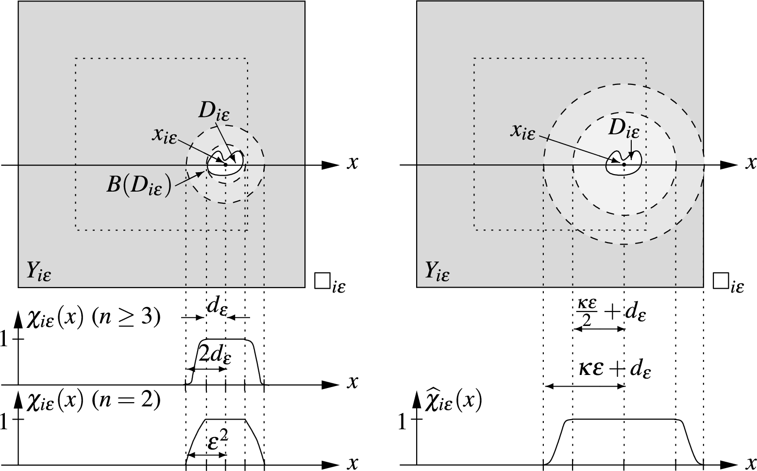
We define the operator $J_{ε}^{1'}$ being equal to $J_{ε}^{'}$ on $H_{ε}^{1}$ . Thus the only non-obvious definition is the one of $J_{ε}^{1}$ as we have to assure that $J_{ε}^{1} f ↾_{⋃_{i \in I_{ε}} D_{i ε}} = 0$ .

Fig. 3.

The two cut-off functions $χ_{i ε}$ and ${\hat{χ}}_{i ε}$ with decay on the scale $d_{ε}$ and ε, respectively. On the left, there is the cut-off function $χ_{i ε}$ , which is 1 inside the small ball $B (D_{i ε})$ (light gray) with radius $d_{ε}$ , and 0 outside the larger ball around $x_{i ε}$ with radius $2 d_{ε}$ ( $n ⩾ 3$ ) resp. $ε^{2}$ ( $n = 2$ ). On the right, there is the cut-off function ${\hat{χ}}_{i ε}$ , which is 1 inside the light gray ball of radius $κ ε / 2 + d_{ε}$ , and 0 on the dark gray area outside the larger ball of radius $κ ε + d_{ε}$ . Both cut-off functions have support in $□_{i ε}$ .

We define $\begin{matrix} J_{ε}^{1} f : = f - \sum_{i \in I_{ε}} P_{i ε} f - \sum_{i \in I_{ε}} Q_{i ε} f \end{matrix}$ with $\begin{matrix} (P_{i ε} f) (x) : = (f (x) - f_{i ε}) χ_{i ε} (x) and (Q_{ε} f) (x) : = f_{i ε} H_{i ε} (x) {\hat{χ}}_{i ε} (x) . \end{matrix}$ Here (see also Fig. 3)

$f_{i ε} : = {⟨ f ⟩}_{□_{i ε}}$ ,

$x_{i ε}$ denotes the center of the smallest ball $B (D_{i ε})$ containing the set $D_{i ε}$ (recall that this ball has radius $d_{ε}$ ),

for $n ⩾ 3$ : $\begin{matrix} χ_{i ε} (x) = χ (\frac{| x - x_{i ε} |}{d_{ε}}), \end{matrix}$ where $χ \in C^{\infty} (R)$ is a smooth cut-off function such that $| χ (t) | ⩽ 1$ and $\begin{matrix} χ (t) = 1 as t < 1 and χ (t) = 0 as t > 2, \end{matrix}$

for $n = 2$ : $\begin{matrix} χ_{i ε} (x) = \{\begin{matrix} 1 & as | x - x_{i ε} | ⩽ d_{ε}, \\ \frac{ln | x - x_{i ε} | - 2 ln ε}{ln d_{ε} - 2 ln ε} & as | x - x_{i ε} | \in (d_{ε}, ε^{2}), \\ 0 & as | x - x_{i ε} | ⩾ ε^{2}, \end{matrix} \end{matrix}$

${\hat{χ}}_{i ε} (x) : = χ (\frac{(2 / κ) \cdot (| x - x_{i ε} | - d_{ε})}{ε})$ ,

for $n ⩾ 3$ : $H_{i ε}$ is the solution to the problem $\begin{array}{l} \{\begin{matrix} Δ H_{i ε} (x) = 0, & x \in R^{n} ∖ \overline{D_{i ε}}, \\ H_{i ε} (x) = 1, & x \in \partial D_{i ε}, \\ H_{i ε} (x) \to 0, & | x | \to \infty, \end{matrix} \end{array}$

for $n = 2$ : $H_{i ε}$ is the solution to the problem $\begin{array}{l} \{\begin{matrix} Δ H_{i ε} (x) = 0, & x \in B_{1} (x_{i ε}) ∖ \overline{D_{i ε}}, \\ H_{i ε} (x) = 1, & x \in \partial D_{i ε}, \\ H_{i ε} (x) = 0, & x \in \partial B_{1} (x_{i ε}), \end{matrix} \\ B_{1} (x_{i ε}) is the unit ball centered at x_{i ε}, \end{array}$ extended by 0 to $R^{n} ∖ \overline{B_{1} (x_{i ε})}$ .

Note, that the function

H_{i ε}

is defined on

R^{n} ∖ D_{i ε}

(resp.

B_{1} (x_{i ε}) ∖ D_{i ε}

n = 2

). We extend it onto

D_{i ε}

by 1 (and onto

R^{n} ∖ B_{1} (x_{i ε})

by 0 if

n = 2

), keeping the same notation

H_{i ε}

. Note also that

‖ \nabla H_{i ε} ‖_{L_{2} (R^{n})}^{2} = cap (D_{i ε})

by the definition of capacity in (8) and (11).

We set $Y_{i ε} : = □_{i ε} ∖ \overline{D_{i ε}}$ . It is easy to see that $\begin{array}{l} P_{i ε} f ↾_{D_{i ε}} = f ↾_{D_{i ε}} - f_{i ε}, Q_{i ε} f ↾_{D_{i ε}} = f_{i ε}, supp (P_{i ε} f) \subset □_{i ε}, supp (Q_{i ε} f) \subset □_{i ε} \end{array}$ (the inclusions are valid for $d_{ε} ⩽ κ ε$ , which holds true for small enough ε in view of (5)). Consequently $J_{ε}^{1} f \in H_{0}^{1} (Ω_{ε})$ .

Now, we are in position to start the proof of ( C 1 a )–( C 5 ).

At first, we note that conditions ( C 1 b ), ( C 2 ), ( C 4 b ) hold with $δ_{ε} = 0$ , following from the definitions of the operators $J_{ε}$ , $J_{ε}^{'}$ and $J_{ε}^{1'}$ . Also, obviously, for each $f \in L_{2} (Ω)$ and $u \in L_{2} (Ω_{ε})$ we have $\begin{matrix} ‖ J_{ε} f ‖_{L_{2} (Ω_{ε})} ⩽ ‖ f ‖_{L_{2} (Ω)}, {‖ J_{ε}^{'} u ‖}_{L_{2} (Ω)} = ‖ u ‖_{L_{2} (Ω_{ε})}, \end{matrix}$ and therefore conditions ( C 3 a )–( C 3 b ) are valid as well with $δ_{ε} = 0$ . Thus, it remains to check the non-trivial conditions ( C 1 a ), ( C 4 a ) and ( C 5 ).

The following Friedrichs- and Poincare-type inequalities will be frequently used further.

Lemma 4.1.

One has $\begin{array}{l} (26) & \forall v \in H_{0}^{1} (□_{i ε}) : ‖ v ‖_{L_{2} (□_{i ε})}^{2} ⩽ C ε^{2} ‖ \nabla v ‖_{L_{2} (□_{i ε})}^{2}, \\ (27) & \forall v \in H^{1} (□_{i ε}) : ‖ v - {⟨ v ⟩}_{□_{i ε}} ‖_{L_{2} (□_{i ε})}^{2} ⩽ C ε^{2} ‖ \nabla v ‖_{L_{2} (□_{i ε})}^{2} . \end{array}$

Proof.

By the min–max principle $\begin{array}{l} Λ_{ε}^{D} = min {\frac{‖ \nabla u ‖_{L_{2} (□_{i ε})}^{2}}{‖ u ‖_{L_{2} (□_{i ε})}^{2}} : u \in H_{0}^{1} (□_{i ε}) ∖ {0}}, \\ Λ_{ε}^{N} = min {\frac{‖ \nabla u ‖_{L_{2} (□_{i ε})}^{2}}{‖ u ‖_{L_{2} (□_{i ε})}^{2}} : u \in H^{1} (□_{i ε}) ∖ {0}, \int_{□_{i ε}} u (x) d x = 0}, \end{array}$ where $Λ_{ε}^{D}$ (respectively, $Λ_{ε}^{N}$ ) is the first (respectively, the second) eigenvalue of the Dirichlet (respectively, the Neumann) Laplacian on $□_{i ε}$ . Straightforward calculations gives $\begin{array}{l} λ_{ε}^{D} = n {(\frac{π}{ε})}^{2}, λ_{ε}^{N} = {(\frac{π}{ε})}^{2}, \end{array}$ hence we easily get the required inequalities (26)–(27). □

4.1. Proof of ( C 1 a )

Let $f \in L_{2} (Ω)$ . We have $\begin{array}{l} (28) & ‖ J_{ε} f - J_{ε}^{1} f ‖_{H_{ε}}^{2} ⩽ 2 \sum_{i \in I_{ε}} (‖ P_{i ε} f ‖_{L_{2} (□_{i ε})}^{2} + ‖ Q_{i ε} f ‖_{L_{2} (□_{i ε})}^{2}) . \end{array}$

Using (27) and taking into account that $| χ_{i ε} (x) | ⩽ 1$ , we obtain: $\begin{array}{l} (29) & \sum_{i \in I_{ε}} ‖ P_{i ε} f ‖_{L_{2} (□_{i ε})}^{2} ⩽ \sum_{i \in I_{ε}} ‖ f - f_{i ε} ‖_{L_{2} (□_{i ε})}^{2} ⩽ C ε^{2} \sum_{i \in I_{ε}} ‖ \nabla f ‖_{L_{2} (□_{i ε})}^{2} ⩽ C ε^{2} ‖ f ‖_{H^{1}}^{2} . \end{array}$

Using (26) and taking into account that $| {\hat{χ}}_{i ε} | ⩽ 1$ , $| {\hat{χ}}_{i ε}^{'} | ⩽ C κ^{- 1} ε^{- 1}$ and ${\hat{χ}}_{i ε} ↾_{D_{i ε}} = H_{i ε} ↾_{D_{i ε}} = 1$ we obtain: $\begin{matrix} (30) & \begin{matrix} \sum_{i \in I_{ε}} ‖ Q_{i ε} f ‖_{L_{2} (□_{i ε})}^{2} & ⩽ \sum_{i \in I_{ε}} | f_{i ε} |^{2} ‖ {\hat{χ}}_{i ε} H_{i ε} ‖_{L_{2} (□_{i ε})}^{2} ⩽ C ε^{2} \sum_{i \in I_{ε}} | f_{i ε} |^{2} ‖ \nabla ({\hat{χ}}_{i ε} H_{i ε}) ‖_{L_{2} (Y_{i ε})}^{2} \\ ⩽ C_{1} ε^{2} \sum_{i \in I_{ε}} | f_{i ε} |^{2} (‖ \nabla H_{i ε} ‖_{L_{2} (Y_{i ε})}^{2} + κ^{- 2} ε^{- 2} ‖ H_{i ε} ‖_{L_{2} (supp (\nabla {\hat{χ}}_{i ε}))}^{2}) . \end{matrix} \end{matrix}$ From (7) and the definition of $H_{i ε}$ we obtain the estimate $\begin{array}{l} (31) & ‖ \nabla H_{i ε} ‖_{L_{2} (Y_{i ε})}^{2} ⩽ ‖ \nabla H_{i ε} ‖_{L_{2} (R^{n})}^{2} = cap (D_{i ε}) ⩽ C ε^{n} . \end{array}$ Using Lemma 2.1, we obtain $\begin{matrix} | H_{i ε} (x) | ⩽ C τ_{n} (d_{ε}) / τ_{n} (ε), where τ_{n} (r) : = \{\begin{matrix} r^{n - 2}, & n ⩾ 3, \\ | ln r |^{- 1}, & n = 2 \end{matrix} \end{matrix}$ for $x \in supp (\nabla {\hat{χ}}_{i ε}) \subset {x \in R^{n} : d_{ε} + κ ε / 2 ⩽ | x - x_{i ε} | ⩽ d_{ε} + κ ε}$ . Hence, taking into account that $τ_{n} (d_{ε}) ⩽ C ε^{n}$ (see (5)), we deduce the asymptotics $\begin{array}{l} (32) & ‖ H_{i ε} ‖_{L_{2} (supp (\nabla χ_{i ε}))}^{2} = o (ε^{n + 2}) . \end{array}$ Finally, applying the Cauchy–Schwarz inequality, one gets $\begin{array}{l} (33) & | f_{i ε} |^{2} ⩽ ε^{- n} ‖ f ‖_{L_{2} (□_{i ε})}^{2} . \end{array}$ Combining (30)–(33) we arrive at $\begin{array}{l} (34) & \sum_{i \in I_{ε}} ‖ Q_{i ε} f ‖_{L_{2} (□_{i ε})}^{2} ⩽ C_{κ} ε^{2} ‖ f ‖_{H}^{2} . \end{array}$ Here and in what follows by $C_{κ}$ we denote a generic constant depending on κ and n.

From (28), (29), (34) we obtain $\begin{array}{l} {‖ J_{ε} f - J_{ε}^{1} f ‖}_{H_{ε}} ⩽ C_{κ} ε ‖ f ‖_{H^{1}} ⩽ δ_{ε} ‖ f ‖_{H^{1}}, \end{array}$ where $δ_{ε}$ is defined in (17). Therefore, we have checked Condition ( C 1 a ).

4.2. Proof of ( C 4 a )

We need the following lemma, which was proven in [29, Lem. 4.9 and Rem. 4.2].

Lemma 4.2.
Let $D \subset R^{n}$ be a bounded convex domain, and let $D_{1}, D_{2} \subset D$ be measurable subsets with $| D_{2} | \neq 0$ . Then $\begin{matrix} ‖ v ‖_{L_{2} (D_{1})}^{2} ⩽ \frac{2 | D_{1} |}{| D_{2} |} ‖ v ‖_{L_{2} (D_{2})}^{2} + C \frac{{(diam (D))}^{n + 1} | D_{1} |^{1 / n}}{| D_{2} |} ‖ \nabla v ‖_{L_{2} (D)}^{2} \end{matrix}$ for all $v \in H^{1} (D)$ , where C depends only on the dimension n.

Let $f \in L_{2} (Ω)$ . Applying Lemma 4.2 with $v : = f$ and $D : = □_{i ε}$ , $D_{1} : = D_{i ε}$ , $D_{2} : = □_{i ε}$ we obtain $\begin{matrix} ‖ f - J_{ε}^{'} J_{ε} f ‖_{H}^{2} & = \sum_{i \in I_{ε}} ‖ f ‖_{L_{2} (D_{i ε})}^{2} ⩽ C \sum_{i \in I_{ε}} ({(\frac{d_{ε}}{ε})}^{n} ‖ f ‖_{L_{2} (□_{i ε})}^{2} + \frac{ε^{n + 1} d_{ε}}{ε^{n}} ‖ \nabla f ‖_{L_{2} (□_{i ε})}^{2}) \\ ⩽ C ({(\frac{d_{ε}}{ε})}^{n} + ε d_{ε}) ‖ f ‖_{H^{1}}^{2} . \end{matrix}$ It is straightforward to show, using (5) and the definition of $δ_{ε}$ in (17), that $\begin{matrix} {(\frac{d_{ε}}{ε})}^{n} + ε d_{ε} ⩽ C ε^{2} ⩽ C {(δ_{ε})}^{2} \end{matrix}$ and thus condition ( C 4 a ) is also valid.
4.3. Proof of the form estimate ( C 5 )

We will show that ( C 5 ) holds with $k = 2$ .

Recall that $H^{2}$ is a Hilbert space consisting of functions from $dom (A) = H^{2} (Ω) \cap H_{0}^{1} (Ω)$ with scalar product ${(f, g)}_{H^{2}} : = {(A f + f, A g + g)}_{H}$ .

Since $\partial Ω$ is $C^{2}$ -smooth, we can apply standard elliptic regularity theory (see, e.g., [18]): namely, the $H^{2}$ -norm is equivalent to the $H^{2} (Ω)$ -norm, i.e. there is $C_{Ω} > 0$ such that for each $f \in dom (A)$ we have $\begin{array}{l} (35) & ‖ f ‖_{H^{2} (Ω)} ⩽ C_{Ω} ‖ f ‖_{H^{2}} \end{array}$ (the fulfilment of (35) for noncompact $\partial Ω$ is due to the uniform regularity of Ω).

Note, that this is the only estimate in our proof in which the constant depends on the domain Ω. This results in Ω-dependence of the constant standing in the definition of $δ_{ε}$ .

Let $f \in dom (A)$ , $u \in H_{0}^{1} (Ω_{ε})$ . One has: $\begin{array}{l} | a_{ε} [u, J_{ε}^{1} f] - a [J_{ε}^{1'} u, f] | \\ ⩽ | \sum_{i \in I_{ε}} {(\nabla u, \nabla P_{i ε} f)}_{L_{2} (Y_{i ε})} | + | \sum_{i \in I_{ε}} {(\nabla u, \nabla Q_{i ε} f)}_{L_{2} (Y_{i ε})} + q {(u, f)}_{L_{2} (Ω_{ε})} | = : J_{ε, 1} + J_{ε, 2} . \end{array}$

4.3.1. Estimates for $J_{ε, 1}$

One has, taking into account that $| χ_{i ε} (x) | ⩽ 1$ : $\begin{matrix} (36) & \begin{matrix} J_{ε, 1} & ⩽ | \sum_{i \in I_{ε}} {(\nabla u, χ_{i ε} \nabla f)}_{L_{2} (supp (χ_{i ε}))} | + | \sum_{i \in I_{ε}} {(\nabla u, (f - f_{i ε}) \nabla χ_{i ε})}_{L_{2} (supp (χ_{i ε}))} | \\ ⩽ ‖ \nabla u ‖_{L_{2} (Ω_{ε})} ({(\sum_{i \in I_{ε}} ‖ \nabla f ‖_{L_{2} (supp (χ_{i ε}))}^{2})}^{\frac{1}{2}} + {(\sum_{i \in I_{ε}} ‖ (f - f_{i ε}) \nabla χ_{i ε} ‖_{L_{2} (Y_{i ε})}^{2})}^{\frac{1}{2}}) . \end{matrix} \end{matrix}$

Applying Lemma 4.2 with $v : = \partial_{j} f$ , $D : = □_{i ε}$ , $D_{1} : = supp (χ_{i ε})$ and $D_{2} : = □_{i ε}$ , and taking into account (5) and (35) we obtain the estimates: $\begin{matrix} (37) & \begin{array}{l} n ⩾ 2 : \sum_{i \in I_{ε}} ‖ \nabla f ‖_{L_{2} (supp (χ_{i ε}))}^{2} ⩽ C ({(\frac{d_{ε}}{ε})}^{n} + ε \cdot d_{ε}) ‖ f ‖_{H^{2} (Ω)}^{2} ⩽ C ε^{2} ‖ f ‖_{H^{2}}^{2}, \\ n = 2 : \sum_{i \in I_{ε}} ‖ \nabla f ‖_{L_{2} (supp (χ_{i ε}))}^{2} ⩽ C ({(\frac{ε^{2}}{ε})}^{2} + ε \cdot ε^{2}) ‖ f ‖_{H^{2} (Ω)}^{2} ⩽ C ε^{2} ‖ f ‖_{H^{2}}^{2} . \end{array} \end{matrix}$

Now, we estimate the second term in (36). One has the following Hölder-type inequality: $\begin{array}{l} (38) & \forall p, q \in [2, \infty], \frac{1}{p} + \frac{1}{q} = \frac{1}{2} : {‖ (f - f_{i ε}) \nabla χ_{i ε} ‖}_{L_{2} (Y_{i ε})} ⩽ ‖ f - f_{i ε} ‖_{L_{p} (Y_{i ε})} ‖ \nabla χ_{i ε} ‖_{L_{q} (Y_{i ε})} \end{array}$ (for $p = \infty$ we use a convention $p^{- 1} = 0$ ). Indeed, the classical Hölder inequality states that $‖ F G ‖_{L_{1} (Y_{i ε})} ⩽ ‖ F ‖_{L_{p} (Y_{i ε})} ‖ G ‖_{L_{q} (Y_{i ε})}$ provided $p, q \in [1, \infty]$ , $p^{- 1} + q^{- 1} = 1$ . Setting $p : = p / 2$ , $q : = q / 2$ , $F : = | f - f_{i ε} |^{2}$ , $G : = | \nabla χ_{i ε} |^{2}$ we easily arrive at (38).

One needs the following re-scaled Sobolev inequality.

Lemma 4.3.
For each $f \in H^{2} (□_{i ε})$ $\begin{array}{l} (39) & ‖ f - f_{i ε} ‖_{L_{p} (□_{i ε})} ⩽ C_{p} ε^{n / p + (2 - n) / 2} ‖ f ‖_{H^{2} (□_{i ε})} \end{array}$ provided p satisfies $\begin{array}{l} (40) & 2 ⩽ p ⩽ \frac{2 n}{n - 4} as n ⩾ 5, 2 ⩽ p < \infty as n = 4, p = \infty as n = 2, 3 . \end{array}$ The constant $C_{p}$ depends only on p.
Proof.
Recall that $□ = {(- 1 / 2, 1 / 2)}^{n}$ . Since $H^{2} (□) ↪ L_{p} (□)$ provided (40) holds (see, e.g., [1, Theorem 5.4]) one has for each $g \in H^{2} (□)$ : $\begin{array}{l} (41) & ‖ g ‖_{L_{p} (□)} ⩽ C_{p} ‖ g ‖_{H^{2} (□)} . \end{array}$ Now, making the change of variables $□ ∋ x = y ε^{- 1} - i$ with $y \in □_{i ε}$ in (41), we infer from (41): for each $g \in H^{2} (□_{i ε})$ $\begin{array}{l} (42) & ε^{- n / p} ‖ g ‖_{L_{p} (□)} ⩽ C_{p} {(ε^{- n} ‖ g ‖_{L_{2} (□_{i ε})}^{2} + ε^{2 - n} ‖ \nabla g ‖_{L_{2} (□_{i ε})}^{2} + ε^{4 - n} \sum_{k, l = 1}^{n} ‖ \partial_{k l}^{2} g ‖_{L_{2} (□_{i ε})}^{2})}^{1 / 2} . \end{array}$ Finally, we set $g : = f - f_{i ε}$ . Then, due to (27), the estimate (42) becomes $\begin{array}{l} ‖ f - f_{i ε} ‖_{L_{p} (□)} & ⩽ C_{p} ε^{n / p} {(ε^{2 - n} ‖ \nabla f ‖_{L_{2} (□_{i ε})}^{2} + ε^{4 - n} \sum_{k, l = 1}^{n} ‖ \partial_{k l}^{2} f ‖_{L_{2} (□_{i ε})}^{2})}^{1 / 2} \\ ⩽ C_{p} ε^{n / p + (2 - n) / 2} ‖ f ‖_{H^{2} (□_{i ε})} . \end{array}$ □

We also need the estimate for $χ_{i ε}$ , which is proved via a straightforward calculations.
Lemma 4.4.
One has $\begin{matrix} (43) & \begin{array}{l} ‖ \nabla χ_{i ε} ‖_{L_{q} (Y_{i ε})} ⩽ C {(d_{ε})}^{n / q - 1}, n ⩾ 3, q \in [2, \infty], \\ ‖ \nabla χ_{i ε} ‖_{L_{2} (Y_{i ε})} ⩽ C | ln d_{ε} |^{- 1 / 2}, n = 2 . \end{array} \end{matrix}$

Now, we choose the largest p for which (40) holds: $\begin{array}{l} p : = \frac{2 n}{n - 4} as n ⩾ 5, \\ (44) & p : = 4 β^{- 1} with β \in (0, 2) as n = 4, \\ p = \infty as n = 2, 3 . \end{array}$ As before $\begin{array}{l} (45) & q = {(\frac{1}{2} - \frac{1}{p})}^{- 1} . \end{array}$

Plugging the estimates (39) and (43) into (38) and taking into account (5), (44)–(45) we arrive easily at $\begin{array}{l} n ⩾ 5 : {(\sum_{i \in I_{ε}} ‖ (f - f_{i ε}) \nabla χ_{i ε} ‖_{L_{2} (Y_{i ε})}^{2})}^{1 / 2} ⩽ C \cdot \frac{d_{ε}}{ε} ‖ f ‖_{H^{2} (Ω)}, \\ n = 4 : {(\sum_{i \in I_{ε}} ‖ (f - f_{i ε}) \nabla χ_{i ε} ‖_{L_{2} (Y_{i ε})}^{2})}^{1 / 2} ⩽ C_{β} \cdot {(\frac{d_{ε}}{ε})}^{1 - β} ‖ f ‖_{H^{2} (Ω)} ⩽ C_{β} ε^{1 - β} ‖ f ‖_{H^{2} (Ω)}, \\ (46) \\ n = 3 : {(\sum_{i \in I_{ε}} ‖ (f - f_{i ε}) \nabla χ_{i ε} ‖_{L_{2} (Y_{i ε})}^{2})}^{1 / 2} ⩽ C \cdot {(\frac{d_{ε}}{ε})}^{1 / 2} ‖ f ‖_{H^{2} (Ω)} ⩽ C ε ‖ f ‖_{H^{2} (Ω)}, \\ n = 2 : {(\sum_{i \in I_{ε}} ‖ (f - f_{i ε}) \nabla χ_{i ε} ‖_{L_{2} (Y_{i ε})}^{2})}^{1 / 2} ⩽ C | ln d_{ε} |^{- \frac{1}{2}} ‖ f ‖_{H^{2} (Ω)} ⩽ C ε ‖ f ‖_{H^{2} (Ω)} . \end{array}$

Combining (37) and (46) and taking into account (35) and the definition of $δ_{ε}$ , we get the estimate $\begin{array}{l} (47) & J_{ε, 1} ⩽ δ_{ε} ‖ u ‖_{H^{1}} ‖ f ‖_{H^{2}} . \end{array}$
4.3.2. Estimates for $J_{ε, 2}$

One has $\begin{array}{l} (48) & J_{ε, 2} = | \sum_{i \in I_{ε}} f_{i ε} {(\nabla u, \nabla (H_{i ε} {\hat{χ}}_{i ε}))}_{L_{2} (Y_{i ε})} + q {(u, f)}_{L_{2} (Ω_{ε})} | . \end{array}$

Besides (8) (or (11) for $n = 2$ ) there is another equivalent characterization of the capacity.

Lemma 4.5.
Let $D \subset R^{n}$ , and let H be the solution of either ( 9 ) if $n ⩾ 3$ or ( 12 ) if $n = 2$ . Then $\begin{array}{l} (49) & cap (D) = - \int_{\partial D} \frac{\partial H}{\partial ν} d s, \end{array}$ where ν is the outward-pointing unit normal to $\partial D$ , $d s$ is the area measure on $\partial D$ .
Proof.
For $n = 2$ the result follows from $\begin{matrix} \int_{\partial D} \frac{\partial H}{\partial ν} d s = \int_{\partial D} \frac{\partial H}{\partial ν} H d s = - \int_{B_{1} ∖ \overline{D}} | \nabla H |^{2} d x . \end{matrix}$ Here the first equality is due to $H ↾_{\partial D} = 1$ , while the second one is the Green formula, in which the surface integral over $\partial B_{1}$ vanishes since $H ↾_{\partial B_{1}} = 0$ , and the second volume integral vanishes since $Δ H = 0$ .

For $n ⩾ 3$ we proceed as follows. Let $B_{R}$ be the ball of radius $R > 1$ being concentric with the smallest ball containing D. One has: $\begin{array}{l} (50) & \int_{\partial D} \frac{\partial H}{\partial ν} d s = \int_{\partial D} \frac{\partial H}{\partial ν} H d s = - \int_{B_{R} ∖ \overline{D}} | \nabla H |^{2} d x - \int_{\partial B_{R}} \frac{\partial H}{\partial ν} H d s \end{array}$ (in the last integral ν is the inward-pointing unit normal to $\partial B_{R}$ ). Lemma 2.1 implies the estimate $\begin{array}{l} (51) & | \int_{\partial B_{R}} \frac{\partial H}{\partial ν} H d s | ⩽ \frac{C}{R^{n - 2}} . \end{array}$ Passing to the limit $R \to \infty$ in (50) and taking into account (8) and (51) we arrive at the required equality (49). The lemma is proved. □

Denote $u_{i ε} : = {⟨ J_{ε}^{'} u ⟩}_{□_{i ε}}$ . Integrating by parts and using (49) we get $\begin{matrix} (52) & \begin{matrix} [b] & \sum_{i \in I_{ε}} f_{i ε} {(\nabla u, \nabla (H_{i ε} {\hat{χ}}_{i ε}))}_{L_{2} (Y_{i ε})} \\ = - \sum_{i \in I_{ε}} f_{i ε} {(u, Δ (H_{i ε} {\hat{χ}}_{i ε}))}_{L_{2} (Y_{i ε})} = - \sum_{i \in I_{ε}} f_{i ε} u_{i ε} {(1, Δ (H_{i ε} {\hat{χ}}_{i ε}))}_{L_{2} (Y_{i ε})} + ζ_{ε} \\ = \sum_{i \in I_{ε}} f_{i ε} u_{i ε} \int_{\partial D_{i ε}} \frac{\partial H_{i ε}}{\partial ν} d s + ζ_{ε} = - \sum_{i \in I_{ε}} f_{i ε} u_{i ε} cap (D_{ε}) + ζ_{ε}, \end{matrix} \end{matrix}$ where $ζ_{ε} = \sum_{i \in I_{ε}} f_{i ε} {(u_{i ε} - u, Δ (H_{i ε} {\hat{χ}}_{i ε}))}_{L_{2} (Y_{i ε})}$ . Here we have used the facts that ${\hat{χ}}_{i ε}$ vanishes on ${x \in Y_{i ε} : | x - x_{i ε} | ⩾ d_{ε} + ε κ}$ with all its derivatives, $u ↾_{\partial D_{i ε}} = 0$ , and ${\hat{χ}}_{i ε} (x) = 1$ in a neighbourhood of $D_{i ε}$ .

The remainder term $ζ_{ε}$ is small; namely the following estimate holds:
Lemma 4.6.
One has: $\begin{array}{l} (53) & | ζ_{ε} | ⩽ C_{κ} \cdot \{\begin{matrix} ε ‖ \nabla u ‖_{L_{2} (Ω_{ε})} ‖ f ‖_{L_{2} (Ω)}, & n ⩾ 3, \\ ε | ln ε | ‖ \nabla u ‖_{L_{2} (Ω_{ε})} ‖ f ‖_{L_{2} (Ω)}, & n = 2 . \end{matrix} \end{array}$
Proof.
At first we consider the case $n ⩾ 3$ . Since $Δ H_{i ε} = 0$ we have $\begin{array}{l} Δ (H_{i ε} {\hat{χ}}_{i ε}) = 2 \nabla H_{i ε} \cdot \nabla {\hat{χ}}_{i ε} + H_{i ε} Δ {\hat{χ}}_{i ε}, \\ supp (Δ (H_{i ε} {\hat{χ}}_{i ε})) \subset {x \in Y_{i ε} : d_{ε} + κ ε / 2 ⩽ | x - x_{i ε} | ⩽ d_{ε} + κ ε}, \end{array}$ hence, due to Lemma 2.1, (5) and $| \nabla {\hat{χ}}_{i ε} (x) | ⩽ C κ^{- 1} ε^{- 1}$ , $| Δ {\hat{χ}}_{i ε} (x) | ⩽ C κ^{- 2} ε^{- 2}$ , we get $\begin{array}{l} (54) & | (Δ (H_{i ε} {\hat{χ}}_{i ε})) (x) | ⩽ C (\frac{{(d_{ε})}^{n - 2}}{ε^{n - 1}} \cdot \frac{1}{κ ε} + \frac{{(d_{ε})}^{n - 2}}{ε^{n - 2}} \cdot \frac{1}{κ^{2} ε^{2}}) ⩽ C_{κ} . \end{array}$ Then, using the Cauchy–Schwarz inequality, (27) and (54), we obtain $\begin{array}{l} | ζ_{ε} | ⩽ C_{κ} {(\sum_{i \in I_{ε}} {‖ J_{ε}^{'} u - u_{i ε} ‖}_{L_{2} (□_{i ε})})}^{1 / 2} {(\sum_{i \in I_{ε}} | f_{i ε} |^{2} ε^{n})}^{1 / 2} ⩽ C_{κ} ε ‖ \nabla u ‖_{L_{2} (Ω_{ε})} ‖ f ‖_{L_{2} (Ω)} . \end{array}$

In the case $n = 2$ Lemma 2.1 gives $\begin{array}{l} | (Δ (H_{i ε} {\hat{χ}}_{i ε})) (x) | ⩽ C_{κ} | ln ε |, \end{array}$ and, via the same arguments as in the case $n ⩾ 3$ , we obtain $\begin{array}{l} | ζ_{ε} | ⩽ C_{κ} ε | ln ε | ‖ \nabla u ‖_{L_{2} (Ω_{ε})} ‖ f ‖_{L_{2} (Ω)} . \end{array}$ The lemma is proved. □

We need also the estimate for $H_{0}^{1} (Ω)$ -functions in a neighbourhood of $\partial Ω$ .
Lemma 4.7.
Let $T_{ε} = Ω_{ε} ∖ \overline{⋃_{i \in I_{ε}} Y_{i ε}}$ . One has for each $f \in H_{0}^{1} (Ω)$ : $\begin{array}{l} (55) & ‖ f ‖_{L_{2} (T_{ε})} ⩽ C ε ‖ \nabla f ‖_{L_{2} (Ω)} . \end{array}$
Proof.
We denote $\begin{matrix} {\hat{Ω}}_{ε} = {y \in R^{n} : y = x + t ν (x), x \in \partial Ω, t \in [0, \sqrt{n} ε)} \end{matrix}$ (recall that $ν : \partial Ω \to S^{n - 1}$ is a unit inward-pointing normal vector field on $\partial Ω$ ). Note, that $\sqrt{n}$ is the length of the diagonal of the cube □. Taking this into account one can easily deduce from the definition of the set $I_{ε}$ that $T_{ε} \subset {\hat{Ω}}_{ε}$ .

Let $Δ_{{\hat{Ω}}_{ε}}$ be the Laplace operator on ${\hat{Ω}}_{ε}$ subject to the Dirichlet conditions on $\partial Ω$ and the Neumann conditions on $\partial {\hat{Ω}}_{ε} ∖ \partial Ω$ . One has the following asymptotic equality (see [26]): $\begin{matrix} inf σ (- Δ_{{\hat{Ω}}_{ε}}) = {(\frac{π}{2 \sqrt{n} ε})}^{2} + \frac{C_{Ω}}{ε} + O (1), \end{matrix}$ where the constant $C_{Ω}$ depends on the principal curvatures of $\partial Ω$ . Note, that the result of [26] is obtained under the assumption that the map (4) is injective on $\partial Ω \times [0, \sqrt{n} ε]$ , that indeed holds true provided ε is small enough, namely $ε < θ_{Ω} / \sqrt{n}$ .

Hence, using the minimax principle, we get the inequality $\begin{array}{l} (56) & ‖ f ‖_{L_{2} ({\hat{Ω}}_{ε})}^{2} ⩽ C ε^{2} ‖ \nabla f ‖_{L_{2} ({\hat{Ω}}_{ε})}^{2}, \end{array}$ which holds for each $f \in H^{1} ({\hat{Ω}}_{ε})$ with $f ↾_{\partial Ω} = 0$ . Obviously, (55) follows from (56). □

Using (27), (52), (55) we obtain from (48): $\begin{matrix} J_{ε, 2} & ⩽ | ζ_{ε} | + | \sum_{i \in I_{ε}} f_{i ε} u_{i ε} cap (D_{ε}) - q \sum_{i \in I_{ε}} {(f, u)}_{L_{2} (Y_{i ε})} | + q | {(f, u)}_{L_{2} (T_{ε})} | \\ ⩽ | ζ_{ε} | + | (cap (D_{ε}) ε^{- n} - q) \sum_{i \in I_{ε}} ε^{n} f_{i ε} u_{i ε} | + q | \sum_{i \in I_{ε}} {(f_{i ε} - f, u)}_{L_{2} (Y_{i ε})} | + q | {(f, u)}_{L_{2} (T_{ε})} | \\ ⩽ | ζ_{ε} | + | cap (D_{ε}) ε^{- n} - q | ‖ f ‖_{L_{2} (Ω_{ε})} ‖ u ‖_{L_{2} (Ω_{ε})} + q {(\sum_{i \in I_{ε}} ‖ f - f_{i ε} ‖_{L_{2} (□_{i ε})})}^{1 / 2} ‖ u ‖_{L_{2} (Ω_{ε})} \\ + q ‖ f ‖_{L_{2} (T_{ε})} ‖ u ‖_{L_{2} (T_{ε})} \\ ⩽ | ζ_{ε} | + | cap (D_{ε}) ε^{- n} - q | ‖ f ‖_{L_{2} (Ω_{ε})} ‖ u ‖_{L_{2} (Ω_{ε})} + C ε ‖ \nabla f ‖_{L_{2} (Ω)} ‖ u ‖_{L_{2} (Ω_{ε})} \\ + q ‖ f ‖_{L_{2} (T_{ε})} ‖ u ‖_{L_{2} (T_{ε})}, \end{matrix}$ hence, taking into account (53), we get $\begin{array}{l} (57) & J_{ε, 2} ⩽ δ_{ε} ‖ u ‖_{H^{1}} ‖ f ‖_{H^{1}} . \end{array}$

Combining estimates (47) and (57) we obtain ( C 5 ) with $k = 2$ .

Thus, we have checked the fulfilment of conditions ( C 1 a )–( C 5 ), hence we immediately get Theorems 2.3–2.6. Remark 4.8.
It is evident from the proof that the assumptions on $\partial Ω$ can be weakened. We use them twice: to guarantee the fulfilment of (35) (elliptic regularity) and to prove estimate (56), where we utilize the result from [26]. It is well-known, that the elliptic regularity is still valid under less restrictive assumptions, for example, if $\partial Ω$ is compact and belongs to $C^{1, 1}$ class or Ω is a convex domain with Lipschitz boundary (see, e.g., [21, Theorems 2.2.2.3 and 3.2.1.2]). Apparently, inequality (56) can be proved for Lipschitz domains under additional restrictions on principal curvatures.

4.4. Proof of Theorem 2.7

We will use the results of [22]. Let $H_{ε}$ and $H$ be separable Hilbert spaces, and $B_{ε} : H_{ε} \to H_{ε}$ , $B : H \to H$ be linear compact self-adjoint positive operators. We denote by ${μ_{k, ε}}_{k \in N}$ and ${μ_{k}}_{k \in N}$ the eigenvalues of the operators $B_{ε}$ and B, respectively, being renumbered in the descending order and with account of their multiplicity.

Theorem 4.9 ([22]).

Assume that the following conditions $A_{1}$ – $A_{4}$ hold:

The linear bounded operator $J_{ε} : H \to H_{ε}$ exists such that for each $f \in H$ $\begin{array}{l} ‖ J_{ε} f ‖_{H_{ε}} \to ‖ f ‖_{H} as ε \to 0 . \end{array}$

The norms $‖ B_{ε} ‖_{L (H_{ε})}$ are bounded uniformly in ε.

For any $f \in H$ : $‖ B_{ε} J_{ε} f - J_{ε} B f ‖_{H_{ε}} \to 0$ as $ε \to 0$ .

For any family ${f_{ε} \in H_{ε}}_{ε}$ with ${sup}_{ε} ‖ f_{ε} ‖_{H_{ε}} < \infty$ there exist a sequence ${(ε_{m})}_{m}$ and $w \in H$ such that $‖ B_{ε_{m}} f_{ε_{m}} - J_{ε_{m}} w ‖_{H_{ε_{m}}} \to 0$ and $ε_{m} \to 0$ as $m \to \infty$ .

Then for any $k \in N$ we have $\begin{matrix} | μ_{k, ε} - μ_{k} | ⩽ C_{ε} sup_{f} ‖ B_{ε} J_{ε} f - J_{ε} B f ‖_{H_{ε}}, \end{matrix}$ where $| C_{ε} | ⩽ C$ , ${lim}_{ε \to 0} C_{ε} = 1$ , the supremum is taken over all $f \in H$ belonging to the eigenspace associated with $μ_{k}$ and satisfying $‖ f ‖_{H} = 1$ .

We apply this theorem with $B_{ε} = {(A_{ε} + I)}^{- 1}$ , $B = {(A + I)}^{- 1}$ . These operators are positive, self-adjoint and compact (recall that Ω is a bounded domain here), moreover $‖ B_{ε} ‖_{L (H_{ε})} ⩽ 1$ . Thus condition $A_{2}$ is fulfilled. We choose the operator $J_{ε}$ by (15); due to (16) condition $A_{1}$ is valid. By Theorem 2.3 condition $A_{3}$ holds as well. Finally, since $‖ B_{ε} ‖_{L (H_{ε})} ⩽ 1$ , the set ${‖ B_{ε} f_{ε} ‖_{H^{1} (Ω_{ε})}}_{ε}$ is also bounded. Then the sequence ${J_{ε}^{'} B_{ε} f_{ε}}_{ε}$ is bounded in $H^{1} (Ω)$ (recall that the operator $J_{ε}^{'}$ is defined in (18)), and by Rellich’s embedding theorem it is compact in $L_{2} (Ω)$ provided Ω is bounded. Thus there exist $w \in L_{2} (Ω)$ and a sequence ${(ε_{m})}_{m}$ such that $‖ J_{ε_{m}}^{'} B_{ε_{m}} f_{ε_{m}} - w ‖_{L_{2} (Ω)} \to 0$ and $ε_{m} \to 0$ as $m \to \infty$ , hence we immediately obtain Condition $A_{4}$ .

Combining Theorems 2.3 and 4.9 we arrive at the estimate $\begin{matrix} (58) & | μ_{k, ε} - μ_{k} | ⩽ 4 C_{ε} δ_{ε}, \end{matrix}$ where $| C_{ε} | ⩽ C$ , ${lim}_{ε \to 0} C_{ε} = 1$ and $δ_{ε}$ is given in (17). Since $μ_{k, ε} = {(λ_{k, ε} + 1)}^{- 1}$ , and $μ_{k} = {(λ_{k} + 1)}^{- 1}$ , (58) is equivalent to (20).

Finally, we observe that for each fixed $k \in N$ $\begin{array}{l} (59) & λ_{k, ε} ⩽ C_{k} \end{array}$ that follows from Theorem 3.12 and Remark 3.11 (otherwise, we will easily obtain a contradiction with Condition (ii) from this remark). (20), (59) imply (19). Theorem 2.7 is proved.

Footnotes

Acknowledgements

This research was carried on when the first author was a postdoctoral researcher in Karlsruhe Institute of Technology. He gratefully acknowledges financial support by the Deutsche Forschungsgemeinschaft (DFG) through CRC 1173 “Wave phenomena: analysis and numerics”.

References

R.A.

Adams, Sobolev Spaces, Pure and Applied Mathematics, Vol. 65, Academic Press, New York, 1975.

Anné and

Post, Wildly perturbed manifolds: Norm resolvent and spectral convergence, arXiv e-prints, arXiv:1802.01124 [math.SP], 2018.

Balzano, Random relaxed Dirichlet problems, Ann. Mat. Pura Appl. (4) 153 (1988), 133–174. doi:10.1007/BF01762390.

Behrndt,

Langer,

Lotoreichik and

Rohleder, Quasi boundary triples and semi-bounded self-adjoint extensions, Proc. Roy. Soc. Edinburgh Sect. A 147 (2017), 895–916. doi:10.1017/S0308210516000421.

A.G.

Belyaev, Asymptotics of solutions of boundary value problems in periodically perforated domains with small holes, J. Math. Sci. 75 (1995), 1715–1749. doi:10.1007/BF02368672.

M.S.

Birman and

T.A.

Suslina, Second order periodic differential operators. Threshold properties and homogenization, St. Petersburg Math. J. 15 (2004), 639–714. doi:10.1090/S1061-0022-04-00827-1.

M.S.

Birman and

T.A.

Suslina, Averaging of periodic differential operators taking a corrector into account. Approximation of solutions in the Sobolev class

H^{1} (R^{d})

, St. Petersburg Math. J. 18 (2007), 857–955. doi:10.1090/S1061-0022-07-00977-6.

Borisov,

Bunoiu and

Cardone, On a waveguide with frequently alternating boundary conditions: Homogenized Neumann condition, Ann. Henri Poincaré 11 (2010), 1591–1627. doi:10.1007/s00023-010-0065-0.

Borisov,

Cardone and

Durante, Homogenization and norm-resolvent convergence for elliptic operators in a strip perforated along a curve, Proc. Roy. Soc. Edinburgh Sect. A 146 (2016), 1115–1158. doi:10.1017/S0308210516000019.

10.

Borisov,

Cardone,

Faella and

Perugia, Uniform resolvent convergence for strip with fast oscillating boundary, J. Differential Equations 255 (2013), 4378–4402. doi:10.1016/j.jde.2013.08.005.

11.

Braides, Γ-Convergence for Beginners, Oxford Lecture Series in Mathematics and Its Applications, Vol. 22, Oxford University Press, Oxford, 2002.

12.

F.E.

Browder, Estimates and existence theorems for elliptic boundary value problems, Proc. Nat. Acad. Sci. U.S.A. 45 (1959), 365–372. doi:10.1073/pnas.45.3.365.

13.

Chavel, Eigenvalues in Riemannian Geometry, Academic Press, Orlando, FL, 1984.

14.

G.A.

Chechkin,

A.L.

Piatnitski and

A.S.

Shamaev, Homogenization. Methods and Applications, American Mathematical Society, Providence, RI, 2007.

15.

K.D.

Cherednichenko and

A.V.

Kiselev, Norm-resolvent convergence of one-dimensional high-contrast periodic problems to a Kronig–Penney dipole-type model, Comm. Math. Phys. 349 (2017), 441–480. doi:10.1007/s00220-016-2698-4.

16.

Cioranescu and

Murat, Un terme étrange venu d’ailleurs, in: Nonlinear Partial Differential Equations and Their Applications. Collège de France Seminar, Vol. II (Paris, 1979/1980), Res. Notes in Math., Vol. 60, Pitman, Boston, MA, 1982, pp. 98–138, 389–390.

17.

Dondl,

Cherednichenko and

Rösler, Norm-resolvent convergence in perforated domains, Asymptot. Anal., to appear, arXiv e-prints, arXiv:1706.05859 [math.AP], 2017.

18.

Gilbarg and

N.S.

Trudinger, Elliptic Partial Differential Equations of Second Order, Springer-Verlag, Berlin, 1977.

19.

Griso, Error estimate and unfolding for periodic homogenization, Asymptot. Anal. 40 (2004), 269–286.

20.

Griso, Interior error estimate for periodic homogenization, Anal. Appl. 4 (2006), 61–79. doi:10.1142/S021953050600070X.

21.

Grisvard, Elliptic Problems in Nonsmooth Domains, Monographs and Studies in Mathematics, Vol. 24, Pitman, Boston, MA, 1985.

22.

G.A.

Iosif’yan,

O.A.

Oleinik and

A.S.

Shamaev, On the limit behavior of the spectrum of a sequence of operators defined in different Hilbert spaces, Russ. Math. Surv. 44 (1989), 195–196. doi:10.1070/RM1989v044n03ABEH002116.

23.

Kac, Probabilistic methods in some problems of scattering theory, Rocky Mountain J. Math. 4 (1974), 511–537. doi:10.1216/RMJ-1974-4-3-511.

24.

Kato, Perturbation Theory for Linear Operators, Springer-Verlag, New York, 1966.

25.

E.Y.

Khruslov, The method of orthogonal projections and the Dirichlet boundary value problem in domains with a “fine-grained” boundary, Mat. Sb. (N. S.) 88(130) (1972), 38–60.

26.

Krejčiřík, Spectrum of the Laplacian in narrow tubular neighbourhoods of hypersurfaces with combined Dirichlet and Neumann boundary conditions, Math. Bohem. 139 (2014), 185–193.

27.

V.A.

Marchenko and

E.Y.

Khruslov, Boundary-value problems with fine-grained boundary, Mat. Sb. (N. S.) 65(107) (1964), 458–472.

28.

V.A.

Marchenko and

E.Y.

Khruslov, Boundary Value Problems in Domains with a Fine-Grained Boundary, Izdat. “Naukova Dumka”, Kiev, 1974, in Russian.

29.

V.A.

Marchenko and

E.Y.

Khruslov, Homogenization of Partial Differential Equations, Birkhäuser Boston, Inc., Boston, MA, 2006.

30.

Mugnolo,

Nittka and

Post, Norm convergence of sectorial operators on varying Hilbert spaces, Oper. Matrices 7 (2013), 955–995. doi:10.7153/oam-07-54.

31.

Ozawa, On an elaboration of M. Kac’s theorem concerning eigenvalues of the Laplacian in a region with randomly distributed small obstacles, Comm. Math. Phys. 91 (1983), 473–487. doi:10.1007/BF01206016.

32.

G.C.

Papanicolaou and

S.R.

Varadhan, Diffusion in regions with many small holes, in: Stochastic Differential Systems (Proc. IFIP-WG 7/1 Working Conf., Vilnius, 1978), Lecture Notes in Control and Information Sci., Vol. 25, Springer, Berlin, 1980, pp. 190–206.

33.

Post, Spectral convergence of quasi-one-dimensional spaces, Ann. Henri Poincaré 7 (2006), 933–973. doi:10.1007/s00023-006-0272-x.

34.

Post, Spectral Analysis on Graph-Like Spaces, Lecture Notes in Mathematics, Vol. 2039, Springer, Heidelberg, 2012.

35.

Rauch, The mathematical theory of crushed ice, in: Partial Differential Equations and Related Topics, Ford Foundation Sponsored Program at Tulane University, January to May, 1974, Lecture Notes in Math., Vol. 446, Springer, Berlin, 1975, pp. 370–379. doi:10.1007/BFb0070611.

36.

Rauch, Scattering by many tiny obstacles, in: Partial Differential Equations and Related Topics, Ford Foundation Sponsored Program at Tulane University, January to May, 1974, Lecture Notes in Math., Vol. 446, Springer, Berlin, 1975, pp. 380–389. doi:10.1007/BFb0070612.

37.

Rauch and

Taylor, Potential and scattering theory on wildly perturbed domains, J. Funct. Anal. 18 (1975), 27–59. doi:10.1016/0022-1236(75)90028-2.

38.

Simon, Functional Integration and Quantum Physics, Pure and Applied Mathematics, Vol. 86, Academic Press, New York, 1979.

39.

T.A.

Suslina, Homogenization of elliptic operators with periodic coefficients in dependence of the spectral parameter, St. Petersburg Math. J. 27 (2016), 651–708. doi:10.1090/spmj/1412.

40.

Taylor, Partial Differential Equations II. Qualitative Studies of Linear Equations, Springer, New York, 2011.

41.

G.M.

Vainikko, Regular convergence of operators and approximate solution of equations, J. Soviet Math. 15 (1981), 675–705. doi:10.1007/BF01377042.

42.

V.V.

Zhikov, On operator estimates in homogenization theory, Dokl. Akad. Nauk 403 (2005), 305–308, in Russian.

43.

V.V.

Zhikov, On the spectral method in homogenization theory, Proc. Steklov Inst. Math. 3(250) (2005), 85–94.

44.

V.V.

Zhikov and

S.E.

Pastukhova, On operator estimates for some problems in homogenization theory, Russ. J. Math. Phys. 12 (2005), 515–524.

45.

V.V.

Zhikov and

S.E.

Pastukhova, On operator estimates in homogenization theory, Russ. Math. Surv. 71 (2016), 417–511. doi:10.1070/RM9710.

Operator estimates for the crushed ice problem

Abstract

Keywords

1. Introduction

Definition 3.1 (See [33, App.] or [34, Ch. 4]).

4. Proof of the main results

4.2. Proof of ( C 4 a )

4.3.1. Estimates for J ε , 1

Theorem 4.9 ([22]).

Footnotes

Acknowledgements

References

4.3.1. Estimates for $J_{ε, 1}$