Spectral non-self-adjoint analysis of complex Dirac,Pauli and Schrödinger operators with constant magnetic fields of full rank

Abstract

We consider Dirac, Pauli and Schrödinger quantum Hamiltonians with constant magnetic fields of full rank in $L^{2} (R^{2 d})$ , $d ⩾ 1$ , perturbed by non-self-adjoint (matrix-valued) potentials. On the one hand, we show the existence of non-self-adjoint perturbations, generating near each point of the essential spectrum of the operators, infinitely many (complex) eigenvalues. On the other hand, we give asymptotic behaviours of the number of the (complex) eigenvalues. In particular, for compactly supported potentials, our results establish non-self-adjoint extensions of Raikov–Warzel [Rev. in Math. Physics 14 (2002), 1051–1072] and Melgaard–Rozenblum [Commun. PDE. 28 (2003), 697–736] results. So, we show how the (complex) eigenvalues converge to the points of the essential spectrum asymptotically, i.e., up to a multiplicative explicit constant, as $\begin{matrix} \frac{1}{d!} {(\frac{| ln r |}{ln | ln r |})}^{d}, r ↘ 0, \end{matrix}$ in small annulus of radius $r > 0$ around the points of the essential spectrum.

Keywords

Quantum magnetic Hamiltonians of full rank non-self-adjoint (matrix-valued) perturbations complex eigenvalues Lieb–Thirring inequalities

1. Introduction

1.1. Models

In $R^{2}$ , consider Dirac, Pauli and Schrödinger quantum Hamiltonians, described below, see Sections 1.1.1 and 1.1.2, with constant magnetic field of strength $b > 0$ . To simplify the presentation, we shall not include any physical parameters. Namely, the particle mass, the particle charge, the speed of light, or the Planck constant are chosen equal to one. We denote $x = (x_{1}, x_{2})$ the variables in $R^{2}$ , and the magnetic field b is generated by the magnetic vector potential $\begin{matrix} (1.1) & A = A (x) = \frac{b}{2} (- x_{2}, x_{1}), i.e., b = curl A . \end{matrix}$ Let us recall and fix some useful definitions and notations. Let M be a closed operator acting on a separable Hilbert space $H$ . An isolated point λ in $σ (M)$ , the spectrum of M, lies in $σ_{disc} (M)$ the discrete spectrum of M if its algebraic multiplicity $mult (λ) : = rank (\frac{1}{2 i π} \int_{C} {(M - z)}^{- 1} d z)$ is finite, $C$ being a small positively oriented circle centred at λ and containing λ as the only point of $σ (M)$ . We define the essential spectrum $σ_{ess} (M)$ of M as the set of $λ \in C$ such that $M - λ$ is not a Fredholm operator. When no confusion can arise in what follows below, we use the notation $L^{2} (R^{2}) : = L^{2} (R^{2}, C^{n})$ for $n = 1$ , 2, and similarly $C_{0}^{\infty} (R^{2}) : = C_{0}^{\infty} (R^{2}, C^{n})$ , $n = 1$ , 2.

1.1.1. Magnetic Schrödinger operators

The unperturbed Schrödinger operator $H_{0} (b)$ acting in $L^{2} (R^{2})$ , describes a quantum non-relativistic particle of zero spin confined to the x-plane, and subject to the magnetic field of strength $b > 0$ . It is essentially self-adjoint on $C_{0}^{\infty} (R^{2})$ and is defined by $\begin{matrix} (1.2) & H_{0} (b) : = {(- i \nabla - A)}^{2} - b = {(- i \frac{\partial}{\partial x_{1}} + \frac{b x_{2}}{2})}^{2} + {(- i \frac{\partial}{\partial x_{2}} - \frac{b x_{1}}{2})}^{2} - b . \end{matrix}$ In the literature, the operator $H_{0} (b)$ is often called the Landau Hamiltonian, and it is well known that its spectrum is given by the set of the Landau levels (LLs) $2 b q$ , $q \in N$ , and each LL is an eigenvalue of infinite multiplicity. In other words, we have $\begin{matrix} (1.3) & σ (H_{0} (b)) = σ_{ess} (H_{0} (b)) = ⋃_{q = 0}^{\infty} {2 b q} . \end{matrix}$ In the sequel, we set $Λ_{q} : = 2 b q$ , $q \in N$ , and $P_{q}$ will denote the orthogonal projection onto the eigenspace $Ker (H_{0} (b) - Λ_{q})$ . On the domain of $H_{0} (b)$ , we define the perturbed operator $\begin{matrix} (1.4) & H_{V} (b) : = H_{0} (b) + V, \end{matrix}$ where V is the multiplication operator by the function (also) noted V, assumed to be complex-valued. For further use, we formulate the following different hypotheses on the potential V.

Assumption 1.1.

V does not vanish identically.

There exists a function $G \in L^{\infty} (R^{2}, R_{+}^{}) \cap L^{p / 2} (R^{2}, R_{+}^{})$ for some $2 ⩽ p < \infty$ such that $| V (x) | ⩽ G (x)$ , $x \in R^{2}$ .

V is continuous on $R^{2}$ .

$0 ⩽ | V | \in L^{\infty} (R^{2})$ is mesurable, compactly supported, and $| V | > 0$ holds on an open non-empty set of $R^{2}$ .

1.1.2. Magnetic Pauli and Dirac operators

In order to define the Pauli and Dirac operators, let us introduce the standard Pauli matrices $\begin{matrix} (1.5) & {\hat{σ}}_{1} : = (\begin{matrix} 0 & 1 \\ 1 & 0 \end{matrix}), {\hat{σ}}_{2} : = (\begin{matrix} 0 & - i \\ i & 0 \end{matrix}), {\hat{σ}}_{3} : = (\begin{matrix} 1 & 0 \\ 0 & - 1 \end{matrix}) . \end{matrix}$ The choice of the matrices ${\hat{σ}}_{1}$ , ${\hat{σ}}_{2}$ and ${\hat{σ}}_{3}$ is not unique and is governed by the anti-commutation relations $\begin{matrix} (1.6) & {\hat{σ}}_{j} {\hat{σ}}_{k} + {\hat{σ}}_{k} {\hat{σ}}_{j} = 2 δ_{j k} I_{2}, I_{2} : = (\begin{matrix} 1 & 0 \\ 0 & 1 \end{matrix}), \end{matrix}$ where $δ_{j k}$ is the classical Kronecker symbol defined by $δ_{j k} = 1$ if $j = k$ , and $δ_{j k} = 0$ for $j \neq k$ .

The unperturbed Pauli operator $P_{0} (b)$ acting in $L^{2} (R^{2})$ , describes a quantum non-relativistic particle of $\frac{1}{2}$ -spin confined to the x-plane, and subject to the magnetic field of strength $b > 0$ . It is essentially self-adjoint on $C_{0}^{\infty} (R^{2})$ and is defined by $\begin{matrix} (1.7) & P_{0} (b) : = {(\hat{σ} \cdot (- i \nabla - A))}^{2} = {(- i \nabla - A)}^{2} I_{2} - b {\hat{σ}}_{3}, \hat{σ} : = ({\hat{σ}}_{1}, {\hat{σ}}_{2}) . \end{matrix}$ More explicitly, we have $\begin{matrix} (1.8) & P_{0} (b) = (\begin{matrix} {(- i \nabla - A)}^{2} - b & 0 \\ 0 & {(- i \nabla - A)}^{2} + b \end{matrix}) = (\begin{matrix} H_{0} (b) & 0 \\ 0 & H_{0} (b) + 2 b \end{matrix}), \end{matrix}$ showing, thanks to (1.3), that the spectrum of the operator $P_{0} (b)$ is given by the set of the Landau–Pauli levels (LPLs) $Λ_{q} = 2 b q$ , $q \in N$ , with $\begin{matrix} (1.9) & σ (P_{0} (b)) = σ_{ess} (P_{0} (b)) = ⋃_{q = 0}^{\infty} {2 b q} . \end{matrix}$ In the sequel, we denote ${\tilde{P}}_{q}$ the orthogonal projection onto the eigenspace $Ker (P_{0} (b) - Λ_{q})$ .

The unperturbed Dirac operator $D_{0} (b)$ acting in $L^{2} (R^{2})$ , describes a quantum relativistic particle of $\frac{1}{2}$ -spin confined to the x-plane, and subject to the magnetic field of strength $b > 0$ . It is essentially self-adjoint on $C_{0}^{\infty} (R^{2})$ and is defined by $\begin{matrix} (1.10) & D_{0} (b) : = \hat{σ} \cdot (- i \nabla - A) + {\hat{σ}}_{3} . \end{matrix}$ Furthermore, we have the identity $\begin{matrix} (1.11) & D_{0} {(b)}^{2} = P_{0} (b) + I_{2} = (\begin{matrix} H_{0} (b) + 1 & 0 \\ 0 & H_{0} (b) + 2 b + 1 \end{matrix}) . \end{matrix}$ It is well know that the spectrum of the operator $D_{0} (b)$ is given by the set of the Dirac–Landau levels (DLLs) $\begin{matrix} (1.12) & Λ_{q}^{-} : = - \sqrt{2 b q + 1}, q \in N^{*} and Λ_{q}^{+} : = \sqrt{2 b q + 1}, q \in N, \end{matrix}$ and each DLL $Λ_{q}^{\pm}$ is an eigenvalue of infinite multiplicity. In other words, we have $\begin{matrix} (1.13) & σ (D_{0} (b)) = σ_{ess} (D_{0} (b)) = {⋃_{q = 1}^{\infty} {Λ_{q}^{-}}} \cup {⋃_{q = 0}^{\infty} {Λ_{q}^{+}}} . \end{matrix}$ In the sequel, we denote $P_{q}^{\pm}$ the orthogonal projection onto the eigenspace $Ker (D_{0} (b) - Λ_{q}^{\pm})$ .

On the domain of the operators $P_{0} (b)$ and $D_{0} (b)$ , we define the perturbed operators $\begin{matrix} (1.14) & P_{V} (b) : = P_{0} (b) + V and D_{V} (b) : = D_{0} (b) + V, \end{matrix}$ where V is the multiplication operator by the non-hermitian matrix-valued function (also) noted $\begin{matrix} (1.15) & V = {V_{j k} (x)}_{j, k = 1}^{2} = (\begin{matrix} V_{11} (x) & V_{12} (x) \\ V_{21} (x) & V_{22} (x) \end{matrix}) ≢ 0, x \in R^{2} . \end{matrix}$ For further use, we introduce the following different conditions on V and the coefficients $V_{j k}$ .

Assumption 1.2.

V does not vanish identically.

There exists a function $G \in L^{\infty} (R^{2}, R_{+}^{}) \cap L^{p / 2} (R^{2}, R_{+}^{})$ for some $2 ⩽ p < \infty$ , such that $| V_{j k} (x) | ⩽ G (x)$ , $1 ⩽ j, k ⩽ 2$ , $x \in R^{2}$ .

$V_{j k}$ is continuous on $R^{2}$ , $1 ⩽ j, k ⩽ 2$ .

The coefficients $V_{j k}$ that do not vanish identically satisfy: $0 ⩽ | V_{j k} | \in L^{\infty} (R^{2})$ is mesurable, compactly supported, and $| V_{j k} | > 0$ holds on an open non empty set of $R^{2}$ .

1.2. Description of our results

Let $H_{V} (b)$ denotes either $H_{V} (b)$ , either $P_{V} (b)$ , or $D_{V} (b)$ . Under Assumptions 1.1(ii) or (iv), and Assumptions 1.2(ii) or (iv), we establish Schatten–von Neumann bounds implying in particular that V is a relatively compact perturbation w.r.t. the operator $H_{0} (b)$ , see Propositions 3.1, 3.2 and 3.3 respectively. Thus, the Weyl criterion on the invariance of the essential spectrum implies that $σ_{ess} (H_{V} (b)) = σ_{ess} (H_{0} (b))$ . However, [9, Theorem 2.1, p. 373] implies that the operator $H_{V} (b)$ can have a discrete spectrum $σ_{disc} (H_{V} (b))$ that can only accumulate at $σ_{ess} (H_{0} (b))$ given by the set of the Dirac–Landau–Pauli levels (DLPLs).

Presently, the spectral analysis of non-self-adjoint quantum Hamiltonians is widely addressed, and, recently, accumulation problems on complex eigenvalues are investigated by several authors in various (non-self-adjoint) situations, see for instance the articles [1,3,5,7,17,22,23,27] and the references cited there. It is well known, see for instance [13,16,18] (see also the references therein), that when the operators $H_{0} (b)$ are perturbed by self-adjoint electric potentials, then, accumulation of (real) discrete eigenvalues can happen near each point of their essential spectrum. However, as far we know, there are no such results when they are perturbed by non-self-adjoint electric potentials. The purpose of this paper is to fill this gap by announcing and giving an overview of new results in this direction. In particular, asymptotics of the counting function of the complex eigenvalues are obtained. More precisely, in a small annulus $Ω_{q} (a_{1}, a_{2}) : = {λ \in C : a_{1} < | Λ_{q}^{#} - λ | < a_{2}}$ near a fixed DLPL $Λ_{q}^{#}$ , $q ⩾ 0$ , we prove, see Theorems 2.1, 2.3, 2.5, the existence of the limit $\begin{matrix} (1.16) & lim_{r ↘ 0} \frac{# σ_{disc} (H_{V_{ω}} (b)) \cap Ω_{q} (| ω | r, | ω | r_{0})}{Tr 1_{[r, \infty)} (P_{q}^{#} | W | P_{q}^{#})}, \end{matrix}$ for some oriented potentials $V_{ω} = ω W$ , $ω \in C^{*}$ , with W of definite sign, and where $P_{q}^{#}$ denotes the orthogonal projection onto the eigenspace associated with the eigenvalue $Λ_{q}^{#}$ . As consequence, we derive from our main asymptotics results, non-self-adjoint extensions, see Theorems 2.2, 2.4, 2.6 and their generalizations, of Raikov–Warzel [19, Theorem 2.2] and Melgaard–Rozenblum [16, Theorems 1.2 and 1.3], showing how the (complex) eigenvalues converge to the DPLLs asymptotically. See also Remarks 2.2 and 2.6, together with their generalizations (2.12) and (2.32) for more details. Note that the nature of our accumulation phenomena is closely related to the degeneration of the DPLLs, which is characterized by the preponderance role of the Toeplitz operators $P_{q}^{#} | W | P_{q}^{#}$ . A key ingredient of the proof of our results is theoretical recent results established in [4].

Otherwise, it is also interesting to mention the following fact: the classical Lieb–Thirring inequalities could be interpreted as a bridge between quantum and classical mechanics, having important applications in the mathematical theory of stability of matter. If we consider an appropriate decaying potential $V : R^{d} ⟶ R$ , $d ⩾ 2$ , with a non trivial negative part, and consider $σ_{disc} (- Δ + V)$ the discrete spectrum (namely the set of negative eigenvalues counted with the multiplicities) of the self-adjoint Schrödinger operator $- Δ + V$ , then, the classical Lieb–Thirring inequalities, see [14] for the original work, read $\begin{matrix} (1.17) & \sum_{λ \in σ_{disc} (- Δ + V)} | λ |^{γ} ⩽ C_{γ, d} \int_{R^{d}} V {(x)}_{-}^{γ + d / 2} d x, \end{matrix}$ with appropriate $γ ⩾ 0$ , and a constant $C_{γ, d} > 0$ which depends only on γ and d. Theorems 2.2, 2.4, 2.6 and their generalizations below, point out in particular the existence of non-self-adjoint perturbations V for which each element of $σ_{ess} (H_{V} (b))$ is an accumulation point of a sequence of complex eigenvalues lying in $σ_{disc} (H_{V} (b))$ . Therefore, this implies that the Lieb–Thirring inequality (1.17) cannot be satisfied in this case for the operators $H_{V} (b)$ .

Our paper is organized as follows. In Section 2, we formulate our mains results. In Section 3, we establish preliminary Schatten-von Neumann bounds we need on the free operators. In Section 4, we reduce our problem and we give analytic interpretations of the discrete eigenvalues problem. Section 5 is devoted to the proof our main results.

2. Main results

Notations. We adopt mathematical physics and spectral analysis notations and terminologies from Reed–Simon [20]. Recall that a compact operator K, i.e. $K \in S_{\infty}$ , defined on a separable Hilbert space belongs to the Schatten–von Neumann class ideals $S_{p}, p ⩾ 1$ , if $\begin{matrix} (2.1) & ‖ K ‖_{S_{p}} : = {(Tr | K |^{p})}^{1 / p} < \infty . \end{matrix}$ We refer the reader to Simon [25] and Gohberg–Goldberg–Krupnik [10] for further information on the subject. In the sequel, as usual, the resolvent set of an operator M will be denoted $ρ (M)$ .

2.1. Results on Schrödinger operators

We shall consider the following class of non-self-adjoint perturbations:

Assumption 2.1.
V is a complex-valued potential of the form:
$V = V_{ω} : = ω W$ , $ω \in C$ ,

W a real-valued potential such that $\pm W ⩾ 0$ .

We recall that $P_{q}$ , $q ⩾ 0$ , defines the orthogonal projection onto $Ker (H_{0} (b) - Λ_{q})$ for a given LL $Λ_{q} = 2 b q$ . Let V satisfy Assumptions 1.1(i)–(ii)–(iii) and 2.1, or Assumptions 1.1(iv) and 2.1. Firstly, this implies that $\sqrt{| W |} P_{q}$ is compact for any $q ⩾ 0$ . To see this, consider for instance the formula ${(H_{0} (b) - λ)}^{- 1} = \sum_{q ⩾ 0} P_{q} {(Λ_{q} - λ)}^{- 1}$ for $λ \in ρ (H_{0} (b))$ , and observe that $\begin{matrix} (2.2) & \sqrt{| W |} P_{q} = (Λ_{q} - λ) \sqrt{| W |} {(H_{0} (b) - λ)}^{- 1} P_{q} \in S_{p} \subset S_{\infty}, \end{matrix}$ by Proposition 3.1 (see also [6]). Secondly, [16, Proposition 7.1] (see also [19, Lemma 3.5]) implies that $rank (\sqrt{| W |} P_{q} \sqrt{| W |}) = rank (P_{q} | W | P_{q}) = \infty$ . In the sequel, our results will be closely related to the Toeplitz operator $P_{q} | W | P_{q}$ , $q ⩾ 0$ . Near a fixed LL $Λ_{q} = 2 b q$ , $q ⩾ 0$ , the eigenvalues of the operator $H_{V} (b)$ can be parametrized by $λ_{q} = λ_{q} (k) : = Λ_{q} - k$ , with k small enough, see Section 4 for more details. For $s_{0}$ , δ two positive constants fixed and $s > 0$ tending to zero, we define the sector $\begin{matrix} (2.3) & S (δ, s, s_{0}) : = {x + i y \in C : s < x < s_{0}, - δ x < y < δ x}, \end{matrix}$ and the counting function $\begin{matrix} (2.4) & N_{q, H_{V} (b)} (s, s_{0}) : = # {λ_{q} (k) \in σ_{disc} (H_{V} (b)) : s < | k | < s_{0}} . \end{matrix}$
Theorem 2.1.
Let $V = V_{ω}$ satisfy Assumptions 1.1 (i)–(ii)–(iii) and 2.1 , or Assumptions 1.1 (iv) and 2.1 . Fix a $LL$ $Λ_{q} = 2 b q$ . Then, there exists a discrete set $Σ_{q} \subset C^{}$ such that for all* $ω \in C^{} ∖ Σ_{q}$ , the operator* $H_{V_{ω}} (b)$ satisfies the following: there exists $r_{0} > 0$ such that:
$λ_{q} = λ_{q} (k) \in σ_{disc} (H_{V_{ω}} (b))$ , $| ω | r < | k | < | ω | r_{0}$ , satisfies $\begin{matrix} (2.5) & λ_{q} \in Λ_{q} \pm ω \overline{S (δ, r, r_{0})}, δ > 0, \end{matrix}$ where the sign ± in ( 2.5 ) is w.r.t. that of W in Assumption 2.1 .

The number of eigenvalues of $H_{V_{ω}} (b)$ near $Λ_{q}$ is infinite. Moreover, there exists a sequence ${(r_{ℓ})}_{ℓ}$ of positive numbers tending to zero such that $\begin{matrix} (2.6) & lim_{ℓ ⟶ \infty} \frac{N_{q, H_{V_{ω}} (b)} (| ω | r_{ℓ}, | ω | r_{0})}{Tr 1_{[r_{ℓ}, \infty)} (P_{q} | W | P_{q})} = 1 . \end{matrix}$

Remark 2.1.

Theorem 2.1 remains valid if the condition $ω \in C^{} ∖ Σ_{q}$ is replaced by ω small enough.

When the function $| W | : R^{2} \to R_{+}$ admits a power-like decay, an exponential decay, or is compactly supported, then, asymptotic behaviours of $Tr 1_{[r, \infty)} (P_{q} | W | P_{q})$ as $r ↘ 0$ are well known from [18, Theorem 2.6], [19, Lemma 3.4] and [19, Lemma 3.5], respectively. In particular, such asymptotics show that $Tr 1_{[r, \infty)} (P_{q} | W | P_{q}) \to \infty$ as $r ↘ 0$ . In this case, in Theorem 2.1, the eigenvalues of the operator $H_{V_{ω}} (b)$ satisfy near the LL $Λ_{q} = 2 b q$ , $\begin{matrix} (2.7) & lim_{r ↘ 0} \frac{N_{q, H_{V_{ω}} (b)} (| ω | r, | ω | r_{0})}{Tr 1_{[r, \infty)} (P_{q} | W | P_{q})} = 1 . \end{matrix}$ Indeed, identity (2.7) can be obtained as follows: first, note that for $| W |$ satisfying [18, Theorem 2.6], [19, Lemma 3.4] and [19, Lemma 3.5], the quantity $Tr 1_{[r, 1]} (P_{q} | W | P_{q})$ satisfies the hypotheses of [4, Corolllary 3.11] as $r ↘ 0$ . Then, we get (2.7) by mimicking the proof of Theorem 2.1(ii), replacing $η_{ℓ}$ by r in (5.7), and by applying [4, Corolllary 3.11] instead of [4, Corolllary 3.9].

A consequence of Theorem 2.1 is the following result:
Theorem 2.2.
Let* $p ⩾ 2$ . Then, there exists a complex-valued potential $V \in L^{\infty} (R^{2}) \cap L^{p / 2} (R^{2})$ decaying at infinity, generating near each LL $Λ_{q} = 2 b q$ , $q ⩾ 0$ , infinitely many eigenvalues lying in $σ_{disc} (H_{V} (b))$ , which are concentrated near a semi-axis of origin $Λ_{q}$ .
Proof.
According to Theorem 2.1, it suffices to consider any potential $V = V_{ω}$ satisfying Assumptions 1.1(i)–(ii)–(iii) and 2.1, decaying at infinity, or Assumptions 1.1(iv) and 2.1, with $ω \in C^{} ∖ (R^{} \cup (⋃_{q}^{\infty} Σ_{q}))$ . □
Remark 2.2.
As shows the above proof, in Theorem 2.2, $V = V_{ω}$ can be chosen compactly supported satisfying Assumptions 1.1(iv) and 2.1. In this case, according to [19, Lemma 3.5] together with Remark 2.1(b), we have $\begin{matrix} (2.8) & lim_{r ↘ 0} \frac{N_{q, H_{V_{ω}} (b)} (| ω | r, | ω | r_{0})}{| ln r | {(ln | ln r |)}^{- 1}} = 1 . \end{matrix}$ This shows how the (complex) eigenvalues converge to the LLs asymptotically. So, Theorem 2.2 can be reformulated in such a way we have a non-self-adjoint extension of Raikov–Warzel [19, Theorem 2.2] and Melgaard–Rozenblum [16, Theorem 1.2] (for $d = 1$ ).

Generalization to higher dimensions: The magnetic self-adjoint Schrödinger operators in $L^{2} (R^{n})$ , $n ⩾ 2$ , have the form ${(- i \nabla - A)}^{2}$ , where $A : = (A_{1}, \dots, A_{n})$ is a magnetic potential generating the magnetic field. By introducing the 1-form $A : = \sum_{j = 1}^{n} A_{j} d x_{j}$ , the magnetic field $B$ can be defined as its exterior differential. Namely, $B : = d A = \sum_{j < ν} B_{j ν} d x_{j} \land d x_{ν}$ with $B_{j ν} : = \partial_{x_{j}} A_{ν} - \partial_{x_{ν}} A_{j}$ , $j, ν = 1, \dots, n$ . In the case where the $B_{j ν}$ do not depend on $x \in R^{n}$ , the magnetic field can be viewed as a real antisymmetric matrix $B : = {B_{j ν}}_{j, ν = 1}^{n}$ . Assume that $B \neq 0$ , put $2 d : = rank B$ and $m : = n - 2 d = dim Ker B$ . Introduce $b_{1} ⩾ \dots ⩾ b_{d} > 0$ the real such numbers that the non-vanishing eigenvalues of B coincide with $\pm i b_{j}$ , $j = 1, \dots, d$ . Consequently, in appropriate cartesian coordinates $(x_{1}, y_{1}, \dots, x_{d}, y_{d}) \in R^{2 d} = Ran B$ and $z = (z_{1}, \dots, z_{m}) \in R^{m} = Ker B$ , $m ⩾ 1$ , the operators ${(- i \nabla - A)}^{2}$ can be written as $\begin{matrix} (2.9) & {(- i \nabla - A)}^{2} = \sum_{j = 1}^{d} ({(- i \partial_{x_{j}} + \frac{b_{j} y_{j}}{2})}^{2} + {(- i \partial_{y_{j}} - \frac{b_{j} x_{j}}{2})}^{2}) + \sum_{ℓ = 1}^{m} \partial_{z_{ℓ}}^{2} . \end{matrix}$ If $m = 0$ , namely when $rank B = n$ , the sum with respect to ℓ should be omitted and we get the Landau Hamiltonians with constant magnetic fields of full rank $\begin{matrix} (2.10) & H_{0} (b_{1}, \dots, b_{d}) = \sum_{j = 1}^{d} ({(- i \partial_{x_{j}} + \frac{b_{j} y_{j}}{2})}^{2} + {(- i \partial_{y_{j}} - \frac{b_{j} x_{j}}{2})}^{2}), \end{matrix}$ defined originally on $C_{0}^{\infty} (R^{2 d})$ . It is well known, see for instance [6,16], that $σ (H_{0} (b_{1}, \dots, b_{d})) = σ_{ess} (H_{0} (b_{1}, \dots, b_{d})) = ⋃_{q = 0}^{\infty} {Λ_{q}}$ , where the eigenvalues $\begin{matrix} (2.11) & \{\begin{matrix} Λ_{0} : = b_{1} + \dots + b_{d} = \frac{1}{2} Tr \sqrt{B^{} B}, \\ Λ_{q} : = inf {ϱ \in R : ϱ > Λ_{q - 1}, ϱ = \sum_{j = 1}^{d} (2 s_{j} - 1) b_{j}, (s_{1}, \dots, s_{d}) \in N_{}^{d}}, q ⩾ 1, \end{matrix} \end{matrix}$ are known as the LLs. In the particular case $b_{1} = \dots = b_{d} = b$ , the LLs take the more simplest form $Λ_{q} = 2 b (d + 2 q)$ , $q ⩾ 0$ . The Schrödinger operator $H_{0} (b)$ defined by (1.2) we consider corresponds to the case $d = 1$ with $b_{1} = b$ shifted by $- b$ . Nevertheless, in view of [16, Proposition 7.1], which is an extension of [19, Lemma 3.5] to higher dimensions $2 d$ , $d ⩾ 1$ , Theorems 2.1 and 2.2 remain valid for the general Schrödinger operators in $L^{2} (R^{2 d})$ , $d ⩾ 1$ , defined by (2.10). More precisely:
In Assumptions 1.1(ii)–(iii)–(iv), $R^{2}$ should be replaced by $R^{2 d}$ .

In Theorems 2.1 and 2.2, p should satisfy $p ⩾ 2$ for $d = 1$ and $p > d$ for $d > 1$ . Actually, the condition $p > d$ for $d > 1$ is the one we need to impose to get the analogous of Proposition 3.1 in the general case.

In Theorem 2.2, the complex-valued potential V should satisfy $V \in L^{\infty} (R^{2 d}) \cap L^{p / 2} (R^{2 d})$ .

In (2.11), the number ϰ of different sets $(s_{1}, \dots, s_{d}) \in N_{*}^{d}$ which determine one and the same LL $Λ_{q}$ is called the multiplicity of $Λ_{q}$ . In this case, in Remark 2.2, according to [16, Proposition 7.1], (2.8) will take the more general form $\begin{matrix} (2.12) & N_{q, H_{V_{ω}} (b)} (| ω | r, | ω | r_{0}) \sim ϰ \frac{1}{d!} {(\frac{| ln r |}{ln | ln r |})}^{d}, r ↘ 0 . \end{matrix}$

2.2. Results on Pauli and Dirac operators

We conserve the notations introduced previously. As above, we need to put an additional assumption on the matrix perturbation V as follows:

Assumption 2.2.
V is a matrix-valued potential of the form:
$V = V_{ω} : = ω W$ with $ω \in C$ ,

$W = (\begin{matrix} W_{11} (x) & W_{12} (x) \\ W_{21} (x) & W_{22} (x) \end{matrix})$ is hermitian such that $\pm W ⩾ 0$ in the form sense.

2.2.1. The Pauli case

Note that the matrix $| W |$ satisfies $| W | = \pm W$ for $\pm W ⩾ 0$ . We recall that ${\tilde{P}}_{q}$ , $q ⩾ 0$ , denotes the orthogonal projection onto $Ker (P_{0} (b) - Λ_{q})$ for a given LPL $Λ_{q} = 2 b q$ . Thus, for V satisfying Assumptions 1.2(i)–(ii)–(iii) and 2.2, or Assumptions 1.2(i)+(iv) and 2.2, we have $\begin{matrix} (2.13) & \sqrt{| W |} {\tilde{P}}_{q} = (Λ_{q} - λ) \sqrt{| W |} {(P_{0} (b) - λ)}^{- 1} {\tilde{P}}_{q} \in S_{p} \subset S_{\infty}, \end{matrix}$ by Proposition 3.2, for $λ \in ρ (P_{0} (b))$ . Moreover, since $\begin{matrix} (2.14) & {\tilde{P}}_{0} = (\begin{matrix} P_{0} & 0 \\ 0 & 0 \end{matrix}) and {\tilde{P}}_{q} = (\begin{matrix} P_{q} & 0 \\ 0 & P_{q - 1} \end{matrix}), q ⩾ 1, \end{matrix}$ $P_{q}$ , $q ⩾ 0$ , being the orthogonal projection onto $Ker (H_{0} (b) - Λ_{q})$ , then, we have $\begin{matrix} {\tilde{P}}_{0} | W | {\tilde{P}}_{0} = (\begin{matrix} P_{0} & 0 \\ 0 & 0 \end{matrix}) | W | (\begin{matrix} P_{0} & 0 \\ 0 & 0 \end{matrix}) = (\begin{matrix} \pm P_{0} W_{11} P_{0} & 0 \\ 0 & 0 \end{matrix}) = (\begin{matrix} P_{0} | W_{11} | P_{0} & 0 \\ 0 & 0 \end{matrix}), \end{matrix}$ so that $\begin{matrix} rank (\sqrt{| W |} {\tilde{P}}_{0} \sqrt{| W |}) = rank ({\tilde{P}}_{0} | W | {\tilde{P}}_{0}) = rank (P_{0} | W_{11} | P_{0}) = \infty, \end{matrix}$ due to [16, Proposition 7.1] (see also [19, Lemma 3.5]). Our results will be closely related to the Toeplitz operator ${\tilde{P}}_{q} | W | {\tilde{P}}_{q}$ , $q ⩾ 0$ . Near a fixed LPL $Λ_{q} = 2 b q$ , $q ⩾ 0$ , the eigenvalues of the operator $P_{V} (b)$ can be parametrized by $λ_{q} = λ_{q} (k) : = Λ_{q} - k$ , with k small enough, see Section 4 for more details. As above, we define the counting function $\begin{matrix} (2.15) & N_{q, P_{V} (b)} (s, s_{0}) : = # {λ_{q} (k) \in σ_{disc} (P_{V} (b)) : s < | k | < s_{0}} . \end{matrix}$ Under the above considerations, we establish the following theorem:

Theorem 2.3.
Let $V = V_{ω}$ satisfy Assumptions 1.2 (i)–(ii)–(iii) and 2.2 , or Assumptions 1.2 (i)+(iv) and 2.2 . Fix a LPL $Λ_{q} = 2 b q$ . Then, there exists a discrete set $Ξ_{q} \subset C^{}$ such that for all* $ω \in C^{} ∖ Ξ_{q}$ , the operator* $P_{V_{ω}} (b)$ satisfies the following: there exists $r_{0} > 0$ such that:
$λ_{q} = λ_{q} (k) \in σ_{disc} (P_{V_{ω}} (b))$ , $| ω | r < | k | < | ω | r_{0}$ , satisfies $\begin{matrix} (2.16) & λ_{q} \in Λ_{q} \pm ω \overline{S (δ, r, r_{0})}, δ > 0, \end{matrix}$ $S (δ, r, r_{0})$ being the sector defined by ( 2.3 ), the sign ± in ( 2.16 ) being w.r.t. that of W in Assumption 2.2 .

If $q = 0$ , the number of eigenvalues of $P_{V_{ω}} (b)$ near $Λ_{0}$ is infinite. Furthermore, there exists a positive sequence ${(μ_{ℓ})}_{ℓ}$ tending to zero such that $\begin{matrix} (2.17) & lim_{ℓ ⟶ \infty} \frac{N_{q, P_{V_{ω}} (b)} (| ω | μ_{ℓ}, | ω | r_{0})}{Tr 1_{[μ_{ℓ}, \infty)} (P_{0} | W_{11} | P_{0})} = 1 . \end{matrix}$

If $q ⩾ 1$ , suppose moreover that $rank ({\tilde{P}}_{q} | W | {\tilde{P}}_{q}) = \infty$ . Then, the number of eigenvalues of $P_{V_{ω}} (b)$ near $Λ_{q}$ is infinite. Furthermore, there exists a positive sequence ${(ν_{ℓ})}_{ℓ}$ tending to zero such that $\begin{matrix} (2.18) & lim_{ℓ ⟶ \infty} \frac{N_{q, P_{V_{ω}} (b)} (| ω | ν_{ℓ}, | ω | r_{0})}{Tr 1_{[ν_{ℓ}, \infty)} ({\tilde{P}}_{q} | W | {\tilde{P}}_{q})} = 1 . \end{matrix}$

Remark 2.3.

Theorem 2.3 remains valid if the condition $ω \in C^{} ∖ Ξ_{q}$ is replaced by ω small enough.

Remark 2.1 remains valid with $| W |$ replaced by $| W_{11} |$ and the projection $P_{q}$ by $P_{0}$ .

Now, let V satisfy Assumptions 1.2(i)–(ii)–(iii) and 2.2, or Assumptions 1.2(i)+(iv) and 2.2, with $\begin{matrix} (2.19) & W = Diag (W_{11}, W_{22}) : = (\begin{matrix} W_{11} (x) & 0 \\ 0 & W_{22} (x) \end{matrix}) . \end{matrix}$ Then, (2.14) implies for $q ⩾ 1$ that $\begin{matrix} {\tilde{P}}_{q} | W | {\tilde{P}}_{q} = (\begin{matrix} P_{q} & 0 \\ 0 & P_{q - 1} \end{matrix}) | W | (\begin{matrix} P_{q} & 0 \\ 0 & P_{q - 1} \end{matrix}) = (\begin{matrix} P_{q} | W_{11} | P_{q} & 0 \\ 0 & P_{q - 1} | W_{22} | P_{q - 1} \end{matrix}) . \end{matrix}$ Thus, as above, we have $rank (\sqrt{| W |} {\tilde{P}}_{q} \sqrt{| W |}) = rank ({\tilde{P}}_{q} | W | {\tilde{P}}_{q}) = \infty$ since $\begin{matrix} rank (P_{q} | W_{11} | P_{q}) + rank (P_{q - 1} | W_{22} | P_{q - 1}) = \infty . \end{matrix}$ Therefore, this together with Theorem 2.3(iii) give the following corollary:
Corollary 2.1.
Under the assumptions and the notations of Theorem* 2.3 , assume moreover that $W = Diag (W_{11}, W_{22})$ . Then, for $ω \in C^{} ∖ Ξ_{q}$ ( $q ⩾ 1$ ), the number of eigenvalues of* $P_{V_{ω}} (b)$ near the fixed LPL $Λ_{q}$ is infinite, and, there exists a positive sequence ${(ν_{ℓ})}_{ℓ}$ tending to zero such that $N_{q, P_{V_{ω}} (b)} (| ω | ν_{ℓ}, | ω | r_{0})$ satisfies ( 2.18 ).

A consequence of Theorem 2.3(i)–(ii) and Corollary 2.1 is the following result:
Theorem 2.4.
Let $p ⩾ 2$ . Then, there exists a non-hermitian matrix-valued potential $V = {V_{j k} (x)}_{j, k = 1}^{2}$ , with $V_{j k} \in L^{\infty} (R^{2}) \cap L^{p / 2} (R^{2})$ decaying at infinity, generating near each LPL $Λ_{q} = 2 b q$ , $q ⩾ 0$ , infinitely many eigenvalues lying in $σ_{disc} (P_{V} (b))$ , which are concentrated near a semi-axis of origin $Λ_{q}$ .
Proof.
Thanks to Theorem 2.3(i)–(ii) and Corollary 2.1, it suffices to consider any matrix-valued potential $V = V_{ω} = Diag (ω W_{11}, ω W_{22})$ , $ω \in C^{} ∖ (R^{} \cup (⋃_{q}^{\infty} Ξ_{q}))$ , satisfying Assumptions 1.2(i)–(ii)–(iii) and 2.2, with $W_{j j}$ , $j = 1$ , 2 decaying at infinity, or Assumptions 1.2(i)+(iv) and 2.2. □

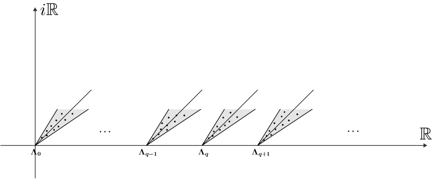
Similarly to Theorem 2.2, Fig. 1 illustrates graphically Theorem 2.4.

Fig. 1.
Illustration for the discrete spectrum generated near each LL by the potential V in Theorem 2.2.
Remark 2.4.
The above proof shows that in Theorem 2.4, $V = V_{ω} = Diag (ω W_{11}, ω W_{22})$ can be chosen such that $W_{j j}$ , $j = 1$ , 2, satisfy Assumptions 1.2(i)+(iv) and 2.2. In this case, if $W_{22}$ vanishes identically, then, (2.8) holds with $H_{V_{ω}} (b)$ replaced by $P_{V_{ω}} (b)$ .

Generalization to higher dimensions: Let $H_{0} (b_{1}, \dots, b_{d})$ , $d ⩾ 1$ , be the Schrödinger operators defined by (2.10), and $I_{2^{d}}$ denotes the $2^{d} \times 2^{d}$ identity matrix. Then, see [24] and [16, Identity (4.12)], the Pauli operators with constant magnetic fields of full rank essentially self-adjoint in $L^{2} (R^{2 d}, C^{2^{d}})$ , $d ⩾ 1$ , are originally defined on $C_{0}^{\infty} (R^{2 d}, C^{2^{d}})$ by $\begin{matrix} (2.20) & P_{0} (b_{1}, \dots, b_{d}) = H_{0} (b_{1}, \dots, b_{d}) I_{2^{d}} - Δ (b_{1}, \dots, b_{d}), \end{matrix}$ $Δ (b_{1}, \dots, b_{d})$ being the diagonal $2^{d} \times 2^{d}$ matrix having on the diagonal the sums $\sum_{j = 1}^{d} ε_{j} b_{j}$ , where $ε = (ε_{1}, \dots, ε_{d})$ belongs to the set ${(ε_{1}, \dots, ε_{d}) : all possible combinations of ε_{j} = \pm 1}$ . It is well-known, see for instance [16, Proposition 4.2], that the spectrum of the operator $P_{0} (b_{1}, \dots, b_{d})$ is given by the eigenvalues set of the PLLs with $\begin{matrix} (2.21) & σ (P_{0} (b_{1}, \dots, b_{d})) = σ_{ess} (P_{0} (b_{1}, \dots, b_{d})) = {2 \sum_{j = 1}^{d} b_{j} (q_{j} - 1) : (q_{1}, \dots, q_{d}) \in N^{d}} . \end{matrix}$ The Pauli operator $P_{0} (b)$ defined by (1.7) we consider corresponds to the case $d = 1$ and $b_{1} = b$ . However, in view of [16, Proposition 7.1], Theorems 2.3, 2.4 and Corollary 2.1 remain valid for the general Pauli operators in $L^{2} (R^{2 d}, C^{2^{d}})$ , $d ⩾ 1$ , defined by (2.20). More precisely:

In (1.15), the matrix $V = {V_{j k} (x)}_{j, k = 1}^{2^{d}}$ should be of size $2^{d}$ , $d ⩾ 1$ , $x = (x_{1}, y_{1}, \dots, x_{d}, y_{d}) \in R^{2 d}$ .

In Assumptions 1.2(ii)–(iii)–(iv), $R^{2}$ should be replaced by $R^{2 d}$ .

In Theorems 2.3, 2.4 and Corollary 2.1, p should satisfy $p ⩾ 2$ for $d = 1$ and $p > d$ for $d > 1$ . This condition is the one we need to impose to get the analogous of Proposition 3.2 in the general case.

In Theorem 2.4, the coefficients of the non-hermitian matrix-valued potential V should satisfy $V_{j k} \in L^{\infty} (R^{2 d}) \cap L^{p / 2} (R^{2 d})$ , $1 ⩽ j, k ⩽ 2^{d}$ .
2.2.2. The Dirac case

We recall that $P_{q}^{\pm}$ denotes the orthogonal projection onto $Ker (D_{0} (b) - Λ_{q}^{\pm})$ , where $Λ_{q}^{-} = - \sqrt{2 b q + 1}$ , $q \in N^{*}$ , and $Λ_{q}^{+} = \sqrt{2 b q + 1}$ , $q \in N$ , are the DLLs. Let V satisfy Assumptions 1.2(i)–(ii)–(iii) and 2.2, or Assumptions 1.2(i)+(iv) and 2.2. Then, we have $\begin{matrix} (2.22) & \sqrt{| W |} P_{q}^{\pm} = (Λ_{q}^{\pm} - λ) \sqrt{| W |} {(D_{0} (b) - λ)}^{- 1} P_{q}^{\pm} \in S_{p} \subset S_{\infty}, p > 2, \end{matrix}$ by Proposition 3.3, for $λ \in ρ (D_{0} (b))$ . Near a fixed DLL $Λ_{q}^{\pm}$ , $q ⩾ 0$ , the eigenvalues of the operator $D_{V} (b)$ can be parametrized by $λ_{q}^{\pm} = λ_{q}^{\pm} (k) : = Λ_{q}^{\pm} - k$ , with k small enough, see Section 4 for more details. As above, we define the counting function $\begin{matrix} (2.23) & N_{q, D_{V} (b)}^{\pm} (s, s_{0}) : = # {λ_{q}^{\pm} (k) \in σ_{disc} (D_{V} (b)) : s < | k | < s_{0}}, \end{matrix}$ for a fixed DLL. Under the above considerations, we establish the following theorem:

Theorem 2.5.
Let $V = V_{ω}$ satisfy Assumptions 1.2 (i)–(ii)–(iii) and 2.2 , with $p > 2$ , or Assumptions 1.2 (i)+(iv) and 2.2 . Fix a DLL $Λ_{q}^{\pm}$ . Then, there exists a discrete set $Σ_{q}^{\pm} \subset C^{}$ such that for all* $ω \in C^{} ∖ Σ_{q}^{\pm}$ , the operator* $D_{V_{ω}} (b)$ satisfies the following: there exists $r_{0} > 0$ such that:
$λ_{q}^{\pm} = λ_{q}^{\pm} (k) \in σ_{disc} (D_{V_{ω}} (b))$ , $| ω | r < | k | < | ω | r_{0}$ , satisfies $\begin{matrix} (2.24) & λ_{q}^{\pm} \in Λ_{q}^{\pm} + \tilde{ω} \overline{S (δ, r, r_{0})}, δ > 0, \end{matrix}$ where $S (δ, r, r_{0})$ is the sector defined by ( 2.3 ), and $\tilde{ω} : = \pm ω$ w.r.t. $\pm W ⩾ 0$ .

Suppose moreover that $rank (P_{q}^{\pm} | W | P_{q}^{\pm}) = \infty$ . Then, the number of eigenvalues of $D_{V_{ω}} (b)$ near $Λ_{q}^{\pm}$ is infinite. Furthermore, there exists a positive sequence ${(γ_{ℓ})}_{ℓ}$ tending to zero such that $\begin{matrix} (2.25) & lim_{ℓ ⟶ \infty} \frac{N_{q, D_{V_{ω}} (b)}^{\pm} (| ω | γ_{ℓ}, | ω | r_{0})}{Tr 1_{[γ_{ℓ}, \infty)} (P_{q}^{\pm} | W | P_{q}^{\pm})} = 1 . \end{matrix}$

Now, let V satisfy Assumptions 1.2(i)+(iv) and 2.2 with $W = Diag (U, U) = U I_{2}$ . Then, by [16, Proposition 8.1], the Toeplitz operator $P_{q}^{\pm} | W | P_{q}^{\pm}$ , $q ⩾ 0$ , obeys up to a multiplicative explicit constant, the asymptotic $\begin{matrix} (2.26) & Tr 1_{[r, \infty)} (P_{q}^{\pm} | W | P_{q}^{\pm}) \sim \frac{| ln r |}{ln | ln r |} as r ↘ 0 . \end{matrix}$ Therefore, this together with Theorem 2.5 give the following corollary:
Corollary 2.2.
Let $V = V_{ω}$ satisfy Assumptions 1.2 (i)+(iv) and 2.2 . Assume moreover that $W = Diag (U, U)$ . Then, in Theorem 2.5 , for $ω \in C^{} ∖ Σ_{q}^{\pm}$ , the number of eigenvalues of* $D_{V_{ω}} (b)$ near $Λ_{q}^{\pm}$ is infinite, and there exists a positive sequence ${(γ_{ℓ})}_{ℓ}$ tending to zero such that $N_{q, D_{V_{ω}} (b)}^{\pm} (| ω | γ_{ℓ}, | ω | r_{0})$ satisfies ( 2.25 ).
Remark 2.5.

Theorem 2.5 remains valid if the condition $ω \in C^{} ∖ Σ_{q}^{\pm}$ is replaced by ω small enough.

In Corollary 2.2, since $| W |$ is compactly supported, then, the eigenvalues of the operator $D_{V_{ω}} (b)$ satisfy near the DLL $Λ_{q}^{\pm}$ $\begin{matrix} (2.27) & lim_{r ↘ 0} \frac{N_{q, D_{V_{ω}} (b)}^{\pm} (| ω | r, | ω | r_{0})}{Tr 1_{[r, \infty)} (P_{q}^{\pm} | W | P_{q}^{\pm})} = 1 . \end{matrix}$

A consequence of Theorem 2.5 and Corollary 2.2 is the following result:
Theorem 2.6.
Let* $p > 2$ . Then, there exists a non-hermitian matrix-valued potential $V = {V_{j k} (x)}_{j, k = 1}^{2}$ , with $V_{j k} \in L^{\infty} (R^{2}) \cap L^{p / 2} (R^{2})$ decaying at infinity, generating near each DLL $Λ_{q}^{\pm}$ , $q ⩾ 0$ , infinitely many eigenvalues lying in $σ_{disc} (D_{V} (b))$ , which are located near a semi-axis of origin $Λ_{q}^{\pm}$ .
Proof.
According to Theorem 2.5 and Corollary 2.2, it suffices to consider any matrix-valued potential $V = V_{ω} = Diag (ω U, ω U)$ satisfying Assumptions 1.2(i)+(iv) and 2.2, with $ω \in C^{} ∖ (R^{} \cup (⋃_{q}^{\infty} Σ_{q}^{\pm}))$ . □

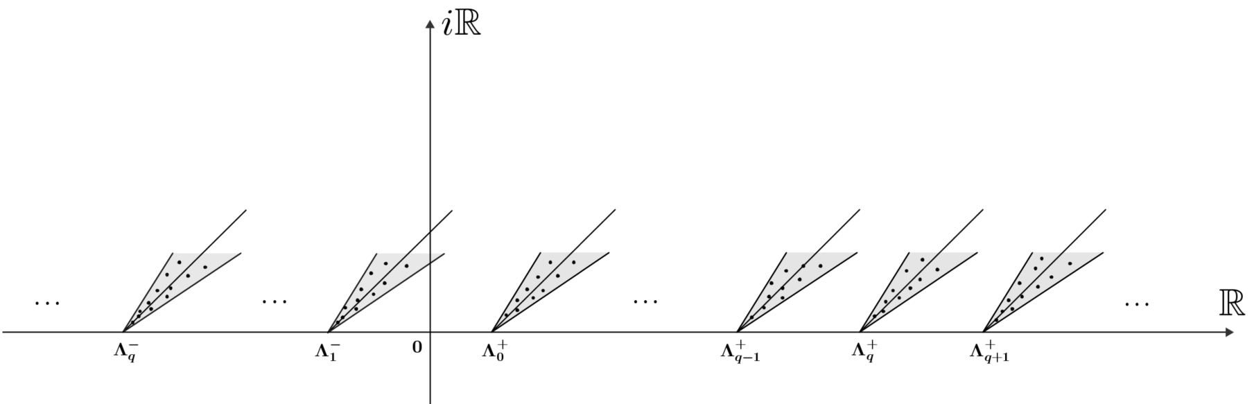
We refer to Fig. 2 for a graphic illustration of Theorem 2.6.

Fig. 2.
Illustration for the discrete spectrum generated near each DLL by the potential V in Theorem 2.6.
Remark 2.6.
As shows the above proof, in Theorem 2.6, V can be chosen of the form $V = V_{ω} = Diag (ω U, ω U)$ , compactly supported satisfying Assumptions 1.2(i)+(iv) and 2.2. In this case, according to [16, Proposition 8.1] together with Remark 2.5(b), we have up to a multiplicative explicit constant, $\begin{matrix} (2.28) & N_{q, D_{V_{ω}} (b)} (| ω | r, | ω | r_{0}) \sim \frac{| ln r |}{ln | ln r |}, r ↘ 0 . \end{matrix}$ In particular, this shows how the (complex) eigenvalues converge to the DLLs asymptotically. Hence, Theorem 2.6 can be reformulated in such a way we have a non-self-adjoint extension of Melgaard–Rozenblum [16, Theorem 1.3] (for $d = 1$ ).

Generalization to higher dimensions: To define the Dirac operators with constant magnetic fields of full rank in higher dimensions $2 d$ , $d ⩾ 1$ , we refer for instance to the description given in [16, Section 4] and [24] for more details. For a given $d ⩾ 1$ , let $σ_{1}^{(d)}, \dots, σ_{2 d}^{(d)}, σ_{0}^{(d)}$ be the $2 d + 1$ Dirac matrices of size $2^{d}$ , governed, as in (1.6), by the relations $\begin{matrix} (2.29) & {(σ_{j}^{(d)})}^{*} = σ_{j}^{(d)} and σ_{j}^{(d)} σ_{k}^{(d)} + σ_{k}^{(d)} σ_{j}^{(d)} = 2 δ_{j k} I_{2^{d}}, 0 ⩽ j, k ⩽ 2 d, \end{matrix}$ where $I_{2^{d}}$ denotes the $2^{d} \times 2^{d}$ identity matrix. For $b_{j} \in R$ , $1 ⩽ j ⩽ d$ , $(x_{1}, y_{1}, \dots, x_{d}, y_{d}) \in R^{2 d}$ , introduce the operators $P_{2 j - 1} = (- i \partial_{x_{j}} + \frac{b_{j} y_{j}}{2})$ and $P_{2 j} = (- i \partial_{y_{j}} - \frac{b_{j} x_{j}}{2})$ . Then, the Dirac operators with constant magnetic fields of full rank essentially self-adjoint in $L^{2} (R^{2 d}, C^{2^{d}})$ , $d ⩾ 1$ , are originally defined on $C_{0}^{\infty} (R^{2 d}, C^{2^{d}})$ by $\begin{matrix} (2.30) & D_{0} (b_{1}, \dots, b_{d}) = \sum_{j = 1}^{2 d} σ_{j}^{(d)} P_{j} + σ_{0}^{(d)} . \end{matrix}$ It is well-known, see for instance [16], that the spectrum of the operator $D_{0} (b_{1}, \dots, b_{d})$ is given by the eigenvalues set of the DLLs with $\begin{matrix} (2.31) & σ (D_{0} (b_{1}, \dots, b_{d})) = σ_{ess} (D_{0} (b_{1}, \dots, b_{d})) = {\pm \sqrt{I_{q} + 1} : q = (q_{1}, \dots, q_{d}) \in N^{d}}, \end{matrix}$ where $I_{q}$ can be expressed as $I_{q} = 2 \sum_{j = 1}^{d} | b_{j} | (q_{j} - 1)$ . Note that in (2.31), the symmetry of $\pm \sqrt{I_{q} + 1}$ breaks down for the “lowest” DLL $\pm \sqrt{I_{0} + 1} = \pm 1$ corresponding to $q = (1, \dots, 1)$ . It is either 1 or $- 1$ . The Dirac operator $D_{0} (b)$ defined by (1.10) we consider corresponds to the case $d = 1$ and $b_{1} = b$ . However, Theorems 2.5 remains valid for the general Dirac operators in $L^{2} (R^{2 d}, C^{2^{d}})$ , $d ⩾ 1$ , defined by (2.30). Furthermore, in view of [16, Proposition 8.1], Corollary 2.2 and Theorem 2.6 remain also valid for the Dirac operators (2.30). More precisely:

In (1.15), the matrix $V = {V_{j k} (x)}_{j, k = 1}^{2^{d}}$ should be of size $2^{d}$ , $d ⩾ 1$ , $x = (x_{1}, y_{1}, \dots, x_{d}, y_{d}) \in R^{2 d}$ .

In Assumptions 1.2(ii)–(iii)–(iv), $R^{2}$ should be replaced by $R^{2 d}$ .

In Theorems 2.5, 2.6 and Corollary 2.2, p should satisfy $p > 2 d$ for $d ⩾ 1$ . The condition $p > 2 d$ , $d ⩾ 1$ above, is the one we need to impose to get the analogous of Proposition 3.3 in the general case.

In Theorem 2.6, the coefficients of the non-hermitian matrix-valued potential V should satisfy $V_{j k} \in L^{\infty} (R^{2 d}) \cap L^{p / 2} (R^{2 d})$ , $1 ⩽ j, k ⩽ 2^{d}$ .

In Remark 2.6, according to [16, Proposition 8.1], (2.28) will take the more general form $\begin{matrix} (2.32) & N_{q, D_{V_{ω}} (b)} (| ω | r, | ω | r_{0}) \sim \frac{1}{d!} {(\frac{| ln r |}{ln | ln r |})}^{d}, r ↘ 0, \end{matrix}$ up to a multiplicative explicit constant given by (4.17) of [16].
3. Schatten–von Neumann bounds

In this section, we establish useful Schatten–von Neumann bounds implying in particular the relatively compactness of the potential perturbation w.r.t. the free operators. We conserve the notations introduced above. Also, note that in the estimates or equalities appearing in the proofs below, the constants are generic, i.e. may change from an estimate or equality to another even if the same notation is used for simplification.

3.1. Bounds on Schrödinger operators

Proposition 3.1.

Let V be complex-valued satisfying Assumption 1.1 (ii), and $λ \in C ∖ ⋃_{q = 0}^{\infty} {Λ_{q}}$ . Then, $\sqrt{| V |} {(H_{0} (b) - λ)}^{- 1} \in S_{p}$ and there exists a constant $C_{p, b}$ depending only on $p ⩾ 2$ and b, such that $\begin{matrix} (3.1) & {‖ \sqrt{| V |} {(H_{0} (b) - λ)}^{- 1} ‖}_{S_{p}} ⩽ C_{p, b} ‖ \sqrt{G} ‖_{L^{p}} (1 + \frac{| λ + 1 |}{dist (λ, ⋃_{q = 0}^{\infty} {Λ_{q}})}) . \end{matrix}$

For $V \in L^{\infty} (R^{2})$ compactly supported, for each $p ⩾ 2$ , the same conclusion holds with $\sqrt{G}$ replaced by $\sqrt{| V |}$ in the r.h.s. of ( 3.1 ).
In particular, in both cases, V is relatively compact w.r.t. the operator $H_{0} (b)$ .
Proof.
(i) Due to Assumption 1.1(ii), there exists a bounded operator $B$ on $L^{2} (R^{2})$ such that $\sqrt{| V |} = B \sqrt{G}$ . Thus, $‖ \sqrt{| V |} {(H_{0} (b) - λ)}^{- 1} ‖_{S_{p}} ⩽ C ‖ \sqrt{G} {(H_{0} (b) - λ)}^{- 1} ‖_{S_{p}}$ for some constant $C > 0$ . Since $\sqrt{G} \in L^{p} (R^{2})$ , then, to show the claim, it suffices to prove that for any $U \in L^{p} (R^{2})$ , we have the bound $\begin{matrix} (3.2) & {‖ U {(H_{0} (b) - λ)}^{- 1} ‖}_{S_{p}} ⩽ C_{p, b} ‖ U ‖_{L^{p}} (1 + \frac{| λ + 1 |}{dist (λ, ⋃_{q = 0}^{\infty} {Λ_{q}})}) . \end{matrix}$

(a) Firstly, we shall prove (3.2) for p even. To prove the general case, we shall use an interpolation argument. Let p be even. We have $\begin{matrix} (3.3) & {‖ U {(H_{0} (b) - λ)}^{- 1} ‖}_{S_{p}} ⩽ {‖ U {(H_{0} (b) + 1)}^{- 1} ‖}_{S_{p}} ‖ (H_{0} (b) + 1) {(H_{0} (b) - λ)}^{- 1} ‖ . \end{matrix}$ The spectral mapping theorem yields $\begin{matrix} (3.4) & ‖ (H_{0} (b) + 1) {(H_{0} (b) - λ)}^{- 1} ‖ ⩽ sup_{ϱ \in σ (H_{0} (b))} | \frac{ϱ + 1}{ϱ - λ} | ⩽ (1 + \frac{| λ + 1 |}{dist (λ, ⋃_{q = 0}^{\infty} {Λ_{q}})}) . \end{matrix}$ The diamagnetic inequality, see for instance [2, Theorem 2.3] and [25, Theorem 2.13], implies that there exists a constant $C > 0$ such that $\begin{array}{l} {‖ U {(H_{0} (b) + 1)}^{- 1} ‖}_{S_{p}} \\ = {‖ U {({(- i \nabla - A)}^{2} - b + 1)}^{- 1} ‖}_{S_{p}} \\ ⩽ {‖ U {({(- i \nabla - A)}^{2} + 1)}^{- 1} ‖}_{S_{p}} ‖ ({(- i \nabla - A)}^{2} + 1) {({(- i \nabla - A)}^{2} - b + 1)}^{- 1} ‖ \\ = {‖ U {({(- i \nabla - A)}^{2} + 1)}^{- 1} ‖}_{S_{p}} ‖ I + {(H_{0} (b) + 1)}^{- 1} b ‖ \\ (3.5) & ⩽ C {‖ U {(- Δ + 1)}^{- 1} ‖}_{S_{p}} C_{b} = C_{b} {‖ U {(- Δ + 1)}^{- 1} ‖}_{S_{p}} . \end{array}$ Now, since p is even, then, by the standard criterion [25, Theorem 4.1], it follows that $\begin{matrix} (3.6) & {‖ U {(- Δ + 1)}^{- 1} ‖}_{S_{p}} ⩽ C ‖ U ‖_{L^{p}} {‖ {(| \cdot |^{2} + 1)}^{- 1} ‖}_{L^{p}} . \end{matrix}$ Thus, estimate (3.2), for p even, follows by putting together bounds (3.3), (3.4), (3.5) and (3.6).

(b) Let us show now that (3.2) is true for each $p ⩾ 2$ . For any $p > 2$ , there exists even integers $p_{0} < p_{1}$ such that $p \in (p_{0}, p_{1})$ with $p_{0} ⩾ 2$ . Let $γ \in (0, 1)$ with $\frac{1}{p} = \frac{1 - γ}{p_{0}} + \frac{γ}{p_{1}}$ , and consider the operator $\begin{matrix} L^{p_{i}} (R^{2}) ∋ U \overset{M}{⟼} U {(H_{0} (b) - λ)}^{- 1} \in S_{p_{i}}, i = 0, 1 . \end{matrix}$ For $i = 0$ , 1, let $C_{i} = C_{p_{i}, b}$ denote the constant appearing in (3.2), and define $\begin{matrix} C_{λ, p_{i}, b} : = C_{i} (1 + \frac{| λ + 1 |}{dist (λ, ⋃_{q = 0}^{\infty} {Λ_{q}})}) . \end{matrix}$ Bound (3.2) implies that $‖ M ‖ ⩽ C_{λ, p_{i}, b}$ for $i = 0$ , 1. By using the Riesz–Thorin Theorem, see for instance [8, Sub. 5 of Chap. 6], [21,26], [15, Chap. 2], we can interpolate between $p_{0}$ and $p_{1}$ to obtain the extension $M : L^{p} (R^{2}) ⟶ S_{p}$ , with $\begin{matrix} ‖ M ‖ ⩽ C_{λ, p_{0}, b}^{1 - γ} C_{λ, p_{1}, b}^{γ} ⩽ C_{p, b} (1 + \frac{| λ + 1 |}{dist (λ, ⋃_{q = 0}^{\infty} {Λ_{q}})}) . \end{matrix}$ Therefore, for any $U \in L^{p} (R^{2})$ , we have $\begin{matrix} {‖ M (U) ‖}_{S_{p}} ⩽ C_{p, b} (1 + \frac{| λ + 1 |}{dist (λ, ⋃_{q = 0}^{\infty} {Λ_{q}})}) ‖ U ‖_{L^{p}}, \end{matrix}$ or equivalently estimate (3.2).

(ii) For $V \in L^{\infty} (R^{2})$ compactly supported, $\sqrt{| V |} \in L^{p} (R^{2})$ for each $p ⩾ 2$ . Thus, the claim follows according to (3.2). This concludes the proof of the proposition. □
3.2. Bounds on Pauli and Dirac operators

Concerning the Pauli operator, we have the following proposition:

Proposition 3.2.

Let V be non-hermitian matrix-valued satisfying Assumption 1.2 (ii), and $λ \in C ∖ ⋃_{q = 0}^{\infty} {Λ_{q}}$ . Then, $\sqrt{| V |} {(P_{0} (b) - λ)}^{- 1} \in S_{p}$ and there exists a constant $C_{p, b}$ depending only on $p ⩾ 2$ and b, such that $\begin{matrix} (3.7) & {‖ \sqrt{| V |} {(P_{0} (b) - λ)}^{- 1} ‖}_{S_{p}} ⩽ C_{p, b} ‖ \sqrt{G} ‖_{L^{p}} (1 + \frac{| λ + 1 |}{dist (λ, ⋃_{q = 0}^{\infty} {Λ_{q}})}) . \end{matrix}$

Assume that V does not vanish identically and the coefficients $V_{j k}$ that do not vanish identically satisfy $V_{j k} \in L^{\infty} (R^{2})$ and compactly supported. Then, for each $p ⩾ 2$ , ( 3.7 ) holds with $\sqrt{G}$ replaced by $e^{- κ | x |}$ , $κ > 0$ .
In particular, in both cases, V is relatively compact w.r.t. the operator $P_{0} (b)$ .
Proof.
It is left to the reader since the use of the identity (1.8) allows to mimic easily the proof of Proposition 3.1. Note that for V and the $V_{j k}$ as in (ii), Assumption 1.2(ii) holds with $G = C e^{- 2 κ | x |}$ , $κ > 0$ , for some constant $C > 0$ . □

For the Dirac operator, we have the following result: Proposition 3.3.

Let V satisfy Assumption 1.2 (ii) and $λ \in C ∖ ({⋃_{q = 1}^{\infty} {Λ_{q}^{-}}} \cup {⋃_{q = 0}^{\infty} {Λ_{q}^{+}}})$ . Then, $\sqrt{| V |} {(D_{0} (b) - λ)}^{- 1} \in S_{p}$ and there exists a constant $C_{p, b}$ depending only on $p > 2$ and b, such that $\begin{matrix} (3.8) & {‖ \sqrt{| V |} {(D_{0} (b) - λ)}^{- 1} ‖}_{S_{p}} ⩽ C_{p, b} ‖ \sqrt{G} ‖_{L^{p}} (1 + (| λ | + | λ |^{2}) (2 + C_{1} (λ) + C_{2} (λ))), \end{matrix}$ where we have set $\begin{matrix} (3.9) & C_{1} (λ) : = \frac{| λ |^{2}}{dist (λ^{2}, ⋃_{q = 0}^{\infty} {Λ_{q} + 1})} and C_{2} (λ) : = \frac{| λ |^{2}}{dist (λ^{2}, ⋃_{q = 0}^{\infty} {Λ_{q} + 2 b + 1})}, \end{matrix}$ $Λ_{q}$ , $q ⩾ 0$ , being the LLs of the Schrödinger operator $H_{0} (b)$ .

Assume that V does not vanish identically and the coefficients $V_{j k}$ that do not vanish identically satisfy $V_{j k} \in L^{\infty} (R^{2})$ and compactly supported. Then, for each $p ⩾ 2$ , ( 3.8 ) holds with $\sqrt{G}$ replaced by $e^{- κ | x |}$ , $κ > 0$ .
In particular, in both cases, V is relatively compact w.r.t. the operator $D_{0} (b)$ .
Proof.
Since in the second point (ii) Assumption 1.2(ii) holds with $G = C e^{- 2 κ | x |}$ , $κ > 0$ , for some constant $C > 0$ , then, it suffices to prove only (i). Let $λ \in C ∖ ({⋃_{q = 1}^{\infty} {Λ_{q}^{-}}} \cup {⋃_{q = 0}^{\infty} {Λ_{q}^{+}}})$ , the resolvent set of the operator $D_{0} (b)$ . We have $\begin{matrix} (3.10) & {(D_{0} (b) - λ)}^{- 1} = D_{0} {(b)}^{- 1} + λ (1 + λ D_{0} {(b)}^{- 1}) {(D_{0} {(b)}^{2} - λ^{2})}^{- 1} . \end{matrix}$ By setting $\begin{matrix} (3.11) & T_{1} (λ) : = λ (1 + λ D_{0} {(b)}^{- 1}) {(D_{0} {(b)}^{2} - λ^{2})}^{- 1}, \end{matrix}$ it follows from (3.10) that $\begin{matrix} (3.12) & \sqrt{| V |} {(D_{0} (b) - λ)}^{- 1} = \sqrt{| V |} D_{0} {(b)}^{- 1} + \sqrt{| V |} T_{1} (λ) . \end{matrix}$ Due to Assumption 1.2(ii), there exists a bounded operator $B$ on $L^{2} (R^{2})$ such that $\sqrt{| V |} = B \sqrt{G}$ . Thus, it follows from (3.12) that there exists a constant $C > 0$ such that $\begin{matrix} (3.13) & {‖ \sqrt{| V |} {(D_{0} (b) - λ)}^{- 1} ‖}_{S_{p}} ⩽ C {‖ \sqrt{G} {| D_{0} (b) |}^{- 1} ‖}_{S_{p}} + C {‖ \sqrt{G} T_{1} (λ) ‖}_{S_{p}} . \end{matrix}$

(a) Firstly, we estimate the second term of the r.h.s. of (3.13). Using (3.11), we find that there exists a constant $C > 0$ such that $\begin{matrix} (3.14) & {‖ \sqrt{G} T_{1} (λ) ‖}_{S_{p}} ⩽ C (| λ | + | λ |^{2}) {‖ \sqrt{G} {(D_{0} {(b)}^{2} - λ^{2})}^{- 1} ‖}_{S_{p}} . \end{matrix}$ This together with the identity (1.11) implies that $\begin{array}{l} {‖ \sqrt{G} T_{1} (λ) ‖}_{S_{p}} \\ (3.15) & ⩽ C (| λ | + | λ |^{2}) ({‖ \sqrt{G} {(H_{0} (b) + 1 - λ^{2})}^{- 1} ‖}_{S_{p}} + {‖ \sqrt{G} {(H_{0} (b) + 2 b + 1 - λ^{2})}^{- 1} ‖}_{S_{p}}) . \end{array}$ We have $\begin{matrix} (3.16) & {‖ \sqrt{G} {(H_{0} (b) + 1 - λ^{2})}^{- 1} ‖}_{S_{p}} ⩽ {‖ \sqrt{G} {(H_{0} (b) + 1)}^{- 1} ‖}_{S_{p}} ‖ (H_{0} (b) + 1) {(H_{0} (b) + 1 - λ^{2})}^{- 1} ‖ . \end{matrix}$ Since $σ (H_{0} (b) + 1) = ⋃_{q = 0}^{\infty} {Λ_{q} + 1}$ , then, the spectral mapping theorem implies that $\begin{array}{l} ‖ (H_{0} (b) + 1) {(H_{0} (b) + 1 - λ^{2})}^{- 1} ‖ \\ (3.17) & ⩽ sup_{ϱ \in σ (H_{0} (b) + 1)} | \frac{ϱ}{ϱ - λ^{2}} | ⩽ (1 + \frac{| λ |^{2}}{dist (λ^{2}, ⋃_{q = 0}^{\infty} {Λ_{q} + 1})}) . \end{array}$ Thus, reasoning as in the proof of Proposition 3.1, it can be shown by using (3.16), the diamagnetic inequality, the standard criterion [25, Theorem 4.1] and the interpolation argument, that $\begin{matrix} (3.18) & {‖ \sqrt{G} {(H_{0} (b) + 1 - λ^{2})}^{- 1} ‖}_{S_{p}} ⩽ C_{p, b} ‖ \sqrt{G} ‖_{L^{p}} (1 + \frac{| λ |^{2}}{dist (λ^{2}, ⋃_{q = 0}^{\infty} {Λ_{q} + 1})}) . \end{matrix}$ Similarly, we have $\begin{array}{l} {‖ \sqrt{G} {(H_{0} (b) + 2 b + 1 - λ^{2})}^{- 1} ‖}_{S_{p}} \\ (3.19) & ⩽ {‖ \sqrt{G} {(H_{0} (b) + 2 b + 1)}^{- 1} ‖}_{S_{p}} ‖ (H_{0} (b) + 2 b + 1) {(H_{0} (b) + 2 b + 1 - λ^{2})}^{- 1} ‖ . \end{array}$ Since $σ (H_{0} (b) + 2 b + 1) = ⋃_{q = 0}^{\infty} {Λ_{q} + 2 b + 1}$ , then, the spectral mapping theorem implies that $\begin{array}{l} ‖ (H_{0} (b) + 2 b + 1) {(H_{0} (b) + 2 b + 1 - λ^{2})}^{- 1} ‖ \\ (3.20) & ⩽ sup_{ϱ \in σ (H_{0} (b) + 2 b + 1)} | \frac{ϱ}{ϱ - λ^{2}} | ⩽ (1 + \frac{| λ |^{2}}{dist (λ^{2}, ⋃_{q = 0}^{\infty} {Λ_{q} + 2 b + 1})}) . \end{array}$ Thus, reasoning as in the proof of Proposition 3.1, it can be shown by using (3.19), the diamagnetic inequality, the standard criterion [25, Theorem 4.1] and the interpolation argument, that $\begin{matrix} (3.21) & {‖ \sqrt{G} {(H_{0} (b) + 2 b + 1 - λ^{2})}^{- 1} ‖}_{S_{p}} ⩽ C_{p, b} ‖ \sqrt{G} ‖_{L^{p}} (1 + \frac{| λ |^{2}}{dist (λ^{2}, ⋃_{q = 0}^{\infty} {Λ_{q} + 2 b + 1})}) . \end{matrix}$ By putting together bounds (3.15), (3.18) and (3.21), we get $\begin{matrix} (3.22) & {‖ \sqrt{G} T_{1} (λ) ‖}_{S_{p}} ⩽ C_{p, b} ‖ \sqrt{G} ‖_{L^{p}} (| λ | + | λ |^{2}) (2 + C_{1} (λ) + C_{2} (λ)), \end{matrix}$ where $C_{1} (λ)$ and $C_{2} (λ)$ are defined by (3.9).

(b) Now, we estimate the first term $‖ \sqrt{G} | D_{0} (b) |^{- 1} ‖_{S_{p}}$ of the r.h.s. of (3.13). Thanks to (1.11) and the identity $| D_{0} (b) |^{- α} = {(D_{0} {(b)}^{2})}^{- \frac{α}{2}}$ , $α > 0$ , it follows that $\begin{matrix} (3.23) & {‖ \sqrt{G} {| D_{0} (b) |}^{- α} ‖}_{S_{p}} ⩽ ({‖ \sqrt{G} {(H_{0} (b) + 1)}^{- \frac{α}{2}} ‖}_{S_{p}} + {‖ \sqrt{G} {(H_{0} (b) + 2 b + 1)}^{- \frac{α}{2}} ‖}_{S_{p}}) . \end{matrix}$ Thus, as in the proof of a) above, the use of the diamagnetic inequality, the standard criterion [25, Theorem 4.1] and the interpolation argument, allows to show that for $α p > 2$ , each term of the r.h.s. of (3.23) is bounded by $C_{p, b, α} ‖ \sqrt{G} ‖_{L^{p}}$ , where $C_{p, b, α} > 0$ is a constant depending only on p, b and α. In particular, for $α = 1$ , we obtain $\begin{matrix} (3.24) & {‖ \sqrt{G} {| D_{0} (b) |}^{- 1} ‖}_{S_{p}} ⩽ C_{p, b} ‖ \sqrt{G} ‖_{L^{p}} . \end{matrix}$ This together with bounds (3.13) and (3.22) give the proposition. □

4. Analytic interpretations of the discrete eigenvalues problem

For further use, let us recall some useful concepts by following [11, Section 4]. Let $H$ be a Hilbert space as above. We denote $L (H)$ (resp. $GL (H)$ ) the set of bounded (resp. invertible) operators in $H$ .

Definition 4.1.
Let $U$ be a neighbourhood of a fixed point $w \in C$ , and $F : U ∖ {w} ⟶ L (H)$ be a holomorphic operator-valued function. The function F is said to be finite meromorphic at w if its Laurent expansion at w has the form $F (z) = \sum_{n = m}^{+ \infty} {(z - w)}^{n} A_{n}$ , $m > - \infty$ , where (if $m < 0$ ) the operators $A_{m}, \dots, A_{- 1}$ are of finite rank. Moreover, if $A_{0}$ is a Fredholm operator, then, the function F is said to be Fredholm at w. In this case, the Fredholm index of $A_{0}$ is called the Fredholm index of F at w.
Proposition 4.1 ([11, Proposition 4.1.4]).

Let $D \subseteq C$ be a connected open set, $Z \subseteq D$ be a closed and discrete subset of $D$ , and $F : D ⟶ L (H)$ be a holomorphic operator-valued function in $D ∖ Z$ . Assume that F is finite meromorphic on $D$ (i.e. it is finite meromorphic near each point of Z), F is Fredholm at each point of $D$ , and there exists $w_{0} \in D ∖ Z$ such that $F (w_{0})$ is invertible. Then, there exists a closed and discrete subset $Z^{'}$ of $D$ such that $Z \subseteq Z^{'}$ , $F (z)$ is invertible for each $z \in D ∖ Z^{'}$ , $F^{- 1} : D ∖ Z^{'} ⟶ GL (H)$ is finite meromorphic and Fredholm at each point of $D$ .

In the setting of Proposition 4.1, we define the characteristic values of F and their multiplicities as follows:

Definition 4.2.
The points of $Z^{'}$ where the function F or $F^{- 1}$ is not holomorphic are called the characteristic values of F. The multiplicity of a characteristic value $w_{0}$ is defined by $\begin{matrix} (4.1) & mult (w_{0}) : = \frac{1}{2 i π} Tr \int_{| w - w_{0} | = ρ} F^{'} (z) F {(z)}^{- 1} d z, \end{matrix}$ where $ρ > 0$ is chosen small enough so that ${w \in C : | w - w_{0} | ⩽ ρ} \cap Z^{'} = {w_{0}}$ .

According to Definition 4.2, if the function F is holomorphic in $D$ , then, the characteristic values of F are just the complex numbers w where the operator $F (w)$ is not invertible. Then, results of [12] and [11, Section 4] imply that $mult (w)$ is an integer. Let $Ω \subseteq D$ be a connected domain with boundary $\partial Ω$ not intersecting $Z^{'}$ . The sum of the multiplicities of the characteristic values of the function F lying in Ω is called the index of F w.r.t. the contour $\partial Ω$ and is defined by $\begin{matrix} (4.2) & {Ind}_{\partial Ω} F : = \frac{1}{2 i π} Tr \int_{\partial Ω} F^{'} (z) F {(z)}^{- 1} d z = \frac{1}{2 i π} Tr \int_{\partial Ω} F {(z)}^{- 1} F^{'} (z) d z . \end{matrix}$

In order to simplify the presentation and to shorten the article, we will treat simultaneously the three Hamiltonians. Hence, we recall that $H_{V} (b)$ denotes the operators $H_{V} (b)$ , $P_{V} (b)$ and $D_{V} (b)$ . Thus, by (1.3), (1.9) and (1.13), we have $\begin{matrix} (4.3) & σ (H_{0} (b)) = σ_{ess} (H_{0} (b)) = \{\begin{matrix} ⋃_{q = 0}^{\infty} {Λ_{q}} & if H_{0} (b) = H_{0} (b) or P_{0} (b), \\ {⋃_{q = 1}^{\infty} {Λ_{q}^{-}}} \cup {⋃_{q = 0}^{\infty} {Λ_{q}^{+}}} & if H_{0} (b) = D_{0} (b), \end{matrix} \end{matrix}$ where $Λ_{q} = 2 b q$ and $Λ_{q}^{\pm} = \pm \sqrt{2 b q + 1}$ are the DLPLs. In the sequel, w.r.t. (4.3), we will write $\begin{matrix} σ (H_{0} (b)) = σ_{ess} (H_{0} (b)) = ⋃_{q = 0}^{\infty} {Λ_{q}^{#}} . \end{matrix}$ $P_{q}^{#}$ , $q ⩾ 0$ , will denote the orthogonal projection onto $Ker (H_{0} (b) - Λ_{q}^{#})$ , and $Q_{q}^{#}$ , $q ⩾ 0$ , will denote the orthogonal projection onto $⋃_{j \neq q} Ker (H_{0} (b) - Λ_{j}^{#})$ . Thus, $Q_{q}^{#} = I - P_{q}^{#}$ .

For a fixed spectral threshold $Λ_{q}^{#} \in ⋃_{q = 0}^{\infty} {Λ_{q}}$ , let $\begin{matrix} (4.4) & 0 < ε < 2 b . \end{matrix}$ In the case $Λ_{q}^{#} = Λ_{q}^{\pm} \in {⋃_{q = 1}^{\infty} {Λ_{q}^{-}}} \cup {⋃_{q = 0}^{\infty} {Λ_{q}^{+}}}$ fixed, we impose that $\begin{matrix} (4.5) & 0 < ε < \{\begin{matrix} \sqrt{2 b + 1} - 1 & for q = 0, \\ min (Λ_{q}^{#} - Λ_{-}, Λ_{+} - Λ_{q}^{#}) & for q ⩾ 1, \end{matrix} \end{matrix}$ where $Λ_{\pm}$ denote the DLLs respectively on the right and the left on $Λ_{q}^{#}$ . Hence, we define $D_{q} {(ε)}^{} : = {λ \in C : 0 < | Λ_{q}^{#} - λ | < ε}$ . Put the change of variables $Λ_{q}^{#} - λ = k$ and introduce $D {(0, ε)}^{} : = {k \in C : 0 < | k | < ε}$ . Thus, $D_{q} {(ε)}^{}$ can be parametrized by $\begin{matrix} (4.6) & λ = λ_{q} (k) : = Λ_{q}^{#} - k, k \in D {(0, ε)}^{}, \end{matrix}$ and we have the relation $D_{q} {(ε)}^{} = Λ_{q}^{#} + D {(0, ε)}^{}$ . We have the following proposition:
Proposition 4.2.
Let $V = V_{ω}$ satisfy the assumptions of Theorems 2.1 , 2.3 or 2.5 . Then, for any fixed spectral threshold $Λ_{q}^{#}$ , $q ⩾ 0$ , the operator-valued function $\begin{matrix} D {(0, ε)}^{} ∋ k ⟼ T_{V_{ω}} (λ_{q} (k)) : = \pm ω \sqrt{| W |} {(H_{0} (b) - λ_{q} (k))}^{- 1} \sqrt{| W |} \end{matrix}$ is analytic with values in the Schatten–von Neumann class* $S_{p}$ .
Proof.
Assume that $V = V_{ω}$ satisfy the assumptions of Theorems 2.1, 2.3 or 2.5. Then, thanks to Propositions 3.1, 3.2 and 3.3, together with $λ_{q} (k) \in ρ (H_{0} (b)) = C ∖ ⋃_{q = 0}^{\infty} {Λ_{q}^{#}}$ for $k \in D {(0, ε)}^{}$ , we have $T_{V_{ω}} (λ_{q} (k)) \in S_{p}$ .

Let us show the analyticity of the map $D {(0, ε)}^{} ∋ k ⟼ T_{V_{ω}} (λ_{q} (k))$ . We have, using (4.6), $\begin{array}{l} \sqrt{| W |} {(H_{0} (b) - λ_{q} (k))}^{- 1} \sqrt{| W |} \\ = \sqrt{| W |} P_{q}^{#} {(H_{0} (b) - λ_{q} (k))}^{- 1} \sqrt{| W |} + \sqrt{| W |} Q_{q}^{#} {(H_{0} (b) - λ_{q} (k))}^{- 1} \sqrt{| W |} \\ (4.7) & = k^{- 1} \sqrt{| W |} P_{q}^{#} \sqrt{| W |} + \sqrt{| W |} Q_{q}^{#} {(H_{0} (b) - λ_{q} (k))}^{- 1} \sqrt{| W |} . \end{array}$ Now, each term of the sum (4.7) is analytic in $D {(0, ε)}^{}$ . Then, so is the map $D {(0, ε)}^{} ∋ k ⟼ T_{V_{ω}} (λ_{q} (k))$ . This concludes the proof. □

Propositions 3.1, 3.2 and 3.3 imply that the operator $ω W {(H_{0} (b) - λ)}^{- 1}$ is of class $S_{p}$ , $p ⩾ 2$ , for $λ \in ρ (H_{0} (b))$ . Consequently, we can introduce the $⌈ p ⌉$ -regularized determinant $\begin{array}{l} {det}_{⌈ p ⌉} (I + ω W {(H_{0} (b) - λ)}^{- 1}) \\ (4.8) & : = det {(I + ω W {(H_{0} (b) - λ)}^{- 1}) exp (\sum_{k = 1}^{⌈ p ⌉ - 1} \frac{{(- ω W {(H_{0} (b) - λ)}^{- 1})}^{k}}{k})}, \end{array}$ where $⌈ p ⌉ : = min {n \in N : n ⩾ p}$ . It is well known, see for instance [25, Chap. 9], that we have the characterization $\begin{matrix} (4.9) & λ \in σ_{disc} (H_{V_{ω}} (b)) \Leftrightarrow f_{p} (λ) : = {det}_{⌈ p ⌉} (I + ω W {(H_{0} (b) - λ)}^{- 1}) = 0 . \end{matrix}$ Moreover, if the operator $ω W {(H_{0} (b) - λ)}^{- 1}$ is holomorphic in a domain Ω, then so is the function $f_{p} (λ)$ in Ω, and the algebraic multiplicity of $λ \in σ_{disc} (H_{V_{ω}} (b))$ is equal to its order as zero of the regularized determinant $f_{p} (λ)$ . Proposition 4.3.
Let $V = V_{ω}$ satisfy the assumptions of Theorems 2.1 , 2.3 or 2.5 . Let $T_{V_{ω}} (λ_{q} (k))$ be the operator defined in Proposition 4.2 . Then, for $k_{0} \in D {(0, ε)}^{}$ , the following assertions are equivalent:*
$λ_{q} (k_{0}) = Λ_{q}^{#} - k_{0} \in D_{q} {(ε)}^{}$ is a discrete eigenvalue of* $H_{V_{ω}} (b)$ ,

${det}_{⌈ p ⌉} (I + T_{V_{ω}} (λ_{q} (k_{0}))) = 0$ ,

$- 1$ is an eigenvalue of $T_{V_{ω}} (λ_{q} (k_{0}))$ . Moreover, the following equality happens $\begin{matrix} (4.10) & mult (λ_{q} (k_{0})) = {Ind}_{γ} (I + T_{V_{ω}} (λ_{q} (\cdot))), \end{matrix}$ where γ is a small contour positively oriented containing $k_{0}$ as the unique point k satisfying $λ_{q} (k)$ is a discrete eigenvalue of $H_{V_{ω}} (b)$ .

$k_{0}$ is a characteristic value of $I + T_{V_{ω}} (λ_{q} (k))$ . Moreover, we have $mult (λ_{q} (k_{0})) = mult (k_{0})$ .

Proof.
(i) ⇔ (ii) follows from (4.9) and the equality $\begin{matrix} {det}_{⌈ p ⌉} (I + ω W {(H_{0} (b) - λ)}^{- 1}) = {det}_{⌈ p ⌉} (I \pm ω \sqrt{| W |} {(H_{0} (b) - λ)}^{- 1} \sqrt{| W |}) . \end{matrix}$ (ii) ⇔ (iii) is a direct consequence of the definition of ${det}_{⌈ p ⌉} (I + K)$ , $K \in S_{p}$ , similarly to (4.8).

Let us prove (4.10). Let $f_{p} (λ)$ be the function defined by (4.9). By the discussion just after (4.9), if $γ^{'}$ is a small contour positively oriented containing $λ_{q} (k_{0})$ as the unique discrete eigenvalue of $H_{V_{ω}} (b)$ , then, we have $\begin{matrix} (4.11) & mult (λ_{q} (k_{0})) = {ind}_{γ^{'}} f_{p} = \frac{1}{2 i π} \int_{γ^{'}} \frac{f_{p}^{'} (λ)}{f_{p} (λ)} d λ . \end{matrix}$ Now, (4.10) follows from the equality ${ind}_{γ^{'}} f_{p} = {Ind}_{γ} (I + T_{V_{ω}} (λ_{q} (\cdot)))$ , see for instance the identity (2.6) of [4] for more details.

(iii) ⇔ (iv) comes from Definition 4.2. □

5. Proof of Theorems 2.1, 2.3 and 2.5

We conserve the notations introduced in the previous section. By (4.7), for $λ_{q} (k) \in D_{q} {(ε)}^{*}$ , $k \in D {(0, ε)}^{*}$ , we have $\begin{matrix} (5.1) & T_{V_{ω}} (λ_{q} (k)) = \pm ω \frac{\sqrt{| W |} P_{q}^{#} \sqrt{| W |}}{k} \pm ω \sqrt{| W |} Q_{q}^{#} {(H_{0} (b) - λ_{q} (k))}^{- 1} \sqrt{| W |} . \end{matrix}$ Thus, for $V = V_{ω}$ satisfying the assumptions of Theorems 2.1, 2.3 or 2.5, we have $\begin{matrix} (5.2) & T_{V_{ω}} (λ_{q} (k)) = \pm ω \frac{\sqrt{| W |} P_{q}^{#} \sqrt{| W |}}{k} \pm ω A_{q} (k), \end{matrix}$ where the operator $A_{q} (k) : = \sqrt{| W |} Q_{q}^{#} {(H_{0} (b) - λ_{q} (k))}^{- 1} \sqrt{| W |} \in S_{\infty}$ is holomorphic in $D (0, ε) : = D {(0, ε)}^{*} \cup {0}$ . By setting $\begin{matrix} (5.3) & {\tilde{A}}_{q} (k) : = \sqrt{| W |} P_{q}^{#} \sqrt{| W |} + k A_{q} (k), \end{matrix}$ it follows from Proposition 4.3 that the study of the discrete eigenvalues $λ_{q} (k)$ near a fixed spectral threshold $Λ_{q}^{#}$ , $q ⩾ 0$ , can be reduced to that of the characteristic values of $\begin{matrix} (5.4) & I + T_{V_{ω}} (λ_{q} (k)) = I \pm ω \frac{{\tilde{A}}_{q} (k)}{k} = I - \frac{{\tilde{A}}_{q}^{(ω)} (z)}{z}, \end{matrix}$ where $z = \mp k / ω$ and ${\tilde{A}}_{q}^{(ω)} (z) : = {\tilde{A}}_{q} (\mp ω z)$ . In particular, we have ${\tilde{A}}_{q}^{(ω)} (0) = {\tilde{A}}_{q} (0) = \sqrt{| W |} P_{q}^{#} \sqrt{| W |}$ . Furthermore, we have ${({\tilde{A}}_{q}^{(ω)})}^{'} (z) = \mp ω {\tilde{A}}_{q}^{'} (\mp ω z)$ implying that ${({\tilde{A}}_{q}^{(ω)})}^{'} (0) = \mp ω {\tilde{A}}_{q}^{'} (0)$ . Let ${\tilde{Π}}_{q}$ denote the orthogonal projection onto $Ker {\tilde{A}}_{q} (0)$ , and note that ${\tilde{A}}_{q}^{'} (0) {\tilde{Π}}_{q}$ is a compact operator. Therefore, there exists a discrete set $\begin{matrix} C^{*} \supset {\tilde{Σ}}_{q} : = \{\begin{matrix} Σ_{q} & if H_{V} (b) = H_{V} (b), \\ Ξ_{q} & if H_{V} (b) = P_{V} (b), \\ Σ_{q}^{\pm} & if H_{V} (b) = D_{V} (b), \end{matrix} \end{matrix}$ such that the operator $I - {({\tilde{A}}_{q}^{(ω)})}^{'} (0) {\tilde{Π}}_{q} = I \pm ω {\tilde{A}}_{q}^{'} (0) {\tilde{Π}}_{q}$ is invertible for each $ω \in C^{*} ∖ {\tilde{Σ}}_{q}$ .

Thus, (i) of Theorems 2.1, 2.3 and 2.5 is an immediate consequence of [4, Corollary 3.4(i) and (ii)] with $z = \mp k / ω$ . More precisely, the discrete eigenvalues $λ_{q} (k)$ satisfy $\begin{matrix} (5.5) & \mp ℜ (\frac{k}{ω}) ⩾ 0, k \in \mp ω \overline{S (δ, r, r_{0})}, \end{matrix}$ for any $δ > 0$ , with the sector $S (δ, r, r_{0})$ defined by (2.3).

Now, Proposition 4.3 together with (5.4) show that $λ_{q} (k)$ is a discrete eigenvalue of $H_{V_{ω}} (b)$ if and only if $z = \mp k / ω$ is a characteristic value of $I - {\tilde{A}}_{q}^{(ω)} (z) / z = I - {\tilde{A}}_{q} (\mp ω z) / z$ , with the same multiplicity. In the sequel, we denote this set characteristic values by $Char (∙)$ . Futhermore, (5.5) shows that for $| ω | r < | k | < | ω | r_{0}$ , the characteristic values $z = \mp k / ω$ are concentrated in a sector $S (δ, r, r_{0})$ , $δ > 0$ . In particular, for $r ↘ 0$ , we have $\begin{array}{l} # {λ_{q} (k) \in σ_{disc} (H_{V} (b)) : | ω | r < | k | < | ω | r_{0}} \\ (5.6) & = # {z = \mp k / ω \in Char (∙) \cap S (δ, r, r_{0})} + O (1) . \end{array}$ Due to (2.2), (2.13) and (2.22), we have ${\tilde{A}}_{q}^{(ω)} (0) = \sqrt{| W |} P_{q}^{#} \sqrt{| W |} \in S_{p}$ . Then, if $rank ({\tilde{A}}_{q}^{(ω)} (0)) = \infty$ , [4, Corollary 3.9] implies that there exists a sequence ${(η_{ℓ})}_{ℓ}$ of positive number tending to zero such that $\begin{array}{l} # {z = \mp k / ω \in Char (∙) \cap S (δ, η_{ℓ}, r_{0})} & = Tr 1_{[η_{ℓ}, \infty)} (\sqrt{| W |} P_{q}^{#} \sqrt{| W |}) (1 + o (1)) \\ (5.7) & = Tr 1_{[η_{ℓ}, \infty)} (P_{q}^{#} | W | P_{q}^{#}) (1 + o (1)), ℓ ⟶ \infty . \end{array}$ Thus, by putting together (5.6) and (5.7), it follows Theorem 2.1(ii), Theorem 2.3(ii)–(iii), and Theorem 2.5(ii), with $\begin{matrix} η_{ℓ} : = \{\begin{matrix} r_{ℓ} & if H_{V} (b) = H_{V} (b), \\ μ_{ℓ} or ν_{ℓ} & if H_{V} (b) = P_{V} (b), \\ γ_{ℓ} & if H_{V} (b) = D_{V} (b) . \end{matrix} \end{matrix}$

Footnotes

Acknowledgements

Supported by the Chilean Fondecyt Grant 3170411.

References

Almog,

D.S.

Grebenkov and

Helffer, Spectral semi-classical analysis of a complex Schrödinger operator in exterior domains, arXiv:1708.02926.

Avron,

Herbst and

Simon, Schrödinger operators with magnetic fields. I. General interactions, Duke Math. J. 45 (1978), 847–883. doi:10.1215/S0012-7094-78-04540-4.

Bögli, Schrödinger operators with non-zero accumulation points of complex eigenvalues, Comm. Math. Phys. 352(2) (2017), 629–639. doi:10.1007/s00220-016-2806-5.

J.-F.

Bony,

Bruneau and

Raikov, Counting function of characteristic values and magnetic resonances, Commun. PDE. 39 (2014), 274–305. doi:10.1080/03605302.2013.777453.

J.-C.

Cuenin,

Laptev and

Tretter, Eigenvalues estimates for non-selfadjoint Dirac operators on the real line, Ann. Henri Poincaré 15(4) (2014), 707–736. doi:10.1007/s00023-013-0259-3.

Dimassi and

Raikov, Spectral asymptotics for quantum Hamiltonians in strong magnetic fields, Cubo Matemática Educacional 3 (2001), 317–391.

Engström and

Torshage, Accumulation of complex eigenvalues of a class of analytic operator functions, arXiv:1709.01462.

G.B.

Folland, Real Analysis Modern Techniques and Their Applications, Pure and Apllied Mathematics, John Whiley and Sons, 1984.

Gohberg,

Goldberg and

M.A.

Kaashoek, Classes of Linear Operators, Operator Theory, Advances and Applications, Vol. 49, Birkhäuser Verlag, 1990.

10.

Gohberg,

Goldberg and

Krupnik, Traces and Determinants of Linear Operators, Operator Theory, Advances and Applications, Vol. 116, Birkhäuser Verlag, 2000.

11.

Gohberg and

Leiterer, Holomorphic Operator Functions of One Variable and Applications, Operator Theory, Advances and Applications, Methods from Complex Analysis in Several Variables, Vol. 192, Birkhäuser Verlag, 2009.

12.

Gohberg and

E.I.

Sigal, An operator generalization of the logarithmic residue theorem and Rouché’s theorem, Mat. Sb. (N. S.) 84(126) (1971), 607–629.

13.

V.Y.

Ivrii, Microlocal Analysis and Precise Spectral Asymptotics, Springer-Verlag, Berlin, 1998.

14.

E.H.

Lieb and

Thirring, Bound for the kinetic energy of fermions which proves the stability of matter, Phys. Rev. lett. 35 (1975), 687–689, Errata 35 (1975), 1116. doi:10.1103/PhysRevLett.35.1116.

15.

Lunardi, Interpolation Theory, Appunti Lecture Notes, Vol. 9, Edizioni Della Normale, 2009.

16.

Melgaard and

Rozenblum, Eigenvalue asymptotics for weakly perturbed Dirac and Schrödinger operators with constant magnetic fields of full rank, Commun. PDE. 28 (2003), 697–736. doi:10.1081/PDE-120020493.

17.

B.S.

Pavlov, On a non-selfadjoint Schrödinger operator. II, Problems of Mathematical Physics, Izdat. Leningrad. Univ. 2 (1967), 133–157, (Russian).

18.

G.D.

Raikov, Eigenvalue asymptotics for the Schrödinger operator with homogeneous magnetic potential and decreasing electric potential. I. Behaviour near the essential spectrum tips, Commun. PDE. 15 (1990), 407–434. doi:10.1080/03605309908820690.

19.

G.D.

Raikov and

Warzel, Quasi-classical versus non-classical spectral asymptotics for magnetic Schrödinger operators with decreasing electric potentials, Rev. in Math. Physics 14(10) (2002), 1051–1072. doi:10.1142/S0129055X02001491.

20.

Reed and

Simon, Scattering Theory III, Methods of Modern Mathematical Physics, Academic Press, INC., 1979.

21.

Riesz, Sur les maxima des formes bilinéaires et sur les fonctionnelles linéaires, Acta Math. 49 (1926), 465–497. doi:10.1007/BF02564121.

22.

Sambou, On eigenvalue accumulation for non-self-adjoint magnetic operators, J. Maths Pures et Appl. 108 (2017), 306–332. doi:10.1016/j.matpur.2016.11.003.

23.

Sambou, A simple criterion for the existence of nonreal eigenvalues for a class of 2D and 3D Pauli operators, Linear Alg. and its Appli. 529(12) (2017), 51–88. doi:10.1016/j.laa.2017.04.004.

24.

Shigekawa, Spectral analysis of Schrödinger operators with magnetic fields for a spin

\frac{1}{2}

particule, J. Funct. Anal. 101 (1991), 255–285. doi:10.1016/0022-1236(91)90158-2.

25.

Simon, Trace Ideals and Their Applications, Lond. Math. Soc. Lect. Not. Series, Vol. 35, Cambridge University Press, 1979.

26.

G.O.

Thorin, An extension of a convexity theorem due to M. Riesz, Kungl. Fysiografiska Saellskapet i Lund Forhaendlinger 8(14) (1939).

27.

X.P.

Wang, Number of eigenvalues for a class of non-selfadjoint Schrödinger operators, J. Maths Pures et Appl. 96(9) (2011), 409–422. doi:10.1016/j.matpur.2011.06.004.