On asymptotic forms of solutions to the Riccati equation

Abstract

We study the Riccati equation with coefficients having power asymptotic forms in a neighbourhood of infinity. Also, we examine the solutions to these equations and describe their asymptotic forms.

Keywords

Riccati equation continuable solution power geometry Newton polygon asymptotic form

1. Introduction

We study the Riccati equation $\begin{matrix} (1) & y^{'} + F (x, y) = 0, F (x, y) = \sum_{i = 0}^{2} f_{i} (x) y^{i} \in C^{0}, y = y (x), x, y \in R^{1} . \end{matrix}$ In [3], Riccati considered the equation $\begin{matrix} (2) & y^{'} + a y^{2} + b x^{p} = 0, y = y (x), x, y \in R^{1}, a, b, p = const . \end{matrix}$

It is known that Equation (2) can be solved by separation of variables and, consequently, integrated by quadrature in the cases $p = - 2$ and $p = 4 n {(1 - 2 n)}^{- 1}$ , where n is an integer (see [6]). Liouville proved that this equation cannot be integrated by quadrature for any other values of parameter p and $a b \neq 0$ (see [6]). Note also that if one makes the substitution $y = {(a z)}^{- 1} z^{'}$ , then the Riccati equation can be reduced to a second order equation: $\begin{matrix} z^{″} + a b z x^{p} = 0 . \end{matrix}$ The solutions of this equation can be expressed in terms of cylinder functions (see, for instance, [2]).

Power-geometry methods developed by A.D. Bruno in recent years allow to obtain series expansions for the solutions to differential equations [1]. Some results achieved by applying those methods to the study of the Riccati equation are given in [4,5]. We also use the ideas from power geometry in the present article, in which the main objects of research are the first approximations (or asymptotic forms) of the solutions of Equation (1) when $x \to \infty$ assuming that the functions $f_{i} (x)$ have power asymptotic forms in a neighbourhood of infinity. The precise definitions will be given below. Without loss of generality, we can restrict our considerations to the point $x = + \infty$ . The conclusions obtained make it possible to perform an asymptotical analysis in a neighbourhood of a finite point $x = x_{0}$ . Some results of this analysis are considered in this article.

Definition 1.
A solution $y (x)$ of Equation (1) is said to be continuable to the right if it is defined in some neighbourhood of the point $x = + \infty$ .

Henceforth, for brevity, solutions that are continuable to the right are simply called continuable.
Definition 2.
A function $u (x) \neq 0$ is called an asymptotic form (or a first approximation) of a function $y (x)$ when $x \to + \infty$ if $y (x) = u (x) (1 + o (x^{- δ}))$ , where $δ = const > 0$ .
Definition 3.
If $u (x) = a x^{k}$ , $a, k = const$ , $a \neq 0$ , we say that the function $u (x)$ is an exact power asymptotic form of the function $y (x)$ and the number k is called the order (or the power order) of the asymptotic form of the function $y (x)$ .

We study continuable solutions of Equation (1) assuming that the functions $f_{i} (x)$ , $i \in {0, 1, 2}$ satisfy the following condition when $x \to + \infty$ : $\begin{matrix} (3) & f_{i} (x) = x^{p_{i}} (c_{i} + o (x^{- ε})), c_{i}, p_{i}, ε = const, ε > 0 . \end{matrix}$ At the same time, we assume that $c_{0} c_{1} c_{2} \neq 0$ .

If Equation (1) satisfies (3), then it is said to be perturbed, whereas the equation $\begin{matrix} (4) & y^{'} + \sum_{i = 0}^{2} c_{i} x^{p_{i}} y^{i} = 0 \end{matrix}$ is said to be unperturbed. In what follows, we will use the terminology introduced in power geometry (see [1]).

The Newton polygon N of unperturbed Equation (4) is defined as the closed convex hull of the points $Q = (- 1, 1)$ , $Q_{i} = (p_{i}, i)$ , $i \in {0, 1, 2}$ . The edges and vertices that form the right boundary of the polygon N as well as the truncated equations that correspond to them play a determining role when calculating the asymptotic forms of the continuable solutions of perturbed Equation (1) (see [1]). We will show that when finding the asymptotic forms of the solutions to (1) it is essential whether the point Q belongs to the right boundary of the polygon N, i.e. whether the conditions $\begin{matrix} p_{0} + p_{2} ⩽ - 2, p_{1} ⩽ - 1 \end{matrix}$ hold.

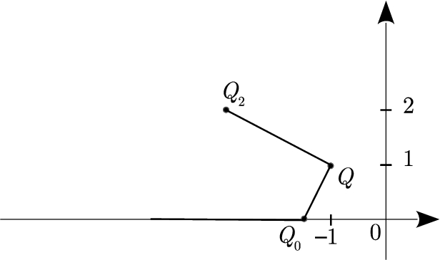
To start, we will consider the following condition: $\begin{matrix} (5) & p_{0} + p_{2} < - 2, p_{1} ⩽ - 1 . \end{matrix}$ In this case, the right boundary of the polygon N consists of the edges $[Q Q_{0}]$ , $[Q Q_{2}]$ and the vertex Q (see Fig. 1).
Fig. 1.
The asymptotic forms of all the continuable solutions of Equation (1) under condition (5) are given in Theorem 1.

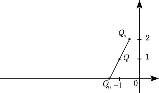
If $\begin{matrix} (6) & p_{0} + p_{2} = - 2, p_{1} ⩽ - 1, \end{matrix}$ then the right boundary of the polygon N is formed by the right edge $[Q_{0} Q_{2}]$ , where the point Q is located (see Fig. 2).
Fig. 2.
In this case, Equation (1) may not have continuable solutions. Theorem 2 uses the truncated equation corresponding to the edge $[Q_{0} Q_{2}]$ to determine the conditions for the existence of continuable solutions. Theorem 3 gives the asymptotic forms of the continuable solutions of Equation (1) in this case.

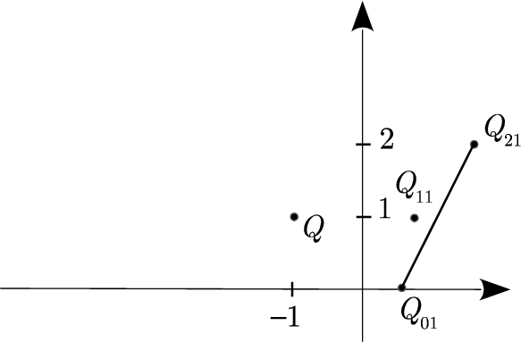
Let us now consider those cases when the point Q does not belong to the right boundary of the polygon N, i.e. when the condition $\begin{matrix} max (p_{0} + p_{2}, 2 p_{1}) > - 2 \end{matrix}$ holds. In this case, (3) is not enough to determine the asymptotic forms of the solutions of Equation (1). For that reason, we will assume that the conditions $\begin{matrix} (7) & \begin{array}{l} f_{i} (x) = \sum_{j = 1}^{L_{i}} c_{i j} x^{p_{i j}} + o (x^{p_{i L_{i}} - ε}), c_{i j}, p_{i j}, ε = const, p_{i j + 1} < p_{i j}, \\ ε > 0, p_{i L_{i}} < - 2 - L, L = | p_{01} | + | p_{11} | + | p_{21} |, \\ i \in {0, 1, 2}, c_{01} c_{11} c_{21} \neq 0, \end{array} \end{matrix}$ are fulfilled.

In Theorem 4, we prove that if (7) and the conditions $\begin{matrix} (8) & p_{11} > - 1, p_{01} + p_{21} < 2 p_{11}, \end{matrix}$ hold (here the right boundary of N consists of the edges $[Q_{11} Q_{01}]$ , $[Q_{11} Q_{21}]$ and the vertex $Q_{11}$ ), then Equation (1) always has continuable solutions. Theorem 4 also provides the asymptotic forms for all such solutions (see Fig. 3).
Fig. 3.
If (7) and the conditions $\begin{matrix} (9) & p_{01} + p_{21} > - 2, p_{01} + p_{21} ⩾ 2 p_{11} \end{matrix}$ hold, then the right boundary of the Newton polygon consists of the edge $[Q_{01} Q_{21}]$ (see Fig. 4).
Fig. 4.
In this case, continuable solutions to Equation (1) need not always exist. The existence of such solutions depends primarily on the existence of such solutions for the truncated equation corresponding to the edge $[Q_{01} Q_{21}]$ . When the inequalities in (9) hold true, the truncated equation is quadratic. Theorem 5 shows that if this equation does not have solutions, then Equation (1) does not have continuable solutions. In Theorem 6, we prove that if the discriminant of the truncated equation is positive, then Equation (1) has continuable solutions. Also, we provide the asymptotic forms of all such solutions. The most difficult case, namely that of a truncated equation with discriminant zero, is considered in Theorem 7. The existence of continuable solutions in this case depends not only on the truncated equation corresponding to the edge $[Q_{01} Q_{21}]$ . We define an iterative process as a result of which we determine the conditions for the existence (or non-existence) of continuable solutions. We also provide the asymptotic forms for the continuable solutions.

In Theorem 8, we apply the previous results to the asymptotical analysis of the solutions of Equation (1) in a neighbourhood of a finite point $x = x_{0}$ . For brevity, we restrict ourselves to the description of the asymptotic forms of such solutions in the case when the functions $f_{i} (x)$ , $i \in {0, 1, 2}$ , satisfy the condition $\begin{matrix} (10) & \begin{matrix} f_{i} (x) = {(x - x_{0})}^{p_{i}} (c_{i} + o ({(x - x_{0})}^{ε})), \\ c_{i}, p_{i}, ε = const, p_{i} ⩾ 0, ε > 0, c_{2} \neq 0, \end{matrix} \end{matrix}$ when $x \to x_{0} + 0$ .
2. The main results

Note 1.
To formulate the results when assuming (5) or (6), it is convenient to rewrite the function $f_{1} (x)$ as $\begin{matrix} f_{1} (x) = x^{- 1} ({\tilde{c}}_{1} + o (x^{- ε})), \end{matrix}$ where ${\tilde{c}}_{1} = c_{1}$ if $p_{1} = - 1$ , and ${\tilde{c}}_{1} = 0$ if $p_{1} < - 1$ .

Furthermore, when assuming (9), we will write the function $f_{1} (x)$ as $\begin{matrix} f_{1} (x) = x^{{\tilde{p}}_{11}} ({\tilde{c}}_{11} + o (x^{- ε})), \end{matrix}$ where ${\tilde{p}}_{11} = 0.5 (p_{01} + p_{21})$ and ${\tilde{c}}_{11} = c_{11}$ if $p_{11} = {\tilde{p}}_{11}$ , and ${\tilde{c}}_{11} = 0$ if $p_{11} < {\tilde{p}}_{11}$ .

We also will use the following notations:

M for the set of continuable solutions;

$M_{i}$ , $M_{j a}$ , $i \in {1, \dots, 10}$ , $j \in {1, 2, 3, 4}$ for the sets of continuable solutions having asymptotic forms given, respectively, by the functions $u_{i} (x)$ and $u_{j a} (x)$ : $\begin{array}{l} u_{1} (x) = \frac{- c_{0}}{p_{0} + {\tilde{c}}_{1} + 1} x^{p_{0} + 1}, u_{2} (x) = \frac{p_{2} - {\tilde{c}}_{1} + 1}{c_{2}} x^{- p_{2} - 1}, \\ u_{3} (x) = \frac{- p_{0} - {\tilde{c}}_{1} - 1 - \sqrt{{(p_{0} + {\tilde{c}}_{1} + 1)}^{2} - 4 c_{0} c_{2}}}{2 c_{2}} x^{p_{0} + 1}, \\ u_{4} (x) = \frac{- p_{0} - {\tilde{c}}_{1} - 1 + \sqrt{{(p_{0} + {\tilde{c}}_{1} + 1)}^{2} - 4 c_{0} c_{2}}}{2 c_{2}} x^{p_{0} + 1}, \\ u_{5} (x) = \frac{- p_{0} - {\tilde{c}}_{1} - 1}{2 c_{2}} x^{p_{0} + 1}, \\ u_{6} = \frac{- c_{01}}{c_{11}} x^{p_{01} - p_{11}}, u_{7} = \frac{- c_{11}}{c_{21}} x^{p_{11} - p_{21}}, \\ u_{8} = \frac{- {\tilde{c}}_{11} - \sqrt{{\tilde{c}}_{11}^{2} - 4 c_{01} c_{21}}}{2 c_{21}} x^{p_{01} - {\tilde{p}}_{11}}, \\ u_{9} = \frac{- {\tilde{c}}_{11} + \sqrt{{\tilde{c}}_{11}^{2} - 4 c_{01} c_{21}}}{2 c_{21}} x^{p_{01} - {\tilde{p}}_{11}}, u_{10} = \frac{- c_{11}}{2 c_{21}} x^{p_{01} - p_{11}}, \\ u_{1 a} (x) = a x^{- {\tilde{c}}_{1}}, where a \neq 0 is an arbitrary constant, \\ u_{2 a} (x) = (a - c_{0} ln x) x^{p_{0} + 1}, where a is an arbitrary constant, \\ u_{3 a} (x) = {(a + c_{2} ln x)}^{- 1} x^{- p_{2} - 1}, where a is an arbitrary constant, \\ u_{4 a} (x) = (\frac{- p_{0} - {\tilde{c}}_{1} - 1}{2 c_{2}} + \frac{1}{a + c_{2} ln x}) x^{p_{0} + 1}, where a is an arbitrary constant . \end{array}$

In the following theorem, we show that if (3) and (5) hold, then the asymptotic forms of the continuable solutions of Equation (1) depend on the relative position of the points $- {\tilde{c}}_{1}$ , $p_{0} + 1$ , $- p_{2} - 1$ on the numerical axis.
Theorem 1.
If ( 3 ) and ( 5 ) hold, then the set M of the continuable solutions of Equation ( 1 ) can be written as a union of the following non-empty sets:
$M = M_{1} \cup M_{2}$ when $- {\tilde{c}}_{1} < p_{0} + 1 < - p_{2} - 1$ , and also when $p_{0} + 1 < - p_{2} - 1 < - {\tilde{c}}_{1}$ ;

$M = M_{1} \cup M_{2} \cup M_{1 a}$ when $p_{0} + 1 < - {\tilde{c}}_{1} < - p_{2} - 1$ ;

$M = M_{2} \cup M_{2 a}$ when $p_{0} + 1 = - {\tilde{c}}_{1} < - p_{2} - 1$ ;

$M = M_{1} \cup M_{3 a}$ when $p_{0} + 1 < - {\tilde{c}}_{1} = - p_{2} - 1$ .

In Theorems 2 and 3, we formulate a criterion for the existence of continuable solutions of Equation (1) when (6) is assumed. Here we also describe the asymptotic forms of such solutions when this criterion holds. We use the notations introduced in Note 1.
Theorem 2.
If ( 3 ) and ( 6 ) hold, then the inequality ${(p_{0} + {\tilde{c}}_{1} + 1)}^{2} - 4 c_{0} c_{2} ⩾ 0$ is a necessary condition for the existence of continuable solutions of Equation ( 1 ).
Theorem 3.
If ( 3 ) and ( 6 ) hold, and moreover, ${(p_{0} + {\tilde{c}}_{1} + 1)}^{2} - 4 c_{0} c_{2} ⩾ 0$ , then the set M of continuable solutions of Equation ( 1 ) is the union of the following non-empty sets: $\begin{array}{l} M = M_{3} \cup M_{4} when {(p_{0} + {\tilde{c}}_{1} + 1)}^{2} - 4 c_{0} c_{2} > 0, \\ M = M_{5} \cup M_{4 a} when {(p_{0} + {\tilde{c}}_{1} + 1)}^{2} - 4 c_{0} c_{2} = 0 . \end{array}$

Below, we consider the cases when the point Q does not belong to the right boundary of the polygon N and (7) holds.
Theorem 4.
If ( 7 ) and ( 8 ) hold, then the set M of continuable solutions of Equation ( 1 ) is a union of two non-empty sets, namely $M = M_{6} \cup M_{7}$ .

We formulate now a necessary condition for the existence of continuable solutions when (9) holds. In this case, it suffices to assume (3) instead of (7). Below, we suppose that ${\tilde{c}}_{1} = c_{1}$ when $p_{0} + p_{2} = 2 p_{1}$ , and ${\tilde{c}}_{1} = 0$ when $p_{0} + p_{2} > 2 p_{1}$ .
Theorem 5.
If ( 3 ) hold, and moreover, $p_{0} + p_{2} ⩾ 2 p_{1}$ , $p_{0} + p_{2} > - 2$ , then Equation ( 1 ) does not have continuable solutions when $4 c_{0} c_{2} - {\tilde{c}}_{1}^{2} > 0$ .

In Theorem 6, we assume that ${\tilde{c}}_{11}$ is defined as in Note 1. Theorem 6.
Assume that ( 7 ) and ( 9 ) hold. If the inequality ${\tilde{c}}_{11}^{2} - 4 c_{01} c_{21} > 0$ is true, then the set M of continuable solutions of Equation ( 1 ) is a union of two non-empty sets, namely $M = M_{8} \cup M_{9}$ .
Theorem 7.
Assume that ( 7 ) holds, and moreover, $p_{01} + p_{21} = 2 p_{11} > - 2$ and $c_{11}^{2} - 4 c_{01} c_{21} = 0$ . If the set M is non-empty, then $M = M_{10}$ .
Note 2.
In the proof of Theorem 7, we define an iterative process that in a finite number of steps makes it possible to determine whether Equation (1) has continuable equations.
Note 3.
We will see from the proofs given in the next section that Theorems 1–5 remain true in the case when $c_{0} c_{2} \neq 0$ , $c_{1} = 0$ , while Theorem 6 is valid in the case when $c_{01} c_{21} \neq 0$ , $c_{11} = 0$ .
Theorem 8.
Assume that ( 10 ) holds. If $y = y (x)$ is a solution of Equation ( 1 ) defined at the point $x_{0}$ and, moreover, $y (x_{0}) \neq 0$ , then there exists a right half neighbourhood of the point $x_{0}$ in which the solution $y (x)$ has the following form: $\begin{matrix} (11) & y (x) = y (x_{0}) + o ({(x - x_{0})}^{δ}), δ = const > 0 . \end{matrix}$ If $y (x_{0}) = 0$ , then there exists a right half neighbourhood of the point $x_{0}$ in which the solution has the form $\begin{matrix} (12) & y (x) = {(x - x_{0})}^{p_{0} + 1} (\frac{- c_{0}}{p_{0} + 1} + o ({(x - x_{0})}^{δ})), δ = const > 0 . \end{matrix}$ There also exist solutions of Equation ( 1 ) not defined at the point $x_{0}$ . In some right half neighbourhood of the point $x_{0}$ , such solutions have the following form: $\begin{matrix} (13) & y (x) = {(x - x_{0})}^{- p_{2} - 1} (\frac{p_{2} + 1}{c_{2}} + o ({(x - x_{0})}^{δ})), δ = const > 0 . \end{matrix}$

3. Proofs of the theorems

In the proofs of Theorems 1–7, we will consider Equation (1) in some neighbourhood $U = {x : x ⩾ S > 1}$ of the point $x = + \infty$ . We will need the following lemmas.

Lemma 1.

Assume that the function $h (x) \in C^{1}$ for $x \in U$ . Let us suppose that there exist some numbers $ε, D > 0$ such that $h (x)$ satisfies one of the following two conditions:

either $\begin{matrix} (14) & | h^{'} (x) x^{1 + ε} | ⩽ D, x ⩾ S, \end{matrix}$

or, for some $S_{1} ⩾ S$ , $\begin{matrix} (15) & | h^{'} (x) x^{1 - ε} | ⩾ D, x ⩾ S_{1} . \end{matrix}$

If ( 14 ) holds, then, for some $S_{2} ⩾ S$ , we obtain the following estimate: $\begin{matrix} (16) & | \int_{b}^{x} e^{h (t)} t^{k} d t | ⩽ \frac{2}{| k + 1 |} e^{h (x)} x^{k + 1}, k = const \neq - 1, x ⩾ S_{2}, \end{matrix}$ where $b = S_{2}$ when $k > - 1$ and $b = + \infty$ when $k < - 1$ .

If ( 15 ) holds, then, for some $S_{2} ⩾ S_{1}$ , we obtain the following estimate: $\begin{matrix} (17) & | \int_{b}^{x} e^{h (t)} t^{k} d t | ⩽ e^{h (x)} x^{k + 1}, k = const, x ⩾ S_{2}, \end{matrix}$ where $b = S_{2}$ when $h^{'} (x) x^{1 - ε} ⩾ D$ and $b = + \infty$ when $h^{'} (x) x^{1 - ε} ⩽ - D$ .

Proof.

We first will prove the estimate (16). Consider the functions $g_{1} (x)$ , $g_{2} (x)$ on the left and right sides of inequality (16). For these functions, we have $\begin{array}{l} g_{1}^{'} (x) = e^{h (x)} x^{k}, k > - 1; g_{1}^{'} (x) = - e^{h (x)} x^{k}, k < - 1; \\ g_{2}^{'} (x) = \frac{2}{| k + 1 |} (k + 1 + x h^{'} (x)) e^{h (x)} x^{k} . \end{array}$ If $k > - 1$ , then $g_{1} (b) = 0$ and $g_{2} (b) > 0$ . We deduce from (14) that the inequality $g_{1}^{'} (x) ⩽ g_{2}^{'} (x)$ holds for sufficiently large $S_{2} ⩾ S$ and $x ⩾ S_{2}$ , and the estimate (16) follows from this. If $k < - 1$ , then, from the definition of the functions $g_{1} (x)$ , $g_{2} (x)$ and (14), we obtain the conditions $\begin{matrix} lim_{x \to + \infty} g_{i} (x) = 0, i = 1, 2, g_{1}^{'} (x) ⩾ g_{2}^{'} (x), x ⩾ S_{2}, \end{matrix}$ for a sufficiently large number $S_{2} ⩾ S$ . We deduce from this the inequality $g_{1} (x) ⩽ g_{2} (x)$ for $x ⩾ S_{2}$ , i.e. the estimate (16) holds for $k < - 1$ .

Assume now that (15) holds true. Define the function $g_{3} (x) = e^{h (x)} x^{k + 1}$ . If $h^{'} (x) x^{1 - ε} ⩾ D$ , then, in a similar manner as above, we get that the inequality $g_{1} (x) ⩽ g_{3} (x)$ is true for sufficiently large $S_{2} ⩾ S$ and $x ⩾ S_{2}$ . Thus, (17) holds for $h^{'} (x) x^{1 - ε} ⩾ D$ .

Assume now that the inequality $h^{'} (x) x^{1 - ε} ⩽ - D$ holds true. Then, it is not difficult to see that the function $g_{1} (x)$ is well-defined, and for sufficiently large $S_{2} ⩾ S$ and $x ⩾ S_{2}$ , we get ${lim}_{x \to + \infty} g_{i} (x) = 0$ , $i = 1, 3$ , $g_{1}^{'} (x) ⩾ g_{3}^{'} (x)$ , $x ⩾ S_{2}$ . We deduce from this the estimate (17) for $h^{'} (x) x^{1 - ε} ⩽ - D$ . This finishes the proof of Lemma 1. □

Consider now an equation of the form (1): $\begin{matrix} (18) & z^{'} + \sum_{i = 0}^{2} g_{i} (x) z^{i} = 0, g_{i} (x) \in C^{0}, x \in U, \end{matrix}$ where $| g_{i} (x) | ⩽ A x^{q_{i}}$ , $i = 0, 2$ , $A, q_{i} = const$ , $A > 0$ , and the function $g_{1} (x)$ satisfies one of the following two conditions when $x \to + \infty$ :

either $\begin{matrix} (19) & g_{1} (x) = x^{q_{1}} (A_{1} + o (x^{- ν})), A_{1}, q_{1}, ν = const, q_{1} > - 1, A_{1} \neq 0, ν > 0, \end{matrix}$

or $\begin{matrix} (20) & g_{1} (x) = x^{- 1} (A_{1} + o (x^{- ν})), A_{1}, ν = const, ν > 0 . \end{matrix}$

Lemma 2.

If $q_{0} + q_{2} < - 2$ , then, for any $δ > 0$ , there exist a number $S_{1} = S_{1} (δ) ⩾ S$ and also a solution $z (x) = z_{δ} (x)$ of Equation ( 18 ) that is defined for $x ⩾ S_{1}$ and satisfies the inequality $\begin{matrix} (21) & | z (x) | ⩽ x^{q_{0} + 1 + δ}, x ⩾ S_{1} . \end{matrix}$

Proof.

Let us write Equation (18) in integral form: $\begin{matrix} (22) & z (x) = e^{- h (x)} \int_{b}^{x} e^{h (t)} G (z (t), t) d t, G (z, t) = - g_{2} (t) z^{2} - g_{0} (t), \end{matrix}$ where, assuming (19), we have $h (x) = \int_{S_{1}}^{x} g_{1} (τ) d τ$ , and either $b = S_{1}$ if $A_{1} > 0$ or $b = + \infty$ if $A_{1} < 0$ , while assuming (20), we have $h (x) = A_{1} ln x + h_{1} (x)$ , $h_{1} (x) = \int_{+ \infty}^{x} (g_{1} (τ) - A_{1} τ^{- 1}) d τ$ , and either $b = S_{1}$ if $A_{1} + q_{0} ⩾ - 1$ or $b = + \infty$ if $A_{1} + q_{0} < - 1$ . The number $S_{1} ⩾ S$ is to be determined later.

Write $γ = - q_{0} - q_{2} - 2 > 0$ and define $μ > 0$ as follows. If (19) holds true, then set $μ = 0.5 γ$ , whereas if (20) is true, then set $μ = 0.5 γ$ when $A_{1} + q_{0} = - 1$ , and $μ = min (0.5 γ, | A_{1} + q_{0} + 1 |)$ when $A_{1} + q_{0} \neq - 1$ .

We will prove the lemma assuming that $0 < δ ⩽ μ$ . It is evident that the lemma for any $δ > 0$ will follow from this.

Consider the following space Ω of functions $z = z (x)$ continuous for $x ⩾ S_{1}$ : $Ω = {z (x) : | z (x) | ⩽ x^{q_{0} + 1 + δ}, x ⩾ S_{1}}$ . Define a mapping H and a norm $‖ z ‖_{1}$ in the space Ω as follows: $\begin{matrix} (23) & H (z (x)) = e^{- h (x)} \int_{b}^{x} e^{h (t)} G (z (t), t) d t, {‖ z (x) ‖}_{1} = sup_{x ⩾ S_{1}} | z (x) x^{- (q_{0} + 1 + δ)} | . \end{matrix}$

We will prove that it is possible to find a number $S_{1} ⩾ S$ such that $H (z) \in Ω$ for $z \in Ω$ and H is a contraction mapping on Ω.

If $z \in Ω$ then $| g_{2} (t) z^{2} (t) | ⩽ A t^{q_{0}}$ . Here we have taken into account that $q_{2} + 2 (q_{0} + 1 + δ) = q_{0} - γ + 2 δ ⩽ q_{0}$ . From the estimate obtained, we deduce that $| G (z (t), t) | ⩽ 2 A t^{q_{0}}$ for $z (t) \in Ω$ .

Assume that (19) holds. Then, by Lemma 1, it follows that the estimate $| H (z (x)) | ⩽ x^{q_{0} + 1 + δ}$ holds if $z (x) \in Ω$ and $S_{1}^{δ} ⩾ 2 A$ for $x ⩾ S_{1}$ , which means that $H (z (x)) \in Ω$ . Assume now that $z_{i} (x) \in Ω$ , $i = 1, 2$ , $‖ z_{1} - z_{2} ‖_{1} = ρ$ , $ρ = const > 0$ . Then $| g_{2} (t) (z_{1}^{2} (t) - z_{2}^{2} (t)) | ⩽ 2 A ρ t^{q_{2} + 2 q_{0} + 2 + 2 δ} ⩽ 2 A ρ t^{q_{0}}$ . From this, we come to the conclusion that the estimate $\begin{matrix} | H (z_{1} (x)) - H (z_{2} (x)) | ⩽ 2 A ρ x^{q_{0} + 1} ⩽ 0.5 ρ x^{q_{0} + 1 + δ} \end{matrix}$ is true for $x ⩾ S_{1}$ and $S_{1}^{δ} ⩾ 4 A$ , i.e. $‖ H (z_{1}) - H (z_{2}) ‖_{1} ⩽ 0.5 ρ$ .

Assuming (20) in place of (19), we get $\begin{matrix} H (z (x)) = x^{- A_{1}} e^{- h_{1} (x)} \int_{b}^{x} e^{h_{1} (t)} t^{A_{1}} G (z (t), t) d t, \end{matrix}$ and if $z (x) \in Ω$ , we arrive at the estimate $| t^{A_{1}} G (z (t), t) | ⩽ 2 A t^{A_{1} + q_{0}} ⩽ 2 A t^{A_{2}}$ , $A_{2} = A_{1} + q_{0} + 0.5 δ$ , and moreover, by the definition of δ, we get $| A_{2} + 1 | ⩾ 0.5 δ$ . By Lemma 1, it follows that the estimate $| H (z (x)) | ⩽ 4 A δ^{- 1} x^{q_{0} + 1 + 0.5 δ} ⩽ x^{q_{0} + 1 + δ}$ is true if $z (x) \in Ω$ and $S_{1}^{0.5 δ} ⩾ 4 A δ^{- 1}$ , which means that $H (z (x)) \in Ω$ . By a similar argument as above, we conclude that the estimate $\begin{matrix} | H (z_{1} (x)) - H (z_{2} (x)) | ⩽ 2 A δ^{- 1} ρ x^{q_{0} + 1 + 0.5 δ} ⩽ 0.5 ρ x^{q_{0} + 1 + δ}, \end{matrix}$ holds if $z_{i} (x) \in Ω$ , $i = 1, 2$ , $‖ z_{1} - z_{2} ‖_{1} = ρ$ , $ρ = const > 0$ for $x ⩾ S_{1}$ , $S_{1}^{0.5 δ} ⩾ 4 A δ^{- 1}$ , said otherwise, $‖ H (z_{1}) - H (z_{2}) ‖_{1} ⩽ 0.5 ρ$ . We have thus proven that H is a contraction mapping on Ω.

Taking into account now that Ω is a complete space, it follows from the above that the mapping H has a fixed point in Ω. Equation (18) has therefore a solution $z (x)$ satisfying the estimate (21) for $x ⩾ S_{1}$ . This concludes the proof of Lemma 2. □

The proof of the results related to the structure of the asymptotic forms for the solutions of Equation (1) is based on the following scheme. If we know two continuable solutions of the equation, then it is not difficult to obtain the general solution by means of a single quadrature. Indeed, assume that $y_{1} (x) \neq y_{2} (x)$ are both particular solutions to Equation (1). If we make the substitution $y = y_{1} (x) + w$ , we obtain the homogeneous equation $\begin{matrix} (24) & w^{'} + w^{2} f_{2} (x) + w (2 f_{2} (x) y_{1} (x) + f_{1} (x)) = 0 . \end{matrix}$ To find nontrivial solutions to this equation, make the substitution $w = z^{- 1}$ . Then Equation (24) transforms into $\begin{matrix} (25) & z^{'} - z (2 f_{2} (x) y_{1} (x) + f_{1} (x)) - f_{2} (x) = 0 . \end{matrix}$

The function $z_{1} (x) = {(y_{2} (x) - y_{1} (x))}^{- 1}$ is a solution of Equation (25). By means of the substitution $z = z_{1} (x) + v$ , this equation becomes $\begin{matrix} (26) & v^{'} - v (2 f_{2} (x) y_{1} (x) + f_{1} (x)) = 0 . \end{matrix}$

The family of functions $v = C e^{g (x)}$ , where C is an arbitrary constant and $g (x)$ is one of the primitives of the function $2 f_{2} (x) y_{1} (x) + f_{1} (x)$ , is the general solution of Equation (26). It follows from this that the general solution of Equation (1) has either the form

$y = y_{1} (x)$ or the form $\begin{matrix} (27) & y = y_{1} (x) + {({(y_{2} (x) - y_{1} (x))}^{- 1} + C e^{g (x)})}^{- 1}, \end{matrix}$ where C is an arbitrary constant. If we know three different solutions of Equation (1), then the general solution can be obtained without need of quadrature. Indeed, if, in addition to $y_{1} (x)$ and $y_{2} (x)$ , we have a third solution $y_{3} (x)$ , then by substituting it into (27), we obtain $\begin{matrix} C_{1} e^{g (x)} = {(y_{3} (x) - y_{1} (x))}^{- 1} - {(y_{2} (x) - y_{1} (x))}^{- 1}, C_{1} = const . \end{matrix}$

From this and (27), it is easily seen that the general solution of Equation (1) has either the form

$y = y_{1} (x)$ or the form $\begin{matrix} (28) & y = y_{1} (x) + \frac{(y_{2} (x) - y_{1} (x)) (y_{3} (x) - y_{1} (x))}{y_{3} (x) - y_{1} (x) + C (y_{2} (x) - y_{3} (x))}, \end{matrix}$ where C is an arbitrary constant.

Proof of Theorem 1.

We begin by considering Cases 1 and 2. We shall show that Equation (1) has a solution $y_{1} (x)$ having an asymptotic form given by the function $u_{1} (x)$ . If $- {\tilde{c}}_{1} \neq p_{0} + 1$ , then the function $u = u_{1} (x)$ is a solution of the truncated equation $u^{'} + {\tilde{c}}_{1} x^{- 1} u + c_{0} x^{p_{0}} = 0$ which corresponds to the edge $[Q_{0} Q]$ of the Newton polygon N of Equation (4). By means of the substitution $y = z + u_{1} (x)$ into Equation (1), we get an equation of the form (18), where $\begin{array}{l} g_{0} (x) = f_{0} (x) - c_{0} x^{p_{0}} + u_{1}^{2} (x) f_{2} (x) + u_{1} (x) (f_{1} (x) - {\tilde{c}}_{1} x^{- 1}), \\ g_{1} (x) = f_{1} (x) + 2 f_{2} (x) u_{1} (x), g_{2} (x) = f_{2} (x), | g_{i} (x) | ⩽ D x^{q_{i}}, \\ D = const > 0, q_{i} = const, i \in {0, 1, 2}, q_{0} < p_{0}, q_{0} + q_{2} < - 2, q_{1} = - 1 . \end{array}$ Here the conditions of Lemma 2 hold true, and therefore the equation obtained has a solution $z = z_{1} (x)$ that satisfies the estimate (21), namely $| z_{1} (x) | ⩽ x^{r}$ , $r = q_{0} + 1 + δ$ , whence, assuming that $0 < δ < p_{0} - q_{0}$ , we obtain $r < p_{0} + 1$ . From here it follows that the function $u_{1} (x)$ is an asymptotic form for the solution $y_{1} (x) = z_{1} (x) + u_{1} (x)$ .

By means of the substitution $y = w^{- 1}$ , we transform Equation (1) into $w^{'} - f_{0} (x) w^{2} - f_{1} (x) w - f_{2} (x) = 0$ . Similarly as above, but assuming that ${\tilde{c}}_{1} \neq p_{2} + 1$ , we conclude that the equation we have obtained has a solution $w = w_{1} (x)$ with an asymptotic form given by the function $c_{2} {(p_{2} - {\tilde{c}}_{1} + 1)}^{- 1} x^{p_{2} + 1} = {(u_{2} (x))}^{- 1}$ . It follows from this fact that Equation (1) has a solution $y_{2} (x)$ with an asymptotic form given by the function $u_{2} (x)$ .

The function $u_{1 a} (x) = a x^{- {\tilde{c}}_{1}}$ , $a = const \neq 0$ , is a nontrivial solution of the truncated equation $u^{'} + {\tilde{c}}_{1} x^{- 1} u = 0$ , which corresponds to the vertex Q of the polygon N. By means of the substitution $y = z + u_{1 a} (x)$ in (1), we obtain an equation of the form (18), in which $\begin{array}{l} g_{0} (x) = f_{0} (x) + u_{1 a}^{2} (x) f_{2} (x) + u_{1 a} (x) (f_{1} (x) - {\tilde{c}}_{1} x^{- 1}), \\ g_{1} (x) = f_{1} (x) + 2 u_{1 a} (x) f_{2} (x), g_{2} (x) = f_{2} (x), | g_{i} (x) | ⩽ D x^{q_{i}}, \\ D = const > 0, q_{i} = const, i \in {0, 1, 2} . \end{array}$

If one assumes that $p_{0} + 1 < - {\tilde{c}}_{1} < - p_{2} - 1$ (Case 2), then the conditions $q_{0} < - {\tilde{c}}_{1} - 1$ , $q_{0} + q_{2} < - 2$ and $q_{1} = - 1$ hold. Consequently, the conditions of Lemma 2 hold, and therefore the equation obtained has a solution $\tilde{z} (x)$ that satisfies the estimate (21), i.e. $| \tilde{z} (x) | ⩽ x^{r}$ , $r = q_{0} + 1 + δ$ , where, assuming that $0 < δ < - {\tilde{c}}_{1} - q_{0} - 1$ , it follows that $r < - {\tilde{c}}_{1}$ . It may be concluded from this that the function $u_{1 a} (x)$ is an asymptotic form of the solution $y_{3} (x) = \tilde{z} (x) + u_{1 a} (x)$ .

Note that the function $x^{{\tilde{c}}_{1}}$ is an asymptotic form of the function $e^{g (x)}$ with $\begin{matrix} g (x) = {\tilde{c}}_{1} ln x + \int_{+ \infty}^{x} (2 f_{2} (t) y_{1} (t) + f_{1} (t) - {\tilde{c}}_{1} t^{- 1}) d t . \end{matrix}$

Assume that $C \neq 0$ in (27). If the inequality $- {\tilde{c}}_{1} > - p_{2} - 1$ holds, then the function $u_{2} (x)$ is an asymptotic form of the solution $y (x)$ , whereas if $- {\tilde{c}}_{1} < p_{0} + 1$ , then the function $u_{1} (x)$ is an asymptotic form of the solution $y (x)$ . If we assume that $p_{0} + 1 < - {\tilde{c}}_{1} < - p_{2} - 1$ , then, from (28) with $C \neq 0$ , it follows that the function $u_{1 a} (x)$ is an asymptotic form of the solution $y (x)$ . In addition, Equation (1) in Cases 1 and 2 has solutions $y_{1} (x)$ and $y_{2} (x)$ with asymptotic forms $u_{1} (x)$ and $u_{2} (x)$ , respectively. This completes the proof of Theorem 1 in Cases 1 and 2.

In Case 3, we prove as above that there exist solutions $y_{i} (x)$ , $i = 1, 2$ , with asymptotic forms given by the functions $u_{2 a} (x)$ and $u_{2} (x)$ , respectively. By substituting $y_{i} = y_{i} (x)$ , $i = 1, 2$ , into (27), we show that if $C = 0$ then $y (x) \in M_{2}$ , and if $C \neq 0$ then $y (x) \in M_{2 a}$ . The proof for Case 4 is similar. The proof of Theorem 1 is complete. □

Proof of Theorem 2.

Let us make in (1) the substitution $\begin{matrix} y = \frac{2 w + p_{2} - {\tilde{c}}_{1} x^{p_{1} + 1}}{2 c_{2} x^{p_{2} + 1}} . \end{matrix}$ Now, taking into account the conditions of the theorem, we see that Equation (1) takes the form $\begin{array}{l} x w^{'} + w^{2} (1 + o (x^{- α})) - w (1 + o (x^{- α})) + a (x) = 0, a (x) = A + o (x^{- α}), \\ A, α = const, α > 0, A > 0.25, \end{array}$ in a neighbourhood of the point $x = + \infty$ .

It is easily shown that if $w (x)$ is a continuable solution of the equation, then the function $| w (x) |$ is bounded in a neighbourhood of the point $x = + \infty$ . But this means that there exists a neighbourhood of the point $x = + \infty$ in which the inequality $\begin{matrix} x w^{'} + w^{2} - w + A_{1} < 0, A_{1} = const > 0.25, \end{matrix}$ is true.

By integration of the previous inequality, we prove that the function $w (x)$ cannot be defined in a neighbourhood of the point $x = + \infty$ , that is, all of the solutions of Equation (1) are not continuable. This proves Theorem 2. □

Proof of Theorem 3.

To begin, assume that $d = {(p_{0} + {\tilde{c}}_{1} + 1)}^{2} - 4 c_{0} c_{2} > 0$ . The proof in this case is almost the same as in Case 1 of Theorem 1. Firstly, we show that Equation (1) has two solutions $y_{1} (x)$ and $y_{2} (x)$ having asymptotic forms given by the functions $u_{3} (x)$ and $u_{4} (x)$ , respectively. Here, the asymptotic form of the function $e^{g (x)}$ in (27) is the function $x^{- (p_{0} + 1 + d)}$ . By substituting these functions into (27), we ascertain that all of the solutions of Equation (1) in the case we are considering belong to either $M_{3}$ or $M_{4}$ . If we assume that $d = 0$ , then, by a similar argument as above, we can show that Equation (1) has solutions $y_{1} (x)$ and $y_{2} (x)$ with asymptotic forms given, respectively, by the functions $u_{5} (x)$ and $\tilde{u} (x) = u_{4 a} (x)$ for $a = 0$ . In this case, the asymptotic form of the function $e^{g (x)}$ is given by the function $x^{- p_{0} - 1}$ . Now, taking this into account, we deduce from (27) that each solution of Equation (1) belongs to either $M_{5}$ or $M_{4 a}$ . This finishes the proof of Theorem 3. □

Proof of Theorem 4.

We will show that Equation (1) has a solution with an asymptotic form given by the function $u_{6} (x) = a_{1} x^{s_{1}}$ , $s_{1} = p_{01} - p_{11}$ , $a_{1} = - c_{01} {(c_{11})}^{- 1}$ . In correspondence with (7), let us write $\begin{matrix} f_{i} (x) = f_{i}^{*} (x) + {\tilde{f}}_{i} (x), f_{i}^{*} (x) = \sum_{j = 1}^{L_{i}} c_{i j} x^{p_{i j}}, {\tilde{f}}_{i} (x) = o (x^{- 2 - L - ε}), \end{matrix}$ in Equation (1).

By substituting $\begin{matrix} (29) & \begin{matrix} y = w_{k} + h_{k} (x), h_{k} (x) = \sum_{j = 1}^{k} v_{j} (x), k = 1, 2, \dots, \\ v_{j} (x) = - f_{0 j - 1}^{*} (x) {(c_{11} x^{p_{11}})}^{- 1}, \\ f_{0 j}^{*} (x) = (v_{j}^{2} (x) + 2 h_{j - 1} (x) v_{j} (x)) f_{2}^{*} (x) + v_{j} (x) f_{11}^{*} (x) + v_{j}^{'} (x), \\ h_{0} (x) = 0, f_{00}^{*} (x) = f_{0}^{*} (x), f_{11}^{*} (x) = f_{1}^{*} (x) - c_{11} x^{p_{11}}, \end{matrix} \end{matrix}$ into Equation (1), we obtain the equations $\begin{matrix} (30) & \begin{matrix} w_{k}^{'} + f_{2} (x) w_{k}^{2} + (f_{1} (x) + 2 h_{k} (x) f_{2} (x)) w_{k} + f_{0 k} (x) = 0, \\ f_{0 k} (x) = f_{0 k}^{*} (x) + {\tilde{f}}_{0 k} (x), {\tilde{f}}_{0 k} (x) = h_{k}^{2} (x) {\tilde{f}}_{2} (x) + h_{k} (x) {\tilde{f}}_{1} (x) + {\tilde{f}}_{0} (x), \end{matrix} \end{matrix}$ which have the same form as Equation (1).

Below, when proving that a function is bounded by a constant regardless which one, we will use the so-called “universal” constant $D > 0$ , for which $D + D = D$ and $D \cdot D = D$ . From (29) and (30), we deduce the estimates $\begin{array}{l} | f_{0 k}^{*} (x) | ⩽ D x^{p_{01} - k β}, | {\tilde{f}}_{0 k} (x) | ⩽ D x^{- 2 - L - ε} (x^{2 s_{1}} + x^{s_{1}} + 1), \\ β = min (2 p_{11} - p_{01} - p_{21}, p_{11} - p_{12}, p_{11} + 1) > 0, x ⩾ S . \end{array}$ This means that for a sufficiently large $k = K$ the estimate $\begin{matrix} | f_{0 K} (x) | ⩽ D x^{q_{0}}, q_{0} = const, q_{0} < - 2 - p_{21} - ε, q_{0} < s_{1} - 1 - ε \end{matrix}$ is valid and, consequently, Equation (30) takes the form (18) with $g_{0} (x) = f_{0 K} (x)$ , $g_{1} (x) = f_{1} (x) + 2 h_{K} (x) f_{2} (x)$ , $g_{2} (x) = f_{2} (x)$ .

Thus the equation obtained satisfies the conditions of Lemma 2. It therefore has a solution $w_{K} (x) = u (x)$ that satisfies the estimate (21), and from this, taking $0 < δ < 0.5 ε$ , we get $| u (x) | ⩽ x^{s_{1} - 0.5 ε}$ . Notice also that the function $a_{1} x^{s_{1}}$ provides an asymptotic form for the function $h_{K} (x)$ . Consequently, the solution $y (x) = y_{1} (x) = u (x) + h_{K} (x)$ of Equation (1) has an asymptotic form given by the function $u_{6} (x)$ . Note that if $a_{1} = 0$ , then the arguments we have provided here imply that Equation (1) has a solution $y (x) = u (x)$ , $| u (x) | ⩽ x^{s_{1} - 0.5 ε}$ .

The substitution $y = w^{- 1}$ changes Equation (1) into $w^{'} - f_{0} (x) w^{2} - f_{1} (x) w - f_{2} (x) = 0$ . According to what we have already proved, the equation obtained has a solution $w_{1} (x)$ with an asymptotic form given by the function $- c_{21} {(c_{11})}^{- 1} x^{p_{21} - p_{11}}$ . It follows that equation (1) has a solution $y_{2} (x)$ having an asymptotic form given by the function $u_{7} (x)$ .

By substituting the functions $y_{1} (x)$ and $y_{2} (x)$ into (27) and observing that $c_{11} x^{p_{11}}$ is an asymptotic form of the function $2 f_{2} (x) y_{1} (x) + f_{1} (x)$ , we see that Theorem 4 follows immediately from (27), thereby completing the proof. □

Proof of Theorem 5.

Make the substitution $\begin{matrix} y = \frac{2 w - {\tilde{c}}_{1} x^{{\tilde{p}}_{1} + 1}}{2 c_{2} x^{p_{2} + 1}}, {\tilde{p}}_{1} = 0.5 (p_{0} + p_{2}), \end{matrix}$ in Equation (1). Now, taking into account the conditions of the theorem, we ascertain that Equation (1) has the form $\begin{array}{l} x w^{'} + w^{2} (1 + o (x^{- α})) + w o (x^{{\tilde{p}}_{1} + 1 - α}) \\ + A_{1} x^{2 ({\tilde{p}}_{1} + 1)} (1 + o (x^{- α})) + A_{2} x^{{\tilde{p}}_{1} + 1} = 0, \\ A_{1}, A_{2}, α = const, A_{1}, α > 0, \end{array}$ in some neighbourhood of the point $x = + \infty$ . There is therefore a neighbourhood of the point $x = + \infty$ where the inequality $\begin{matrix} x w^{'} + A (w^{2} + x^{2 ({\tilde{p}}_{1} + 1)}) < 0, A = const > 0, \end{matrix}$ is true. This inequality implies that $\begin{matrix} x w^{'} + A x^{2 ({\tilde{p}}_{1} + 1)} < 0, x w^{'} + A w^{2} < 0 . \end{matrix}$ From the first inequality, it follows that $w (x) \to - \infty$ when $x \to + \infty$ . With this in mind, by integrating the second inequality, we see that the function $w (x)$ cannot be defined in a neighbourhood of $x = + \infty$ . In consequence, all the solutions of Equation (1) are not continuable. This finishes the proof of Theorem 5. □

Proof of Theorem 6.

Here we follow the notations introduced in Note 1, namely $f_{1} (x) = {\tilde{c}}_{11} x^{{\tilde{p}}_{11}} + \dots$ , where ${\tilde{p}}_{11} = 0.5 (p_{01} + p_{21})$ , and ${\tilde{c}}_{11} = c_{11}$ if $p_{11} = {\tilde{p}}_{11}$ and ${\tilde{c}}_{11} = 0$ if $p_{11} < {\tilde{p}}_{11}$ .

Make in Equation (1) the substitution $y = z + u (x)$ with $\begin{matrix} (31) & u (x) = {(2 c_{21})}^{- 1} (- {\tilde{c}}_{11} - b) x^{p_{01} - {\tilde{p}}_{11}}, b = \sqrt{{\tilde{c}}_{11}^{2} - 4 c_{01} c_{21}} . \end{matrix}$ Note that $- {\tilde{c}}_{11} - b \neq 0$ since $c_{01} c_{21} \neq 0$ . As a result, we obtain an equation of the form (1): $\begin{matrix} (32) & \begin{array}{l} z^{'} + f_{2} (x) z^{2} + f_{11} (x) z + f_{01} (x) = 0, \\ f_{01} (x) = f_{0} (x) - c_{01} x^{p_{01}} + u^{2} (x) (f_{2} (x) - c_{21} x^{p_{21}}) + u (x) (f_{1} (x) - {\tilde{c}}_{11} x^{{\tilde{p}}_{11}}) + u^{'} (x), \\ f_{11} (x) = f_{1} (x) + 2 u (x) f_{2} (x) . \end{array} \end{matrix}$

We will apply to this equation the arguments from the proof of Theorem 4, taking into account that $f_{01} (x) = o (x^{p_{01} - η})$ , $η = const > 0$ , and also that the function $f_{11} (x)$ has an asymptotic form given by the function $- b x^{{\tilde{p}}_{11}}$ . As a result, we deduce that either the solutions of Equation (32) satisfy the condition $z (x) = o (x^{p_{01} - {\tilde{p}}_{11} - η})$ or they have an asymptotic form given by the function $v_{1} (x) = b c_{21}^{- 1} x^{{\tilde{p}}_{11} - p_{21}}$ . Consequently, each solution of Equation (1) has an asymptotic form given either by the function $u (x)$ or by the function $v_{2} (x) = v_{1} (x) + u (x) = {(2 c_{21})}^{- 1} (- {\tilde{c}}_{11} + b) x^{{\tilde{p}}_{11} - p_{21}}$ . This completes the proof of Theorem 6. □

Proof of Theorem 7.

We say that the numbers $p_{i 1}$ , $c_{i 1}$ , $i \in {0, 1, 2}$ , are the determining parameters (or, simply, the parameters) of the equations of the form (1) we will consider further on. The parameters that satisfy the conditions of Theorem 2 or 5 are called inadmissible, otherwise, they are called admissible. For brevity, if Equation (1) satisfies the conditions of Theorem 7, then we say that it is degenerated. Fix the numbers $α = p_{21} - p_{22} > 0$ and $γ = p_{01} - p_{11} = p_{11} - p_{21}$ . The transforms of the form (31) are said to be standard. Consider a sequence of standard transforms that leave Equation (1) degenerated. Note that there is only a finite number of such transforms. Indeed, if a transformed equation is degenerated, then fix a number $k ⩾ 1$ such that $p_{1 k + 1} ⩽ p_{11} - α$ and $p_{1 k} > p_{11} - α$ . It is evident that by means of no more than k standard transforms we can obtain an equation of the form (1), $\begin{matrix} (33) & {\tilde{y}}^{'} + \sum_{i = 0}^{2} {\tilde{f}}_{i} (x) {\tilde{y}}^{i} = 0, \end{matrix}$ with ${\tilde{f}}_{i} (x) = {\tilde{c}}_{i 1} x^{{\tilde{p}}_{i 1}} + \dots$ , $i = 0, 1$ , ${\tilde{f}}_{2} (x) = f_{2} (x)$ , and ${\tilde{p}}_{01} ⩽ p_{01} - α$ , ${\tilde{p}}_{11} ⩽ p_{11} - α$ , ${\tilde{p}}_{21} = p_{21}$ . It is clear that the condition ${\tilde{p}}_{01} + p_{21} > - 2$ is violated after a finite number of transforms that leave Equation (1) degenerated.

If Equation (33) is not degenerated, then the functions ${\tilde{f}}_{0} (x)$ and ${\tilde{f}}_{1} (x)$ satisfy one of the following conditions (below, we use a “universal” constant $D > 0$ ):

$2 {\tilde{p}}_{11} > {\tilde{p}}_{01} + p_{21}$ , ${\tilde{p}}_{11} > - 1$ , ${\tilde{c}}_{01} {\tilde{c}}_{11} \neq 0$ ;

$2 {\tilde{p}}_{11} > {\tilde{p}}_{01} + p_{21}$ , ${\tilde{p}}_{01} + p_{21} > - 2$ , ${\tilde{c}}_{01} \neq 0$ ;

${\tilde{p}}_{01} + p_{21} ⩽ - 2$ , ${\tilde{p}}_{11} ⩽ - 1$ , ${\tilde{c}}_{01} \neq 0$ ;

$| {\tilde{f}}_{0} (x) | ⩽ D x^{q_{0}}$ , $q_{0} < - 2 - p_{21}$ , ${\tilde{p}}_{11} > - 1$ , ${\tilde{c}}_{11} \neq 0$ ;

$| {\tilde{f}}_{0} (x) | ⩽ D x^{q_{0}}$ , $q_{0} < - 2 - p_{21}$ , ${\tilde{p}}_{11} ⩽ - 1$ .

In the first case, it follows from Theorem 4 that the power orders of the asymptotic forms of the continuable solutions are the numbers $γ_{1} = {\tilde{p}}_{01} - {\tilde{p}}_{11}$ and $γ_{2} = {\tilde{p}}_{11} - p_{21}$ , and moreover, $γ_{1} = {\tilde{p}}_{01} - {\tilde{p}}_{11} < {\tilde{p}}_{01} - 0.5 ({\tilde{p}}_{01} + p_{21}) = 0.5 ({\tilde{p}}_{01} - p_{21}) < γ$ and $γ_{2} = {\tilde{p}}_{11} - p_{21} < γ$ .

In the second case, if the parameters of Equation (33) are inadmissible, then this equation has no continuable solutions, and consequently nor does Equation (1). On the contrary, if the parameters are admissible, then it follows from Theorem 4 that the order of the asymptotic forms of the continuable solutions of Equation (33) is the number $γ_{3} = 0.5 ({\tilde{p}}_{01} - p_{21}) < γ$ . The assertion of Theorem 7 in the case considered follows immediately from this.

In the third case, if the parameters of the transformed equation are inadmissible, then the equation has no continuable solutions, and hence neither does Equation (1). On the contrary, if the parameters indicated are admissible, then it follows from Theorem 1 that any continuable solution $\tilde{y} (x)$ satisfies the inequality $| \tilde{y} (x) | ⩽ D x^{- p_{21} - 1}$ , but $- p_{21} - 1 < γ$ , from which the assertion of Theorem 7 in this case follows readily.

In the fourth case, it follows by Lemma 2 and from the arguments given in Theorem 4 that Equation (33) has two continuable solutions $y_{1} (x)$ and $y_{2} (x)$ such that $\begin{array}{l} | y_{1} (x) | ⩽ D x^{r}, r < - p_{21} - 1 < {\tilde{p}}_{11} - p_{21}, \\ y_{2} (x) = B x^{{\tilde{p}}_{11} - p_{21}} (1 + o (x^{- \tilde{ε}})), B, \tilde{ε}, r = const, B \neq 0, \tilde{ε} > 0 . \end{array}$ Now it follows from (27) that any continuable solution $\tilde{y} (x)$ satisfies the inequality $| \tilde{y} (x) | ⩽ D x^{γ_{4}}$ , $γ_{4} ⩽ {\tilde{p}}_{11} - p_{21} < γ$ . The assertion of Theorem 7 in this case is an immediate consequence.

In the fifth case, it follows by Lemma 2 and the arguments given in Theorem 1 that there exist two continuable solutions $y_{1} (x)$ and $y_{2} (x)$ such that $\begin{array}{l} | y_{1} (x) | ⩽ D x^{r}, r < - p_{21} - 1, \\ y_{2} (x) = B x^{- p_{21} - 1} (1 + o (x^{- \tilde{ε}})), B, \tilde{ε}, r = const, B \neq 0, \tilde{ε} > 0 . \end{array}$ In this case, we deduce from (27) that any continuable solution $\tilde{y} (x)$ satisfies the inequality $| \tilde{y} (x) | ⩽ D x^{- p_{21} - 1}$ , and taking into account that $- p_{21} - 1 < γ$ , we conclude that Theorem 7 holds in this case. This completes the proof of Theorem 7. □

Proof of Theorem 8.

Let us make the substitution $t = {(x - x_{0})}^{- 1}$ in Equation (1). Taking into account (10), we obtain the equation $\begin{matrix} (34) & \frac{d y}{d t} - \sum_{i = 0}^{2} {\tilde{f}}_{i} (t) y^{i} = 0, {\tilde{f}}_{i} (t) = t^{- p_{i} - 2} (c_{i} + o (t^{- ε})) . \end{matrix}$ This equation satisfies (5) and has the form (3), with only one difference, namely that $c_{0} = 0$ is possible in (34). It follows from the proof of Theorem 1 (Case 2) that there is a neighbourhood of the point $t = + \infty$ in which Equation (34) has solutions $y_{i} (t)$ , $i \in {1, 2, 3}$ , $y_{1} (t) = t^{- p_{0} - 1} (\frac{- c_{0}}{p_{0} + 1} + o (t^{- δ}))$ , where $δ = const > 0$ , and the functions $y_{2} (t)$ and $y_{3} (t)$ have asymptotic forms given, respectively, by the functions $u_{2} = \frac{p_{2} + 1}{c_{2}} t^{p_{2} + 1}$ and $u_{3} = a$ , where $a \neq 0$ is an arbitrary constant. As we can notice by substituting $y_{i} (t)$ , $i \in {1, 2, 3}$ , into (28), the continuable solutions of Equation (34) belong to one of the following non-empty sets:

solutions of the form $y (t) = t^{- p_{0} - 1} (\frac{- c_{0}}{p_{0} + 1} + o (t^{- δ}))$ ;

solutions of the form $y (t) = t^{p_{2} + 1} (\frac{p_{2} + 1}{c_{2}} + o (t^{- δ}))$ ;

solutions of the form $y (t) = a + o (t^{- δ})$ , $a \neq 0$ is an arbitrary constant.

In the first case, we obtain solutions of the form (12); in the second case, solutions of the form (13), and in the third case, solutions of the form (11). This finishes the proof of Theorem 8. □

References

A.D.

Bruno, Russ. Math. Surv. 59(3) (2004), 429–480. doi:10.1070/RM2004v059n03ABEH000736.

Kamke, Gewohnliche Differentialgleichungen. Leippzig, 1959.

Riccati, Acta Eruditorum (1724), 66–73.

V.S.

Samovol, Doklady Mathematics 96(1) (2017), 373–376. doi:10.1134/S106456241704024X.

V.S.

Samovol, Doklady Mathematics 97(3) (2018), 250–253. doi:10.1134/S106456241803016X.

G.N.

Watson, A Treatise on the Theory of Bessel Functions, Cambridge, 1995. doi:10.2307/3605513.