On decomposition of the fundamental solution of the Helmholtz equation over solutions of iterative parabolic equations

Abstract

Recently, it was shown that the solution of the Helmholtz equation can be approximated by a series over the solutions of iterative parabolic equations (IPEs). An expansion of the fundamental solution of the Helmholtz equation over solutions of IPEs is considered. It is shown that the resulting Taylor-like series can be easily transformed into a Padé-type approximation. In practical propagation problems such iterative Padé approximations exhibit improved wide-angle capabilities and faster convergence to the solution of the Helmholtz equation in comparison to Taylor-like expansion over IPEs solutions. A Gaussian smoothing of the expansion terms gives insight into the derivation of initial conditions consistent for IPEs, which can be used for point source simulation. A correct point source model consistent with the wide-angle one-way propagation equations is important in many practical applications of the parabolic equations theory.

Keywords

Helmholtz equation paraxial approximation multiple scales iterative parabolic equations wide-angle parabolic equations self-starter pattern solver tool

1. Introduction

The method of parabolic equations is currently one of the most important tools for simulating wave propagation in various media [5,6]. In pioneering works wide-angle parabolic equations (PEs) are usually derived using Padé approximations of an operator square root arising from the formal factorization of the Helmholtz operator [1,12]. The solution of such equations allows to simulate one-way wave propagation both efficiently and accurately [5]. It is well known that both the aperture of a PE (i.e., its ability to handle wide-angle effects) and the stability of its solution depend strongly on the choice of the Cauchy data in the particular initial boundary value problem [2,5,10] (often referred to as the starter in PE theory). Various techniques for designing starters have been used in the literature, including analytical methods, normal mode theory, ray theory, and the so-called self-starter approach [2,5,10].

Recently, Trofimov [15] proposed a new approach to the PE theory. Trofimov’s derivation is based on the method of multiple scales [15], and it leads to a system of so-called iterative parabolic equations (IPEs), where the solution of the j-th equation is used to compute the input term of the $j + 1$ -th equation (thus higher order equations can be viewed as a correction to lower order equations). This approach was further developed in [9], and in [11] it was also shown that it can be extended to the case of nonlinear media (leading to first wide-angle parabolic approximations of a nonlinear equation).

This study continues the development of IPE theory. We begin by deriving IPE solutions corresponding to the fundamental solution of the Helmholtz equation. To our knowledge, this correspondence has not been investigated in the literature until now, and the expansion of the fundamental solution of the Helmholtz equation over solutions of parabolic equations can be of interest per se.

Next, we investigate how the Taylor-like series over solutions of IPEs can be transformed into an iterative Padé approximation of this fundamental solution. It is well-known that in the standard wide-angle PE theory based on the operator square root expansions in one-way propagation equations the use of the Padé approximations results in more adequate behaviour of the solutions of resulting PEs and better wide-angle capabilities [5]. In this work we demonstrate that similar conclusion can be also drawn for IPEs. It is shown that iterative Padé approximations exhibit better wide-angle capabilities than the respective Taylor-like series over IPEs solutions (the form in which it was introduced in [15]). It is important to stress that in practice an iterative Padé approximation can be obtained by a simple rearrangement of IPEs solutions, and therefore it requires almost no additional computational effort.

The derivation also shows how we can obtain a starter for IPEs that can be used to simulate a field generated by a point source in 3D propagation problems. Such a starter can be obtained by applying a Gaussian smoothing to IPE solutions corresponding to the fundamental solution of the Helmholtz equation.

Note that in previous work on IPEs, we mostly considered 2D propagation problems and used starters developed for standard wide-angle PEs, e.g., modal starters and Thomson’s initial condition as described in [5]. With these initial conditions, we were able to obtain perfect agreement between the solution of the Helmholtz equation and its iterative parabolic approximations.

However, it remains unclear how these initial conditions can be generalized to the 3D case [8], since most of them are obtained under the assumptions on the presence of the media boundaries typical for the 2D case. In this sense, the initial conditions obtained in the present work can be considered as the very first and yet important step in the extension of the iterative PE theory to the 3D case.

2. Helmholtz equation and iterative parabolic approximations

In this work we consider the Helmholtz equation [5] describing an wave field produced by a point source located at $x = 0$ , $y = 0$ , $z = 0$ in a 3D homogeneous medium $\begin{matrix} (1) & u_{x x} + u_{y y} + u_{z z} + k^{2} u = δ (x) δ (y) δ (z) . \end{matrix}$ The solution $u = u (x, y, z)$ to Eq. (1) is the sound pressure, and k denotes the wavenumber (the ratio of the angular frequency to the sound speed). For example, in ocean acoustics the variable z usually denotes the depth, x is the range along some acoustic path, and y is the transverse horizontal direction. Our goal here is to simulate the paraxial propagation of sound along the x axis.

Such kind of wave propagation in a preferred direction can be efficiently described by so-called parabolic equations (PEs) that can be derived either via a pseudo-differential one-way Helmholtz equation or using a direct multiscale approach. In this study we focus on the second approach introduced 2013 by Trofimov [15] in the context of 2D propagation in ocean acoustics. It was later generalized to the 3D case by Petrov [8]. In the sequel we briefly outline the idea and the main results of the approach of Trofimov [15].

We start the derivation of iterative PEs by introducing slow variables with the so-called parabolic scaling $X = ϵ x$ , $Y = ϵ^{1 / 2} y$ and $Z = ϵ^{1 / 2} z$ , and the fast variable $η = (1 / ϵ) θ (X, Y, Z)$ .

Following the idea of the method of multiple scales [7] we assume that $\begin{matrix} (2) & k^{2} = k_{0}^{2} + ϵ ν (X, Y, Z), \end{matrix}$ and seek the solution of Eq. (1) in the form $\begin{matrix} (3) & u = u_{0} (X, Y, Z, η) + ϵ u_{1} (X, Y, Z, η) + \dots . \end{matrix}$ Next, we replace the derivatives in (1) using the chain rule $\begin{matrix} \frac{\partial}{\partial x} \to ϵ (\frac{\partial}{\partial X} + \frac{1}{ϵ} θ_{X} \frac{\partial}{\partial η}), \frac{\partial}{\partial y} \to ϵ^{1 / 2} (\frac{\partial}{\partial Y} + \frac{1}{ϵ} θ_{Y} \frac{\partial}{\partial η}), \frac{\partial}{\partial z} \to ϵ^{1 / 2} (\frac{\partial}{\partial Z} + \frac{1}{ϵ} θ_{Z} \frac{\partial}{\partial η}) . \end{matrix}$ Substituting (2) and (3) into (1), collecting the terms of the same orders in ϵ and solving the resulting equations one by one we finally obtain the following series for $u (x, z)$ : $\begin{matrix} (4) & u (x, y, z) = exp (i k_{0} x) \sum_{j = 0}^{\infty} A_{j} (x, y, z) = exp (i k_{0} X / ϵ) \sum_{j = 0}^{\infty} ϵ^{j} A_{j} (X, Y, Z) . \end{matrix}$ The amplitudes $A_{j} (x, y, z)$ , in the series (4) can be obtained (cf. [8,15]) from the following system of iterative parabolic equations: $\begin{matrix} (5) & 2 i k_{0} A_{j, x} + A_{j, y y} + A_{j, z z} + ν A_{j} + A_{j - 1, x x} = 0, j = 0, 1, 2 \dots, \end{matrix}$ where we set $A_{- 1} (x, y, z) \equiv 0$ . Note that by definition we have $A_{j} (x, y, z) \equiv ϵ^{j} A_{j} (X, Y, Z)$ .

The approximation $u_{N} (x, y, z)$ obtained by taking into account only the first $N + 1$ terms $A_{0} (x, y, z), \dots, A_{N} (x, y, z)$ of the series (4) is called N-th order iterative parabolic approximation. The iterative parabolic equations (5) should be solved one by one, and the solution of the n-th equation is used as the input for the $n + 1$ -th equation.

It is interesting to note that a system similar to (5) first appeared 1986 in the work of Grikurov and Kiselev [4]. They studied the accuracy of the solution given by a narrow-angle PE in ray coordinates, and derived a simplified version of (5) in order to estimate the contribution of the high-order terms.

3. Decomposition of the fundamental solution of the Helmholtz equation

The 3D Helmholtz equation (1) possess a fundamental solution $\begin{matrix} (6) & F_{3} (x, y, z) = \frac{e^{i k R}}{4 π R}, \end{matrix}$ where $R = \sqrt{x^{2} + y^{2} + z^{2}}$ .

Let us now define $F_{3}$ as $F_{3} (X, Y, Z) = F_{3} (X / ϵ, Y / \sqrt{ϵ}, Y / \sqrt{ϵ}, Z / \sqrt{ϵ})$ . Clearly, the terms in the expansion of $F_{3} (X, Y, Z) \cdot e^{- i k X / ϵ}$ over the powers of ϵ must be equal to the respective terms of the series $\sum_{j = 0}^{\infty} ϵ^{j} A_{j} (X, Y, Z)$ . The former expansion reads $\begin{array}{l} \frac{e^{i k \frac{X}{ϵ} (\sqrt{1 + \frac{ϵ (Y^{2} + Z^{2})}{X^{2}}} - 1)}}{4 π \frac{X}{ϵ} \sqrt{1 + \frac{ϵ (Y^{2} + Z^{2})}{X^{2}}}} \\ = \frac{ϵ}{4 π X} e^{\frac{1}{2} i k \frac{Y^{2} + Z^{2}}{X}} (1 + ϵ (- \frac{1}{2} \frac{(Y^{2} + Z^{2})}{X^{2}} - \frac{1}{8} i k \frac{{(Y^{2} + Z^{2})}^{2}}{X^{3}}) \\ (7) & + ϵ^{2} (\frac{3}{8} \frac{{(Y^{2} + Z^{2})}^{2}}{X^{4}} - \frac{1}{128} k^{2} \frac{{(Y^{2} + Z^{2})}^{4}}{X^{6}} + \frac{1}{8} i k \frac{{(Y^{2} + Z^{2})}^{3}}{X^{5}}) + ϵ^{3} (\dots)) . \end{array}$ Hence we obtain the following expressions for the free-space solutions of the iterative PEs (5) in rescaled variables X, Y, Z $\begin{array}{l} A_{0} (X, Y, Z) = \frac{ϵ}{4 π X} e^{\frac{1}{2} i k \frac{Y^{2} + Z^{2}}{X}}, \\ (8) & A_{1} (X, Y, Z) = \frac{ϵ}{4 π X} e^{\frac{1}{2} i k \frac{Y^{2} + Z^{2}}{X}} (- \frac{1}{2} \frac{(Y^{2} + Z^{2})}{X^{2}} - \frac{1}{8} i k \frac{{(Y^{2} + Z^{2})}^{2}}{X^{3}}), \\ A_{2} (X, Y, Z) = \frac{ϵ}{4 π X} e^{\frac{1}{2} i k \frac{Y^{2} + Z^{2}}{X}} (\frac{3}{8} \frac{{(Y^{2} + Z^{2})}^{2}}{X^{4}} - \frac{1}{128} k^{2} \frac{{(Y^{2} + Z^{2})}^{4}}{X^{6}} + \frac{1}{8} i k \frac{{(Y^{2} + Z^{2})}^{3}}{X^{5}}), \dots . \end{array}$ Let us stress the fact that the solutions of iterative PEs (8) correspond to the fundamental solution of the Helmholtz equation, i.e., to the wavefield produced by a point source. Equation (8) implies that the j-th term of the series $\sum_{j = 0}^{\infty} ϵ^{j} A_{j} (X, Y, Z)$ is of the order $ϵ^{j + 1}$ , not $ϵ^{j}$ (e.g., the term $A_{0}$ is of the order ϵ).

Next, rewriting the solutions (8) in physical variables x, y, z, we obtain $\begin{array}{l} A_{0} (x, y, z) = \frac{1}{4 π x} e^{\frac{1}{2} i k \frac{y^{2} + z^{2}}{x}}, \\ A_{1} (x, y, z) = \frac{1}{4 π x^{2}} e^{\frac{1}{2} i k \frac{y^{2} + z^{2}}{x}} (- \frac{1}{2} \frac{(y^{2} + z^{2})}{x} - \frac{1}{8} i k \frac{{(y^{2} + z^{2})}^{2}}{x^{2}}), \\ (9) & A_{2} (x, y, z) = \frac{1}{4 π x^{3}} e^{\frac{1}{2} i k \frac{y^{2} + z^{2}}{x}} (\frac{3}{8} \frac{{(y^{2} + z^{2})}^{2}}{x^{2}} + \frac{1}{8} i k \frac{{(y^{2} + z^{2})}^{3}}{x^{3}} - \frac{1}{128} k^{2} \frac{{(y^{2} + z^{2})}^{4}}{x^{4}}), \\ A_{3} (x, y, z) = \frac{1}{4 π x^{4}} e^{\frac{1}{2} i k \frac{y^{2} + z^{2}}{x}} (- \frac{5}{16} \frac{{(y^{2} + z^{2})}^{3}}{x^{3}} - \frac{15}{128} i k \frac{{(y^{2} + z^{2})}^{4}}{x^{4}} + \frac{3}{256} k^{2} \frac{{(y^{2} + z^{2})}^{5}}{x^{5}} \\ + \frac{1}{3072} i k^{3} \frac{{(y^{2} + z^{2})}^{6}}{x^{6}}), \dots . \end{array}$

Remark 1.
It might seem confusing that for purely real values of the medium wavenumber k the solutions of the iterative PEs (9) are not even square-integrable functions. However, in physical applications (e.g., in underwater acoustics) the waves are always attenuated by the media (e.g., the water column, the seabed), and therefore $Im (k) > 0$ . For arbitrarily small yet positive $Im (k)$ all solutions (9) belong to $C ([0, \infty), L^{2} (R^{2}))$ . However, for a lossless medium with $Im (k) = 0$ the solutions (9) must be considered in a distributional sense.

Let us derive a general expression for $A_{n} (X, Y, Z)$ . We start with introducing the following quantities $\begin{array}{l} P = X^{2} + Y^{2}, \\ W = i k \frac{X}{ϵ} (\sqrt{1 + \frac{ϵ (Y^{2} + Z^{2})}{X^{2}}} - 1) . \end{array}$ Our goal is to obtain the expansion for the reduced fundamental solution $\begin{matrix} \bar{F} (X, Y, Z, ϵ) = 4 π \frac{X}{ϵ} F_{3} (X, Y, Z) e^{- i k X / ϵ} = e^{W} {(1 + \frac{ϵ P}{X^{2}})}^{- 1 / 2} \end{matrix}$ over the powers of ϵ. This objective can be achieved by computing all derivatives $d^{n} \bar{F} / d ϵ^{n} |_{ϵ = 0}$ . One can easily verify that $\begin{matrix} (10) & \frac{d \bar{F}}{d ϵ} = \bar{F} \cdot V, \end{matrix}$ where $\begin{matrix} V = W^{'} - \frac{1}{2} \frac{P}{X^{2}} {(1 + \frac{ϵ P}{X^{2}})}^{- 1} \end{matrix}$ (hereafter primes denote derivatives w.r.t. the scaling parameter ϵ).

Computing the second and the third derivatives of $\bar{F}$ w.r.t. ϵ that have the form $\begin{matrix} \frac{d^{2} \bar{F}}{d ϵ^{2}} = F (V^{2} + V^{'}), \end{matrix}$ and $\begin{matrix} \frac{d^{3} \bar{F}}{d ϵ^{3}} = F (V^{3} + 3 V V^{'} + V^{″}), \end{matrix}$ we observe that in general $\begin{matrix} (11) & \frac{d^{n} \bar{F}}{d ϵ^{n}} = \bar{F} S_{n} (V), \end{matrix}$ where the expressions $S_{n} (V)$ containing products of V and their derivatives can be obtained recursively by the formula $\begin{matrix} S_{n} (V) = V \cdot S_{n - 1} (V) + S_{n - 1}^{'} (V), n = 1, 2, 3, \dots, \end{matrix}$ starting with $S_{0} (V) = 1$ .

Since $\begin{matrix} V^{(n)} = W^{(n + 1)} - \frac{1}{2} {(\frac{P}{X^{2}})}^{n + 1} {(- 1)}^{n} n! {(1 + \frac{ϵ P}{X^{2}})}^{- (n + 1)}, \end{matrix}$ it only remains to compute $W^{(n + 1)}$ . The calculation is straightforward (yet tedious), and we present here only the resulting formula $\begin{array}{rcl} W^{(n)} & = & \frac{- i k X}{ϵ^{n + 1}} {(- 1)}^{n} n! \\ (12) & + \sum_{j = 0}^{n} \frac{i k X}{ϵ^{n + 1 - j}} {(- 1)}^{n - j} (n - j)! {(1 + \frac{ϵ P}{X^{2}})}^{1 / 2 - j} {(\frac{P}{X^{2}})}^{j} \frac{{(- 1)}^{j - 1}}{2^{j}} (2 j - 3)!!, \end{array}$ where we used the notation of the double factorial $!!$ . Note that we actually need the formula for $V^{(n)} |_{ϵ = 0}$ . Using Eq. (12) one can easily show that it can be written as $\begin{matrix} (13) & V^{(n)} |_{ϵ = 0} = - \frac{1}{2} {(- 1)}^{n} n! {(\frac{P}{X^{2}})}^{n + 1} + \frac{i k X}{2^{n + 1}} {(\frac{P}{X^{2}})}^{n + 1} (2 n - 1)!! \sum_{j = 0}^{n} \frac{{(- 1)}^{j}}{n + 1 - j} (\binom{n}{j}) . \end{matrix}$ The terms of the expansion of $\bar{F}$ can therefore be easily computed by the formulae Eq. (11) and Eq. (13). In order to summarize all the results of our derivation we formulate the following theorem. Theorem 1.
The general formula for the terms in the expansion ( 7 ) can be written as $\begin{matrix} (14) & A_{j} (x, y, z) = \frac{1}{4 π x} e^{\frac{1}{2} i k \frac{y^{2} + z^{2}}{x}} \frac{S_{j} (v)}{j!}, \end{matrix}$ where $S_{j} (v) = {(v^{0} + D)}^{j} 1$ , and D is a formal differential operator defined by the formula $D v^{(n)} = v^{(n + 1)}$ (it is also assumed that D is linear, and that it satisfies the Leibniz rule). The functions $v^{(n)} (x, y, z)$ are given by the following formula $\begin{matrix} (15) & v^{(n)} (x, y, z) = - \frac{1}{2} {(- 1)}^{n} n! \frac{{(y^{2} + z^{2})}^{n + 1}}{x^{2 (n + 1)}} + \frac{i k x}{2^{n + 1}} \frac{{(y^{2} + z^{2})}^{n + 1}}{x^{2 (n + 1)}} (2 n - 1)!! \sum_{j = 0}^{n} \frac{{(- 1)}^{j}}{n + 1 - j} (\binom{n}{j}) . \end{matrix}$
Remark 2.
Note that $A_{j} (x, y, z) = \frac{1}{4 π x^{j + 1}} e^{\frac{1}{2} i k \frac{y^{2} + z^{2}}{x}} P_{2 j} (\frac{y^{2} + z^{2}}{x})$ , where $P_{2 j} (q)$ is a polynomial of degree $2 j$ .

4. Cauchy data for iterative PEs that corresponds to a point source

It is not immediately obvious what Cauchy data (i.e., initial conditions, or ICs) for the equations (5) correspond to the solutions (9). Indeed, it is not easy to see what is the limit of these expressions for $x \to 0$ . In this section we guess the correct answer to this question by using some non-rigorous generalizations of the formulae for low-order terms in the expansion (4). Clearly, the derivation below cannot be considered as a formal proof of the final result (it is postponed until the next section). Nevertheless, we invite our readers to follow the course of our study.

Our first step is a lemma that can be easily proven using the standard formula for the fundamental solution of the heat equation (see, e.g., [13]) and the Duhamel’s principle.

Lemma 4.1.
The function $A_{0} (x, y, z)$ given by Eq. ( 9 ) is the solution of the Cauchy problem for the parabolic equation $\begin{matrix} 2 i k_{0} A_{0, x} + A_{0, y y} + A_{0, z z} = - δ (x, y, z), x > 0, \end{matrix}$ with zero initial condition at $x = 0$ . It can also be considered as a solution of the Cauchy problem $\begin{matrix} (16) & \{\begin{matrix} 2 i k_{0} A_{0, x} + A_{0, y y} + A_{0, z z} = 0, x > 0, \\ A_{0} |_{x = 0} = - δ (y, z) . \end{matrix} \end{matrix}$

Since the functions $A_{j}$ are distributions in y, z at $x = 0$ , we can investigate their behavior by performing a smoothing in y, z-directions by a convolution with the Gaussian kernel function $\begin{matrix} (17) & G (y, z) = \frac{1}{π σ} e^{- \frac{y^{2} + z^{2}}{σ}} . \end{matrix}$ Indeed, once we replace the right-hand side in Eq. (1) by $δ (x) G (y, z)$ , its solution will be smeared to $\begin{matrix} F_{3} * G = \int_{- \infty}^{+ \infty} \int_{- \infty}^{+ \infty} F_{3} (x, ξ, η) G (y - η, z - ζ) d η d ζ \end{matrix}$ (note that symbol ∗ denotes the convolution in y and z directions only). Clearly, the respective solutions of the iterative parabolic equations (9) will also be smeared into $A_{j} * G$ . One can easily verify that $\begin{array}{l} (18) & \begin{matrix} A_{0} * G |_{x = 0} = e^{- \frac{y^{2} + z^{2}}{σ}} \frac{i}{2 π k σ} = \frac{i}{2 k} G, \\ A_{1} * G |_{x = 0} = e^{- \frac{y^{2} + z^{2}}{σ}} \frac{i}{π k^{3} σ^{2}} (1 - \frac{y^{2} + z^{2}}{σ}) = \frac{i}{2 k} (- \frac{1}{2} \frac{Δ}{k^{2}}) G, \\ A_{2} * G |_{x = 0} = e^{- \frac{y^{2} + z^{2}}{σ}} \frac{3 i}{π k^{5} σ^{3}} (2 - 4 (\frac{y^{2} + z^{2}}{σ}) + {(\frac{y^{2} + z^{2}}{σ})}^{2}) = \frac{i}{2 k} (\frac{3}{8} \frac{Δ^{2}}{k^{4}}) G, \\ A_{3} * G |_{x = 0} = \dots = \frac{i}{2 k} (- \frac{5}{16} \frac{Δ^{3}}{k^{6}}) G, \dots, \end{matrix} \end{array}$ with the 2D Laplace operator $Δ = \frac{\partial^{2}}{\partial y^{2}} + \frac{\partial^{2}}{\partial z^{2}}$ .

Now passing to the limit $σ \to 0$ we observe that $\begin{matrix} (19) & A_{j} |_{x = 0} = \frac{i}{2 k} {(- 1)}^{j} C_{j} \frac{Δ^{j}}{k^{2 j}} (δ (y) δ (z)), \end{matrix}$ and the coefficients are given by $C_{0} = 1$ , $C_{1} = 1 / 2$ , $C_{2} = 3 / 8$ , $C_{3} = 5 / 16, \dots$ . Although initially we failed to recognize the underlying formula for this sequence, four terms were sufficient to recover it using the ‘Pattern Solver tool’ [16]. It turned out to be $\begin{matrix} (20) & C_{j} = \frac{(\binom{2 j}{j})}{4^{j}}, j = 1, 2, 3, \dots . \end{matrix}$ Note that this sequence consists of the Taylor series coefficients for the function $1 / \sqrt{1 + x}$ (up to a sign). In turn, this observation leads to the following insightful equality $\begin{matrix} (21) & \sum_{j = 0}^{\infty} A_{j} |_{x = 0} = \frac{i}{2 k} \sum_{j = 0}^{\infty} {(- 1)}^{j} \frac{(\binom{2 j}{j})}{4^{j}} \frac{Δ^{j}}{k^{2 j}} (δ (y) δ (z)) = \frac{i}{2} \frac{1}{\sqrt{k^{2} + Δ}} (δ (y) δ (z)) . \end{matrix}$ This quantity can be considered as a formal initial condition for a pseudo-differential PE (i.e., to a one-way counterpart for the Helmholtz equation (1)) corresponding to the point-source input term in Eq. (1). Of course, this condition is in no way suitable for practical computations (one should subject it to a smoothing procedure before using in a numerical scheme), yet it led the authors of the present study to a clear and simple idea of a formal derivation of Eq. (19). A formula similar to (21) was also derived by Collins in his study on the self-starter for standard wide-angle parabolic equations [2].
5. Formal derivation of ICs for iterative PEs

In the previous section the way we guessed the final result was outlined. Once it was obtained, a formal proof was also easy to establish. We start with a more rigorous derivation of the formula (21). Let us first rewrite the Helmholtz equation (1) in the following form $\begin{matrix} (22) & \frac{\partial^{2} u}{\partial x^{2}} + M^{2} u = - δ (x) Ω, \end{matrix}$ where $M^{2} = k^{2} + Δ^{2}$ , and $Ω = δ (y) δ (z)$ . For $x > 0$ the solution of (22) can be formally written as $\begin{matrix} (23) & u (x, y, z) = \frac{i}{2 M} e^{i M x} Ω = \frac{i}{2 \sqrt{k^{2} + Δ}} e^{i \sqrt{k^{2} + Δ} x} (δ (y) δ (z)) . \end{matrix}$ By setting $x = 0$ in the last formula we formally obtain $\begin{matrix} (24) & u (x, y, z) |_{x = 0} = \frac{i}{2 \sqrt{k^{2} + Δ}} (δ (y) δ (z)), \end{matrix}$ and this formula coincides with Eq. (21).

Using Eq. (24) we can easily prove (19), and, correspondingly, a more general formula for a smoothed IC $\begin{matrix} A_{j} * G |_{x = 0} = \frac{i}{2 k} {(- 1)}^{j} \frac{(\binom{2 j}{j})}{4^{j}} \frac{Δ^{j}}{k^{2 j}} G . \end{matrix}$

In order to reestablish Eq. (19) we must rewrite the operator in Eq. (24) in rescaled variables. Indeed, $\begin{matrix} Δ = \frac{\partial^{2}}{\partial y^{2}} + \frac{\partial^{2}}{\partial z^{2}} = ϵ (\frac{\partial^{2}}{\partial Y^{2}} + \frac{\partial^{2}}{\partial Z^{2}}) = ϵ \tilde{Δ}, \end{matrix}$ and therefore the operator in Eq. (24) can be formally expanded as $\begin{matrix} \frac{1}{\sqrt{ϵ \tilde{Δ} + k^{2}}} = \frac{i}{2 k} \sum {(- 1)}^{j} \frac{(\binom{2 j}{j})}{4^{j}} \frac{{\tilde{Δ}}^{j}}{k^{2 j}} ϵ^{j}, \end{matrix}$ and thus the coincidence between the terms in expansion of $u (x, y, z) |_{x = 0}$ and terms of the same powers of ϵ in Eq. (7) is established.

6. A Taylor-to-Padé transition

From the formulae (9) it becomes clear that the corrections of the narrow angle approximations by higher order terms $A_{j}$ , $j > 0$ for all x, y are by no means small. More precisely, higher-order terms improve the accuracy of the solution only within a certain cone that is centered on the x axis. The apex angle of this “approximation cone” increases with increasing number of terms taken into account in Eq. (4). For each fixed order of the iterative parabolic approximation (IPA), however, the accuracy of the solution outside the cone is much worse than that of the narrow-angle approximation $A_{0}$ . Obviously, this is exactly the same problem one would encounter when approximating an oscillating function (e.g., a sine) by its fixed-degree Taylor polynomial.

Fig. 1.

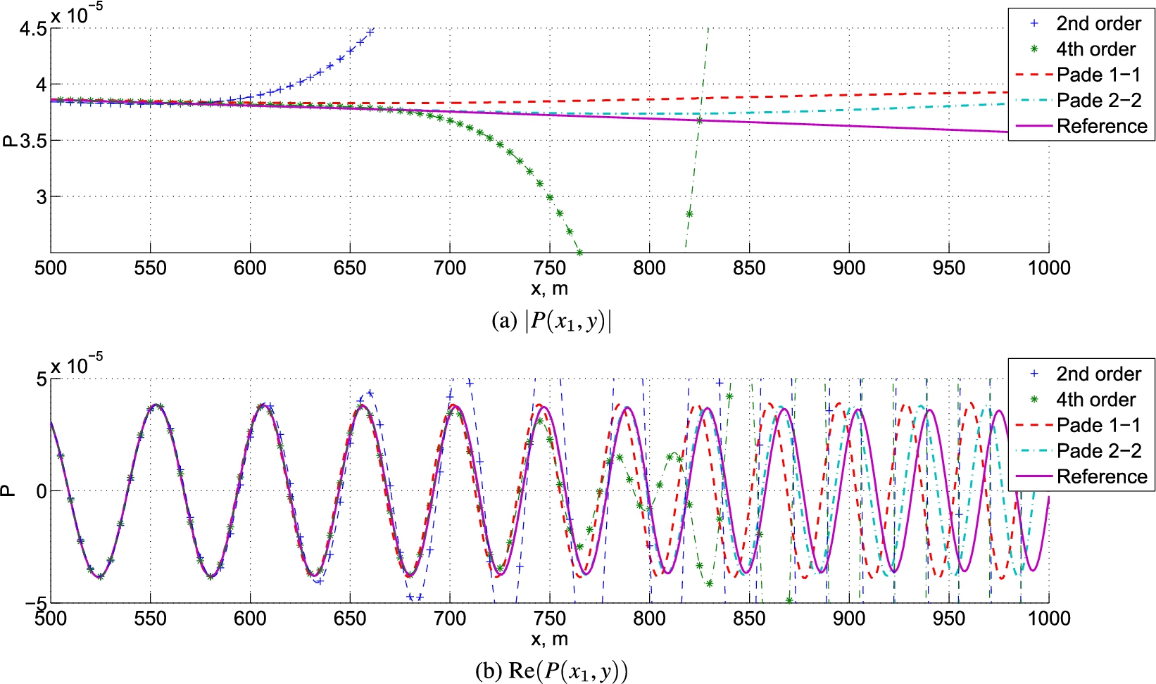
Fundamental solution of the Helmholtz equation (6), its iterative parabolic approximations of orders 2 and 4, and their Padé counterparts, i.e., 1–1 and 2–2 Padé approximations.

This phenomenon is illustrated in Fig. 1, where the fundamental solution of the Helmholtz equation is shown together with its 2nd- and 4th-order IPAs. In this example we consider an isovelocity medium with $c = 1500 m/s$ and source with the frequency of $f = 100 Hz$ (the source is located at $x = 0$ , $y = 0$ , $z = 0$ ). The wavenumber in is computed by the formula $k = 2 π f / c$ . The solution is shown as a function of y at $x = x_{1} = 2 km$ and $z = 0$ . Note that we compare the solutions for $y > y_{1} = 500 m$ , as they almost exactly coincide for $y < y_{1}$ . Although the 4th-order IPA is noticeably more accurate than its 2nd-order counterpart, it can be seen from Fig. 1(a) that for both of them the magnitude eventually experiences a polynomial growth in y and therefore strongly diverges from the reference solution. Hereafter we refer to this phenomenon as sidelobe divergence of IPAs.

In 2D practical problems of underwater acoustics the sidelobe divergence does not cause any serious problem, since the sidelobes of large magnitude leave the computational domain through the lower artificial boundary and hence do not affect the far field, cf. [9]. Theoretically, artificial boundary conditions can resolve this issue in a similar way in the 3D case. In practice they must be set at the lower horizontal boundary $z = z_{max}$ and artificial vertical boundaries $y = y_{1}$ and $y = y_{2}$ introduced for the truncation of the computational domain. For example, the conditions of Feshchenko and Popov [3] can be generalized to the IPE case to handle this problem.

In many cases however it can be more efficient to replace the polynomial series by an asymptotically equivalent sequence of rational functions. For example, it is known that one can use $2 N + 1$ Taylor coefficients in order to compute the coefficients of an N–N-Padé approximant. It is therefore clear that we can replace the partial sum corresponding to $u_{2 N}$ (i.e., $2 N$ -th order iterative parabolic approximation consisting of $2 N + 1$ terms) by its Padé equivalent $\begin{matrix} \sum_{j = 0}^{2 N + 1} ϵ^{j} A_{j} \sim A_{0} \frac{1 + \sum_{j = 1}^{N} ϵ^{j} B_{j}}{1 + \sum_{j = 1}^{N} ϵ^{j} C_{j}} . \end{matrix}$ Here ∼ means asymptotic equivalence, i.e., the equality modulo higher-order terms in ϵ. The functions $B_{j} (x, y)$ and $C_{j} (x, y)$ (the counterparts of $B_{j}$ and $C_{j}$ in physical variables) can be easily determined from a system of linear equations once the values $A_{j}$ are known. In the simplest case $N = 1$ the system has the form $\begin{matrix} \{\begin{matrix} A_{0} B_{1} - A_{0} C_{1} = A_{1}, \\ A_{1} C_{1} = - A_{2}, \end{matrix} \end{matrix}$ and therefore $C_{1} = - A_{2} / A_{1}$ , $B_{1} = A_{1} / A_{0} - A_{2} / A_{1}$ .

In the general case we can introduce an N–N iterative Padé approximation by replacing the truncated sum of $2 N + 1$ terms of the series (4) by the respective rational function $\begin{matrix} (25) & u \sim u_{N}^{P} = exp (i k_{0} x) A_{0} \frac{1 + \sum_{j = 1}^{N} B_{j}}{1 + \sum_{j = 1}^{N} C_{j}} . \end{matrix}$ By contrast to its IPA equivalent, the iterative Padé approximation, does not exhibit a polynomial growth at $y, z \to \infty$ . In Fig. 1 we present the 1–1 and 2–2 iterative Padé approximations that are equivalent to 2nd- and 4th-order IPAs, respectively. It can be seen that they no longer exhibit strong (polynomial) sidelobe divergence in the magnitude. At the same time, the quality of the phase approximation is almost identical for $u_{2 N}$ and $u_{N}^{P}$ .

In practice iterative Padé approximations can be obtained by solving the equations (5) and subsequently obtaining the functions $B_{j}$ and $C_{j}$ from a $2 N$ -by- $2 N$ linear system. Clearly, this does not substantially increase the computational complexity of the solution.

7. Example: Sound propagation in a perfect wedge

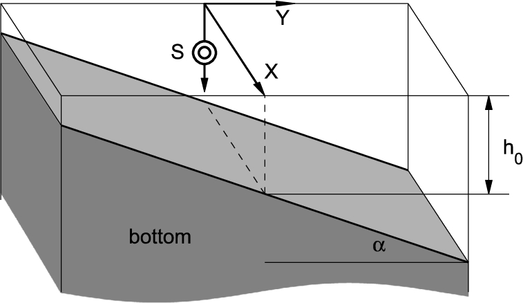
Since our main goal is to illustrate the accuracy of the point source representation by ICs for the system (5), we consider here a problem where both IPEs (5) and the Helmholtz equation (1) admit an analytical solution. In this example we perform the field computation for an idealized model of a coastal wedge formed by the sea surface $z = 0$ and the sloping bottom $z = h (y) = h_{0} + tan (α) y$ , where $h_{0}$ is the water depth at the source location and α is the slope angle of the bottom (see Fig. 2). The wedge $0 < z < h (y)$ is an isovelocity medium with the sound speed $c = 1500 m/s$ .

Fig. 2.

A coastal wedge-like waveguide. $z = 0$ represents sea surface.

We impose the pressure-release conditions $\begin{matrix} P |_{z = 0} = 0, P |_{z = h} = 0, \end{matrix}$ both at the surface and at the sea bottom (thus it is assumed that these boundaries are perfectly reflecting). While the pressure-release condition for the sea surface is routinely used in underwater acoustics, a perfectly reflecting bottom model is not adequate in most cases (the sea bottom must be considered penetrable instead). This simplification however allows us to obtain the solution analytically using the source images method for the Helmholtz equation [14]. In fact, such a scenario is not favorable for the parabolic equations theory (thus the calculations below can be considered as a worst-case benchmark). Indeed, in realistic models, with transparent or absorbing boundary conditions imposed at vertical artificial boundaries and the sea bottom, divergent sidelobes produced by the source and presenting an obstacle for the application of our method would quickly leave the domain. By contrast, in our example these sidelobes are trapped inside the wedge, as well as other waves with relatively large grazing angles. It is known that such waves present a challenge for parabolic equations.

In our example we set $α = 10^{\circ}$ , and $h_{0} = 200 m$ . The time-harmonic point source of the frequency $f = 100 Hz$ is located at $x = 0$ , $y = 0$ , $z = z_{s} = 100 m$ . Note that such a steep bottom slope can be also very difficult to handle in the framework of the parabolic equation theory. For the computation of the IPE solutions we set $σ = 1.5 / k$ in the initial conditions (18).

Fig. 3.

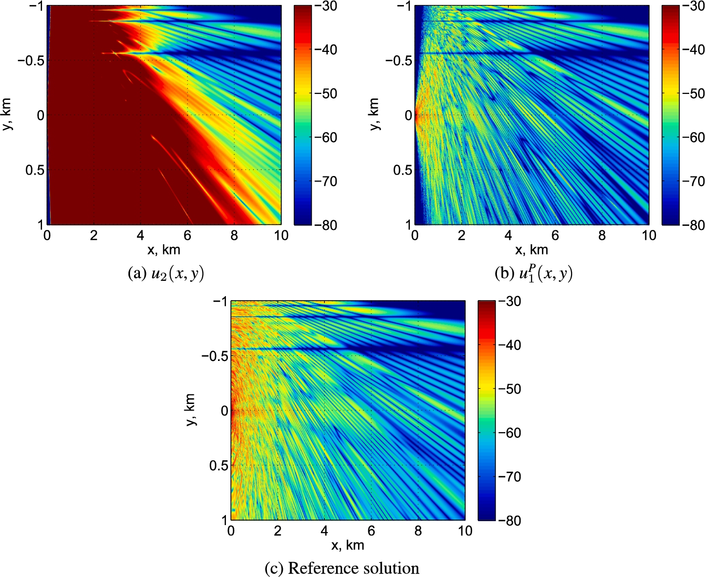
Sound field produced by a point source in a perfect 3D wedge.

Fig. 4.

Comparison of solutions presented in Fig. 3 along the line $z = 0$ , $x = 10 km$ .

We compute acoustic pressure levels (in dB re 1 m from the source) as a function of x, y in the plane $z = z_{s}$ . The computation results obtained using 2nd-order IPA, the respective 1–1-Padé approximation and the solution of the Helmholtz equation by the source images method are presented in Fig. 3. In this “worst case” scenario the 2nd-order IPA solution is totally crippled by the diverging sidelobes. These sidelobes however can be suppressed by using iterative Padé approximation as described in the previous section. We stress again that it takes only a very insignificant increase in the computational costs. A more detailed comparison of the three computed solutions is presented in Fig. 4, that shows the sound pressure levels along the line $z = 0$ , $x = 10 km$ . Although the agreement is not perfect for $y > 0.7 km$ , it is clear that the initial conditions proposed above do their job. This example also illustrates the capability of the regularization procedure outlined in the previous section.

8. Concluding remarks

In this study, we have derived the solution of the iterative parabolic equations corresponding to the fundamental solution of the Helmholtz equation. To our knowledge, the counterpart to this fundamental solution has not been identified in the “PE world” before. Moreover, we have also obtained Padé approximations to this fundamental solution and outlined a simple algorithm that can be used to transform Taylor-like IPA into its Padé counterpart. Such iterative Padé approximations allow one to solve the side-lobe divergence problem that spoils high-order IPE solutions. The Taylor-to-Padé transition discussed in Section 6 can be viewed as a regularization procedure for the IPA (4).

On the practical side, our study provides initial conditions for the solution of the Cauchy problem for IPE that allow us to simulate a wave field generated by a point source (i.e. to approximate the solution of the Helmholtz equation with the delta input term). In a sense, we have obtained the counterpart of the self-starter (see [2]) for IPE theory. Although one can easily fit starters designed for standard wide-angle PEs in 2D propagation problems, it has been unclear how to simulate the point source field in the 3D case. Therefore, in this study, we take another step towards a universal numerical model based on IPEs for solving 3D propagation problems of underwater acoustics.

Note that at this point we can only illustrate the capabilities of this approach in the 3D case on a very idealized test problem of sound propagation in a perfect wedge, where IPEs can be solved analytically using the source image technique. It would of course be desirable to provide a more convincing demonstration of the accuracy of the IPE-based propagation model by tackling a 3D problem with a penetrable wedge (as we did in [15] for the 2D case). However, this requires a significant amount of additional work, including the discretization of 3D boundary conditions in the case of inhomogeneous bathymetry [8], and the artificial domain truncation that can be achieved by deriving a generalization of the transparent boundary conditions from [3] to the IPE case. All these issues will be the subject of our future work.

Footnotes

Acknowledgements

This study was supported by the Russian Foundation for Basic Research under the contracts No. 18-05-00057_a and No. 18-35-20081_mol_a_ved. P.P. was also partly supported by the POI FEBRAS Program “Mathematical simulation and analysis of dynamical processes in the ocean” (No. 0271-2019-0001). P.P. was also partly supported by the Heinrich Hertz Stiftung.

References

J.F.

Claerbout, Fundamentals of Geophysical Data Processing: With Applications to Petroleum Prospecting, Blackwell Scientific Publications, 1985.

M.D.

Collins, A self-starter for the parabolic equation method, J. Acoust. Soc. Amer. 92(4) (1992), 2069–2074. doi:10.1121/1.405258.

R.M.

Feshchenko and

A.V.

Popov, Exact transparent boundary condition for the parabolic equation in a rectangular computational domain, J. Opt. Soc. Am. A 28 (2011), 373–380. doi:10.1364/JOSAA.28.000373.

V.E.

Grikurov and

A.P.

Kiselev, Gaussian beams at large distances, Radiophys. & Quant. Electron. 29 (1986), 233–237. doi:10.1007/BF01037628.

F.B.

Jensen,

W.A.

Kuperman,

M.B.

Porter and

Schmidt, Computational Ocean Acoustics, Springer, New York, 2011.

Levy, Parabolic Equation Methods for Electromagnetic Wave Propagation, Vol. 45, IET, 2000.

A.H.

Nayfeh, Perturbation Methods, John Wiley & Sons, New York, 1973.

P.S.

Petrov, Three-dimensional iterative parabolic approximations, Proceedings of Meetings on Acoustics, 25 (2015), 070002.

P.S.

Petrov and

Ehrhardt, Transparent boundary conditions for iterative high-order parabolic equations, J. Comput. Phys. 313 (2016), 144–158. doi:10.1016/j.jcp.2016.02.037.

10.

P.S.

Petrov,

Ehrhardt,

A.G.

Tyshchenko and

P.N.

Petrov, Wide-angle mode parabolic equation with transparent boundary conditions and its applications in shallow water acoustics, Journal of Sound and Vibration (2020), submitted.

11.

P.S.

Petrov,

D.V.

Makarov and

Ehrhardt, Wide-angle parabolic approximations for the nonlinear Helmholtz equation in the Kerr media, EPL (Europhysics Letters) 116(2) (2016), 24004. doi:10.1209/0295-5075/116/24004.

12.

A.V.

Popov and

S.A.

Khozioskii, A generalization of the parabolic equation of diffraction theory, USSR Comput. Math. Math. Phys. 17(2) (1977), 238–244. doi:10.1016/0041-5553(77)90057-X.

13.

Richmyer, Principles of Advanced Mathematical Physics, Vol. I, Springer, New York, 1978.

14.

Tang,

Petrov,

Piao and

Kozitskiy, On the method of source images for the wedge problem solution in ocean acoustics: Some corrections and appendices, Acoustical Physics 64(2) (2018), 225–236. doi:10.1134/S1063771018020070.

15.

M.Y.

Trofimov,

P.S.

Petrov and

A.D.

Zakharenko, A direct multiple-scale approach to the parabolic equation method, Wave Motion 50(3) (2013), 586–595. doi:10.1016/j.wavemoti.2012.12.004.

16.

Wolfram Alpha, Pattern solver widget for Wolfram Alpha, https://www.wolframalpha.com/widgets/view.jsp?id=a3af2e675c3bfae0f2ecce820c2bef43, Accessed: 2020-04-27.