Existence of solution to a Cahn

Abstract

Our aim in this paper is to prove the existence to a Cahn–Hilliard equation with a proliferation term and endowed with Neumann boundary conditions. Such a model has, in particular, applications in biology. We first consider regular nonlinear term then logarithmic one. We finally give some numerical simulations which confirm the theoretical results.

Keywords

Cahn-Hilliard equation proliferation term regular nonlinear term logarithmic nonlinear term existence simulations

1. Introduction

The Cahn–Hilliard equation is a parabolic partial differential equation of the fourth order, introduced in 1958 by John W. Cahn and John E. Hilliard. It is a time evolution equation for the concentration of a material. It was proposed in order to describe phase separation processes (also known as spinodal decomposition) in binary alloy (see [4] and [5]). Spinodal decomposition is a process by which a mixture of two materials can separate into distinct regions with different material concentration [4].

However, the use of the Cahn–Hilliard equation has been extended to various areas of chemistry, physics and biology such as: population dynamics (see [9]), bacterial films (see [18]), thin films (see [26] and [27]), the rings of Saturn (see [28]), the clustering of mussels (see [20]), wound healing (see [17]), topology optimization (see [15] and [31]), image processing (see [3] and [6]) and tumor growth (see [7] and [16]).

In this article, we are interested in the following generalization of the Cahn–Hilliard equation: $\begin{matrix} (1) & \frac{\partial u}{\partial t} + Δ^{2} u - Δ f (u) + g (x, u) = 0 . \end{matrix}$ Here, u is the order parameter. Furthermore, f is the derivative of a double-well potential F. A thermodynamically relevant potential F is the following logarithmic function which follows from mean-field model: $\begin{matrix} F (s) = \frac{θ_{1}}{2} (1 - s^{2}) + \frac{θ_{2}}{2} [(1 - s) ln (\frac{1 - s}{2}) + (1 + s) ln (\frac{1 + s}{2})], s \in (- 1, 1), 0 < θ_{1} < θ_{2}, \end{matrix}$ i.e., $\begin{matrix} (2) & f (s) = - θ_{1} s + \frac{θ_{2}}{2} ln \frac{1 + s}{1 - s}, s \in (- 1, 1) . \end{matrix}$ Although such a function is very often approximated by regular ones, typically, $F (s) = \frac{1}{4} (s^{2} - 1)$ , i.e., $\begin{matrix} (3) & f (s) = s^{3} - s . \end{matrix}$ The function g in the above general equation has, in particular, the following possibilities:

The linear function $\begin{matrix} g (s) = α s, α > 0 . \end{matrix}$ In this case (5) is known as the Cahn–Hilliard-Oono equation account for long-ranged (nonlocal) interactions in the phase separation process (see [21,25] and [30]).

The quadratic function $\begin{matrix} g (s) = α s (s - 1), α > 0 . \end{matrix}$ In this case, (5) has application in biology (see [29] and [1]), more specifically, in tumor growth (see [7] and [16]) and wound healing (see [17]).

Fidelity term $\begin{matrix} g (x, s) = λ_{0} χ_{Ω / D} (s - h (x)), λ_{0} > 0, D \subset Ω, h \in L^{2} (Ω), \end{matrix}$ where χ denotes the indicator function. This function g was proposed in [2,3] in view of applications to binary image inpainting.

Another possibility, with application in biology, is the function $\begin{matrix} g (x, s) = \frac{λ_{1}}{2} (1 + s) - λ_{2} {(1 + s)}^{2} {(1 - s)}^{2} + h (x), \end{matrix}$ where $λ_{1}$ and $λ_{2}$ being constants which represent the growth coefficient and the death one, respectively. Here, the term $h (x)$ is used as an artificial growth term which allows us to manufacture a desired PDE solution, but it could also serve to model biologically relevant phenomenal.

The generalized equation (5) was studied in [12] and [22], when endowed with Dirichlet boundary condition. There, the well-posedness and asymptotic behavior of the associated system are studied. However, when considering the case of Neumann boundary conditions, the situation is different due to the fact that one no longer has the conservation of mass (see [11,12] and [7]).

In this paper, we consider the generalized Cahn–Hilliard equation (1) in view of applications in biology, more precisely, models wound healing and tumor growth, endowed with Neumann boundary conditions, with proliferation term $\begin{matrix} (4) & g (s) = \frac{λ_{1}}{2} (1 + s) - λ_{2} {(1 + s)}^{2} {(1 - s)}^{2}, λ_{1}, λ_{2} > 0, \end{matrix}$ here, the order parameter u is the local density of cells.

Similar generalizations of the Cahn–Hilliard equation are now well understood from a mathematical point of view. In particular, one has a rather complete picture as far as the existence, the uniqueness and the regularity of solutions and the asymptotic behavior of the system. We refer the reader to (among a huge literature), e.g., [8,10] and [24] for the logarithmic nonlinear term and to [7,11] and [23] for a regular nonlinear term.

This paper is organized as follows. In Section 2, we state our assumptions on the mathematical problem and give some useful notation. Then, in Section 3, we consider a regular nonlinear term. We prove the existence and uniqueness of local (in time) solution to the problem. In Section 4, we take f as a logarithmic function. We prove the existence of a local (in time) biologically relevant solution to the problem. Furthermore, we give a condition which ensure the existence of a global (in time) solution. Finally, in Section 5, we give some numerical simulations which confirm these results.

2. Setting of the problem and notation

We Consider the following initial and boundary value problem in a bounded regular domain $Ω \subset R^{n}$ , $n = 1$ , 2 or 3, with boundary Γ and ν is the outer unit normal to Γ: $\begin{matrix} (5) & \begin{array}{l} \frac{\partial u}{\partial t} + Δ^{2} u - Δ f (u) + g (x, u) = 0, in (0, T) \times Ω, \\ \frac{\partial u}{\partial ν} = \frac{\partial Δ u}{\partial ν} = 0, on (0, T) \times Γ, \\ u (0, x) = u_{0} (x), in Ω, \end{array} \end{matrix}$ where g is defined in (4).

Integrating (5) over Ω, we have $\begin{matrix} \frac{d}{d t} \int_{Ω} u d x + \int_{Ω} g (u) d x = 0, \end{matrix}$ hence $\begin{matrix} (6) & \frac{d}{d t} ⟨ u ⟩ + ⟨ g (u) ⟩ = 0 . \end{matrix}$ In Section 3, we consider a regular nonlinear term $f \in C^{2} (R)$ .

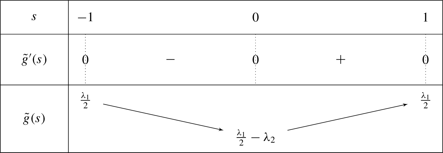
In Section 4, $f = F^{'}$ as defined in (2). Writing $F (s) = \frac{θ_{1}}{2} (1 - s^{2}) + F_{1} (s)$ and $f_{1} = F_{1}^{'}$ , we introduce, for $N \in N$ , the approximated function $F_{1, N} \in C^{8} (R)$ defined by $\begin{array}{l} \begin{matrix} F_{1, N}^{(8)} (s) = \{\begin{matrix} F_{1}^{(8)} (1 - \frac{1}{N}) & s ⩾ 1 - \frac{1}{N}, \\ F_{1}^{(8)} (s) & | s | ⩽ 1 - \frac{1}{N}, \\ F_{1}^{(8)} (- 1 + \frac{1}{N}) & s ⩽ - 1 + \frac{1}{N}, \end{matrix} \end{matrix} \\ F_{1, N}^{(k)} (0) = F_{1}^{(k)} (0), k = 0, 1, \dots, 8, \end{array}$ so that $\begin{matrix} F_{1, N} (s) = \{\begin{matrix} \sum_{k = 0}^{8} \frac{1}{k!} F_{1}^{(k)} (1 - \frac{1}{N}) {(s - 1 + \frac{1}{N})}^{k} & s ⩾ 1 - \frac{1}{N}, \\ F_{1} (s) & | s | ⩽ 1 - \frac{1}{N}, \\ \sum_{k = 0}^{8} \frac{1}{k!} F_{1}^{(k)} (- 1 + \frac{1}{N}) {(s - 1 + \frac{1}{N})}^{k} & s ⩽ - 1 + \frac{1}{N} . \end{matrix} \end{matrix}$ Setting $F_{N} (s) = \frac{θ_{1}}{2} (1 - s^{2}) + F_{1, N} (s)$ , $f_{1, N} = F_{1, N}^{'}$ and $f_{N} = F_{N}^{'}$ , there holds (see [14]) $\begin{matrix} (7) & \begin{array}{l} f_{1, N}^{'} ⩾ 0, f_{N}^{'} ⩾ - θ_{1}, \\ F_{N} (s) ⩾ c_{1} s^{8} - c_{2}, s \in R, \\ f_{N} (s) s ⩾ c_{3} (F_{N} (s) + | f_{1, N} (s) |) - c_{4}, c_{3} > 0, c_{4} ⩾ 0, s \in R, \\ f_{N} (s + m) s ⩾ c_{5} (F_{N} (s + m) + | f_{1, N} (s + m) |) - c_{6}, c_{5} > 0, c_{6} ⩾ 0, s \in R, m \in (- 1, 1), \end{array} \end{matrix}$ where the constants $c_{i}$ , $i = 1, \dots, 6$ are independent of N, for N large enough.

Let $H : = L^{2} (Ω)$ and $V : = H^{1} (Ω)$ and denote by $‖ \cdot ‖$ , $(\cdot, \cdot)$ the norm and the scalar product in H, respectively.

We set $‖ \cdot ‖_{- 1} = ‖ {(- Δ)}^{- \frac{1}{2}} \cdot ‖$ , where ${(- Δ)}^{- 1}$ is the inverse minus Laplace operator associated with Neumann boundary conditions and acting on functions with null average. Furthermore, $‖ \cdot ‖_{X}$ denotes the norm in the Banach space X.

We set, for $v \in L^{1} (Ω)$ , $\begin{matrix} ⟨ v ⟩ = \frac{1}{Vol (Ω)} \int_{Ω} v d x, \end{matrix}$ and, for $v \in H^{- 1} (Ω)$ , $\begin{matrix} ⟨ v ⟩ = \frac{1}{Vol (Ω)} {⟨ v, 1 ⟩}_{H^{- 1} (Ω), H^{1} (Ω)} . \end{matrix}$ We finally set, whenever it makes sense, $\begin{matrix} \bar{v} = v - ⟨ v ⟩ . \end{matrix}$ We note that $\begin{array}{l} v \mapsto {(‖ \bar{v} ‖_{- 1}^{2} + {⟨ v ⟩}^{2})}^{\frac{1}{2}}, \\ v \mapsto {(‖ \bar{v} ‖^{2} + {⟨ v ⟩}^{2})}^{\frac{1}{2}}, \\ v \mapsto {(‖ \nabla v ‖^{2} + {⟨ v ⟩}^{2})}^{\frac{1}{2}}, \end{array}$ and $\begin{matrix} v \mapsto {(‖ Δ v ‖^{2} + {⟨ v ⟩}^{2})}^{\frac{1}{2}}, \end{matrix}$ are norms in $H^{- 1} (Ω)$ , $L^{2} (Ω)$ , $H^{1} (Ω)$ , and $H^{2} (Ω)$ , respectively, which are equivalent to the usual ones.

Throughout this article, the same letter c denotes a constant which may vary from line to line, or even in the same line. Similarly, the same letter Q denotes a monotone increasing function which may vary from line to line, or even in the same line.

3. Regular nonlinear term

Theorem 3.1.
We assume that $u_{0} \in H^{2} (Ω)$ . Then, there exists $T > 0$ and a unique weak solution u of ( 5 ) such that $u \in L^{2} (0, T; H^{4} (Ω))$ and $\frac{\partial u}{\partial t} \in L^{2} (0, T; L^{2} (Ω))$ .
Proof.
We proceed by first proving the existence of such a solution and then showing the uniqueness of it.

Existence. The existence proof is based on Faedo–Galerkin method, a priori estimates and compactness method.

We start with a weak formulation of the Cahn–Hilliard equation.

A solution of problem (5) is a function u such that $u \in L^{2} (0, T; H^{2} (Ω))$ , $\frac{\partial u}{\partial ν} |_{Γ} = 0$ and satisfying the following weak formulation for a.e. $t \in (0, T)$ $\begin{matrix} (8) & \int_{Ω} \frac{\partial u}{\partial t} ϕ d x + \int_{Ω} Δ u Δ ϕ d x + \int_{Ω} \nabla f (u) \cdot \nabla ϕ d x + \int_{Ω} g (u) ϕ d x = 0, \end{matrix}$ for all $ϕ \in {ψ \in H^{2} (Ω), \frac{\partial ψ}{\partial ν} |_{\partial Ω} = 0}$ .

Step 1: Construction of the basis. We introduce the Riesz isomorphism $B : V \to V^{'}$ associated to the standard scalar product of V, that is $\begin{matrix} ⟨ B u, v ⟩ : = {(u, v)}_{V} = \int_{Ω} (\nabla u \cdot \nabla v + u v) for u, v \in V . \end{matrix}$ We notice that $B u = - Δ u + u if u \in D (B) : = {ϕ \in H^{2} (Ω) : \frac{\partial ϕ}{\partial ν} = 0 on \partial Ω}$ and that the restriction of B to $D (B)$ is an isomorphism from $D (B)$ onto H.

By a classical spectral theorem there exist a sequence of eigenvalues $λ_{m}$ with $0 < λ_{1} ⩽ λ_{2} ⩽ \dots$ and $λ_{m} \to \infty$ , and a family of eigenfunctions $w_{m} \in D (B)$ such that $B w_{m} = λ_{m} w_{m}$ . The family of $w_{m}$ is an orthonormal basis in H and it is also orthogonal in V and $D (B)$ .

We set the space $\begin{matrix} V_{m} = span {w_{1}, \dots, w_{m}}, V_{\infty} = ⋃_{m = 1}^{\infty} V_{m}, \end{matrix}$ where $V_{\infty}$ is dense subspace of V.

Step 2: Construction of approximate solution. For any $m \in N$ , we are looking for functions of the form $u_{m} = \sum_{k = 1}^{m} d_{k} (t) w_{k}$ , solving the approximate regularized problem: $\begin{matrix} (9) & \int_{Ω} \frac{\partial u_{m}}{\partial t} w_{k} d x + \int_{Ω} Δ u_{m} Δ w_{k} d x + \int_{Ω} \nabla f (u_{m}) \cdot \nabla w_{k} d x + \int_{Ω} g (u) w_{k} d x = 0, \end{matrix}$ where $w_{k} \in V_{m}$ .

We aim to apply standard existence theorems for ODEs. For this purpose, if m is fixed, we obtain the following ODE system, having as unknowns the columns vectors $d = d_{m} = {(d_{k})}_{k = 1}^{m}$ : $\begin{matrix} (10) & A_{m} d^{'} = B_{m} d + F_{m} d + G_{m}, \end{matrix}$ where $A_{m} = {({(w_{k}, w_{l})}_{L^{2} (Ω)})}_{1 ⩽ k, l ⩽ m}$ , $B_{m} = {(- {(Δ w_{k}, Δ w_{l})}_{L^{2} (Ω)})}_{1 ⩽ k, l ⩽ m}$ , $F_{m} = {(- f^{'} (u_{m}) {(\nabla w_{k}, \nabla w_{l})}_{L^{2} (Ω)})}_{1 ⩽ k, l ⩽ m}$ and $G_{m} = {(- {(g (u_{m}), w_{k})}_{L^{2} (Ω)})}_{1 ⩽ k ⩽ m}$ . We have, $A_{m}$ is invertible, so System (10) may be written as $\begin{matrix} (11) & d^{'} = A_{m}^{- 1} H = h (t, d), \end{matrix}$ where H assembles the right hand side of system (10).

Moreover, the problem that we obtained is supplemented with initial condition $u_{0, m}$ the projection of $u_{0}$ onto $V_{m}$ .

We have $t ⟼ h (t, y)$ is measurable with respect to t and for all $R > 0$ there exists a function $F_{R} \in L^{1} (0, T)$ such that ${sup}_{y \in R^{m}, ‖ y ‖ ⩽ R} ‖ h (t, y) ‖_{R^{m}} ⩽ F_{R} (t)$ a.e. t.

Then, the theorem of existence of Caratheodory implies the local existence of solution $u_{m}$ .

Step 3: Energy estimates. Note that the Galerkin solution satisfies the following weak formulation: $\begin{matrix} (12) & \int_{Ω} \frac{\partial u_{m}}{\partial t} ϕ_{m} d x + \int_{Ω} Δ u_{m} Δ ϕ_{m} d x + \int_{Ω} \nabla f (u_{m}) \cdot \nabla ϕ_{m} + \int_{Ω} g (u_{m}) ϕ_{m} d x = 0, \end{matrix}$ where the function $ϕ_{m} (t, x) = \sum_{k = 1}^{m} a_{k} (t) w_{k} (x)$ .

Now, substituting $ϕ_{m} = Δ^{2} u_{m}$ in (12), we obtain: $\begin{matrix} \frac{1}{2} \frac{d}{d t} ‖ Δ u_{m} ‖^{2} + {‖ Δ^{2} u_{m} ‖}^{2} ⩽ \frac{1}{2} {‖ Δ^{2} u_{m} ‖}^{2} + {‖ Δ f (u_{m}) ‖}^{2} + {‖ g (u_{m}) ‖}^{2}, \end{matrix}$ which yields, $\begin{matrix} \frac{d}{d t} ‖ Δ u_{m} ‖^{2} + {‖ Δ^{2} u_{m} ‖}^{2} ⩽ c ({‖ f (u_{m}) ‖}_{H^{2} (Ω)}^{2} + {‖ g (u_{m}) ‖}^{2}) . \end{matrix}$ Using $H^{2} (Ω)$ continuously embedded in $C (\bar{Ω})$ , we have $\begin{matrix} {‖ f (u_{m}) ‖}_{H^{2} (Ω)}^{2} + {‖ g (u_{m}) ‖}^{2} ⩽ Q (‖ u_{m} ‖_{H^{2} (Ω)}^{2}) . \end{matrix}$ Furthermore, using ${(‖ Δ u ‖^{2} + {⟨ u ⟩}^{2})}^{\frac{1}{2}}$ equivalent to the usual norm in $H^{2} (Ω)$ and $\begin{matrix} \frac{d}{d t} {⟨ u_{m} ⟩}^{2} = 2 ⟨ u_{m} ⟩ \frac{d}{d t} ⟨ u_{m} ⟩ = - 2 ⟨ u_{m} ⟩ ⟨ g (u_{m}) ⟩ ⩽ c (‖ u_{m} ‖^{2} + {‖ g (u_{m}) ‖}^{2}) ⩽ Q (‖ u_{m} ‖_{H^{2} (Ω)}^{2}), \end{matrix}$ we obtain $\begin{matrix} \frac{d}{d t} ‖ u_{m} ‖_{H^{2} (Ω)}^{2} + {‖ Δ^{2} u_{m} ‖}^{2} ⩽ Q (‖ u_{m} ‖_{H^{2} (Ω)}^{2}) . \end{matrix}$ Setting $y = ‖ u_{m} ‖_{H^{2} (Ω)}^{2}$ , we deduce $y^{'} ⩽ Q (y)$ .

Let z be the solution to the ordinary differential equation $z^{'} = Q (z)$ , $z (0) = y (0)$ .

It follows from the comparison principle that there exists $T > 0$ , which is independent of m, such that $\begin{matrix} y (t) ⩽ z (t), \forall t \in [0, T] . \end{matrix}$ Hence, $\begin{matrix} (13) & {‖ u_{m} (t) ‖}_{H^{2} (Ω)}^{2} + {‖ Δ^{2} u_{m} (t) ‖}^{2} ⩽ c, \forall t \in [0, T] . \end{matrix}$ We assume from now on that $t \in [0, T]$ .

Moreover, one can obtain some uniform estimates on the time derivative as follows.

Substitute $ϕ_{m} = \frac{\partial u_{m}}{\partial t}$ in (12), we obtain $\begin{matrix} {‖ \frac{\partial u_{m}}{\partial t} ‖}^{2} + \frac{1}{2} \frac{d}{d t} ‖ Δ u_{m} ‖^{2} = (Δ f (u_{m}), \frac{\partial u_{m}}{\partial t}) - (g (u_{m}), \frac{\partial u_{m}}{\partial t}), \end{matrix}$ using Young’s inequality yields: $\begin{matrix} {‖ \frac{\partial u_{m}}{\partial t} ‖}^{2} + \frac{d}{d t} ‖ Δ u_{m} ‖^{2} ⩽ c . \end{matrix}$ Integrating in time between 0 and t, we deduce: $\begin{matrix} (14) & \int_{0}^{t} {‖ \frac{\partial u_{m}}{\partial t} (s) ‖}^{2} d s + {‖ Δ u_{m} (t) ‖}^{2} ⩽ c t + ‖ Δ u_{m, 0} ‖^{2} . \end{matrix}$ We get $\begin{matrix} (15) & \int_{0}^{t} {‖ \frac{\partial u_{m}}{\partial t} (s) ‖}^{2} < \infty, \forall t \in [0, T] . \end{matrix}$

Step 4: Passage to the limit and existence of solution. From (13), one can see that $(u_{m})$ is bounded in $L^{2} (0, T; V)$ . Moreover, we deduce from (15) that $(\frac{\partial u_{m}}{\partial t})$ is bounded in $L^{2} (0, T; H)$ . Then, by the Aubin-Lions compactness result, we can assume that there exist limit function $u \in L^{2} (0 . T; H)$ such that as $m \to + \infty$ , $\begin{matrix} u_{m} \to u strongly in L^{2} (0, T; H) and a.e. . \end{matrix}$ Since $f (u)$ is regular, $g (u)$ is a polynomial, and using $u_{m} \to u$ a.e. in $(0, T) \times H$ , we obtain $\begin{array}{l} f (u_{m} (x, t)) \to f (u (x, t)), Δ f (u_{m} (x, t)) \to Δ f (u (x, t)) and \\ g (u_{m} (x, t)) \to g (u (x, t)) a.e. in (0, T) \times H . \end{array}$ On the other hand, we have $Δ f (u_{m} (x, t))$ and $g (u_{m} (x, t))$ are bounded in $L^{2} (0, T; H)$ . Then, $\begin{matrix} Δ f (u_{m}) \to Δ f (u), and g (u_{m}) \to g (u) weakly in L^{2} (0, T; H) (see [19]) . \end{matrix}$ We can pass to the limit in the approximated problem.

Uniqueness. Note that (5) is equivalent to $\begin{matrix} {(- Δ)}^{- 1} \frac{\partial}{\partial t} (u - ⟨ u ⟩) - Δ u + f (u) - ⟨ f (u) ⟩ + {(- Δ)}^{- 1} (g (u) - ⟨ g (u) ⟩) = 0 . \end{matrix}$ Suppose that $u_{1}$ and $u_{2}$ are two different solutions to (5) with initial data $u_{1, 0}$ and $u_{2, 0}$ respectively. Then, $u = u_{1} - u_{2}$ and $u_{0} = u_{1, 0} - u_{2, 0}$ satisfy: $\begin{array}{l} \frac{d}{d t} {(- Δ)}^{- 1} \bar{u} - Δ u + f (u_{1}) - f (u_{2}) - ⟨ f (u_{1}) - f (u_{2}) ⟩ \\ + {(- Δ)}^{- 1} (g (u_{1}) - g (u_{2}) - ⟨ g (u_{1}) - g (u_{2}) ⟩) = 0 . \end{array}$ Multiplying by $\bar{u}$ , we get $\begin{array}{l} \frac{1}{2} \frac{d}{d t} ‖ \bar{u} ‖_{- 1}^{2} + ‖ \nabla u ‖^{2} + (f (u_{1}) - f (u_{2}), \bar{u}) \\ + ({(- Δ)}^{- 1} (g (u_{1}) - g (u_{2}) - ⟨ g (u_{1}) - g (u_{2}) ⟩), \bar{u}) = 0 . \end{array}$ We have $\begin{matrix} (f (u_{1}) - f (u_{2}), \bar{u}) & = ({(- Δ)}^{\frac{1}{2}} (f (u_{1}) - f (u_{2})), {(- Δ)}^{- \frac{1}{2}} \bar{u}) \\ ⩽ c ‖ {(- Δ)}^{- \frac{1}{2}} \bar{u} ‖ ‖ {(- Δ)}^{\frac{1}{2}} (f (u_{1}) - f (u_{2})) ‖ \\ ⩽ c (‖ \bar{u} ‖_{- 1}^{2} + {‖ \nabla (f (u_{1}) - f (u_{2})) ‖}^{2}) . \end{matrix}$ Using $f (u_{1}) - f (u_{2}) = u \int_{0}^{1} f^{'} (s u_{1} + (1 - s) u_{2}) d s$ , we find $\begin{array}{rcl} ‖ \nabla (f (u_{1}) - f (u_{2})) ‖ & = & ‖ \nabla (u \int_{0}^{1} f^{'} (s u_{1} + (1 - s) u_{2}) d s) ‖ \\ = & ‖ \nabla u \int_{0}^{1} f^{'} (s u_{1} + (1 - s) u_{2}) d s \\ + u \int_{0}^{1} f^{″} (s u_{1} + (1 - s) u_{2}) (s \nabla u_{1} + (1 - s) \nabla u_{2}) d s ‖ \\ ⩽ & c (‖ \nabla u ‖ + ‖ u \nabla u_{1} ‖ + ‖ u \nabla u_{2} ‖) \\ ⩽ & c ‖ \nabla u ‖ . \end{array}$ We note that $\begin{matrix} | ({(- Δ)}^{- 1} (g (u_{1}) - g (u_{2}) - ⟨ g (u_{1}) - g (u_{2}) ⟩), \bar{u}) | \\ ⩽ ‖ \bar{u} ‖_{- 1} ‖ g (u_{1}) - g (u_{2}) ‖ \\ ⩽ ‖ \bar{u} ‖_{- 1} {(\int_{Ω} | u |^{2} {(\int_{0}^{1} g^{'} (s u_{1} + (1 - s) u_{2}) d s)}^{2} d x)}^{\frac{1}{2}} \\ ⩽ c ‖ \bar{u} ‖_{- 1} {(\int_{Ω} | u |^{2} {(\int_{0}^{1} (1 + {(s u_{1} + (1 - s) u_{2})}^{4}) d s)}^{2} d x)}^{\frac{1}{2}} \\ ⩽ c ‖ \bar{u} ‖_{- 1} {(\int_{Ω} | u |^{2} {(1 + | u_{1} |^{4} + | u_{2} |^{4})}^{2} d x)}^{\frac{1}{2}} \\ ⩽ c Q (‖ u_{1, 0} ‖_{H^{2} (Ω)}, ‖ u_{2, 0} ‖_{H^{2} (Ω)}) ‖ \bar{u} ‖_{- 1} ‖ u ‖ \\ ⩽ c (‖ \bar{u} ‖_{- 1}^{2} + ‖ u ‖^{2}), \end{matrix}$ and $\begin{matrix} \frac{d}{d t} {⟨ u ⟩}^{2} = 2 ⟨ u ⟩ \frac{d}{d t} ⟨ u ⟩ = - 2 ⟨ u ⟩ ⟨ g (u_{1}) - g (u_{2}) ⟩ ⩽ c (‖ u ‖^{2} + {‖ g (u_{1}) - g (u_{2}) ‖}^{2}) . \end{matrix}$ We have $\begin{array}{rcl} ‖ u ‖^{2} & ⩽ & 2 (‖ \bar{u} ‖^{2} + {⟨ u ⟩}^{2}) ⩽ c (‖ \bar{u} ‖_{- 1} ‖ \nabla u ‖ + {⟨ u ⟩}^{2}) \\ (16) & ⩽ & γ ‖ \nabla u ‖^{2} + c (‖ \bar{u} ‖_{- 1}^{2} + {⟨ u ⟩}^{2}), \forall γ > 0 . \end{array}$ Then $\begin{matrix} \frac{d}{d t} (‖ \bar{u} ‖_{- 1}^{2} + {⟨ u ⟩}^{2}) + c ‖ \nabla u ‖^{2} ⩽ c^{'} (‖ \bar{u} ‖_{- 1}^{2} + {⟨ u ⟩}^{2}) . \end{matrix}$ Finally, using Gronwall’s lemma yields, the continuous dependence with respect to the initial data in the $H^{- 1} (Ω)$ -norm, and the uniqueness holds. □
Lemma 3.1.
Let u be a solution to ( 5 ). Then $⟨ u ⟩$ is bounded from below.
Proof.
We note that $\begin{matrix} u^{4} - 2 u^{2} ⩾ - 1 . \end{matrix}$ It follows from (6) that $\begin{matrix} \frac{d ⟨ u ⟩}{d t} + \frac{λ_{1}}{2} ⟨ u ⟩ ⩾ - \frac{λ_{1}}{2}, \end{matrix}$ hence $\begin{matrix} \frac{d}{d t} (e^{\frac{λ_{1}}{2} t} ⟨ u ⟩) ⩾ - \frac{λ_{1}}{2} e^{\frac{λ_{1}}{2} t} . \end{matrix}$ It thus follows that $\begin{matrix} ⟨ u (t) ⟩ ⩾ (⟨ u_{0} ⟩ + 1) e^{- \frac{λ_{1}}{2} t}, t \in [0, T], \end{matrix}$ i.e., $⟨ u ⟩$ is bounded from below. □
4. Logarithmic nonlinear term

We now introduce, for $N \in N$ , the approximated problem $\begin{matrix} (17) & \begin{matrix} \frac{\partial u_{N}}{\partial t} + Δ^{2} u_{N} - Δ f_{N} (u_{N}) + g (u_{N}) = 0, \\ \frac{\partial u_{N}}{\partial ν} = \frac{\partial Δ u_{N}}{\partial ν} = 0 on Γ, \\ u_{N} |_{t = 0} = u_{0} . \end{matrix} \end{matrix}$ It follows from the previous section that we have the existence, uniqueness and regularity (depending on the regularity of $u_{0}$ ) of the local in time solution $u_{N}$ to (17).

All constants below are independent of the approximation parameter N.

We rewrite the problem in the following equivalent weak form: $\begin{matrix} (18) & \begin{matrix} {(- Δ)}^{- 1} \frac{\partial {\overline{u}}_{N}}{\partial t} - Δ {\overline{u}}_{N} + \overline{f_{N} (u_{N})} + {(- Δ)}^{- 1} \overline{g (u_{N})} = 0, \\ \frac{\partial {\overline{u}}_{N}}{\partial ν} = 0 on Γ, \\ {\overline{u}}_{N} |_{t = 0} = \overline{u_{0}} . \end{matrix} \end{matrix}$

Lemma 4.1.
Let $u_{N}$ be a solution to ( 18 ). Then, there exists $T > 0$ , which is independent of N, such that $\begin{matrix} (19) & {‖ {\overline{u}}_{N} (t) ‖}^{2} ⩽ c and {‖ {\overline{u}}_{N} (t) ‖}_{- 1}^{2} ⩽ c, t \in [0, T] . \end{matrix}$ Moreover, we assume that there exists $δ \in (0, \frac{1}{2}]$ such that $\begin{matrix} (20) & | ⟨ u_{0} ⟩ | ⩽ 1 - 2 δ, \end{matrix}$ then, for $t \in [0, T]$ $\begin{matrix} | ⟨ u_{N} ⟩ | ⩽ 1 - δ . \end{matrix}$
Proof.
Multiplying (18) by ${\overline{u}}_{N}$ and integrating over Ω, we have $\begin{matrix} \frac{1}{2} \frac{d}{d t} ‖ {\overline{u}}_{N} ‖_{- 1}^{2} + ‖ \nabla {\overline{u}}_{N} ‖^{2} + (\overline{f_{N} (u_{N})}, {\overline{u}}_{N}) + (\overline{g (u_{N})}, {(- Δ)}^{- 1} {\overline{u}}_{N}) = 0 . \end{matrix}$ Note that $\begin{matrix} (\overline{f_{N} (u_{N})}, {\overline{u}}_{N}) & = (f_{N} (u_{N}) - f_{N} (⟨ u_{N} ⟩), {\overline{u}}_{N}) \\ = \int_{Ω} {\overline{u}}_{N}^{2} \int_{0}^{1} f_{N}^{'} (s u_{N} + (1 - s) ⟨ u_{N} ⟩) d s d x \\ ⩾ \int_{Ω} {\overline{u}}_{N}^{2} \int_{0}^{1} c {(s {\overline{u}}_{N} + ⟨ u_{N} ⟩)}^{6} d s d x - c ‖ {\overline{u}}_{N} ‖^{2} \\ ⩾ \int_{Ω} c ({\overline{u}}_{N}^{8} + \sum_{j = 1}^{6} {\overline{u}}_{N}^{7 - (j - 1)} {⟨ u_{N} ⟩}^{j}) d x - c ‖ {\overline{u}}_{N} ‖^{2}, \end{matrix}$ and $\begin{matrix} | \int_{Ω} (\sum_{j = 1}^{6} {\overline{u}}_{N}^{7 - (j - 1)} {⟨ u_{N} ⟩}^{j}) d x | ⩽ c \int_{Ω} {\overline{u}}_{N}^{8} d x + Q ({⟨ u_{N} ⟩}^{2}) . \end{matrix}$ Furthermore, $\begin{matrix} (\overline{g (u_{N})}, {(- Δ)}^{- 1} {\overline{u}}_{N}) & = (g (u_{N}) - g (⟨ u_{N} ⟩), {(- Δ)}^{- 1} {\overline{u}}_{N}) \\ ⩽ c (‖ {\overline{u}}_{N} ‖_{- 1}^{2} + {‖ g (u_{N}) - g (⟨ u_{N} ⟩) ‖}^{2}), \end{matrix}$ note that $\begin{matrix} {‖ g (u_{N}) - g (⟨ u_{N} ⟩) ‖}^{2} & ⩽ \int_{Ω} {\overline{u}}_{N}^{2} \int_{0}^{1} {(g^{'} (s {\overline{u}}_{N} + ⟨ u_{N} ⟩))}^{2} d s d x \\ ⩽ c \int_{Ω} {\overline{u}}_{N}^{2} ({\overline{u}}_{N}^{6} + {\overline{u}}_{N}^{2} + {⟨ u_{N} ⟩}^{6} + {⟨ u_{N} ⟩}^{2} + c) d x \\ ⩽ c \int_{Ω} {\overline{u}}_{N}^{8} d x + Q ({⟨ u_{N} ⟩}^{2}) . \end{matrix}$ It follows that $\begin{matrix} (21) & \frac{d}{d t} ‖ {\overline{u}}_{N} ‖_{- 1}^{2} + ‖ \nabla {\overline{u}}_{N} ‖^{2} + c \int_{Ω} {\overline{u}}_{N}^{8} d x ⩽ Q ({⟨ u_{N} ⟩}^{2}) + c ‖ {\overline{u}}_{N} ‖_{- 1}^{2} . \end{matrix}$ Next, multiplying (18) by $- Δ {\overline{u}}_{N}$ , we obtain $\begin{matrix} \frac{1}{2} \frac{d}{d t} ‖ {\overline{u}}_{N} ‖^{2} + ‖ Δ {\overline{u}}_{N} ‖^{2} + (\overline{f_{N} (u_{N})}, - Δ {\overline{u}}_{N}) + (\overline{g (u_{N})}, {\overline{u}}_{N}) = 0 . \end{matrix}$ It follows from (7) $\begin{matrix} (\overline{f_{N} (u_{N})}, - Δ {\overline{u}}_{N}) = (f_{N}^{'} (u_{N}) \nabla {\overline{u}}_{N}, \nabla {\overline{u}}_{N}) ⩾ - c ‖ \nabla {\overline{u}}_{N} ‖^{2} ⩾ - c (‖ {\overline{u}}_{N} ‖^{2} + ‖ Δ {\overline{u}}_{N} ‖^{2})), \end{matrix}$ and, we have $\begin{matrix} | (\overline{g (u_{N})}, {\overline{u}}_{N}) | ⩽ c (‖ {\overline{u}}_{N} ‖^{2} + {‖ g (u_{N}) - g (⟨ u_{N} ⟩) ‖}^{2}) ⩽ c (‖ {\overline{u}}_{N} ‖^{2} + \int_{Ω} {\overline{u}}_{N}^{8} d x) + Q ({⟨ u_{N} ⟩}^{2}), \end{matrix}$ which yields $\begin{matrix} (22) & \frac{d}{d t} ‖ {\overline{u}}_{N} ‖^{2} + ‖ Δ {\overline{u}}_{N} ‖^{2} ⩽ Q ({⟨ u_{N} ⟩}^{2}) + c (‖ {\overline{u}}_{N} ‖^{2} + \int_{Ω} {\overline{u}}_{N}^{8} d x) . \end{matrix}$ Using (6), we obtain $\begin{matrix} (23) & \frac{d}{d t} {⟨ u_{N} ⟩}^{2} = - 2 ⟨ u_{N} ⟩ ⟨ g (u_{N}) ⟩ ⩽ Q ({⟨ u_{N} ⟩}^{2}) + c \int_{Ω} {\overline{u}}_{N}^{8} d x . \end{matrix}$ Summing (21), (22) and (23), we find $\begin{matrix} (24) & \begin{array}{l} \frac{d}{d t} (‖ {\overline{u}}_{N} ‖_{- 1}^{2} + ‖ {\overline{u}}_{N} ‖^{2} + {⟨ u_{N} ⟩}^{2}) + ‖ Δ {\overline{u}}_{N} ‖^{2} + ‖ \nabla {\overline{u}}_{N} ‖^{2} + c \int_{Ω} {\overline{u}}_{N}^{8} d x \\ ⩽ Q ({⟨ u_{N} ⟩}^{2}) + c (‖ {\overline{u}}_{N} ‖_{- 1}^{2} + ‖ {\overline{u}}_{N} ‖^{2}) . \end{array} \end{matrix}$ We deduce from (24) and from the comparison principle that there exists $T > 0$ , which is independent of N, such that $\begin{matrix} (25) & {‖ {\overline{u}}_{N} (t) ‖}^{2} ⩽ c, {‖ {\overline{u}}_{N} (t) ‖}_{- 1}^{2} ⩽ c, t \in [0, T] . \end{matrix}$ Finally, it follows from (20), (6) and (24) that, for $t \in [0, T]$ $\begin{matrix} | ⟨ u_{N} ⟩ | ⩽ 1 - δ . \end{matrix}$ □
Lemma 4.2.
Let $u_{N}$ be a solution to ( 18 ). Then, for $t \in [0, T]$ , $\begin{matrix} (26) & \frac{d}{d t} (‖ \nabla {\overline{u}}_{N} ‖^{2} + \int_{Ω} F_{N} (u_{N}) d x) + {‖ \frac{\partial {\overline{u}}_{N}}{\partial t} ‖}_{- 1}^{2} ⩽ c {‖ f_{N} (u_{N}) ‖}_{L^{1} (Ω)} . \end{matrix}$
Proof.
Multiplying (18) by ${\overline{u}}_{N}$ , we have $\begin{matrix} \frac{1}{2} \frac{d}{d t} ‖ {\overline{u}}_{N} ‖_{- 1}^{2} + ‖ \nabla {\overline{u}}_{N} ‖^{2} + (\overline{f_{N} (u_{N})}, {\overline{u}}_{N}) ⩽ c \int_{Ω} {\overline{u}}_{N}^{8} d x + c . \end{matrix}$ Noting that $\begin{matrix} (\overline{f_{N} (u_{N})}, {\overline{u}}_{N}) & = \frac{1}{2} (f_{N} (u_{N}), {\overline{u}}_{N}) + \frac{1}{2} (f_{N} (u_{N}) - f_{N} (⟨ u_{N} ⟩), {\overline{u}}_{N}) \\ ⩾ c ({‖ f_{N} (u_{N}) ‖}_{L^{1} (Ω)} + \int_{Ω} F_{N} (u_{N}) d x + \int_{Ω} {\overline{u}}_{N}^{8} d x) - c, \end{matrix}$ yields $\begin{matrix} (27) & \frac{d}{d t} ‖ {\overline{u}}_{N} ‖_{- 1}^{2} + c (‖ \nabla {\overline{u}}_{N} ‖^{2} + {‖ f_{N} (u_{N}) ‖}_{L^{1} (Ω)} + \int_{Ω} F_{N} (u_{N}) d x + \int_{Ω} {\overline{u}}_{N}^{8} d x) ⩽ c . \end{matrix}$ Now, multiplying (18) by $\frac{\partial {\overline{u}}_{N}}{\partial t}$ , we obtain $\begin{matrix} \frac{1}{2} \frac{d}{d t} ‖ \nabla {\overline{u}}_{N} ‖^{2} + {‖ \frac{\partial {\overline{u}}_{N}}{\partial t} ‖}_{- 1}^{2} + (f_{N} (u_{N}), \frac{\partial {\overline{u}}_{N}}{\partial t}) + (g (u_{N}) - g (⟨ u_{N} ⟩), {(- Δ)}^{- 1} \frac{\partial {\overline{u}}_{N}}{\partial t}) = 0 . \end{matrix}$ Furthermore, $\begin{matrix} (f_{N} (u_{N}), \frac{\partial {\overline{u}}_{N}}{\partial t}) & = (f_{N} (u_{N}), \frac{\partial u_{N}}{\partial t}) - (f_{N} (u_{N}), \frac{\partial ⟨ u_{N} ⟩}{\partial t}) \\ = \frac{d}{d t} \int_{Ω} F_{N} (u_{N}) d x + (f_{N} (u_{N}), ⟨ g (u_{N}) ⟩) \\ = \frac{d}{d t} \int_{Ω} F_{N} (u_{N}) d x + Vol (Ω) ⟨ f_{N} (u_{N}) ⟩ ⟨ g (u_{N}) ⟩ \\ ⩾ \frac{d}{d t} \int_{Ω} F_{N} (u_{N}) d x - c {‖ f_{N} (u_{N}) ‖}_{L^{1} (Ω)} {‖ g (u_{N}) ‖}^{2} . \end{matrix}$ It thus follows that $\begin{matrix} (28) & \frac{d}{d t} (‖ \nabla {\overline{u}}_{N} ‖^{2} + \int_{Ω} F_{N} (u_{N}) d x) + {‖ \frac{\partial {\overline{u}}_{N}}{\partial t} ‖}_{- 1}^{2} ⩽ c {‖ f_{N} (u_{N}) ‖}_{L^{1} (Ω)} . \end{matrix}$ □
Lemma 4.3.
Let $u_{N}$ be a solution to ( 18 ). Then, we have a uniform estimate on $\overline{f_{N} (u_{N})}$ in $L^{2} (Ω \times (0, T))$ .
Proof.
We multiply (18) by $\overline{f_{N} (u_{N})}$ and have $\begin{matrix} {‖ \overline{f_{N} (u_{N})} ‖}^{2} = (Δ {\overline{u}}_{N}, \overline{f_{N} (u_{N})}) - ({(- Δ)}^{- 1} \frac{\partial {\overline{u}}_{N}}{\partial t}, \overline{f_{N} (u_{N})}) - ({(- Δ)}^{- 1} \overline{g (u_{N})}, \overline{f_{N} (u_{N})}), \end{matrix}$ which gives $\begin{matrix} {‖ \overline{f_{N} (u_{N})} ‖}^{2} ⩽ c (‖ \nabla {\overline{u}}_{N} ‖^{2} + \int_{Ω} {\overline{u}}_{N}^{8} d x + {‖ \frac{\partial {\overline{u}}_{N}}{\partial t} ‖}_{- 1}^{2}) . \end{matrix}$ This yields a uniform (with respect to N) estimate on $\overline{f_{N} (u_{N})}$ in $L^{2} (Ω \times (0, T))$ . □
Theorem 4.1.
We assume that $u_{0} \in H^{1} (Ω)$ , $| ⟨ u_{0} ⟩ | < 1$ and $- 1 < u_{0} (x) < 1$ a.e. $x \in Ω$ . Then, there exists $T = T (u_{0}) > 0$ and a solution, u, to ( 5 ) on $[0, T]$ such that $u \in L^{2} (0, T; H^{2} (Ω)) \cap L^{8} (Ω \times (0, T))$ and $\frac{\partial (u - ⟨ u ⟩)}{\partial t} \in L^{2} (0, T; H^{- 1} (Ω))$ . Furthermore, $- 1 < u (x, t) < 1$ a.e. $(x, t) \in Ω \times (0, T)$ .
Proof.
The proof of this theorem is standard (see [23] for details), owing to the uniform estimates obtained above (see the previous Lemmas). □
Proposition 4.1.
Under the assumptions of Theorem 4.1 , if we assume that $λ_{2} ⩽ λ_{1}$ , then a local in time solution u is global in time.
Proof.
Let $[0, T^{})$ , $T^{} > 0$ , be the maximal time interval in which the solution u given in Theorem 4.1 exists. Then, necessarily, $\begin{matrix} | u (x, t) | ⩽ 1 a.e. (x, t) \in Ω \times [0, T^{}) . \end{matrix}$ Furthermore, $⟨ u ⟩$ satisfies $\begin{matrix} \frac{d}{d t} ⟨ u ⟩ = - ⟨ g (u) ⟩ = - \frac{λ_{1}}{2} ⟨ u ⟩ - ⟨ \tilde{g} (u) ⟩, \end{matrix}$ where $\tilde{g} (s) = \frac{λ_{1}}{2} - λ_{2} {(1 + s)}^{2} {(1 - s)}^{2}$ .

Let $κ = {max}_{s \in [- 1, 1]} | \tilde{g} (s) |$ . Then we can write $\begin{matrix} ⟨ u (t) ⟩ = e^{- \frac{λ_{1}}{2} t} ⟨ u_{0} ⟩ - e^{- \frac{λ_{1}}{2} t} \int_{0}^{t} e^{\frac{λ_{1}}{2} s} ⟨ \tilde{g} (u) ⟩ d s, \end{matrix}$ which yields $\begin{matrix} | ⟨ u (t) ⟩ | ⩽ e^{- \frac{λ_{1}}{2} t} | ⟨ u_{0} ⟩ | + \frac{2 κ}{λ_{1}} (1 - e^{- \frac{λ_{1}}{2} t}), t \in [0, T^{}) . \end{matrix}$ Note that $\begin{matrix} κ = \{\begin{matrix} λ_{2} - \frac{λ_{1}}{2}, & λ_{2} ⩾ λ_{1}, \\ \frac{λ_{1}}{2}, & λ_{2} ⩽ λ_{1} . \end{matrix} \end{matrix}$ Indeed,

where, $\begin{matrix} {\tilde{g}}^{'} (s) = 4 λ_{2} s (1 - s) (1 + s) . \end{matrix}$ □
Remark 4.1.
Uniqueness and further regularity are open problems (see [24]).
Remark 4.2.
We can more generally consider a proliferation term g of the form $\begin{matrix} g (x, s) = \frac{λ_{1}}{2} (1 + s) - λ_{2} {(1 + s)}^{2} {(1 - s)}^{2} - h (x), λ_{1}, λ_{2} > 0, \end{matrix}$ where h is bounded.

We can proceed as above to obtain a local in time solution. Next, proceeding as in the proof of Proposition 4.1, we find $\begin{matrix} ⟨ u (t) ⟩ = e^{- \frac{λ_{1}}{2} t} ⟨ u_{0} ⟩ - e^{- \frac{λ_{1}}{2} t} \int_{0}^{t} e^{\frac{λ_{1}}{2} s} ⟨ \tilde{g} (u) ⟩ d s, \end{matrix}$ here, $\tilde{g} (s) = \frac{λ_{1}}{2} - λ_{2} {(1 + s)}^{2} {(1 - s)}^{2} - ⟨ h (x) ⟩$ , which yields, $\begin{matrix} | ⟨ u (t) ⟩ | ⩽ e^{- \frac{λ_{1}}{2} t} | ⟨ u_{0} ⟩ | + \frac{2 κ}{λ_{1}} (1 - e^{- \frac{λ_{1}}{2} t}), t \in [0, T^{}), \end{matrix}$ where $κ = {max}_{s \in [- 1, 1]} | \tilde{g} (s) |$ .

Note that $\begin{matrix} κ = \{\begin{matrix} λ_{2} - \frac{λ_{1}}{2} + h^{}, & \frac{λ_{1}}{2} - h^{} ⩽ 0 or λ_{2} ⩾ λ_{1} - 2 h^{} ⩾ 0, \\ \frac{λ_{1}}{2} - h^{}, & λ_{2} ⩽ λ_{1} - 2 h^{}, \end{matrix} \end{matrix}$ where $h^{*} = ⟨ h (x) ⟩$ . Finally, we note that if $\frac{2 κ}{λ_{1}} ⩽ 1$ , then the local in time solution is global.

5. Numerical validation

For the numerical simulations, it is hard to deal with a fourth order in space equation. So, in order to get rid of this complexity, we scale the variable in the problem and we get $\begin{matrix} (29) & \begin{matrix} \frac{\partial u}{\partial t} + Δ μ + g (u) = 0 in Ω, \\ μ = Δ u - f (u) in Ω, \\ \frac{\partial u}{\partial ν} = \frac{\partial μ}{\partial ν} = 0 on Γ, \\ u_{| t = 0} = u_{0} . \end{matrix} \end{matrix}$ The resulting system is mathematically simpler and has the advantage of splitting the fourth-order (in space) equation into a system of two second-order ones, which allows to perform easier numerical simulations. We used Newton’s algorithm to approach the solution of the nonlinear system. Then, for the obtained linearized problem, we use a P1-finite element for the space discretization. The numerical simulations are performed with the software Freefem++ [13].

In the numerical results presented below, Ω is a $(0, 5) \times (0, 1)$ -rectangle. The triangulation is obtained by dividing Ω into $200 \times 40$ rectangles and by dividing each rectangle along the same diagonal. The time step is taken as $Δ t = 0.001$ . We furthermore take $\begin{matrix} g (s, X) = \frac{λ_{1}}{2} (s + 1) - λ_{2} {(s + 1)}^{2} {(s - 1)}^{2} - h (X), \end{matrix}$ where $λ_{1}$ and $λ_{2}$ are constants, $X = (x, y) \in Ω$ .

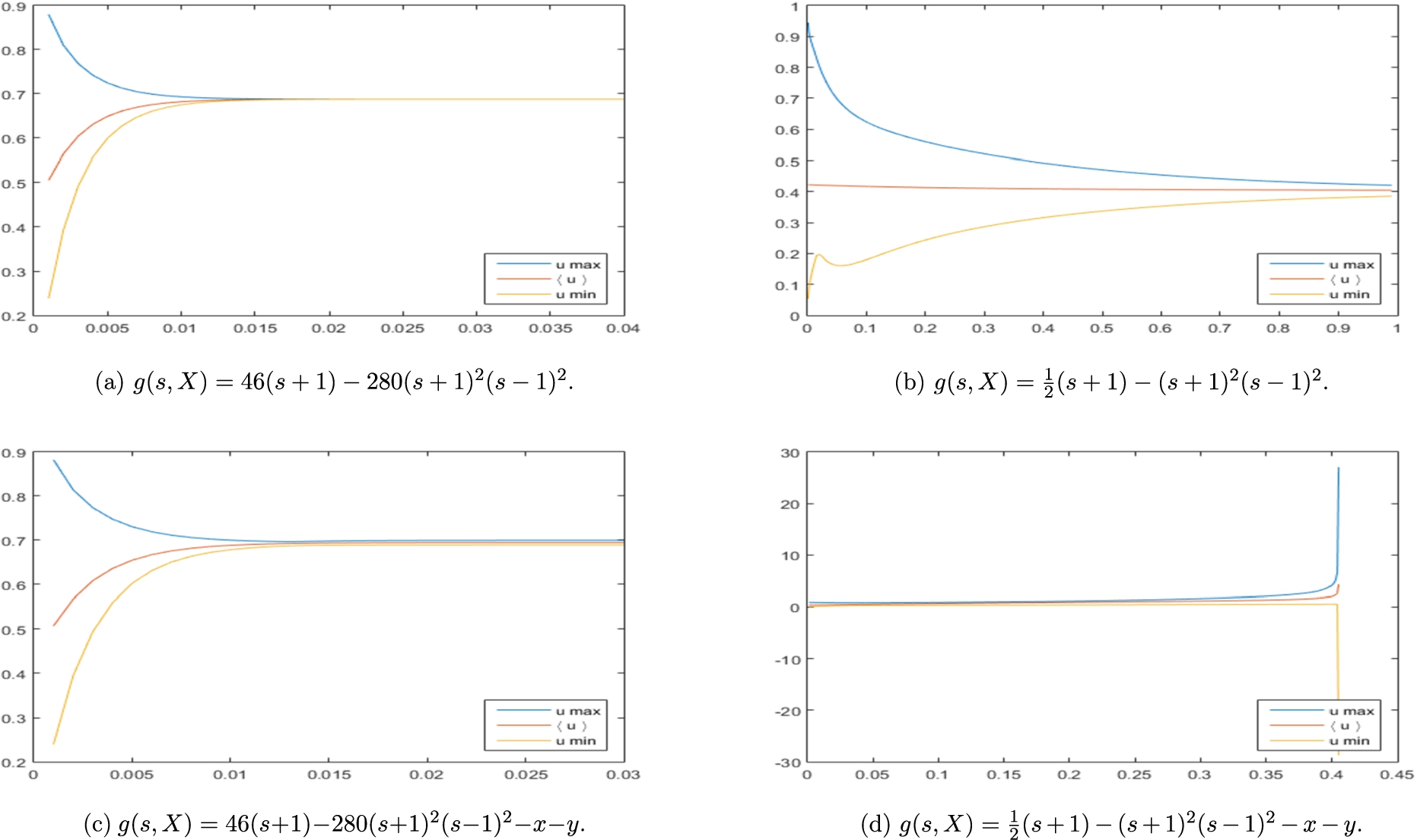
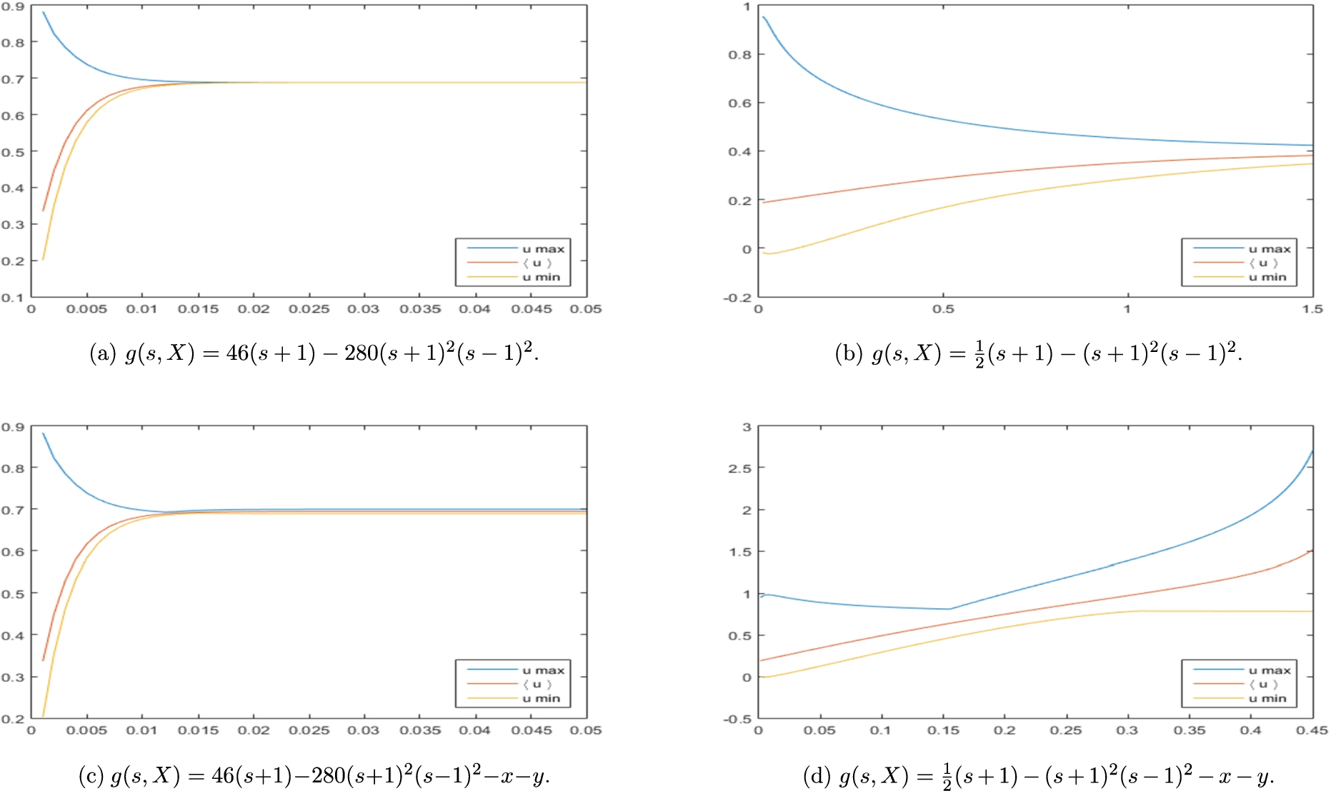
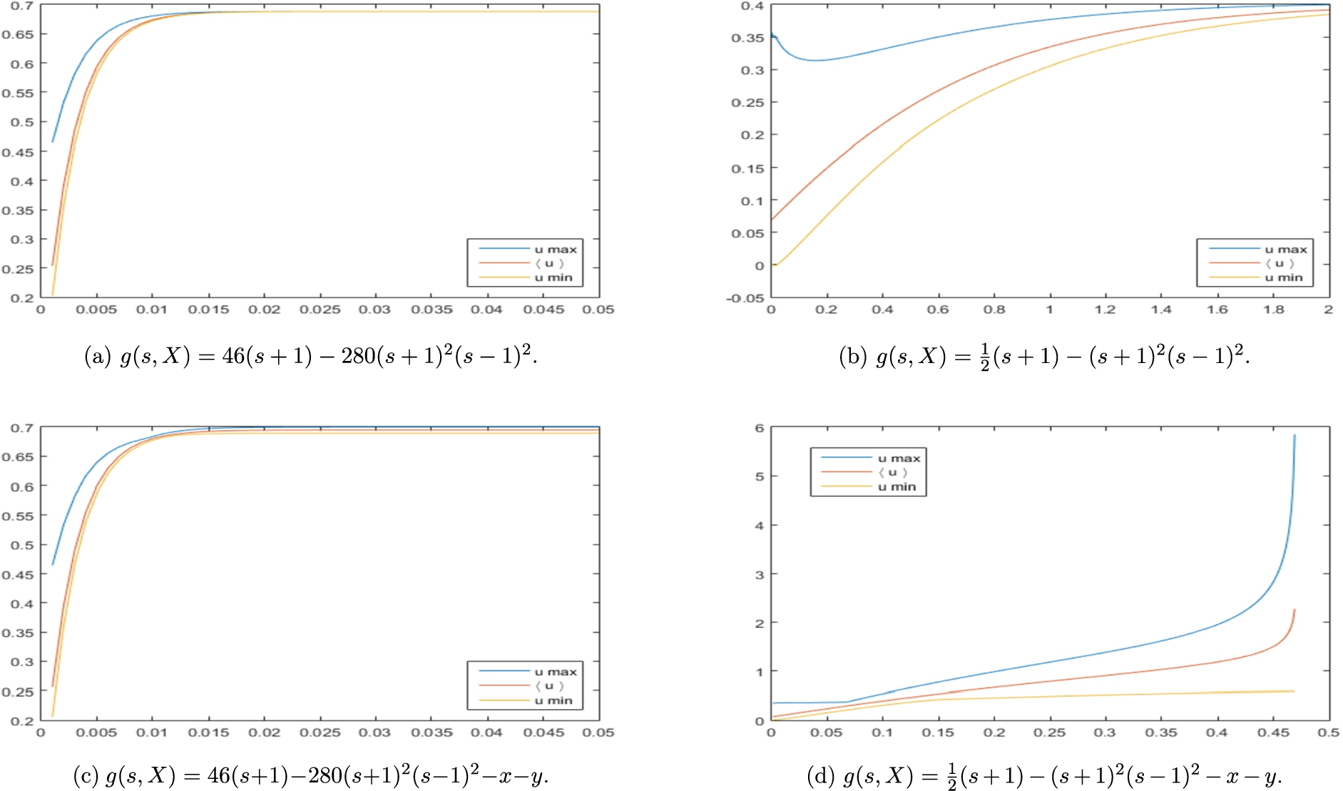
5.1. The case when $f (s) = {(s - \frac{1}{2})}^{3} - (s - \frac{1}{2})$

The figures below show the evolution of $u_{min} = {min}_{x \in Ω} u (x)$ , $u_{max} = {max}_{x \in Ω} u (x)$ and $⟨ u ⟩$ with respect to time, u being the numerical solution to (29).

In Fig. 1, we take $u_{0} (x, y) = 1 - {sin}^{2} (x + y)$ , leading to $u_{0} \in [- 1, 1]$ and $⟨ u_{0} ⟩ = 0.422572 < 1$ . Figure 2 corresponds to the initial datum $u_{0} (x, y) = \frac{cos (x - y)}{x^{6} + 1}$ , leading to $u_{0} \in [- 1, 1]$ and $⟨ u_{0} ⟩ = 0.185187 < 1$ . In Fig. 3, we take $u_{0} (x, y) = \frac{1}{5 (x^{6} + 1) (y^{5} + 0.5)}$ , leading to $u_{0} \in [- 1, 1]$ and $⟨ u_{0} ⟩ = 0.0692594 < 1$ .

Fig. 1.

$u_{0} (x, y) = 1 - {sin}^{2} (x + y)$ .

Fig. 2.

$u_{0} (x, y) = \frac{cos (x - y)}{x^{6} + 1}$ .

Fig. 3.

$u_{0} (x, y) = \frac{1}{5 (x^{6} + 1) (y^{5} + 0.5)}$ .

Figures 1a, 2a and 3a correspond to the case $λ_{1} = 92$ , $λ_{2} = 280$ and $h \equiv 0$ . The solutions remain in the biologically relevant interval $[- 1, 1]$ .

In Figs 1b, 2b and 3b, we take $λ_{1} = λ_{2} = 1$ and $h \equiv 0$ . The solutions stay in $[- 1, 1]$ .

Figures 1c, 2c and 3c correspond to the case $h (X) = x + y$ and $λ_{1} = 92$ and $λ_{2} = 280$ . The solutions stay in $[- 1, 1]$ .

In Figs 1d, 2d and 3d, we take $h (X) = x + y$ and $λ_{1} = λ_{2} = 1$ . The solutions blow up in finite time.

Table 1 provides the numerical results obtained for different initial datum with different values for $λ_{1}$ and $λ_{2}$ and changing the function h.

Table 1

Numerical results

$u_{0} (x, y)$			$1 - {sin}^{2} (x + y)$	$\frac{cos (x - y)}{x^{6} + 1}$	$\frac{1}{5 (x^{6} + 1) (y^{5} + 0.5)}$
$⟨ u_{0} ⟩$			0.422572	0.185187	0.0692594
$g (s) = \frac{λ_{1}}{2} (s + 1) - λ_{2} {(s + 1)}^{2} {(s - 1)}^{2} - h (X)$	$λ_{1} = 96$ $λ_{2} = 280$	$h \equiv 0$	No blow up	No blow up	No blow up
		$h (x, y) = x + y$	No blow up	No blow up	No blow up
		$h (x, y) = x^{2}$	No blow up	No blow up	No blow up
		$h (x, y) = x y$	No blow up	No blow up	No blow up
	$λ_{1} = 1$ $λ_{2} = 1$	$h \equiv 0$	No blow up	No blow up	No blow up
		$h (x, y) = x + y$	Blow up	Blow up	Blow up
		$h (x, y) = x^{2}$	Blow up	Blow up	Blow up
		$h (x, y) = x y$	Blow up	Blow up	Blow up

5.2. The case when

f (s) = - 2 s + \frac{1}{2} ln (\frac{1 + s}{1 - s})

The figures below show the variation of u, u being the numerical solution to (29).

Fig. 4.

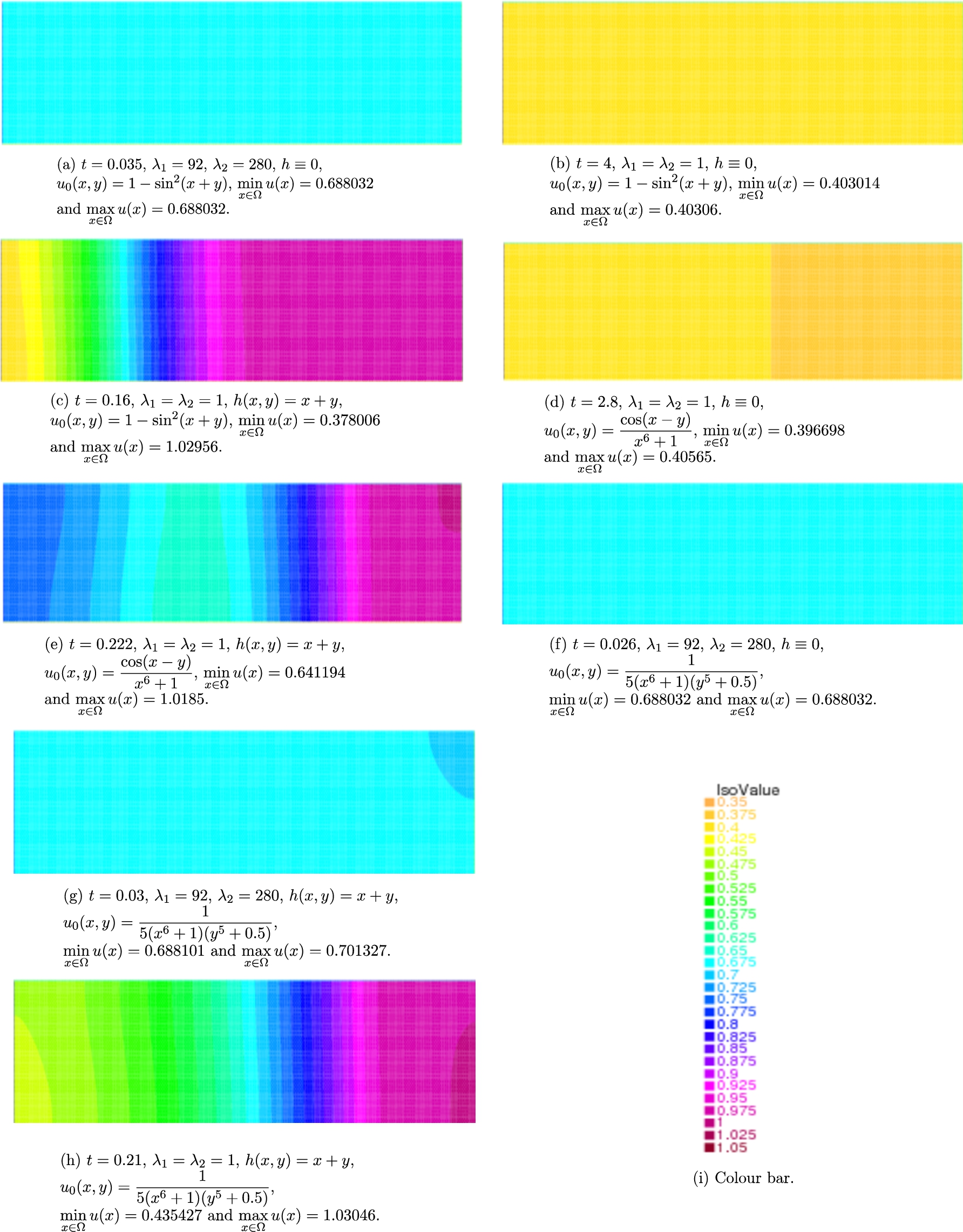
(a)–(h) Numerical solutions corresponding to different initial datum with different values for $λ_{1}$ and $λ_{2}$ and changing the function h. (i) The colour bar shows the association between colours and numerical values.

In Figs 4a, 4b and 4c, we take $u_{0} (x, y) = 1 - {sin}^{2} (x + y)$ , leading to $u_{0} \in [- 1, 1]$ and $⟨ u_{0} ⟩ = 0.422572 < 1$ . Figures 4d and 4e correspond to the initial datum $u_{0} (x, y) = \frac{cos (x - y)}{x^{6} + 1}$ , leading to $u_{0} \in [- 1, 1]$ and $⟨ u_{0} ⟩ = 0.185187 < 1$ . In Figs 4f, 4g and 4h, we take $u_{0} (x, y) = \frac{1}{5 (x^{6} + 1) (y^{5} + 0.5)}$ , leading to $u_{0} \in [- 1, 1]$ and $⟨ u_{0} ⟩ = 0.0692594 < 1$ .

Figures 4a and 4f correspond to the case $λ_{1} = 92$ , $λ_{2} = 280$ and $h \equiv 0$ . The solutions remain in the biologically relevant interval $[- 1, 1]$ .

In Figs 4b and 4d, we take $λ_{1} = λ_{2} = 1$ and $h \equiv 0$ . The solutions stay in $[- 1, 1]$ .

In Figs 4c, 4e and 4h, we take $h (X) = x + y$ and $λ_{1} = λ_{2} = 1$ . The solutions do not remain in $[- 1, 1]$ , in agreement with the theoretical results obtained in Remark 4.2 (indeed, $\frac{λ_{1}}{2} - h^{*} = - \frac{5}{2} ⩽ 0$ then $\frac{2 κ}{λ_{1}} = \frac{2}{λ_{1}} (h^{*} - \frac{λ_{1}}{2} + λ_{2}) = 7 > 1$ ).

Figure 4g corresponds to the case $h (X) = x + y$ , $λ_{1} = 92$ and $λ_{2} = 280$ . The solution stays in $[- 1, 1]$ .

Table 2 provides the numerical results obtained for different initial datum with different values for $λ_{1}$ and $λ_{2}$ and changing the function h. The results supports the theoretical results obtained in Remark 4.2. Indeed, for $λ_{1} = λ_{2} = 1$ we have $\frac{λ_{1}}{2} - h^{*} = - \frac{3}{4}$ , $- \frac{47}{6}$ , and $- \frac{5}{2} ⩽ 0$ for $h (X) = x y$ , $x^{2}$ , and $x + y$ , respectively, then $\frac{2 κ}{λ_{1}} = \frac{2}{λ_{1}} (h^{*} - \frac{λ_{1}}{2} + λ_{2}) = \frac{7}{2}$ , $\frac{53}{3}$ , and 7, respectively, i.e., $\frac{2 κ}{λ_{1}} > 1$ .

Table 2

Numerical results

$u_{0} (x, y)$			$1 - {sin}^{2} (x + y)$	$\frac{cos (x - y)}{x^{6} + 1}$	$\frac{1}{5 (x^{6} + 1) (y^{5} + 0.5)}$
$⟨ u_{0} ⟩$			0.422572	0.185187	0.0692594
$g (s) = \frac{λ_{1}}{2} (s + 1) - λ_{2} {(s + 1)}^{2} \times {(s - 1)}^{2} - h (X)$	$λ_{1} = 96$ $λ_{2} = 280$	$h \equiv 0$	Stay in $[- 1, 1]$	Stay in $[- 1, 1]$	Stay in $[- 1, 1]$
		$h (x, y) = x + y$	Stay in $[- 1, 1]$	Stay in $[- 1, 1]$	Stay in $[- 1, 1]$
		$h (x, y) = x^{2}$	Stay in $[- 1, 1]$	Stay in $[- 1, 1]$	Stay in $[- 1, 1]$
		$h (x, y) = x y$	Stay in $[- 1, 1]$	Stay in $[- 1, 1]$	Stay in $[- 1, 1]$
		$h (x, y) = y$	Stay in $[- 1, 1]$	Stay in $[- 1, 1]$	Stay in $[- 1, 1]$
	$λ_{1} = 1$ $λ_{2} = 1$	$h \equiv 0$	Stay in $[- 1, 1]$	Stay in $[- 1, 1]$	Stay in $[- 1, 1]$
		$h (x, y) = x + y$	Do not stay in $[- 1, 1]$	Do not stay in $[- 1, 1]$	Do not stay in $[- 1, 1]$
		$h (x, y) = x^{2}$	Do not stay in $[- 1, 1]$	Do not stay in $[- 1, 1]$	Do not stay in $[- 1, 1]$
		$h (x, y) = x y$	Do not stay in $[- 1, 1]$	Do not stay in $[- 1, 1]$	Do not stay in $[- 1, 1]$
		$h (x, y) = y$	Stay in $[- 1, 1]$	Stay in $[- 1, 1]$	Stay in $[- 1, 1]$

6. Conclusion

In this work, we provide existence results for a Cahn–Hilliard equation in view of applications in biology, more precisely, to model tumor growth and wound healing. We consider the equation endowed with Neumann boundary conditions and take $\begin{matrix} g (s) = \frac{λ_{1}}{2} (1 + s) - λ_{2} {(1 + s)}^{2} {(1 - s)}^{2}, λ_{1}, λ_{2} > 0 . \end{matrix}$ First, we consider a regular nonlinear term. The existence of local (in time) solution is shown using a Galerkin method, a priori estimates and compactness method. We were also able to prove the continuous dependence on initial data for the solution in $H^{- 1} (Ω)$ . Then, we consider a logarithmic nonlinear term. We prove the existence of a local (in time) biologically relevant solution to the problem. In this case, we have not been able to prove the uniqueness of solutions. We then prove that, if $λ_{2} ⩽ λ_{1}$ then the solution is global (in time). We finally give some numerical simulations which confirm these results.

References

A.C.

Aristotelous,

O.A.

Karakashian and

S.M.

Wise Adaptive, Second-Order in Time, Primitive-Variable Discontinuous Galerkin Schemes for a Cahn–Hilliard Equation with a Mass Source, IMA Journal of Numerical Analysis (2015), 1167–1198. doi:10.1093/imanum/dru035.

A.L.

Bertozzi,

Esedoglu and

Gillette, Analysis of a Two-Scale Cahn–Hilliard Model for Binary Image Inpainting, Multiscale Modeling and Simulation (2007), 913–936. doi:10.1137/060660631.

A.L.

Bertozzi,

Esedoglu and

Gillette, Inpainting of binary images using the Cahn–Hilliard equation, IEEE Transactions on Image Processing (2007), 285–291. doi:10.1109/TIP.2006.887728.

J.W.

Cahn, On spinodal decomposition, Acta Metallurgica (1961), 795–801. doi:10.1016/0001-6160(61)90182-1.

J.W.

Cahn and

J.E.

Hilliard, Free energy of a nonuniform system. I. Interfacial free energy, The Journal of Chemical Physics (1958), 258–267. doi:10.1063/1.1744102.

Capuzzo Dolcetta,

Finzi Vita and

March, Area preserving curve shortening flows: From phase transitions to image processing, Interfaces and Free Boundaries (2002), 325–343. doi:10.4171/IFB/64.

Cherfils,

Miranville and

Zelik, On a generalized Cahn–Hilliard equation with biological applications, Discrete and Continuous Dynamical Systems (2014), 2013–2026. doi:10.3934/dcdsb.2014.19.2013.

Debussche and

Dettori, On the Cahn–Hilliard equation with a logarithmic free energy, Nonlinear Analysis (1995), 1491–1514. doi:10.1016/0362-546X(94)00205-V.

S.C.

Donald and

J.D.

Murray, A generalized diffusion model for growth and dispersion in a population, Journal of Mathematical Biology (1981), 237–248.

10.

C.M.

Elliott and

Garcke, On the Cahn–Hilliard Equation with Degenerate Mobility, SIAM Journal on Mathematical Analysis (1996), 404–423. doi:10.1137/S0036141094267662.

11.

Fakih, A Cahn–Hilliard equation with a proliferation term for biological and chemical applications, Asymptotic Analysis (2015), 71–104. doi:10.3233/ASY-151306.

12.

Fakih, Asymptotic behavior of a generalized Cahn–Hilliard equation with a mass source, Applicable Analysis (2017), 324–348. doi:10.1080/00036811.2015.1135241.

13.

Freefem++ is freely available at: http://www.freefem.org/ff.

14.

Frigeri and

Grasselli, Nonlocal Cahn–Hilliard–Navier–Stokes systems with singular potentials, Dynamics of PDE (2012), 273–304.

15.

Hassan Farshbaf-Shaker and

Heinemann, A phase field approach for optimal boundary control of damage processes in two-dimensional viscoelastic media, Mathematical Models and Methods in Applied Sciences (2015), 2749–2793.

16.

Hilhorst,

Johannes,

Nam Nguyen and

van Der Zee Kristoffer, Formal asymptotic limit of a diffuse-interface tumor-growth model, Mathematical Models and Methods in Applied Sciences (2015), 1011–1043. doi:10.1142/S0218202515500268.

17.

Khain and

L.M.

Sander, A generalized Cahn–Hilliard equation for biological applications, Physical review E (2008).

18.

Klapper and

Dockery, Role of cohesion in the material description of biofilms, Physical review E (2006).

19.

J.-L.

Lions, Quelques méthodes de résolution des problèmes aux limites non linéaires, Dunod, 1969.

20.

Q.-X.

Liu,

Doelman,

Rottschafer,

de Jager,

P.M.J.

Herman,

Rietkerk and

van de Koppel, Phase separation explains a new class of self-organized spatial patterns in ecological systems, in: Proceedings of the National Academy of Sciences, 2013, pp. 11905–11910.

21.

Miranville, Asymptotic behavior of the Cahn–Hilliard-Oono equation, Journal of Applied Analysis and Computation (2011), 523–536. doi:10.11948/2011036.

22.

Miranville, Asymptotic behaviour of a generalized Cahn–Hilliard equation with a proliferation term, Applicable Analysis (2013), 1308–1321. doi:10.1080/00036811.2012.671301.

23.

Miranville, The Cahn–Hilliard equation and some of its variants, AIMS Mathematics (2017), 479–544. doi:10.3934/Math.2017.2.479.

24.

Miranville, Existence of Solutions to a Cahn–Hilliard Type Equation with a Logarithmic Nonlinear Term, Mediterranean Journal of Mathematics (2019), 1–18.

25.

Oono and

Puri, Computationally efficient modeling of ordering of quenched phases, Physical review letters (1987), 836–839. doi:10.1103/PhysRevLett.58.836.

26.

Oron,

S.H.

Davis and

S.G.

Bankoff, Long-scale evolution of thin liquid films, Review of Modern Physics (1997), 931–980. doi:10.1103/RevModPhys.69.931.

27.

Thiele and

Knobloch, Thin liquid films on a slightly inclined heated plate, Physica D Nonlinear Phenomena (2004), 213–248. doi:10.1016/j.physd.2003.09.048.

28.

Tremaine, On the origin of irregular structure in Saturn’s rings, The Astronomical Journal (2003), 894–901. doi:10.1086/345963.

29.

Verdasca,

Borckmans and

Dewel, Chemically frozen phase separation in an adsorbed layer, Physical review E (1995), 4616–4619. doi:10.1103/PhysRevE.52.R4616.

30.

Villain-Guillot, Phases modulées et dynamique de Cahn–Hilliard, PhD thesis, Université Bordeaux I, 2010.

31.

Zhou and

M.Y.

Wang, Multimaterial structural topology optimization with a generalized Cahn–Hilliard model of multiphase transition, Structural and Multidisciplinary Optimization (2007), 89–111.

Existence of solution to a Cahn–Hilliard equation