Homogenization of a class of singular elliptic problems in two-component domains

Abstract

This paper deals with the homogenization of a quasilinear elliptic problem having a singular lower order term and posed in a two-component domain with an ε-periodic imperfect interface. We prescribe a Dirichlet condition on the exterior boundary, while we assume that the continuous heat flux is proportional to the jump of the solution on the interface via a function of order $ε^{γ}$ .

We prove an homogenization result for $- 1 < γ < 1$ by means of the periodic unfolding method (see SIAM J. Math. Anal. 40 (2008) 1585–1620 and The Periodic Unfolding Method (2018) Springer), adapted to two-component domains in (J. Math. Sci. 176 (2011) 891–927).

One of the main tools in the homogenization process is a convergence result for a suitable auxiliary linear problem, associated with the weak limit of the sequence ${u^{ε}}$ of the solutions, as $ε \to 0$ . More precisely, our result shows that the gradient of $u^{ε}$ behaves like that of the solution of the auxiliary problem, which allows us to pass to the limit in the quasilinear term, and to study the singular term near its singularity, via an accurate a priori estimate.

Keywords

Two-component domains Homogenization Periodic Unfolding Method Quasilinear elliptic equations Singular equations

1. Introduction

In this paper we study the asymptotic behavior of a class of quasilinear elliptic problems presenting singular lower order terms and posed in two-component domains.

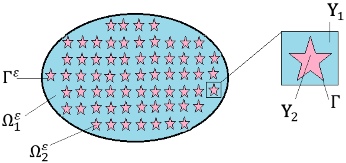
More precisely, the two-component domain Ω is a bounded open subset of $R^{N}$ which is the union of two disjoint open subsets, $Ω_{1}^{ε}$ and $Ω_{1}^{ε}$ , and their common boundary $Γ^{ε}$ . The disconnected component $Ω_{2}^{ε}$ is the union of the ε-periodic translated sets of $ε Y_{2}$ , where $Y_{2}$ is well contained in the reference cell Y and $Γ = \partial Y_{2}$ . The connected component $Ω_{1}^{ε}$ is obtained by removing from Ω the closure of $Ω_{2}^{ε}$ such that the interface $Γ^{ε} = \partial Ω_{2}^{ε}$ .

We deal with the homogenization, as ε goes to zero, of the following problem: $\begin{matrix} \{\begin{matrix} - div (A^{ε} (x, u^{ε}) \nabla u^{ε}) = f ζ (u^{ε}) & in Ω ∖ Γ^{ε}, \\ u_{1}^{ε} = 0 & on \partial Ω, \\ (A^{ε} (x, u_{1}^{ε}) \nabla u_{1}^{ε}) ν^{ε} = (A^{ε} (x, u_{2}^{ε}) \nabla u_{2}^{ε}) ν^{ε} & on Γ^{ε}, \\ (A^{ε} (x, u_{1}^{ε}) \nabla u_{1}^{ε}) ν^{ε} = - ε^{γ} h^{ε} (u_{1}^{ε} - u_{2}^{ε}) & on Γ^{ε}, \end{matrix} \end{matrix}$ where $ν^{ε}$ is the unit external normal vector to $Ω_{1}^{ε}$ . We prescribe a Dirichlet condition on the exterior boundary, while we assume that the continuous heat flux is proportional to the jump of the solution on the interface by means of a function of order $ε^{γ}$ .

The quasilinear diffusion matrix field is defined by $A^{ε} (x, t) = A (\frac{x}{ε}, t)$ , where the matrix field A is uniformly elliptic, bounded, periodic in the first variable and Carathéodory. The nonlinear real function $ζ (s)$ is nonnegative and singular at $s = 0$ , while f is a nonnegative datum whose summability depends on the growth of ζ near its singularity. Concerning the boundary condition, $h^{ε} (x) = h (\frac{x}{ε})$ where h is assumed to be a periodic, nonnegative and bounded function, and $γ \in] - 1, 1 [$ .

This problem describes the stationary heat diffusion in a two-component composite with an ε-periodic imperfect interface. In particular, quasilinear diffusion terms describe the behavior of materials like glass or wood, in which the heat diffusion depends on the range of the temperature (see for instance [6]). We refer to [20, Section 3] for more details about source terms depending on the solution itself and becoming infinite when the solutions vanish. These kind of source terms can model, for instance, electrical conductors where each point becomes a source of heat as a current flows inside. The boundary condition on $Γ^{ε}$ models a jump of the solution through a rough interface and we refer to [9] for a physical justification of this model (see also [29]).

In view of a counterexample suggested by H.C. Hummel in [28], one cannot expect bounded a priori estimates for the solution when $γ > 1$ . For this case we refer to [23] where different a priori estimates needed. As for our problem, existence and uniqueness results has been proved in [25,26] for $γ ⩽ 1$ .

Here we prove an homogenization result for $γ \in] - 1, 1 [$ by means of the periodic unfolding method. This method was originally introduced by D. Cioranescu, A. Damlamian and G. Griso in [13] and [14] for fixed domains and extended to perforated ones in [16] and [17]. Then, it has been adapted to two-component domains by P. Donato, K.H. Le Nguyen and R. Tardieu in [22] (see also [21]).

This work has been partially inspired by the works [20] and [24]. Let us point out the main differences with respect to them and the additional difficulties. In [20] the authors treat the same singularity when A is linear and in a different geometrical framework where the domain has two connected components separated by an oscillating interface. This interface tends to a flat one, so that the integral on $Γ^{ε}$ goes to the one on Γ, roughly speaking. But here $Γ^{ε}$ is the union of disconnected sets (of order $\frac{1}{ε}$ ) so that its measures goes to inifnity, whence the integral on $Γ^{ε}$ needs particular care.

Let us mention that in [24] the authors consider the same singular problem with A quasilinear but posed in a periodically perforated domain. Here the holes are replaced by a second material so that we have to treat in addition all the integrals on the second component and the boundary term with jump.

In Section 2 we present the setting of the problem and we state the main results.

In Section 3 we give a short presentation of the periodic unfolding method, adapted to two-component domains.

In Section 4 we prove two a priori estimates uniform with respect to ε and we give an estimate of the integral of the singular term close to the singular set ${u^{ε} = 0}$ , in terms of the quasilinear one (cf. Proposition 4.3).

In Section 5 we prove a crucial convergence result, Theorem 5.4. It is one of the main tools when proving our homogenization result and it shows that the gradient of $u^{ε}$ is equivalent to the gradient of the solution of a suitable auxiliary linear problem, associated with a weak cluster point of the sequence ${u^{ε}}$ , as $ε \to 0$ . This idea was originally introduced in [4] (see also [5]) where some nonlinear problems with quadratic growth are considered. We refer to [10] and [22] for the study of the auxiliary problem, while for the proof of the convergence result we adapt some techniques from [20] and [24].

Section 6 is devoted to the proofs of Proposition 2.5 and the homogenization theorem. For these results Theorem 5.4 plays an important rule not only in the study of the quasilinear term but also in that of the singular one. Actually, as done in [20] and [24], we split the integral of the singular term into the sum of two integrals: one on the set where the solution is close to the singularity and one where is it far from it, which results not singular. Near the singularity, making use of the estimate given in Proposition 4.3, we shift the study of the singular term to that of the quasilinear one, for which we can use Theorem 5.4.

Finally, let us point out that the homogenization result we prove here shows that the conductivity of the first material is the same obtained when there is no material occupying $Ω_{2}^{ε}$ . On the other hand, since in the limit problem it appears f instead of $θ_{1} f$ (being $θ_{1}$ the proportion of the material occupying $Ω_{1}^{ε}$ ), one has anyway to take into account even the source term in the second component.

The first paper on this subject is due to [3] for the linear (nonsingular) case by multiple scale method. In [23] and [29] the authors also studied the linear case by using the Tartar method. For similar homogenization elliptic problems we refer to [8,20,24,28] and [30]. In [21,22] the authors study the linear case in presence of linear and nonlinear boundary conditions, respectively.

2. Setting of the problem and main results

Throughout the paper, we use the same notation as in [21,22] for the periodic unfolding method in two-component domains.

The domain. For $N \in N$ , $N ⩾ 2$ , let Ω be a bounded open set in $R^{N}$ with a Lipschitz-continuous boundary $\partial Ω$ . Also let $Y ≐ \prod_{i = 1}^{N} [0, l_{i} [$ be a reference cell, with $l_{i} > 0$ , $i = 1, \dots, N$ . We suppose that $Y_{1}$ and $Y_{2}$ are two disjoint connected open subsets of Y such that $Y_{2} \neq \emptyset$ , $\overline{Y_{2}} \subset Y$ and $Y = Y_{1} \cup \overline{Y_{2}}$ , with a common boundary $Γ = \partial Y_{2}$ Lipschitz-continuous.

Let ${ε}_{ε > 0}$ be a positive parameter taking values in a sequence converging to zero and set:

for any $k \in Z^{N}$ , $k_{l} = (k_{1} l_{1}, \dots, k_{N} l_{N})$ and $\begin{matrix} Y^{k} = k_{l} + Y, Y_{i}^{k} = k_{l} + Y_{i}, i = 1, 2, \end{matrix}$

$K_{ε} = {k \in Z^{N} | ε \overline{Y_{2}^{k}} \subset Ω}$ and $\begin{matrix} Ω_{2}^{ε} = ⋃_{k \in K_{ε}} ε Y_{2}^{k}, Ω_{1}^{ε} = Ω ∖ \overline{Ω_{2}^{ε}}, Γ^{ε} = \partial Ω_{2}^{ε} . \end{matrix}$ By construction, Ω results the union of the two disjoint components and their common boundary, i.e. $Ω = Ω_{1}^{ε} \cup Ω_{2}^{ε} \cup Γ^{ε}$ (see Fig. 1).

Also we introduce the following sets: $\begin{matrix} {\hat{K}}_{ε} = {k \in Z^{N} | ε Y^{k} \subset Ω}, {\hat{Ω}}_{ε} = interior {⋃_{k \in {\hat{K}}_{ε}} ε (k_{l} + \overline{Y})}, Λ_{ε} = Ω ∖ {\hat{Ω}}_{ε}, \end{matrix}$ and $\begin{matrix} {\hat{Ω}}_{i}^{ε} = ⋃_{k \in {\hat{K}}_{ε}} ε Y_{i}^{k}, Λ_{i}^{ε} = Ω_{i}^{ε} ∖ {\hat{Ω}}_{i}^{ε}, i = 1, 2, {\hat{Γ}}^{ε} = \partial {\hat{Ω}}_{2}^{ε} . \end{matrix}$ Also, $\begin{matrix} (2.1) & there exists ε_{0} > 0 such that \forall ε ⩽ ε_{0}, Λ_{2}^{ε} = \emptyset . \end{matrix}$ Let us note that here, for the sake of simplicity, we do not allow the second component to meet the boundary of the domain and also we suppose $Y_{2}$ connected. Actually the cases where the holes meet the boundary of Ω and $Y_{2}$ has a finite number of connected components can be treated as done in [21] and [22], respectively.

Fig. 1.

The two-component domain Ω and the reference cell Y.

In the sequel we denote by

$M_{ω} (v) ≐ \frac{1}{| ω |} \int_{ω} v d x$ the average of any function $v \in L^{1} (ω)$ , for any open set ω of $R^{N}$ ,

$χ_{ω}$ the characteristic function of any open set ω of $R^{N}$ ,

∼ the zero extension to the whole of Ω of functions defined on $Ω_{1}^{ε}$ or $Ω_{2}^{ε}$ ,

$θ_{i} ≐ \frac{| Y_{i} |}{| Y |}$ , $i = 1, 2$ ,

c different positive constants independent on ε,

$M (α, β, Y)$ the set of matrix fields $A = {(a_{i, j})}_{1 ⩽ i, j ⩽ N} \in {(L^{\infty} (Y))}^{N \times N}$ such that $\begin{matrix} (A (x) λ, λ) ⩾ α | λ |^{2} and | A (x) λ | ⩽ β | λ |, \forall λ \in R^{N} and a.e. in Y, \end{matrix}$ with $α, β \in R$ , $0 < α ⩽ β$ ,

${e_{1}, \dots, e_{N}}$ the canonical basis of $R^{N}$ ,

$v_{i} = v_{| Ω_{i}^{ε}}$ the restriction to $Ω_{i}^{ε}$ of functions v defined in Ω, $i = 1, 2$ .

Moreover let us recall the classical decomposition for every real function v

\begin{matrix} (2.2) & v = v^{+} - v^{-}, v^{+} ≐ max {v, 0} and v^{-} ≐ - min {v, 0} a.e. in Ω, \end{matrix}

where

v^{+}

and

v^{-}

are both nonnegative. In particular, one has

\begin{matrix} (2.3) & \begin{matrix} (v_{1} - v_{2}) (v_{1}^{-} - v_{2}^{-}) & = (v_{1}^{+} - v_{2}^{+}) (v_{1}^{-} - v_{2}^{-}) - {(v_{1}^{-} - v_{2}^{-})}^{2} \\ = - v_{1}^{+} v_{2}^{-} - v_{2}^{+} v_{1}^{-} - {(v_{1}^{-} - v_{2}^{-})}^{2} ⩽ 0 . \end{matrix} \end{matrix}

The problem. The aim of the paper is to study the asymptotic behavior, as ε goes to zero, of the following problem: $\begin{matrix} (2.4) & \{\begin{matrix} - div (A^{ε} (x, u^{ε}) \nabla u^{ε}) = f ζ (u^{ε}) & in Ω ∖ Γ^{ε}, \\ u_{1}^{ε} = 0 & on \partial Ω, \\ (A^{ε} (x, u_{1}^{ε}) \nabla u_{1}^{ε}) ν^{ε} = (A^{ε} (x, u_{2}^{ε}) \nabla u_{2}^{ε}) ν^{ε} & on Γ^{ε}, \\ (A^{ε} (x, u_{1}^{ε}) \nabla u_{1}^{ε}) ν^{ε} = - ε^{γ} h^{ε} (u_{1}^{ε} - u_{2}^{ε}) & on Γ^{ε}, \end{matrix} \end{matrix}$ where $ν^{ε}$ is the unit external normal vector to $Ω_{1}^{ε}$ , and we prescribe a Dirichlet condition on the exterior boundary and a jump of the solution on the interface $Γ^{ε}$ , in the case $γ \in] - 1, 1 [$ .

Assumptions on the data.

The real $N \times N$ matrix field $A : (y, t) \in Y \times R \mapsto A (y, t) = {(a_{i, j} (y, t))}_{i, j = 1, \dots, N} \in R^{N^{2}}$ satisfies the following conditions: $\begin{matrix} \{\begin{matrix} i) A is a Carathéodory function s.t. \\ A (\cdot, t) is Y -periodic and in M (α, β, Y), for every t \in R; \\ ii) there exists a real function ω : R \to R satisfying the following conditions: \\ - ω is continuous and non decreasing, with ω (t) > 0 \forall t > 0, \\ - | A (y, t_{1}) - A (y, t_{2}) | ⩽ ω (| t_{1} - t_{2} |) for a.e. y \in Y, \forall t_{1} \neq t_{2}, \\ - \forall s > 0, {lim}_{y \to 0^{+}} \int_{y}^{s} \frac{d t}{ω (t)} = + \infty . \end{matrix} \end{matrix}$

The functions ζ and f verify $\begin{array}{l} \{\begin{matrix} i) ζ : [0, + \infty [\to [0, + \infty] is a function such that \\ ζ \in C^{0} ([0, + \infty [), 0 ⩽ ζ (s) ⩽ \frac{1}{s^{k}} for every s \in] 0, + \infty [, with 0 < k ⩽ 1; \\ ii) ζ is non increasing; \end{matrix} \\ iii) f ⩾ 0 a.e. in Ω, f ≢ 0, with f \in L^{l} (Ω), for l ⩾ \frac{2}{1 + k} (⩾ 1) . \end{array}$

$- 1 < γ < 1$ , and h is a Y-periodic function in $L^{\infty} (Γ)$ such that $\begin{matrix} there exists h_{0} \in R : 0 < h_{0} < h (y) a.e. on Γ . \end{matrix}$

Under the above assumptions we set, for every $t \in R$ , $\begin{matrix} (2.5) & A^{ε} (x, t) ≐ A (\frac{x}{ε}, t) for a.e. x \in Ω, h^{ε} (x) ≐ h (\frac{x}{ε}) for a.e. x \in Γ^{ε} . \end{matrix}$

The functional framework. We now introduce the functional spaces used in the literature to handle (2.4)-type problems.

Let $V^{ε} ≐ {v \in H^{1} (Ω_{1}^{ε}) | v = 0 on \partial Ω}$ endowed with the norm $\begin{matrix} ‖ v ‖_{V^{ε}} = ‖ \nabla v ‖_{L^{2} (Ω_{1}^{ε})} . \end{matrix}$

Remark 2.1.

It is known (see for instance [18, Lemma 1], [19]) that a Poincaré inequality in $V^{ε}$ holds with a constant $c_{P}$ independent on ε, that is $\begin{matrix} (2.6) & ‖ v ‖_{L^{2} (Ω_{1}^{ε})} ⩽ c_{P} ‖ \nabla v ‖_{L^{2} (Ω_{1}^{ε})} \forall v \in V^{ε} . \end{matrix}$ Consequently, the norm in $V^{ε}$ is equivalent to that in $H^{1} (Ω_{1}^{ε})$ via a constant independent on ε.

For every $γ \in R$ , let $H_{γ}^{ε}$ be the space defined by $\begin{matrix} H_{γ}^{ε} ≐ {v \in L^{2} (Ω) | v_{1} \in V^{ε}, v_{2} \in H^{1} (Ω_{2}^{ε})}, \end{matrix}$ which, after the identification $\nabla v : = \tilde{\nabla v_{1}} + \tilde{\nabla v_{2}}$ , is equipped by the norm $\begin{matrix} ‖ v ‖_{H_{γ}^{ε}}^{2} ≐ ‖ \nabla v ‖_{L^{2} (Ω ∖ Γ^{ε})}^{2} + ε^{γ} ‖ v_{1} - v_{2} ‖_{L^{2} (Γ^{ε})}^{2} . \end{matrix}$

Proposition 2.2 ([22,29]).

Let $γ ⩽ 1$ . There exist some positive constants $c_{1}$ , $c_{2}$ and C, independent of ε, such that $\begin{matrix} \forall v \in H_{γ}^{ε}, c_{1} ‖ v ‖_{V^{ε} \times H^{1} (Ω_{2}^{ε})}^{2} ⩽ ‖ v ‖_{H_{γ}^{ε}}^{2} ⩽ c_{2} (1 + ε^{γ - 1}) ‖ v ‖_{V^{ε} \times H^{1} (Ω_{2}^{ε})}^{2} . \end{matrix}$ In addition, if $v^{ε} = (v_{1}^{ε}, v_{2}^{ε})$ is a bounded sequence in $H_{γ}^{ε}$ , then $\begin{array}{l} {‖ v_{1}^{ε} ‖}_{H^{1} (Ω_{1}^{ε})} ⩽ C, \\ {‖ v_{2}^{ε} ‖}_{H^{1} (Ω_{2}^{ε})} ⩽ C, \\ {‖ v_{1}^{ε} - v_{2}^{ε} ‖}_{L^{2} (Γ^{ε})} ⩽ C ε^{- \frac{γ}{2}} . \end{array}$

The variational formulation associated with problem (2.4) reads $\begin{matrix} (2.7) & \{\begin{matrix} Find u^{ε} \in H_{γ}^{ε} such that u^{ε} > 0 a.e. in Ω, \\ \int_{Ω} f ζ (u^{ε}) φ d x < + \infty, and \\ \int_{Ω ∖ Γ^{ε}} A^{ε} (x, u^{ε}) \nabla u^{ε} \nabla φ d x + \int_{Γ^{ε}} ε^{γ} h^{ε} (u_{1}^{ε} - u_{2}^{ε}) (φ_{1} - φ_{2}) d σ \\ = \int_{Ω} f ζ (u^{ε}) φ d x, \forall φ \in H_{γ}^{ε} . \end{matrix} \end{matrix}$ In [25,26] it is proved that, under assumptions H₁)–H₃), problem (2.7) admits a unique solution.

Let us introduce here the homogenized matrix $A^{0} (t)$ , $t \in R$ , corresponding to our case $γ \in] - 1, 1 [$ . It is defined by $\begin{matrix} (2.8) & A^{0} (t) λ ≐ \frac{1}{| Y |} \int_{Y_{1}} A (y, t) (λ - \nabla_{y} χ_{λ} (y, t)) d y \forall λ \in R^{N}, \end{matrix}$ where, for every $λ \in R^{N}$ , $χ_{λ} (\cdot, t) \in H^{1} (Y_{1})$ are unique solutions of the cell problems $\begin{matrix} (2.9) & \{\begin{matrix} - div (A (\cdot, t) \nabla_{y} χ_{λ} (\cdot, t) = - div (A (\cdot, t) λ) & in Y_{1}, \\ A (\cdot, t) (λ - \nabla_{y} χ_{λ} (\cdot, t)) ν_{1} = 0 & on Γ, \\ χ_{λ} (\cdot, t) Y-periodic and M_{Y_{1}} (χ_{λ}) = 0 . \end{matrix} \end{matrix}$ The homogenized matrix $A^{0}$ is actually the one obtained in the framework of perforated domains. It has been originally introduced in [18] for linear problems with Neumann conditions in perforated domain, successively extended to quasilinear ones in [1] and [2].

We recall (see [7] and [18]) that the matrix $A^{0}$ satisfies the following properties: $\begin{matrix} (2.10) & \begin{array}{l} i) A^{0} is continuous and A^{0} (t) \in M (α, \frac{β^{2}}{α}, Ω) for every t \in R; \\ ii) there exists a positive constant C, depending only on α, β, Y and T s.t. \\ | A^{0} (t_{1}) - A^{0} (t_{2}) | ⩽ C ω (| t_{1} - t_{2} |) \\ for every t_{1}, t_{2} \in R, with t_{1} \neq t_{2}, where ω {is the function given in H}_{1}) . \end{array} \end{matrix}$

Remark 2.3.
Observe that assumptions H₁)_ii and H₂)_ii are only needed for the uniqueness of the solution of problem (2.7). If they do not hold true, the homogenized problem is still the same but all the convergences remain valid only for a subsequence.

The main results. We now state the main results of this work, which will be proved in Section 6.
Theorem 2.4.
Under assumptions H ₁ )–H ₃ ), let $u^{ε} \in H_{γ}^{ε}$ be the unique solution of problem ( 2.7 ). Then, there exist a subsequence (still denoted by ε), $u_{1} \in H_{0}^{1} (Ω)$ , ${\hat{u}}_{1} \in L^{2} (Ω, H_{per}^{1} (Y_{1}))$ with $M_{Γ} ({\hat{u}}_{1}) = 0$ for almost every $x \in Ω$ and ${\overline{u}}_{2} \in L^{2} (Ω, H^{1} (Y_{2}))$ with $M_{Γ} ({\overline{u}}_{2}) = 0$ for almost every $x \in Ω$ such that $\begin{matrix} (2.11) & \{\begin{matrix} i) T_{i}^{ε} (u_{i}^{ε}) \to u_{1} & strongly in L^{2} (Ω, H^{1} (Y_{i})), i = 1, 2, \\ ii) T^{ε} (ζ (u^{ε})) \to ζ (u_{1}) & a.e. in Ω \times Y, \\ iii) \tilde{u_{1}^{ε}} ⇀ θ_{1} u_{1} & weakly in L^{2} (Ω), \\ iv) T_{1}^{ε} (\nabla u_{1}^{ε}) ⇀ \nabla u_{1} + \nabla_{y} {\hat{u}}_{1} & weakly in L^{2} (Ω \times Y_{1}) \\ v) T_{2}^{ε} (\nabla u_{2}^{ε}) ⇀ \nabla_{y} {\overline{u}}_{2} & weakly in L^{2} (Ω \times Y_{2}), \end{matrix} \end{matrix}$ and $\begin{matrix} (2.12) & u_{1} ⩾ 0 a.e. in Ω and \int_{Ω} f ζ (u_{1}) φ d x < + \infty, \forall φ \in H_{0}^{1} (Ω) . \end{matrix}$ Moreover, the pair $(u_{1}, {\hat{u}}_{1})$ is the unique solution of the unfolded limit equation $\begin{matrix} (2.13) & \{\begin{matrix} \forall φ \in H_{0}^{1} (Ω) and \forall ψ \in L^{2} (Ω; H_{per}^{1} (Y_{1})) \\ \int_{Ω \times Y_{1}} A (y, u_{1}) (\nabla u_{1} + \nabla_{y} {\hat{u}}_{1}) (\nabla φ + \nabla_{y} ψ) d x d y = | Y | \int_{Ω} f ζ (u_{1}) φ d x . \end{matrix} \end{matrix}$
Proposition 2.5.
Under assumptions H ₁ )–H ₃ ), let $(u_{1}, {\hat{u}}_{1}, {\bar{u}}_{2})$ be given by Theorem 2.4 . Then $\begin{matrix} \{\begin{matrix} {\hat{u}}_{1} (y, x) = - \sum_{i = 1}^{N} χ_{e_{i}} (y, u_{1} (x)) \frac{\partial u_{1}}{\partial x_{i}} (x) \in L^{2} (Ω; H_{per}^{1} (Y_{1})), \\ \nabla_{y} {\bar{u}}_{2} \equiv 0 a.e. in Ω \times Y_{2}, \end{matrix} \end{matrix}$ where $χ_{e_{i}} (\cdot, u_{1})$ , $i = 1, \dots, N$ are the solutions of the cell problems ( 2.9 ), written for $λ = e_{i}$ .

Then the homogenization result for problem (2.7) is
Theorem 2.6.
Under assumptions H₁)–H₃), let $u^{ε} \in H_{γ}^{ε}$ be the unique solution of problem ( 2.7 ) and $u_{1}$ given by Theorem 2.4 . Then $u_{1} > 0$ almost everywhere in Ω and $u_{1}$ is the unique solution of the following singular limit problem: $\begin{matrix} (2.14) & \{\begin{matrix} - div (A^{0} (u_{1}) \nabla u_{1}) = f ζ (u_{1}) & in Ω, \\ u_{1} = 0 & on \partial Ω, \end{matrix} \end{matrix}$ where the homogenized matrix $A^{0} (t)$ is given by ( 2.8 ) and verifies $\begin{matrix} (2.15) & A^{0} (u_{1}) \nabla u_{1} = \frac{1}{| Y |} \int_{Y_{1}} A (y, u_{1}) (\nabla u_{1} + \nabla_{y} {\hat{u}}_{1}) d y . \end{matrix}$ Consequently, convergences ( 2.11 ) (with $\nabla_{y} {\bar{u}}_{2} \equiv 0$ ) hold for the whole sequence.
3. The periodic unfolding method

In this section we give a short presentation of the periodic unfolding method adapted to two-component domains by P. Donato, K.H. Le Nguyen and R. Tardieu in [22]. This method was originally introduced by D. Cioranescu, A. Damlamian and G. Griso in [13] and [14] for fixed domains and extended to perforated ones in [16] and [17].

To this aim, we recall the unfolding operators $T_{1}^{ε}$ and $T_{2}^{ε}$ and the boundary unfolding operator $T_{ε}^{b}$ : $T_{1}^{ε}$ and $T_{ε}^{b}$ are exactly those ones introduced in [17] for perforated domains, while $T_{2}^{ε}$ has been introduced for the two-component domain in [22].

Let $z \in R^{N}$ , we denote by ${[z]}_{Y}$ its integer part such that $z - {[z]}_{Y}$ belongs to Y and set ${z}_{Y} ≐ z - {[z]}_{Y}$ . Then, for every positive ε, $\begin{matrix} x = ε ({[\frac{x}{ε}]}_{Y} + {\frac{x}{ε}}_{Y}) \forall x \in R^{N} . \end{matrix}$

Definition 3.1.
For any Lebesgue-measurable function ϕ on $Ω_{i}^{ε}$ , the unfolding operators $T_{i}^{ε}$ , $i = 1, 2$ , are defined as follows: $\begin{matrix} (3.1) & T_{i}^{ε} (ϕ) (x, y) ≐ \{\begin{matrix} ϕ (ε {[\frac{x}{ε}]}_{Y} + ε y) & a.e. for (x, y) \in {\hat{Ω}}_{ε} \times Y_{i}, \\ 0 & a.e. for (x, y) \in Λ_{ε} \times Y_{i} . \end{matrix} \end{matrix}$ For any Lebesgue-measurable function ϕ on $Γ^{ε}$ , the boundary unfolding operator $T_{ε}^{b}$ is defined as follows: $\begin{matrix} (3.2) & T_{ε}^{b} (ϕ) (x, y) ≐ \{\begin{matrix} ϕ (ε {[\frac{x}{ε}]}_{Y} + ε y) & a.e. for (x, y) \in {\hat{Ω}}_{ε} \times Γ, \\ 0 & a.e. for (x, y) \in Λ_{ε} \times Γ . \end{matrix} \end{matrix}$ Remark 3.2.
If ϕ is defined in Ω, we simply write $T_{i}^{ε} (ϕ)$ instead of $T_{i}^{ε} (ϕ_{i})$ , $i = 1, 2$ , for the sake of semplicity. Also we define $T^{ε} (φ)$ as follows: $\begin{matrix} T^{ε} (ϕ) (x, y) ≐ \{\begin{matrix} T_{1}^{ε} (ϕ) & in Ω \times Y_{1}, \\ T_{2}^{ε} (ϕ) & in Ω \times Y_{2} . \end{matrix} \end{matrix}$

We now recall the main properties of the unfolding operators.
Proposition 3.3 ([17,22]).

Let $p \in [1, + \infty [$ and $i = 1, 2$ .

$T_{i}^{ε}$ is a linear and continuous operator from $L^{p} (Ω_{i}^{ε})$ to $L^{p} (Ω \times Y)$ .

$T_{i}^{ε} (ϕ ψ) = T_{i}^{ε} (ϕ) T_{i}^{ε} (ψ)$ for every $ϕ, ψ \in L^{p} (Ω_{i}^{ε})$ .

Let $ϕ \in L^{p} (Y_{i})$ be a Y-periodic function and set $ϕ_{ε} (x) = ϕ (\frac{x}{ε})$ . Then $\begin{matrix} T_{i}^{ε} (ϕ_{ε}) \to ϕ strongly in L^{p} (Ω \times Y_{i}) . \end{matrix}$

For all $ϕ \in L^{1} (Ω_{i}^{ε})$ , one has $\begin{matrix} \frac{1}{| Y |} \int_{Ω \times Y_{i}} T_{i}^{ε} (ϕ) (x, y) d x d y = \int_{{\hat{Ω}}_{i}^{ε}} ϕ (x) d x = \int_{Ω_{i}^{ε}} ϕ (x) d x - \int_{Λ_{i}^{ε}} ϕ (x) d x . \end{matrix}$

For all $ϕ \in L^{1} (Γ^{ε})$ , one has $\begin{matrix} \int_{Γ^{ε}} ϕ (x) d σ_{x} = \frac{1}{ε | Y |} \int_{Ω \times Γ} T_{ε}^{b} (ϕ) (x, y) d x d σ_{y} . \end{matrix}$

$‖ T_{i}^{ε} (ϕ) ‖_{L^{p} (Ω \times Y_{i})} ⩽ | Y |^{\frac{1}{p}} ‖ ϕ ‖_{L^{p} (Ω_{i}^{ε})}$ for every $ϕ \in L^{p} (Ω_{i}^{ε})$ .

$‖ T_{ε}^{b} (ϕ) ‖_{L^{p} (Ω \times Γ)} ⩽ ε^{\frac{1}{p}} | Y |^{\frac{1}{p}} ‖ ϕ ‖_{L^{p} (Γ^{ε})}$ for every $ϕ \in L^{p} (Γ^{ε})$ .

For $ϕ \in L^{p} (Ω)$ , $T_{i}^{ε} (ϕ) \to ϕ strongly in L^{p} (Ω \times Y_{i})$ .

Let ${ϕ_{ε}}$ be a sequence in $L^{p} (Ω)$ such that $ϕ_{ε} \to ϕ strongly in L^{p} (Ω)$ . Then $\begin{matrix} T_{i}^{ε} (ϕ_{ε}) \to ϕ strongly in L^{p} (Ω \times Y_{i}) . \end{matrix}$

Let ${ϕ_{ε}}$ be a sequence in $L^{p} (Ω_{i}^{ε})$ such that $‖ ϕ_{ε} ‖_{L^{p} (Ω_{i}^{ε})} ⩽ c$ .

If $T_{i}^{ε} (ϕ_{ε}) ⇀ \hat{ϕ} weakly in L^{p} (Ω \times Y_{i})$ , then $\begin{matrix} \tilde{ϕ_{ε}} ⇀ θ_{i} M_{Y_{i}} (\hat{ϕ}) weakly in L^{p} (Ω) . \end{matrix}$

If $ϕ \in W^{1, p} (Ω_{i}^{ε})$ , then $\nabla_{y} [T_{i}^{ε} (ϕ)] = ε T_{i}^{ε} (\nabla ϕ)$ and $T_{i}^{ε} (ϕ) \in L^{p} (Ω, W^{1, p} (Y_{i}))$ .

If $ϕ \in L^{s} (Γ^{ε})$ for $s \in [1, + \infty [$ , then $\begin{matrix} {‖ T_{ε}^{b} (ϕ) ‖}_{L^{s} (Ω \times Γ)} ⩽ | Y |^{\frac{1}{s}} ε^{\frac{1}{s}} ‖ ϕ ‖_{L^{s} (Γ^{ε})} . \end{matrix}$

We state below the main propositions proved in [12] and [22] concerning the jump on the interface and some convergence results, under the same notations as in [21].

Lemma 3.4 ([22]).

Let $φ \in D (Ω)$ and $u^{ε} \in H_{γ}^{ε}$ . For ε small enough one has $\begin{matrix} ε \int_{Γ^{ε}} h^{ε} (u_{1}^{ε} - u_{2}^{ε}) φ d σ_{x} = \frac{1}{| Y |} \int_{Ω \times Γ} h (y) (T_{1}^{ε} (u_{1}^{ε}) - T_{2}^{ε} (u_{2}^{ε})) T_{1}^{ε} (φ) d x d σ_{y} . \end{matrix}$

Theorem 3.5 ([12]).

[ 17 , 21 , 22 ]Let $γ \in R$ and $u^{ε}$ be a bounded sequence in $H_{γ}^{ε}$ . Then, $\begin{matrix} (3.3) & \begin{array}{l} {‖ T_{1}^{ε} (\nabla u_{1}^{ε}) ‖}_{L^{2} (Ω \times Y_{1})} ⩽ c, \\ {‖ T_{2}^{ε} (\nabla u_{2}^{ε}) ‖}_{L^{2} (Ω \times Y_{2})} ⩽ c, \\ {‖ T_{1}^{ε} (u_{1}^{ε}) - T_{2}^{ε} (u_{2}^{ε}) ‖}_{L^{2} (Ω \times Γ)} ⩽ c ε^{\frac{1 - γ}{2}}, \end{array} \end{matrix}$ and there exist a subsequence (still denoted by ε), $u_{1} \in H_{0}^{1} (Ω)$ and ${\hat{u}}_{1} \in L^{2} (Ω, H_{per}^{1} (Y_{1}))$ with $M_{Γ} ({\hat{u}}_{1}) = 0$ for almost every $x \in Ω$ such that $\begin{matrix} (3.4) & \{\begin{matrix} T_{1}^{ε} (u_{1}^{ε}) \to u_{1} & strongly in L^{2} (Ω, H^{1} (Y_{1})), \\ T_{1}^{ε} (\nabla u_{1}^{ε}) ⇀ \nabla u_{1} + \nabla_{y} {\hat{u}}_{1} & weakly in L^{2} (Ω \times Y_{1}) . \end{matrix} \end{matrix}$ Moreover, if $γ ⩽ 1$ , there exist a subsequence (still denoted by ε), $u_{2} \in L^{2} (Ω)$ and ${\overline{u}}_{2} \in L^{2} (Ω, H^{1} (Y_{2}))$ with $M_{Γ} ({\overline{u}}_{2}) = 0$ for almost every $x \in Ω$ such that $\begin{matrix} (3.5) & \{\begin{matrix} T_{2}^{ε} (u_{2}^{ε}) ⇀ u_{2} & weakly in L^{2} (Ω, H^{1} (Y_{2})), \\ T_{2}^{ε} (\nabla u_{2}^{ε}) ⇀ \nabla_{y} {\overline{u}}_{2} & weakly in L^{2} (Ω \times Y_{2}) . \end{matrix} \end{matrix}$ Furthermore, if $γ < 1$ , then $u_{1} = u_{2}$ and also $\begin{matrix} (3.6) & T_{2}^{ε} (u_{2}^{ε}) \to u_{1} strongly in L^{2} (Ω, H^{1} (Y_{2})) . \end{matrix}$

4. A priori estimates

In this section we prove two uniform a priori estimates (with respect to ε) for a solution of problem (2.7). In addition, we recall Proposition 4.3 which gives a bound to the integral of the singular term close to the singularity.

These estimates allow us to prove the first part of Theorem 2.4 at the end of this section.

Proposition 4.1.
Under assumptions H ₁ )–H ₃ ), let $u^{ε} \in H_{γ}^{ε}$ be the solution of problem ( 2.7 ). The following a priori estimate holds true: $\begin{matrix} (4.1) & {‖ \nabla u^{ε} ‖}_{L^{2} (Ω ∖ Γ^{ε})} ⩽ C_{1} ‖ f ‖_{L^{\frac{2}{1 + k}} (Ω)}^{\frac{1}{1 + k}}, \end{matrix}$ where $C_{1}$ depends on α, $c_{p}$ and $c_{1}$ .

Also $\begin{matrix} (4.2) & {‖ u_{1}^{ε} - u_{2}^{ε} ‖}_{L^{2} (Γ^{ε})} ⩽ ε^{- \frac{γ}{2}} C_{2} ‖ f ‖_{L^{\frac{2}{1 + k}} (Ω)}^{\frac{1}{1 + k}}, \end{matrix}$ where $C_{2}$ depends on α, $h_{0}$ , $c_{p}$ , $c_{1}$ .
Proof.
Let $u^{ε} \in H_{γ}^{ε}$ be the solution of problem (2.7) and let us choose $u^{ε}$ as test function. By H₁)-H₃) and applying the Young inequality with exponents $\frac{2}{1 - k}$ and $\frac{2}{1 + k}$ , we get for every $η > 0$ $\begin{array}{l} α {‖ \nabla u^{ε} ‖}_{L^{2} (Ω ∖ Γ^{ε})}^{2} + ε^{γ} h_{0} \int_{Γ^{ε}} {(u_{1}^{ε} - u_{2}^{ε})}^{2} d σ \\ ⩽ \int_{Ω ∖ Γ^{ε}} A^{ε} (x, u^{ε}) \nabla u^{ε} \nabla u^{ε} d x + \int_{Γ^{ε}} ε^{γ} h^{ε} {(u_{1}^{ε} - u_{2}^{ε})}^{2} d σ \\ = \int_{Ω} f ζ (u^{ε}) u^{ε} d x ⩽ \int_{Ω} f u^{1 - k} d x ⩽ η {‖ u^{ε} ‖}_{L^{2} (Ω ∖ Γ^{ε})}^{2} + c (η) ‖ f ‖_{L^{\frac{2}{1 + k}} (Ω)}^{\frac{2}{1 + k}} . \end{array}$ In view of Remark 2.1, the above inequality leads to $\begin{matrix} α {‖ \nabla u^{ε} ‖}_{L^{2} (Ω ∖ Γ^{ε})}^{2} + ε^{γ} h_{0} \int_{Γ^{ε}} {(u_{1}^{ε} - u_{2}^{ε})}^{2} d σ ⩽ c (η, c_{p}) {‖ u^{ε} ‖}_{V^{ε} \times H^{1} (Ω_{2}^{ε})}^{2} + c (η) ‖ f ‖_{L^{\frac{2}{1 + k}} (Ω)}^{\frac{2}{1 + k}} . \end{matrix}$ Thanks to Proposition 2.2 we get $\begin{matrix} α {‖ \nabla u^{ε} ‖}_{L^{2} (Ω ∖ Γ^{ε})}^{2} + ε^{γ} h_{0} \int_{Γ^{ε}} {(u_{1}^{ε} - u_{2}^{ε})}^{2} d σ ⩽ c (η, c_{p}, c_{1}) {‖ u^{ε} ‖}_{H_{γ}^{ε}}^{2} + c (η) ‖ f ‖_{L^{\frac{2}{1 + k}} (Ω)}^{\frac{2}{1 + k}} . \end{matrix}$ So that, $\begin{matrix} (α - c (η, c_{p}, c_{1})) {‖ \nabla u^{ε} ‖}_{L^{2} (Ω ∖ Γ^{ε})}^{2} + ε^{γ} (h_{0} - c (η, c_{p}, c_{1})) {‖ u_{1}^{ε} - u_{2}^{ε} ‖}_{L^{2} (Γ^{ε})}^{2} ⩽ c (η) ‖ f ‖_{L^{\frac{2}{1 + k}} (Ω)}^{\frac{2}{1 + k}} . \end{matrix}$ Whence, choosing η sufficiently small so that $α - c (η, c_{p}, c_{1}) ⩾ 0$ and $h_{0} - c (η, c_{p}, c_{1}) ⩾ 0$ , we deduce the result from the previous estimate. □
Proposition 4.2.
Under assumptions H ₁ )-H ₃ ), let $u^{ε} \in H_{γ}^{ε}$ be the solution of problem ( 2.7 ). Then $\begin{matrix} {‖ f ζ (u^{ε}) φ ‖}_{L^{1} (Ω)} ⩽ c, \end{matrix}$ for every nonnegative $φ \in H_{γ}^{ε}$ with c depending on α, β, $c_{p}$ , $c_{1}$ , $‖ \nabla φ ‖_{L^{2} (Ω ∖ Γ^{ε})}$ and $‖ f ‖_{L^{l} (Ω)}$ .
Proof.
Let $u^{ε} \in H_{γ}^{ε}$ be the solution of problem (2.7) and let us choose a nonnegative $φ \in H_{0}^{1} (Ω)$ as test function. Since φ has no jump on $Γ^{ε}$ , the boundary term vanishes. Hence, by using the Hölder inequality and nonnegativity of f, ζ and φ, we have $\begin{matrix} 0 ⩽ \int_{Ω} f ζ (u^{ε}) φ d x = \int_{Ω ∖ Γ^{ε}} A^{ε} (x, u^{ε}) \nabla u^{ε} \nabla φ d x ⩽ β {‖ \nabla u^{ε} ‖}_{L^{2} (Ω ∖ Γ^{ε})} ‖ \nabla φ ‖_{L^{2} (Ω)}, \end{matrix}$ which implies the result for $φ \in H_{0}^{1} (Ω)$ , via the estimate (4.1). If now $φ = (φ_{1}^{ε}, φ_{2}^{ε}) \in H_{γ}^{ε}$ is nonnegative, since $Γ_{ε}$ is Lipschitz continuous, there exist nonnegative $ψ_{1}$ and $ψ_{2}$ in $H_{0}^{1} (Ω)$ such that $φ = (φ_{1}^{ε}, φ_{2}^{ε}) = (ψ_{1_{| Ω_{1}^{ε}}}, ψ_{2_{| Ω_{2}^{ε}}})$ . Then $\begin{matrix} 0 & ⩽ \int_{Ω} f ζ (u^{ε}) φ d x = \int_{Ω_{1}^{ε}} f ζ (u^{ε}) φ_{1}^{ε} d x + \int_{Ω_{2}^{ε}} f ζ (u^{ε}) φ_{2}^{ε} d x \\ ⩽ \int_{Ω} f ζ (u^{ε}) ψ_{1} d x + \int_{Ω} f ζ (u^{ε}) ψ_{2} d x ⩽ c . \end{matrix}$ □

We also recall the following result from [26] (written for $h = ε^{γ} h^{ε}$ and $λ = 0$ ). It gives an estimate of the integral of the singular term close to the singular set ${u^{ε} = 0}$ . Proposition 4.3 ([26]).

Under assumptions H ₁ )-H ₃ ), let $u^{ε} \in H_{γ}^{ε}$ be the solution of problem ( 2.7 ) and δ a fixed positive real number. Then $\begin{array}{l} \int_{{0 < u^{ε} ⩽ δ}} f ζ (u^{ε}) φ d x ⩽ & \int_{Ω ∖ Γ^{ε}} A^{ε} (x, u^{ε}) \nabla u^{ε} \nabla φ Z_{δ} (u^{ε}) d x \\ + ε^{γ} \int_{Γ^{ε}} h^{ε} (u_{1}^{ε} - u_{2}^{ε}) (Z_{δ} (u_{1}^{ε}) φ_{1} - Z_{δ} (u_{2}^{ε}) φ_{2}) d σ, \end{array}$ for every $φ \in H_{γ}^{ε}$ , $φ ⩾ 0$ , where $Z_{δ}$ is an auxiliary function defined by $\begin{matrix} (4.3) & Z_{δ} (s) = \{\begin{matrix} 1, & if 0 ⩽ s ⩽ δ, \\ - \frac{s}{δ} + 2, & if δ ⩽ s ⩽ 2 δ, \\ 0, & if s ⩾ 2 δ . \end{matrix} \end{matrix}$

Proposition 4.4.
Under assumptions H ₁ )–H ₃ ), let $u^{ε} \in H_{γ}^{ε}$ be the unique solution of problem ( 2.7 ). Then, there exist a subsequence (still denoted by ε), $u_{1} \in H_{0}^{1} (Ω)$ , ${\hat{u}}_{1} \in L^{2} (Ω, H_{per}^{1} (Y_{1}))$ with $M_{Γ} ({\hat{u}}_{1}) = 0$ for almost every $x \in Ω$ and ${\overline{u}}_{2} \in L^{2} (Ω, H^{1} (Y_{2}))$ with $M_{Γ} ({\overline{u}}_{2}) = 0$ for almost every $x \in Ω$ such that ( 2.11 ) and ( 2.12 ) hold.
Proof.
Let $u^{ε}$ be the solution of problem (2.7). Proposition 4.1 allows us to apply Theorem 3.5. It provides the existence of $u_{1} \in H_{0}^{1} (Ω)$ , ${\hat{u}}_{1} \in L^{2} (Ω, H_{per}^{1} (Y_{1}))$ with $M_{Γ} ({\hat{u}}_{1}) = 0$ for almost every $x \in Ω$ and ${\overline{u}}_{2} \in L^{2} (Ω, H^{1} (Y_{2}))$ with $M_{Γ} ({\overline{u}}_{2}) = 0$ for almost every $x \in Ω$ such that, up to a subsequence, one has convergences (2.11)_i,iv,v, since $γ < 1$ .

Now observe that, by construction, for every $x \in Ω$ there exists $ε_{x} > 0$ such that $\begin{matrix} x \in {\hat{Ω}}_{ε}, \forall ε ⩽ ε_{x} . \end{matrix}$ Also, by defintion of unfolding one has, for $i = 1, 2$ $\begin{matrix} (4.4) & T_{i}^{ε} (ζ (ϕ)) (x, y) = \{\begin{matrix} ζ (T_{i}^{ε} (ϕ) (x, y)) & a.e. in {\hat{Ω}}_{ε} \times Y_{i}, \\ 0 & a.e. in Λ_{ε} \times Y_{i} . \end{matrix} \end{matrix}$ Consequently, for almost every $(x, y) \in Ω \times Y$ , there exists $ε_{x} > 0$ such that $\begin{matrix} (4.5) & T^{ε} (ζ (u^{ε})) = ζ (T^{ε} (u^{ε})), \forall ε ⩽ ε_{x} . \end{matrix}$ On the other hand, using the continuity of ζ and (2.11)_i, we have $\begin{matrix} (4.6) & ζ (T^{ε} (u^{ε})) \to ζ (u_{1}) a.e. in Ω \times Y . \end{matrix}$ This, together with (4.5), gives the convergence (2.11)_ii.

Also, from Proposition 2.2 and convergence (2.11)_i, Proposition 3.3₁₀ gives $\begin{matrix} \tilde{u_{1}^{ε}} ⇀ θ_{1} M_{Y_{1}} (u_{1}) weakly in L^{2} (Ω), \end{matrix}$ which reads as (2.11)_iii being $u_{1}$ independent on y.

To show that $u_{1}$ is nonnegative almost everywhere in Ω, we note that every solution $u^{ε}$ is positive almost everywhere in Ω. Then, the definition of the unfolding operator implies $T^{ε} (u^{ε}) ⩾ 0$ almost everywhere in $Ω \times Y$ so that, in view of (2.11)_i, $\begin{matrix} u_{1} ⩾ 0 a.e. in Ω . \end{matrix}$ It remains to prove the second condition in (2.12). Let us choose first a nonnegative $φ \in H_{0}^{1} (Ω)$ . Propositions 3.3_2,4 and 4.2, for the subsequence mentioned before, lead to $\begin{matrix} (4.7) & \underset{ε \to 0}{lim inf} \frac{1}{| Y |} \int_{Ω \times Y} T^{ε} (f) T^{ε} (ζ (u^{ε})) T^{ε} (φ) d x d y ⩽ \underset{ε \to 0}{lim inf} \int_{Ω} f ζ (u^{ε}) φ d x < + \infty . \end{matrix}$ Now, from Proposition 3.3₈, $T^{ε} (f)$ and $T^{ε} (φ)$ converge to f and φ, respectively, almost everywhere in $Ω \times Y$ , up to a subsequence. Thus, by (2.11)_ii, $\begin{matrix} T^{ε} (f) T^{ε} (ζ (u^{ε})) T^{ε} (φ) \to f ζ (u_{1}) φ a.e. in Ω \times Y . \end{matrix}$ Since $T^{ε} (f)$ , $T^{ε} (ζ (u^{ε}))$ and $T^{ε} (φ)$ are nonnegative functions, we can use Fatou’s lemma and (4.7) to obtain $\begin{matrix} \frac{1}{| Y |} \int_{Ω \times Y} f ζ (u_{1}) φ d x d y ⩽ \underset{ε \to 0}{lim inf} \frac{1}{| Y |} \int_{Ω \times Y} T^{ε} (f) T^{ε} (ζ (u^{ε})) T^{ε} (φ) d x d y < + \infty . \end{matrix}$ Being the functions f and $u_{1}$ independent on y, this implies in particular that $\begin{matrix} \int_{Ω} f ζ (u_{1}) φ d x < + \infty \end{matrix}$ and ends the proof for $φ ⩾ 0$ . For φ with any sign, it suffices to decompose φ as $φ^{+} - φ^{-}$ . □

5. A convergence result for an auxiliary problem

This section is devoted to the study of a suitable auxiliary problem and a crucial convergence result, which is one of the main tools needed for proving Theorem 2.6. In the same spirit of what we have done in [24] in the case of a periodically perforated domain, we first consider the auxiliary linear problem (5.2) below and state existence and homogenization results for it. Then, we prove the convergence result given in Theorem 5.4. It shows that the gradient of $u^{ε}$ is equivalent to the gradient of the solution of the auxiliary linear problem, associated with a weak cluster point of the sequence ${u^{ε}}$ , as $ε \to 0$ .

We refer to [10] and [22] for the study of the auxiliary problem. For the proof of the convergence result we adapt some techniques from [20] and [24], which inspired this work.

First of all, as in [10] we introduce a linear operator $L_{ε}$ from $H^{- 1} (Ω)$ to ${(V^{ε})}^{'}$ verifying the following assumption:

H₄) If ${φ^{ε}}$ is a sequence such that $\begin{matrix} (5.1) & {‖ φ^{ε} ‖}_{V^{ε}} ⩽ c and \tilde{φ^{ε}} ⇀ θ_{1} φ_{0} weakly in L^{2} (Ω), \end{matrix}$ then $\begin{matrix} lim_{ε \to 0} {⟨ L_{ε} (Z), φ^{ε} ⟩}_{{(V^{ε})}^{'}, V^{ε}} = {⟨ Z, φ_{0} ⟩}_{H^{- 1} (Ω), H_{0}^{1} (Ω)} . \end{matrix}$ Let us point out that assumption H₄) is satisfied, for example, by the adjoint of the linear operator $P_{1}^{ε}$ introduced by Cioranescu and Saint Jean Paulin in [18]. Then, see [11, Remark 3.1], if H₄) holds, one has $φ_{0} \in H_{0}^{1} (Ω)$ .

5.1. The auxiliary problem

The suitable auxiliary problem we are interested in is the following one: $\begin{matrix} (5.2) & \{\begin{matrix} - div (A^{ε} (x, u_{1}^{ε}) \nabla v_{1}^{ε}) = L_{ε} (Z) & in Ω_{1}^{ε}, \\ - div (A^{ε} (x, u_{2}^{ε}) \nabla v_{2}^{ε}) = 0 & in Ω_{2}^{ε}, \\ v_{1}^{ε} = 0 & on \partial Ω, \\ (A^{ε} (x, u_{1}^{ε}) \nabla v_{1}^{ε}) ν^{ε} = (A^{ε} (x, u_{2}^{ε}) \nabla v_{2}^{ε}) ν^{ε} & on Γ^{ε}, \\ (A^{ε} (x, u_{1}^{ε}) \nabla v_{1}^{ε}) ν^{ε} = - ε^{γ} h^{ε} (v_{1}^{ε} - v_{2}^{ε}) & on Γ^{ε}, \end{matrix} \end{matrix}$ under assumptions H₁), H₃)–H₄), and $Z \in H^{- 1} (Ω)$ .

The variational formulation of problem (5.2) is $\begin{matrix} (5.3) & \{\begin{matrix} Find v^{ε} \in H_{γ}^{ε} such that \\ \int_{Ω ∖ Γ^{ε}} A^{ε} (x, u^{ε}) \nabla v^{ε} \nabla φ d x + \int_{Γ^{ε}} ε^{γ} h^{ε} (v_{1}^{ε} - v_{2}^{ε}) (φ_{1} - φ_{2}) d σ \\ = {⟨ L_{ε} (Z), φ_{1} ⟩}_{{(V^{ε})}^{'}, V^{ε}}, \forall φ \in H_{γ}^{ε} . \end{matrix} \end{matrix}$ The existence and the uniqueness of a solution of problem (5.3) is a straightforward consequence of the Lax-Milgram theorem.

Observe now that in view of Proposition 4.1 and (2.11)_iii, the sequence ${u^{ε}}$ satisfies conditions (5.1), i.e. $\begin{matrix} (5.4) & {‖ u_{1}^{ε} ‖}_{V^{ε}} ⩽ c and \tilde{u_{1}^{ε}} ⇀ θ_{1} u_{1} weakly in L^{2} (Ω) . \end{matrix}$ The homogenization result below extends Theorem 3.3 of [22] to the case where the matrix field depends on x. We omit its proof, which follows along the line of [22, Theorem 3.3]. The terms containing the functional Z and the quasilinearity of A can be treated as in [10] and [7], respectively.

Theorem 5.1.
Under assumptions H ₁ ), H ₃ )-H ₄ ) and $Z \in H^{- 1} (Ω)$ , let $v^{ε} \in H_{γ}^{ε}$ be the unique solution of problem ( 5.3 ). Then, there exist $v_{1} \in H_{0}^{1} (Ω)$ and ${\hat{v}}_{1} \in L^{2} (Ω, H_{per}^{1} (Y_{1}))$ with $M_{Γ} ({\hat{v}}_{1}) = 0$ such that $\begin{matrix} (5.5) & \{\begin{matrix} i) \tilde{v_{i}^{ε}} ⇀ θ_{i} v_{1} & weakly in L^{2} (Ω), i = 1, 2, \\ ii) T_{i}^{ε} (v_{i}^{ε}) \to v_{1} & strongly in L^{2} (Ω; H^{1} (Y_{i})), i = 1, 2 \\ iii) T_{1}^{ε} (\nabla v_{1}^{ε}) ⇀ \nabla v_{1} + \nabla_{y} {\hat{v}}_{1} & weakly in L^{2} (Ω \times Y_{1}), \\ iv) T_{2}^{ε} (\nabla v_{2}^{ε}) ⇀ 0 & weakly in L^{2} (Ω \times Y_{2}), \end{matrix} \end{matrix}$ and the pair $(v_{1}, {\hat{v}}_{1})$ is the unique solution of the limit equation $\begin{matrix} \{\begin{matrix} \forall φ \in H_{0}^{1} (Ω) and \forall ψ \in L^{2} (Ω; H_{per}^{1} (Y_{1})), \\ \int_{Ω \times Y_{1}} A (y, u_{1}) (\nabla v_{1} + \nabla_{y} {\hat{v}}_{1}) (\nabla φ + \nabla_{y} ψ) d x d y = | Y | {⟨ Z, φ ⟩}_{H^{- 1} (Ω), H_{0}^{1} (Ω)} . \end{matrix} \end{matrix}$ Finally, $v_{1}$ is the unique solution of the following limit problem: $\begin{matrix} (5.6) & \{\begin{matrix} - div (A^{0} (u_{1}) \nabla v_{1}) = Z & in Ω, \\ v_{1} = 0 & on \partial Ω, \end{matrix} \end{matrix}$ where the homogenized matrix $A^{0}$ is given by ( 2.8 ).

Let us consider problem (5.2) for $Z = - div (A^{0} (u_{1}) \nabla u_{1})$ . Its variational formulation is $\begin{matrix} (5.7) & \begin{matrix} \int_{Ω ∖ Γ^{ε}} A^{ε} (x, u^{ε}) \nabla v^{ε} \nabla φ d x + \int_{Γ^{ε}} ε^{γ} h^{ε} (v_{1}^{ε} - v_{2}^{ε}) (φ_{1} - φ_{2}) d σ \\ = {⟨ L_{ε} (- div (A^{0} (u_{1}) \nabla u_{1})), φ_{1} ⟩}_{{(V^{ε})}^{'}, V^{ε}}, \forall φ \in H_{γ}^{ε}, \end{matrix} \end{matrix}$ which admits a unique solution $v^{ε} \in H_{γ}^{ε}$ . Theorem 5.1 (written for $Z = - div (A^{0} (u_{1}) \nabla u_{1})$ ) gives $\begin{matrix} \{\begin{matrix} - div (A^{0} (u_{1}) \nabla v_{1}) = - div (A^{0} (u_{1}) \nabla u_{1}) & in Ω, \\ v_{1} = 0 & on \partial Ω . \end{matrix} \end{matrix}$ Thanks to the assumptions on A, the uniqueness of this problem ensures that $\begin{matrix} (5.8) & v_{1} = u_{1} . \end{matrix}$ Moreover, the same arguments used to prove (2.11)_iii give $\begin{matrix} (5.9) & {‖ v^{ε} ‖}_{H_{γ}^{ε}} ⩽ c and \tilde{v_{1}^{ε}} ⇀ θ_{1} u_{1} weakly in L^{2} (Ω) . \end{matrix}$ As in [20] we define now the following auxiliary functions $u_{m}$ : $\begin{matrix} \forall m \in N, m ⩾ 1, u_{m} ≐ T_{m} (u_{1}), \end{matrix}$ where $T_{m}$ is the usual truncation function at level m, so that $\begin{matrix} (5.10) & 0 ⩽ u_{m} ⩽ u_{1} and u_{m} \to u_{1} strongly in H_{0}^{1} (Ω), as m \to + \infty . \end{matrix}$ Then, we denote $v_{ε}^{m} \in H_{0}^{1} (Ω)$ the solution of the following problem: $\begin{matrix} \{\begin{matrix} - div (A^{ε} (x, u_{1}^{ε}) \nabla v_{ε, 1}^{m}) = L_{ε} (- div (A^{0} (u_{1}) \nabla u_{m})) & in Ω_{1}^{ε}, \\ - div (A^{ε} (x, u_{2}^{ε}) \nabla v_{ε, 2}^{m}) = 0 & in Ω_{1}^{ε}, \\ v_{ε}^{m} = 0 & on \partial Ω . \end{matrix} \end{matrix}$ Its variational formulation is $\begin{matrix} (5.11) & \int_{Ω} A^{ε} (x, u^{ε}) \nabla v_{ε}^{m} \nabla φ d x = {⟨ L_{ε} (- div (A^{0} (u_{1}) \nabla u_{m})), φ_{1} ⟩}_{{(V^{ε})}^{'}, V^{ε}}, \forall φ \in H_{γ}^{ε} . \end{matrix}$ Again, the existence and the uniqueness of a solution of problem (5.11) is straightforward proved by using the Lax-Milgram theorem.
Remark 5.2.
Let us notice that $v_{ε}^{m} \in H_{0}^{1} (Ω)$ , and consequently $v_{ε, 1}^{m} = v_{ε, 2}^{m}$ on $Γ^{ε}$ , for every ε.

Thus, in particular, Theorem 5.1 applies to this case with no jump (for $Z = - div (A^{0} (u_{1}) \nabla u_{m})$ ) and, again by uniqueness, we obtain $\begin{matrix} (5.12) & {‖ v_{ε}^{m} ‖}_{H_{γ}^{ε}} ⩽ c and \tilde{v_{ε, 1}^{m}} ⇀ θ_{1} u_{m} weakly in L^{2} (Ω) . \end{matrix}$ Also the following convergence holds true: $\begin{matrix} (5.13) & T^{ε} (v_{ε}^{m}) \to u_{m} strongly in L^{2} (Ω; H^{1} (Y)) . \end{matrix}$ Moreover, by classical results from [31], we have that for every fixed m $\begin{matrix} (5.14) & {‖ v_{ε}^{m} ‖}_{L^{\infty} (Ω)} ⩽ c_{m}, for every ε . \end{matrix}$
Remark 5.3.
The sequence ${{(v_{ε, 1}^{m})}^{-}}$ satisfies conditions (5.1). Indeed, in view of the estimate in (5.12) and convergence (5.13), one has $\begin{matrix} {‖ {(v_{ε, 1}^{m})}^{-} ‖}_{V_{ε}} ⩽ {‖ v_{ε, 1}^{m} ‖}_{V_{ε}} ⩽ c, \end{matrix}$ and $\begin{matrix} T_{1}^{ε} ({(v_{ε, 1}^{m})}^{-}) \to u_{m}^{-} = 0 strongly in L^{2} (Ω \times Y_{1}), \end{matrix}$ since $u_{m} ⩾ 0$ by construction. Also, by using Proposition 3.3₁₀, one has $\begin{matrix} \tilde{{(v_{ε, 1}^{m})}^{-}} ⇀ θ_{1} M_{Y_{1}} (u_{m}^{-}) = 0 weakly in L^{2} (Ω) . \end{matrix}$ Let us also point out that, from (5.13), one has even $\begin{matrix} T_{2}^{ε} ({(v_{ε, 2}^{m})}^{-}) \to u_{m}^{-} = 0 strongly in L^{2} (Ω \times Y_{2}) . \end{matrix}$

This is needed in the next subsection.
5.2. A convergence result

We are now able to prove the main result of this section. Here we adapt the arguments we used in [24] for the quasilinear singular case in periodically perforated domains to the two-component case, where the holes are replaced by the second component. This is why we analize in detail only the terms differing from the previous work, namely the boundary term and the quasilinear diffusion term in the second component.

The proof follows the same steps introduced in that of [20, Theorem 8.5], which concerns the singular case when A is linear and the domain is made up of two connected components separated by an oscillating interface.

Theorem 5.4.
Under assumptions H ₁ )- H ₄ ), let $u^{ε}$ and $v^{ε}$ be solutions of problems ( 2.7 ) and ( 5.7 ), respectively. Then, up to a subsequence, $\begin{matrix} lim_{ε \to 0} {‖ \nabla u^{ε} - \nabla v^{ε} ‖}_{L^{2} (Ω ∖ Γ^{ε})} = 0 . \end{matrix}$
Proof.
The proof is done in 3 steps.

Step 1. Let us prove that $\begin{matrix} (5.15) & lim_{ε \to 0} \int_{Ω ∖ Γ^{ε}} {| \nabla {(v_{ε}^{m})}^{-} |}^{2} d x = 0 \forall m ⩾ 1 . \end{matrix}$ Let us choose $- {(v_{ε}^{m})}^{-} \in H_{γ}^{ε}$ as test function in (5.11). From the ellipticity of A, taking into account that $\nabla v_{ε}^{m} = \nabla {(v_{ε}^{m})}^{+} - \nabla {(v_{ε}^{m})}^{-}$ , and (2.3) we get $\begin{array}{l} 0 & ⩽ α {‖ \nabla {(v_{ε}^{m})}^{-} ‖}_{L^{2} (Ω ∖ Γ^{ε})}^{2} ⩽ - \int_{Ω ∖ Γ^{ε}} A^{ε} (x, u^{ε}) \nabla v_{ε}^{m} \nabla {(v_{ε}^{m})}^{-} d x \\ = {⟨ L_{ε} (- div (A^{0} (u_{1}) \nabla u_{m})), - {(v_{ε, 1}^{m})}^{-} ⟩}_{{(V^{ε})}^{'}, V^{ε}} . \end{array}$ From Remark 5.3 and H₄), we obtain $\begin{matrix} lim_{ε \to 0} {⟨ L_{ε} (- div (A^{0} (u_{1}) \nabla u_{m})), - {(v_{ε, 1}^{m})}^{-} ⟩}_{{(V^{ε})}^{'}, V^{ε}} \\ = {⟨ - div (A^{0} (u_{1}) \nabla u_{m}), 0 ⟩}_{H^{- 1} (Ω), H_{0}^{1} (Ω)} = 0, \end{matrix}$ which concludes the first step.

Step 2. In this step we show that $\begin{matrix} (5.16) & lim_{m \to + \infty} lim_{ε \to 0} \int_{Ω ∖ Γ^{ε}} {| \nabla (u^{ε} - v_{ε}^{m}) |}^{2} d x = 0 . \end{matrix}$ To do that, let us choose $u^{ε} - v_{ε}^{m} \in H_{γ}^{ε}$ as test function in (2.7) and (5.11). By subtraction, H₁)_i and the nonnegativity of the boundary term, one has $\begin{matrix} (5.17) & \begin{matrix} α {‖ \nabla (u^{ε} - v_{ε}^{m}) ‖}_{L^{2} (Ω ∖ Γ^{ε})}^{2} \\ ⩽ \int_{Ω ∖ Γ^{ε}} A^{ε} (x, u^{ε}) \nabla (u^{ε} - v_{ε}^{m}) \nabla (u^{ε} - v_{ε}^{m}) d x + ε^{γ} \int_{Γ^{ε}} h^{ε} {(u_{1}^{ε} - u_{2}^{ε})}^{2} d σ \\ = \int_{Ω} f ζ (u^{ε}) (u^{ε} - v_{ε}^{m}) d x - {⟨ L_{ε} (- div (A^{0} (u_{1}) \nabla u_{m})), {(u^{ε} - v_{ε}^{m})}_{1} ⟩}_{V_{ε}^{'}, V_{ε}} . \end{matrix} \end{matrix}$ Let us prove that, as $ε \to 0$ , we have $\begin{matrix} (5.18) & \begin{matrix} α \underset{ε \to 0}{lim sup} {‖ \nabla (u^{ε} - v_{ε}^{m}) ‖}_{L^{2} (Ω ∖ Γ^{ε})}^{2} ⩽ & \int_{Ω} f ζ (u_{1}) (u_{1} - u_{m}) χ_{{u_{1} > 0}} d x \\ - {⟨ (- div (A^{0} (u_{1}) \nabla u_{m})), u_{1} - u_{m} ⟩}_{H^{- 1} (Ω), H_{0}^{1} (Ω)}, \end{matrix} \end{matrix}$ so that we obtain the result (5.16) as $m \to + \infty$ , via convergence (5.10) and the Lebesgue theorem.

Concerning the second term in the right-hand side of the previous inequality, let us observe that $u^{ε} - v_{ε}^{m}$ satisfies (5.1), in view of (5.4) and (5.12). So that, by H₄) $\begin{matrix} (5.19) & \begin{matrix} lim_{ε \to 0} ⟨ L_{ε} {(- div (A^{0} (u_{1}) \nabla u_{m}), {(u^{ε} - v_{ε}^{m})}_{1} ⟩}_{V_{ε}^{'}, V_{ε}} \\ = {⟨ - div (A^{0} (u_{1}) \nabla u_{m}), u_{1} - u_{m} ⟩}_{H^{- 1} (Ω), H_{0}^{1} (Ω)} . \end{matrix} \end{matrix}$ Let $δ > 0$ . We split the integral of the singular term in (5.17) in two terms as follows: $\begin{matrix} (5.20) & \begin{matrix} \int_{Ω} f ζ (u^{ε}) (u^{ε} - v_{ε}^{m}) d x & = \int_{Ω} f ζ (u^{ε}) (u^{ε} - {(v_{ε}^{m})}^{+}) d x + \int_{Ω} f ζ (u^{ε}) {(v_{ε}^{m})}^{-} d x \\ ⩽ \sum_{i = 1}^{2} (I_{ε, i}^{δ} + J_{ε, i}^{δ}) + K_{ε}, i = 1, 2, \end{matrix} \end{matrix}$ where, for $i = 1, 2$ , $\begin{array}{l} I_{ε, i}^{δ} ≐ \int_{Ω_{i}^{ε} \cap {0 < u_{i}^{ε} ⩽ δ}} f ζ (u_{i}^{ε}) u_{i}^{ε} d x, J_{ε, i}^{δ} ≐ \int_{Ω_{i}^{ε} \cap {u_{i}^{ε} > δ}} f ζ (u_{i}^{ε}) (u_{i}^{ε} - {(v_{ε, i}^{m})}^{+}) d x, and \\ K_{ε} ≐ \int_{Ω} f ζ (u^{ε}) {(v_{ε}^{m})}^{-} d x . \end{array}$ The terms corresponding to $i = 1$ are exactly the ones considered in [24, Theorem 5.5] for the case of periodically perforated domains. It is easy to check that the additional terms $I_{ε, 2}^{δ}$ and $J_{ε, 2}^{δ}$ can be treated exactly in the same way. Indeed, all the convergences used there for the first component hold true also here in the second component, thanks to (2.1) and convergence (3.6).

Hence, $\begin{matrix} (5.21) & \{\begin{matrix} {lim}_{δ \to 0} {lim}_{ε \to 0} (I_{ε, 1}^{δ} + I_{ε, 2}^{δ}) = 0, \\ {lim}_{δ \to 0} {lim}_{ε \to 0} (J_{ε, 1}^{δ} + J_{ε, 2}^{δ}) = (θ_{1} + θ_{2}) \int_{Ω} f ζ (u_{1}) (u_{1} - u_{m}) χ_{{u_{1} > 0}} d x \\ = \int_{Ω} f ζ (u_{1}) (u_{1} - u_{m}) χ_{{u_{1} > 0}} d x . \end{matrix} \end{matrix}$ On the contrary, the term $K_{ε}$ needs to be treated specifically, since its computation gives rise to a different boundary term. To this aim, let us observe that $\begin{matrix} \int_{Ω \cap {u^{ε} > δ}} f ζ (u^{ε}) {(v_{ε}^{m})}^{-} χ_{{u_{1} = δ}} d x = 0, \end{matrix}$ for every $δ \in R^{+} ∖ D$ , where D is a countable set of values (see for instance [20,27] and [24]).

Hence, for $δ_{0} \in R^{+} ∖ D$ , we can write $\begin{matrix} (5.22) & K_{ε} = \int_{Ω \cap {0 < u^{ε} ⩽ δ_{0}}} f ζ (u^{ε}) {(v_{ε}^{m})}^{-} d x + \int_{Ω \cap {u^{ε} > δ_{0}}} f ζ (u^{ε}) {(v_{ε}^{m})}^{-} χ_{{u_{1} \neq δ_{0}}} d x ≐ A_{ε} + B_{ε} . \end{matrix}$ From Proposition 4.3 written with $δ = δ_{0}$ we get $\begin{array}{l} 0 ⩽ & A_{ε} \\ ⩽ & \int_{Ω ∖ Γ^{ε}} A^{ε} (x, u^{ε}) \nabla u^{ε} \nabla {(v_{ε}^{m})}^{-} Z_{δ_{0}} (u^{ε}) d x \\ + ε^{γ} \int_{Γ^{ε}} h^{ε} (u_{1}^{ε} - u_{2}^{ε}) (Z_{δ_{0}} (u_{1}^{ε}) {(v_{ε, 1}^{m})}^{-} - Z_{δ_{0}} (u_{2}^{ε}) {(v_{ε, 2}^{m})}^{-}) d σ . \end{array}$ The first term in the right-hand side of the previous inequality goes to zero as ε goes to zero, because of H₁)_i, the Hölder inequality, (4.1) and (5.15). On the other hand, since $v_{ε}^{m} \in H_{0}^{1} (Ω)$ , also ${(v_{ε}^{m})}^{-}$ belongs to $H_{0}^{1} (Ω)$ , so that ${(v_{ε, 1}^{m})}^{-} = {(v_{ε, 2}^{m})}^{-}$ on $Γ^{ε}$ and, since $Z_{δ}$ is nonincreasing (see definition (4.3)), we have $\begin{array}{l} ε^{γ} \int_{Γ^{ε}} h^{ε} (u_{1}^{ε} - u_{2}^{ε}) (Z_{δ_{0}} (u_{1}^{ε}) {(v_{ε, 1}^{m})}^{-} - Z_{δ_{0}} (u_{2}^{ε}) {(v_{ε, 2}^{m})}^{-}) d σ \\ = ε^{γ} \int_{Γ^{ε}} h^{ε} {(v_{ε, 1}^{m})}^{-} (u_{1}^{ε} - u_{2}^{ε}) (Z_{δ_{0}} (u_{1}^{ε}) - Z_{δ_{0}} (u_{2}^{ε})) d σ ⩽ 0 . \end{array}$ Thus we deduce that $\begin{matrix} (5.23) & lim_{ε \to 0} A_{ε} = 0 . \end{matrix}$ As done for the previous terms, in order to handle $B_{ε}$ we split it as follows: $\begin{matrix} B_{ε} = B_{ε, 1} + B_{ε, 2} with B_{ε, i} ≐ \int_{Ω_{i}^{ε} \cap {u_{i}^{ε} > δ_{0}}} f ζ (u_{i}^{ε}) {(v_{ε, i}^{m})}^{-} χ_{{u_{1} \neq δ_{0}}} d x, i = 1, 2 . \end{matrix}$ The same arguments used to prove that ${lim}_{ε \to 0} B_{ε, 1} = 0$ in the proof of [24, Theorem 5.5] apply also to the second component. So, using again (2.1) and convergence (3.6), we get $\begin{matrix} lim_{ε \to 0} B_{ε, 2} = 0 . \end{matrix}$ This implies, together with (5.22)–(5.23), $\begin{matrix} (5.24) & lim_{ε \to 0} K_{ε} = 0 . \end{matrix}$ By collecting (5.17), (5.19), (5.20), (5.21), (5.24), we finally obtain the validity of (5.18).

Step 3. In this last step, we show that $\begin{matrix} (5.25) & lim_{m \to + \infty} lim_{ε \to 0} \int_{Ω ∖ Γ^{ε}} {| \nabla (v_{ε}^{m} - v^{ε}) |}^{2} d x = 0 . \end{matrix}$ We take $v_{ε}^{m} - v^{ε}$ as test function in the variational formulations (5.11) and (5.7). By subtraction, we have $\begin{array}{l} \int_{Ω ∖ Γ^{ε}} A^{ε} (x, u^{ε}) \nabla (v_{ε}^{m} - v^{ε}) \nabla (v_{ε}^{m} - v^{ε}) d x - ε^{γ} \int_{Γ^{ε}} h^{ε} (v_{1}^{ε} - v_{2}^{ε}) [{(v_{ε}^{m} - v^{ε})}_{1} - {(v_{ε}^{m} - v^{ε})}_{2}] d σ \\ = {⟨ L_{ε} (- div (A^{0} (u_{1}) \nabla (u_{m} - u_{1}))), {(v_{ε}^{m} - v^{ε})}_{1} ⟩}_{V_{ε}^{'}, V_{ε}} . \end{array}$ In view of Remark 5.2, it results $\begin{matrix} - ε^{γ} \int_{Γ^{ε}} h^{ε} (v_{1}^{ε} - v_{2}^{ε}) [{(v_{ε}^{m} - v^{ε})}_{1} - {(v_{ε}^{m} - v^{ε})}_{2}] d σ = ε^{γ} \int_{Γ^{ε}} h^{ε} {(v_{1}^{ε} - v_{2}^{ε})}^{2} d σ ⩾ 0 . \end{matrix}$ Consequently, by passing to the limit on ε, for H₁) and H₄)(whose assumptions are satisfied both by $v_{ε}$ and $v_{ε}^{m}$ thanks to (5.9) and (5.12)), we get $\begin{array}{l} 0 & ⩽ α lim_{ε \to 0} {‖ \nabla (v_{ε}^{m} - v^{ε}) ‖}_{L^{2} (Ω ∖ Γ^{ε})}^{2} \\ ⩽ lim_{ε \to 0} {⟨ L_{ε} (- div (A^{0} (u_{1}) \nabla (u_{m} - u_{1}))), {(v_{ε}^{m} - v^{ε})}_{1} ⟩}_{V_{ε}^{'}, V_{ε}} \\ = {⟨ - div (A^{0} (u_{1}) \nabla (u_{m} - u_{1})), u_{m} - u_{1} ⟩}_{H^{- 1} (Ω), H_{0}^{1} (Ω)} . \end{array}$ This together with (5.10) gives $\begin{matrix} 0 & ⩽ lim_{m \to + \infty} lim_{ε \to 0} α {‖ \nabla (v_{ε}^{m} - v^{ε}) ‖}_{L^{2} (Ω ∖ Γ^{ε})}^{2} \\ ⩽ lim_{m \to + \infty} \int_{Ω} A^{0} (u_{1}) \nabla (u_{m} - u_{1}) \nabla (u_{m} - u_{1}) d x = 0 . \end{matrix}$

At last, coupling (5.16) and (5.25) we obtain the desired result. □

6. Proof of the homogenization result

In this last section we prove the second part of Theorem 2.4, Proposition 2.5 and Theorem 2.6.

First, we treat Proposition 2.5 which is a consequence of the convergence result given in Theorem 5.4.

Proof of Proposition 2.5.

Let $v^{ε}$ be the solution of problem (5.7). The homogenization result given in Theorem 5.1 (written for $Z = - div (A^{0} (u_{1}) \nabla u_{1})$ and $v_{1} = u_{1}$ , see (5.8)) gives, for the subsequence verifying (2.4), $\begin{matrix} (6.1) & \{\begin{matrix} T_{1}^{ε} (\nabla v_{1}^{ε}) ⇀ \nabla u_{1} + \nabla_{y} {\hat{v}}_{1} & weakly in L^{2} (Ω \times Y_{1}), \\ T_{2}^{ε} (\nabla v_{2}^{ε}) ⇀ 0 & weakly in L^{2} (Ω \times Y_{2}), \end{matrix} \end{matrix}$ where ${\hat{v}}_{1}$ is a function in $L^{2} (Ω; H_{per}^{1} (Y_{1}))$ with $M_{Γ} ({\hat{v}}_{1}) = 0$ , such that $\begin{matrix} {\hat{v}}_{1} (x, y) = - \sum_{i = 1}^{N} χ_{e_{i}} (y, u_{1} (x)) \frac{\partial u_{1}}{\partial x_{i}} (x) . \end{matrix}$ Now let us observe that, from Theorem 5.4 and Proposition 3.3₉, we get $\begin{matrix} T^{ε} (\nabla u^{ε} - \nabla v^{ε}) \to 0 strongly in L^{2} (Ω \times Y) . \end{matrix}$ This, together with (2.11)_iv,v and (6.1), leads to $\begin{matrix} (6.2) & \{\begin{matrix} \nabla_{y} {\hat{v}}_{1} = \nabla_{y} {\hat{u}}_{1} & a.e. in Ω \times Y_{1}, \\ \nabla_{y} {\bar{u}}_{2} \equiv 0 & a.e. in Ω \times Y_{2}, \end{matrix} \end{matrix}$ which implies ${\hat{v}}_{1} = {\hat{u}}_{1} + w (x)$ , for some function w only depending on x.

Since $M_{Γ} ({\hat{v}}_{1}) = M_{Γ} ({\hat{u}}_{1}) = 0$ and $\begin{matrix} M_{Γ} ({\hat{v}}_{1}) = M_{Γ} ({\hat{u}}_{1}) + M_{Γ} (w), \end{matrix}$ we derive $w = 0$ and $\begin{matrix} {\hat{v}}_{1} = {\hat{u}}_{1} . \end{matrix}$ Whence we obtain the convergence $\begin{matrix} (6.3) & T_{1}^{ε} (\nabla v_{1}^{ε}) ⇀ \nabla u_{1} + \nabla_{y} {\hat{u}}_{1} weakly in L^{2} (Ω \times Y_{1}), \end{matrix}$ and the claimed expression of ${\hat{u}}_{1}$ . □

We are now able to prove the homogenization theorems.

Proof of Theorem 2.4.

Let us first remark that, under our assumptions, Proposition 4.4 holds true. In particular, by collecting (2.11)_iv and (6.2)_ii, one gets $\begin{matrix} (6.4) & T_{2}^{ε} (\nabla u_{2}^{ε}) ⇀ 0 weakly in L^{2} (Ω \times Y_{2}) . \end{matrix}$ Notice that the function $u_{1} \in H_{0}^{1} (Ω)$ is nonnegative due to (2.12). Moreover, conditions (5.4) ensures the validity of H₄) and, as a consequence, Theorem 5.4 holds true.

Now, to identify the limit problem satisfied by $(u_{1}, {\hat{u}}_{1})$ , we take $φ, ϕ \in D (Ω)$ and $ξ \in H_{per}^{1} (Y)$ , and use $\begin{matrix} ψ_{ε} (x) = φ (x) + ε ϕ (x) ξ (\frac{x}{ε}) \in H_{γ}^{ε} \end{matrix}$ as test function in (2.7). We obtain $\begin{matrix} (6.5) & \int_{Ω ∖ Γ^{ε}} A^{ε} (x, u^{ε}) \nabla u^{ε} \nabla ψ_{ε} d x + ε^{γ} \int_{Γ^{ε}} h^{ε} (u_{1}^{ε} - u_{2}^{ε}) (ψ_{ε, 1} - ψ_{ε, 2}) d σ = \int_{Ω} f ζ (u^{ε}) ψ_{ε} d x . \end{matrix}$ Let us consider the solution $v^{ε}$ of problem (5.3) and write $\begin{matrix} (6.6) & \begin{matrix} lim_{ε \to 0} \int_{Ω ∖ Γ^{ε}} A^{ε} (x, u^{ε}) \nabla u^{ε} \nabla ψ_{ε} d x = & lim_{ε \to 0} \int_{Ω ∖ Γ^{ε}} A^{ε} (x, u^{ε}) \nabla v^{ε} \nabla ψ_{ε} d x \\ + lim_{ε \to 0} \int_{Ω ∖ Γ^{ε}} A^{ε} (x, u^{ε}) \nabla (u^{ε} - v^{ε}) \nabla ψ_{ε} d x . \end{matrix} \end{matrix}$ By using assumption H₁), the Hölder inequality and Theorem 5.4, one has $\begin{matrix} (6.7) & lim_{ε \to 0} \int_{Ω ∖ Γ^{ε}} A^{ε} (x, u^{ε}) \nabla (u^{ε} - v^{ε}) \nabla ψ_{ε} d x = 0, \end{matrix}$ taking into account that the norm of $ψ_{ε}$ is bounded in $H_{γ}^{ε}$ .

By Theorem 5.1 (written for $Z = - div (A^{0} (u_{1}) \nabla u_{1})$ ), we obtain $\begin{matrix} (6.8) & \begin{matrix} lim_{ε \to 0} \int_{Ω ∖ Γ^{ε}} A^{ε} (x, u^{ε}) \nabla v^{ε} \nabla ψ_{ε} d x \\ = \frac{1}{| Y |} \int_{Ω \times Y_{1}} A (y, u_{1}) (\nabla u_{1} + \nabla_{y} {\hat{u}}_{1}) (\nabla φ + ϕ \nabla_{y} ξ) d x d y, \end{matrix} \end{matrix}$ in view of (6.3).

Concerning the boundary term in (6.5), by unfolding, using Lemma 3.4 and (3.3) we get $\begin{matrix} ε^{γ} \int_{Γ^{ε}} h^{ε} (u_{1}^{ε} - u_{2}^{ε}) (ψ_{ε, 1} - ψ_{ε, 2}) d σ \\ = ε^{γ + 1} \int_{Γ^{ε}} h^{ε} (u_{1}^{ε} - u_{2}^{ε}) (ϕ_{1} ξ_{1} - ϕ_{2} ξ_{2}) d σ \\ = \frac{ε^{γ}}{| Y |} \int_{Ω \times Γ} h (y) [T_{1}^{ε} (u_{1}^{ε}) - T_{2}^{ε} (u_{2}^{ε})] [ξ_{1} (y) T_{1}^{ε} (φ_{1}) - ξ_{2} (y) T_{2}^{ε} (φ_{2})] d x d σ_{y} \\ ⩽ c ε^{γ} {‖ T_{1}^{ε} (u_{1}^{ε}) - T_{2}^{ε} (u_{2}^{ε}) ‖}_{L^{2} (Ω \times Γ)} {‖ T_{1}^{ε} (φ_{1}) [ξ_{1} (y) - ξ_{2} (y)] ‖}_{L^{2} (Ω \times Γ)} ⩽ c ε^{γ} ε^{\frac{1 - γ}{2}} = c ε^{\frac{1 + γ}{2}} . \end{matrix}$ Since $- 1 < γ < 1$ , passing to the limit as $ε \to 0$ , we obtain $\begin{matrix} (6.9) & lim_{ε \to 0} ε^{γ} \int_{Γ^{ε}} h^{ε} (u_{1}^{ε} - u_{2}^{ε}) (ψ_{ε, 1} - ψ_{ε, 2}) d σ = 0 . \end{matrix}$ In order to pass to the limit in the singular term of (6.5), we define $\begin{matrix} (6.10) & μ_{ε} (x) ≐ ε ϕ (x) ξ (\frac{x}{ε}), that is ψ_{ε} = φ + μ_{ε} . \end{matrix}$ Then one has $\begin{matrix} T^{ε} (μ_{ε}) = ε T^{ε} (ϕ) ξ and \nabla μ_{ε} = ε \nabla ϕ ξ (\frac{\cdot}{ε}) + ϕ \nabla_{y} ξ (\frac{\cdot}{ε}), \end{matrix}$ and $\begin{matrix} (6.11) & \{\begin{matrix} i) T^{ε} (μ_{ε}) \to 0 & strongly in L^{2} (Ω \times Y), \\ ii) T^{ε} (\nabla μ_{ε}) \to ϕ \nabla_{y} ξ & strongly in L^{2} (Ω \times Y) . \end{matrix} \end{matrix}$ From now on, without loss of generality we assume $φ ⩾ 0$ and $μ_{ε} ⩾ 0$ in (6.10). Indeed we can decompose these functions in their positive and negative parts as in (2.2). Now let us split the singular integral into two terms: one near the singularity and one far from it. For every positive δ we write $\begin{matrix} (6.12) & 0 ⩽ \int_{Ω} f ζ (u^{ε}) ψ_{ε} d x = \int_{{0 < u^{ε} ⩽ δ}} f ζ (u^{ε}) ψ_{ε} d x + \int_{{u^{ε} > δ}} f ζ (u^{ε}) ψ_{ε} d x ≐ I_{ε}^{δ} + J_{ε}^{δ} . \end{matrix}$ In view of Proposition 4.3 written for $φ, μ_{ε} ⩾ 0$ we have $\begin{matrix} (6.13) & \begin{matrix} 0 ⩽ & \underset{ε \to 0}{lim sup} I_{ε}^{δ} \\ ⩽ & \underset{ε \to 0}{lim sup} [\int_{Ω ∖ Γ^{ε}} A^{ε} (x, u^{ε}) \nabla u^{ε} \nabla ψ_{ε} Z_{δ} (u^{ε}) d x \\ + ε^{γ} \int_{Γ^{ε}} h^{ε} (u_{1}^{ε} - u_{2}^{ε}) [Z_{δ} (u_{1}^{ε}) ψ_{ε, 1} - Z_{δ} (u_{2}^{ε}) ψ_{ε, 2}] d σ] . \end{matrix} \end{matrix}$ Let us first show that $\begin{matrix} (6.14) & \underset{ε \to 0}{lim sup} ε^{γ} \int_{Γ^{ε}} h^{ε} (u_{1}^{ε} - u_{2}^{ε}) [Z_{δ} (u_{1}^{ε}) ψ_{ε, 1} - Z_{δ} (u_{2}^{ε}) ψ_{ε, 2}] d σ ⩽ 0, \end{matrix}$ so that it results $\begin{matrix} (6.15) & 0 ⩽ \underset{ε \to 0}{lim sup} I_{ε}^{δ} ⩽ \underset{ε \to 0}{lim sup} \int_{Ω ∖ Γ^{ε}} A^{ε} (x, u^{ε}) \nabla u^{ε} \nabla ψ_{ε} Z_{δ} (u^{ε}) d x . \end{matrix}$ Taking into account the decomposition given in (6.10), and the fact that since $φ, ϕ \in D (Ω)$ then $φ_{1} = φ_{2}$ and $ϕ_{1} = ϕ_{2}$ on $Γ^{ε}$ , we have $\begin{matrix} ε^{γ} \int_{Γ^{ε}} h^{ε} (u_{1}^{ε} - u_{2}^{ε}) {φ_{1} [Z_{δ} (u_{1}^{ε}) - Z_{δ} (u_{2}^{ε})] + ε ϕ_{1} [Z_{δ} (u_{1}^{ε}) ξ_{1} - Z_{δ} (u_{2}^{ε}) ξ_{2}]} d σ \\ = ε^{γ} \int_{Γ^{ε}} h^{ε} (u_{1}^{ε} - u_{2}^{ε}) φ_{1} [(Z_{δ} (u_{1}^{ε}) - Z_{δ} (u_{2}^{ε})] d σ \\ + ε^{γ + 1} \int_{Γ^{ε}} h^{ε} (u_{1}^{ε} - u_{2}^{ε}) ϕ_{1} [(Z_{δ} (u_{1}^{ε}) ξ_{1} - Z_{δ} (u_{2}^{ε}) ξ_{2})] d σ \\ ⩽ ε^{γ + 1} \int_{Γ^{ε}} h^{ε} (u_{1}^{ε} - u_{2}^{ε}) ϕ_{1} [(Z_{δ} (u_{1}^{ε}) ξ_{1} - Z_{δ} (u_{2}^{ε}) ξ_{2})] d σ, \end{matrix}$ where we used H₃), $φ_{1} ⩾ 0$ and the growth condition of $Z_{δ}$ .

From the properties of the unfolding operators (Lemma 3.4 and estimate (3.3)), the fact that $Z_{δ} ⩽ 1$ by definition and $γ \in] - 1, 1 [$ , we get $\begin{matrix} ε^{γ + 1} \int_{Γ^{ε}} h^{ε} (u_{1}^{ε} - u_{2}^{ε}) ϕ_{1} [(Z_{δ} (u_{1}^{ε}) ξ_{1} - Z_{δ} (u_{2}^{ε}) ξ_{2})] d σ \\ ⩽ c ε^{γ} {‖ T_{1}^{ε} (ϕ_{1}) [T_{1}^{ε} (u_{1}^{ε}) - T_{2}^{ε} (u_{2}^{ε})] ‖}_{L^{2} (Ω \times Γ)} ‖ ξ_{1} {(Z_{δ} (T_{1}^{ε} (u_{1}^{ε})) - ξ_{2} Z_{δ} (T_{2}^{ε} (u_{2}^{ε}))] ‖}_{L^{2} (Ω \times Γ)} \\ ⩽ c ε^{γ} ε^{\frac{1 - γ}{2}} = c ε^{\frac{γ + 1}{2}} \to 0, \end{matrix}$ which implies (6.14).

Now, we write $\begin{array}{l} \int_{Ω ∖ Γ^{ε}} A^{ε} (x, u^{ε}) \nabla u^{ε} \nabla ψ_{ε} Z_{δ} (u^{ε}) d x = & \int_{Ω_{1}^{ε}} A^{ε} (x, u_{1}^{ε}) \nabla u_{1}^{ε} \nabla ψ_{ε, 1} Z_{δ} (u_{1}^{ε}) d x \\ + \int_{Ω_{2}^{ε}} A^{ε} (x, u_{2}^{ε}) \nabla u_{2}^{ε} \nabla ψ_{ε, 2} Z_{δ} (u_{2}^{ε}) d x . \end{array}$ The arguments used in Theorem 2.8 of [24] to handle the term related to the first component apply also to the second one. So that, in view of (6.4) and (6.15), we obtain $\begin{matrix} (6.16) & 0 ⩽ \underset{ε \to 0}{lim sup} I_{ε}^{δ} ⩽ \frac{1}{| Y |} \int_{Ω \times Y_{1}} A (y, u_{1}) (\nabla u_{1} + \nabla_{y} {\hat{u}}_{1}) (\nabla φ + ϕ \nabla_{y} ξ) χ_{{u_{1} = 0}} d x d y = 0, \end{matrix}$ since, due to the expression of ${\hat{u}}_{1}$ given by Proposition 2.5, the functions $\nabla u_{1}$ and $\nabla_{y} {\hat{u}}_{1}$ vanish where $u_{1}$ is equal to 0.

In order to study the limit behavior of $J_{ε}^{δ}$ (defined in (6.12)), once again we split it as follows: $\begin{matrix} J_{ε}^{δ} = \int_{{u_{1}^{ε} > δ}} f ζ (u_{1}^{ε}) ψ_{ε, 1} d x + \int_{{u_{2}^{ε} > δ}} f ζ (u_{2}^{ε}) ψ_{ε, 2} d x . \end{matrix}$ The integral on the first component is the same considered in the proof of [24, Theorem 2.8]. By using those same computations also on the second component, we get $\begin{matrix} (6.17) & lim_{δ \to 0} lim_{ε \to 0} J_{ε}^{δ} = (θ_{1} + θ_{2}) \int_{Ω} f ζ (u_{1}) φ χ_{{u_{1} > 0}} d x = \int_{Ω} f ζ (u_{1}) φ χ_{{u_{1} > 0}} d x . \end{matrix}$ Then, when passing to the limit in (6.5), we combine (6.6)–(6.9), (6.12), (6.16), (6.17) and have $\begin{matrix} \int_{Ω \times Y_{1}} A (y, u_{1}) (\nabla u_{1} + \nabla_{y} {\hat{u}}_{1}) (\nabla φ + ϕ \nabla_{y} ξ) d x d y = | Y | \int_{Ω} f ζ (u_{1}) φ χ_{{u_{1} > 0}} d x, \end{matrix}$ for every $φ, ϕ \in D (Ω)$ and $ξ \in H_{per}^{1} (Y)$ . By density we obtain $\begin{matrix} (6.18) & \int_{Ω \times Y_{1}} A (y, u_{1}) (\nabla u_{1} + \nabla_{y} {\hat{u}}_{1}) (\nabla φ + \nabla_{y} ψ) d x d y = | Y | \int_{Ω} f ζ (u_{1}) φ χ_{{u_{1} > 0}} d x \end{matrix}$ for every $φ \in H_{0}^{1} (Ω)$ and $ψ \in L^{2} (Ω; H_{per}^{1} (Y))$ . □

Proof of Theorem 2.6.

From the expression of ${\hat{u}}_{1}$ given in Proposition 2.5, a standard computation shows that $u_{1}$ is a solution of the following problem: $\begin{matrix} (6.19) & \{\begin{matrix} - div (A^{0} (u_{1}) \nabla u_{1}) = f ζ (u_{1}) χ_{{u_{1} > 0}} & in Ω, \\ u_{1} = 0 & on \partial Ω . \end{matrix} \end{matrix}$ Also, since the conditions given in (2.10) are satisfied by $A^{0}$ , Theorem 6 from [25] shows that $u_{1}$ is the unique solution of this problem. This implies the uniqueness of ${\hat{u}}_{1}$ under the condition $M_{Γ} ({\hat{u}}_{1}) = 0$ , in view of Proposition 2.5. Hence convergence (2.11) holds for the whole sequence, as well as (6.4).

We lastly prove that $u_{1} > 0$ almost everywhere in Ω. From the strong maximum principle, by contradiction, we derive $u_{1} \equiv 0$ in Ω. This imply $\int_{Ω} f ζ (u_{1}) χ_{{u_{1} > 0}} φ d x = 0$ for every $φ \in D (Ω)$ . This means $f \equiv 0$ on Ω which contradicts assumption H₂)_iii. Consequently $u_{1} > 0$ almost everywhere in Ω and $χ_{{u_{1} > 0}} \equiv 1$ . Then $u_{1}$ satisfies the limit equation (2.14). □

Footnotes

Acknowledgements

The author wishes to express her deep gratitude to Patrizia Donato for helpful discussions and valuable suggestions.

References

Artola and

Duvaut, Homogénéisation d’une classe de problèmes non linéaires, C R Math Acad Sci Paris Ser A 288 (1979), 775–778.

Artola and

Duvaut, Un résultat d’homogénéisation pour une classe de problèmes de diffusion non linéaires stationnaires, Ann Fac Sci Toulouse Math 4 (1982), 1–28. doi:10.5802/afst.572.

J.L.

Auriault and

Ene, Macroscopic modelling of heat transfer in composites with interfacial thermal barrier, Heat Mass Tranf 37 (1994), 2885–2892. doi:10.1016/0017-9310(94)90342-5.

Bensoussan,

Boccardo and

Murat, H-convergence for quasi-linear elliptic equations with quadratic growth, Appl Math Optim 26 (1992), 253–272. doi:10.1007/BF01371084.

Bensoussan,

Boccardo and

Murat, H-Convergence for Quasilinear Elliptic Equations Under Natural Hypotheses on the Correctors, Composite Media and Homogenization Theory, World Scientific, Singapore, 1995.

M.B.

Bever, Encyclopedia of Material Science and Engineering, Pergamon Press, New York, 1985.

Cabarrubias and

Donato, Homogenization of a quasilinear elliptic problem with nonlinear Robin boundary comditions, Appl Anal 91 (2012), 1111–1127. doi:10.1080/00036811.2011.619982.

Canon and

J.N.

Pernin, Homogenization of diffusion in composite media with interfacial barrier, Rev Roumaine Math Pures Appl 44 (1999), 23–36.

H.S.

Carslaw and

J.C.

Jaeger, Conduction of Heat in Solids, Clarendon Press, Oxford, 1947.

10.

Chourabi and

Donato, Homogenization and correctors of a class of elliptic problems in perforated domains, Asymptot Anal 92 (2015), 1–43.

11.

Chourabi and

Donato, Homogenization of elliptic problems with quadratic growth and nonhomogenous Robin conditions in perforated domains, Chin Ann Math Ser B 37 (2016), 833–852. doi:10.1007/s11401-016-1008-y.

12.

Cioranescu,

Damlamian,

Donato,

Griso and

Zaki, The periodic unfolding method in domains with holes, SIAM J Math Anal 44 (2012), 718–760. doi:10.1137/100817942.

13.

Cioranescu,

Damlamian and

Griso, Periodic unfolding and homogenization, C R Math Acad Sci Paris Ser I 335 (2002), 99–104. doi:10.1016/S1631-073X(02)02429-9.

14.

Cioranescu,

Damlamian and

Griso, The periodic unfolding method in homogenization, SIAM J Math Anal 40 (2008), 1585–1620. doi:10.1137/080713148.

15.

Cioranescu,

Damlamian and

Griso, The Periodic Unfolding Method, Series in Contemporary Mathematics, Vol. 3, Springer, Singapore, 2018.

16.

Cioranescu,

Donato and

Zaki, Periodic unfolding and Robin problems in perforated domains, C R Math Acad Sci Paris 342 (2006), 467–474.

17.

Cioranescu,

Donato and

Zaki, The periodic unfolding method in perforated domains, Port Math 63 (2006), 476–496.

18.

Cioranescu and

Saint Jean Paulin, Homogenization in open sets with holes, J Math Anal Appl 71 (1979), 590–607. doi:10.1016/0022-247X(79)90211-7.

19.

Cioranescu and

Saint Jean Paulin, Homogenization of Reticulated Structures, Springer-Verlag, New York, 1999.

20.

Donato and

Giachetti, Existence and homogenization for a singular problem through rough surfaces, SIAM J Math Anal 48 (2016), 4047–4086. doi:10.1137/15M1032107.

21.

Donato and

K.H.

Le Nguyen, Homogenization of diffusion problems with a nonlinear interfacial resistance, NoDEA Nonlinear Differential Equations Appl 22 (2015), 1345–1380. doi:10.1007/s00030-015-0325-2.

22.

Donato,

K.H.

Le Nguyen and

Tardieu, The periodic unfolding method for a class of imperfect transmission problems, J Math Sci 176 (2011), 891–927. doi:10.1007/s10958-011-0443-2.

23.

Donato and

Monsurrò, Homogenization of two heat conductors with an interfacial contact resistance, Anal Appl 3 (2004), 247–273. doi:10.1142/S0219530504000345.

24.

Donato,

Monsurrò and

Raimondi, Homogenization of a class of singular elliptic problems in perforated domains, Nonlinear Anal 173 (2018), 180–208. doi:10.1016/j.na.2018.04.005.

25.

Donato and

Raimondi, Uniqueness result for a class of singular elliptic problems in two-component domains, J Elliptic Parabol Equ 2 (2019), 349–358. doi:10.1007/s41808-019-00044-x.

26.

Donato and

Raimondi, Existence and uniqueness results for a class of singular elliptic problems in two-component domains, in: Integral Methods in Science and Engineering, Constanda et al., eds, Vol. 1, Birkhäuser, 2017, pp. 83–93.

27.

Giachetti and

Murat, An elliptic problem with a lower order term having singular behaviour, Boll Unione Mat Ital 2 (2009), 349–370.

28.

H.C.

Hummel, Homogenization for heat transfer in polycristals with interfacial resistances, Appl Anal 75 (2000), 403–424. doi:10.1080/00036810008840857.

29.

Monsurrò, Homogenization of a two-component composite with interfacial thermal barrier, Adv Math Sci Appl 13 (2003), 43–63.

30.

J.N.

Pernin, Homogénéisation d’un problème de diffusion en milieu composite à deux composantes, C R Acad Sci Paris Ser I 321 (1985), 949–952.

31.

Stampacchia, Le problème de Dirichlet pour les équations elliptiques du second ordre à coefficients discontinus, Ann Inst Fourier (Grenoble) (1965), 189–258.