In this paper, we study the stability of a Bresse system with memory-type boundary conditions. For a wider class of kernel functions, we establish an optimal explicit energy decay result. Our stability result improves many earlier results in the literature. Finally, we also give four numerical tests to illustrate our theoretical results using the conservative Lax–Wendroff method scheme.
In this paper we are concerned with the following Bresse system in ,
together with the following boundary conditions
and initial conditions
It is well-known that the Bresse system, which is also called circular arch problem, is given by the following evolution equations (see [10,27]),
where
denote the shear force, the bending moment and the axial force, respectively. Here, , , , , and , such that ρ denotes the density, A represents the cross-sectional area, I denotes the second moment of area of the cross-section, is the shear factor, G is the shear modulus, E represents the elastic modulus, and R denotes the radius of curvature of the beam. In this paper we assume that all the coefficients are positive constants. In the recent decades, the qualitative properties of the Bresse system have been investigated by many authors using various dissipative mechanism. We first mention the contribution of Liu and Rao [30], in which the authors considered a linear thermoelastic Bresse system and established that the exponential decay of solutions can be obtained if and only if the following hypothesis of equal-speed waves of propagation holds
Otherwise, they showed that the energy decays polynomially. After that, the relation (1.5) has been used by many authors to establish exponential decay rates, see for example, [9,13,14,26,39]. If two frictional dissipations are added to the first two equations in (1.4), the exponential stability is obtained if and only if , see [5], where the authors investigated the optimality of polynomial decay rate. Recently, Afilal et. al. [2] considered the bresse system with only one damping acting only on the third equation and they proved the exponential and polynomial decays depending on a new relation between the coefficients of the model. But if the frictional dissipations were added to each equation in (1.4), the exponential stability is obtained without any conditions on the coefficients, see for instance [11]. We also mention the work of Alves et al. [6], Benaissa and Kasmi [8], Muñoz Rivera and Naso [34] and Rifo et al. [36], where the authors considered the Bresse system with some classes of boundary dissipations. Recently, Messaoudi and Hassan [32] considered a Bresse system with finite memory in the internal feedback. For a wide class of relaxation functions, they established a more general decay results. Regarding results on energy solution decay of Bresse system with infinite memories, we refer to Fatoti et al. [12], Guesmia [18], Guesmia and Kafini [19] and Guesmia and Kirane [20]. For more results on thermoelastic Bresse system, one can see [1,3,16] among others. We note that if the Bresse system reduces to Timoshenko beam equations, see [17,27,31], which have been studied by many authors. For Timoshenko system, it is well-known that if one adds the damping term in one of the two equations, then the system is exponentially stable under the “equal wave speed” assumption. But if the damping terms are added in the two equations, the system decays exponentially regardless to the wave speed assumption. So many results in this direction can be found in the literature. Here we only refer the reader to [33,35,38], where the authors studied Timoshenko system with memory-type boundary conditions and established some general decay results. To the best of our knowledge, there is no result on Bresse system with memory-type boundary conditions. Then system (1.1)–(1.3) describes the Bresse system (1.1) subjected to the boundary viscoelastic dampings. In this paper, we study the probem (1.1)–(1.3). And we impose the assumptions on the kernels are more general than the previous works, such as [33,35,38] for Timoshenko beams. We establish optimal explicit and general energy decay results to system (1.1)–(1.3). In particular, the energy results hold for (see assumptions below) where p allows to be taken the full admissible range instead of . The arguments in this paper mainly rely on Lyapunov functional method and some properties of convex function developed Alabau-Boussouira and Cannarsa [4] initiated in Lasiecka and Tataru [28]. The paper is organized as follows. Section 2 is devoted to the assumptions. In Section 3, we state our main results. The proof of stability result will be given in Section 4. Numerical approximations using Finite volume techniques is introduced in Section 5. Concluding remarks and open questions are given in Section 6.
Throughout this work, the variable c denotes a positive constant that may change from one line to the other or within the same line.
Preliminaries
In this section, we state our assumptions, make some transformations and state and prove a useful lemma. For this purpose, we introduce the following spaces
and the energy space by
equipped with the norm
where . We also define the l-dependent norm
We know that the l-dependent norm is equivalent to the standard norm if l is small. In fact, it is easy to verify that there exists such that . On the other hand, by a contradiction argument, there exists (dependent on l) such that . Hence we have there exists such that
Taking the derivative of (1.2)2 and (1.2)3 with respect to t, we get
and
where is the convolution product operator
In view of the Volterra inverse operator, we have
and
where () are the resolvent kernels of satisfying for ,
Denoting and assuming in this paper, we see that
and
So, we use boundary conditions (2.1)–(2.2) instead of (1.2)2 and (1.2)3 and give some assumptions on the resolvent kernel .
(A1) The functions are twice differentiable nonincreasing functions satisfying for any ,
(A2) There exist two functions , with , which are linear or are strictly increasing and strictly convex functions of class on , , such that
where are nonincreasing non-negative continuous functions of class .
Then we can get the following lemma.
For, assumesatisfies (A1)–(A2) and, further,Then there exists somesuch that for any,where d is a positive constant.
For , since and is nonnegative and nonincreasing, we easily see . Therefore, there exists some so large that
Noting that is nonincreasing, and , then we get for any and,
Hence, for any , there exist some constants and ,
This gives for any ,
Then we know that there exists a positive constant d,
which ends the proof. □
Main results
For completeness, we give the global existence and regularity result in the following theorem.
Assume that (A1) holds. Let,, then problem (
1.1
)–(
1.3
) has a unique weak solution satisfyingandIn addition, ifandwith the following compatibility conditionsthen the solution is strong and satisfiesandwhereand.
The proof of Theorem 3.1 can be established by repeating the same steps of the proofs of existence results of [37] and [40]. In [37] and [40], the authors considered a single semilinear wave equation with a memory condition at the boundary and the Kirchhoff thermal plates equations with memory boundary conditions, respectively. The authors proved the global existence and uniqueness of solutions of the two systems by using the Galerkin method.
The stability result is stated in the following theorem.
Assume (A1)–(A2) hold and assume further (
1.5
) andThen for l small enough, the energysatisfieswhere,are the positive constant,and,.
In particular, when, then the total energysatisfies that for any,whereandare positive constants, and.
Our result is obtained under a much larger class of kernels that guarantee the optimal decay rates of the energy. In particular, the energy result holds for with the full admissible range instead of . We should point out that, if the memory terms are as internal feedback, Xiao and Liang [41] firstly provided the proof for optimal decay rates of wave equation with memory in the full admissible range . And then Lasiecka and Wang [29] extended the result for an abstract second order equation with memory. One can find more recent results on the stabilization of wave-type systems with memory in [22,24,25], etc.
Before proving our main theorem, we give some examples to illustrate our decay rates of the energy.
Let , , and , , a and b are two positive constants. Then there exists a certain such that for ,
Consider , , and , , a and b are two positive constants. Then there exists two positive constants and such that for ,
Consider with , then () where . As
then the functions and satisfies (A2) on (), and consequently we have
Let us choose with , then . It is easy to get
From (3.4)1 we infer that
Because , this is a slower rate of decay than that of . On the other hand, since
Then it follows, from (3.4)2, that for large t,
which is the same rate of decay of .
Proof of main result
To prove Theorem 3.3, we firstly need the following lemmas.
Technical lemmas
The total energysatisfies for any,
We multiply (1.1)1 by , (1.1)2 by and (1.1)3 by , and then integrate over by parts over and we use (2.1) and (2.2), to derive
From (3.2), we have
which, along with (4.2) gives
Then we get (4.1) from (4.3) and the fact that . □
We definebyUnder the assumptions of Theorem
3.3
, the functionalsatisfies for any,where
In view of (1.1)1 and (1.2)2,
By using , then (2.1) yields
By (1.2) we easily see that
Therefore, Young’s inequality gives, for any
Similarly for any ,
Inserting (4.8) and (4.9) in (4.5), estimate (4.4) is established. □
Assume that (A1)–(A2) hold. Then the functional, defined bysatisfies, for any,
Taking the derivative of and using (1.1)2, we have
Young’s inequality and Poincare’s inequality give, for any ,
and
Using the same estimate as (4.6), we arrive at
Inserting (4.12)–(4.14) into (4.11), we obtain (4.10). □
The functional, defined bysatisfies for any,
By using (1.1)1 and (1.1)3, we have
By (2.2), we get
Using Young’s inequality and (4.6)–(4.7), we can obtain (4.15). □
Assume that (A1)–(A2) hold and. Then the functional, defined bysatisfies, for any,
A straight forward differentiation, yields using (1.1),
Recalling the boundary conditions, we have
Then (4.17) follows from Young’s inequality, Poincaré’s inequality and . □
Assume that (A1)–(A2) hold and. Then the functional, defined bywhereandsatisfies, for any, the following estimate
From (1.1) we obtain
Using again (1.1), we arrive at
We use Young’s and Poincaré’s inequalities to derive, for any ,
and
Combining (4.20) and (4.21) with (4.19) and noting (4.6)–(4.7), we infer that,for any ,
On the other hand,
By Young’s inequality, we conclude that for any ,
and
which, together with (4.23) and (4.24), implies for any ,
Therefore, it follows from (4.22) and (4.25) that for any ,
Recalling that , (4.18) is etablished. □
The following lemma plays an important role to establish the optimal energy decay.
The functional, defined bysatifies
A direct computation leads to
Applying Young’s and Hölder’s inequalities, we see that
For , since
we can obtain (4.26). □
For any , motivated by Jin et al. [23] (see also Mustafa [35]), we define
It follows from Hölder’s inequality that
Now we define the functional by
where are positive constants. We know that there exist two constants such that
In fact, using Young’s inequality and Poincaré’s inequality, we have
Taking N large (if needed), we can get (4.28) with and . Combining (4.1), (4.4), (4.10), (4.15), (4.17) and (4.18), taking
and noting , we see that
Firstly we choose small so that
Then we take l so small that
and
For fixed and l, we take and so small that
and
For , noting and , we obtain that for each ,
We infer from Lebesgue dominated convergence theorem that
Thus, for a , there exist such that if then
At this point we take N even larger such that
and
and choose satisfying
which yields
As , then there exists large such that for any ,
and
Then from (4.29) we get there exist a positive constant such that for any ,
It follows from (2.5) and (4.1) that for any ,
and
By (4.31), we derive that there exists a constant such that
Define the functional , we infer from (4.32) that
We consider the following two cases.
Case 1. The particular case .
(I) .
We multiply (4.33) by , use (4.1) and (A1)–(A2) to conclude for any ,
As is a continuous nonincreasing function and for a.e. t, we get
By , we obtain that there exist two constants ,
(II) and .
Define by
where is defined in (4.30). It follows from (4.26) and (4.31) that and for any ,
In (4.34), we pick small enough such that
Then there exists some constant such that for any ,
This implies
Hence
Denote
We have
Without loss of generality assuming so large that , then for any ,
Using (4.1), (A1)–(A2) and Jensen’s inequality, we get from (4.31) that for some constant ,
Multiplying (4.31) by and using (4.1), we derive
We apply Young’s inequality to obtain
Noting , taking , we see that
Multiplying (4.37) by and denoting , we have
where . Then there exists a constant such that
which yields there exists a constant such that
Noting the boundness of and and combining (I) and (II) and, we can get (3.4).
Case 2. The general case of .
Taking into account (4.35), and defining
and
we can take such that for ,
Without loss of generality, we assume that for all . In the sequel we define
and
It follows from (4.1) that . As is strictly convex on and , we derive
Using Jensen’s inequality, (2.1) and (4.38), we obtain
where , which is strictly convex and increasing function on of class, is the extension of . By (4.39) we have
Similarly,
We get from (4.33) that for any ,
Let’s denote
For , we define the function
Since , and , we infer from (4.40) that
We denote the conjugate function of the convex function by (see Arnold [7]), then
satisfies Young’s inequality,
Taking and , and using and (4.41), we have
We multiply (4.42) by to derive
Define the functional by
Then there exist constants and such that
Choosing a suitable , we conclude from (4.43) that for a constant ,
where . From we infer that for any
Denote . By (4.44), we obtain
Since , noting the strict convexity of on , we know on . In view of (4.45), we get for any ,
where is a positive constant. Integrating (4.47) over , we have
Since , given by
is strictly decreasing on and , we get
Then (3.3) follows from (4.46) and (4.48). The proof is complete. □
Numerical tests
In the numerical part of this paper, we solve the system (1.1) using the finite volume method by discretizing the system on the space-time domain using second order finite difference method. We implement Lax–Wendroff method. For a similar construction, we refer to [2,15,21]. According the our theoretical results, the choice of the functions for as exponential and polynomial once conduct us to the study of four different Tests. For the following choices these Tests are:
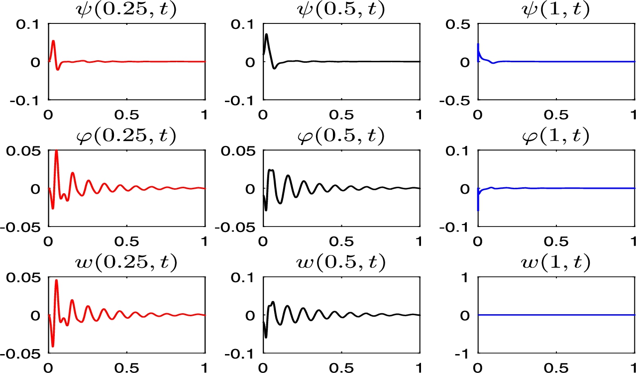
Test 1. and .
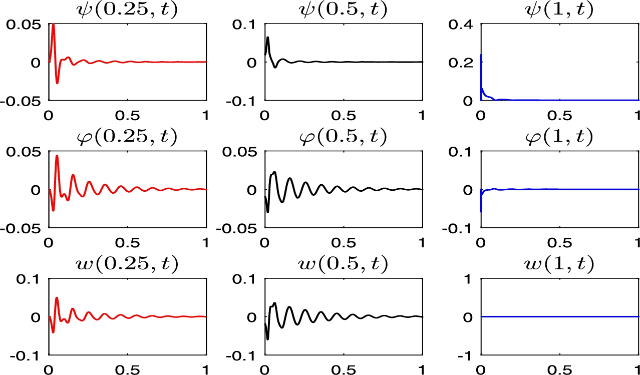
Test 2. and .
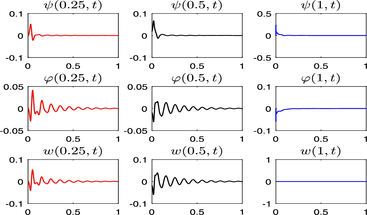
Test 3..
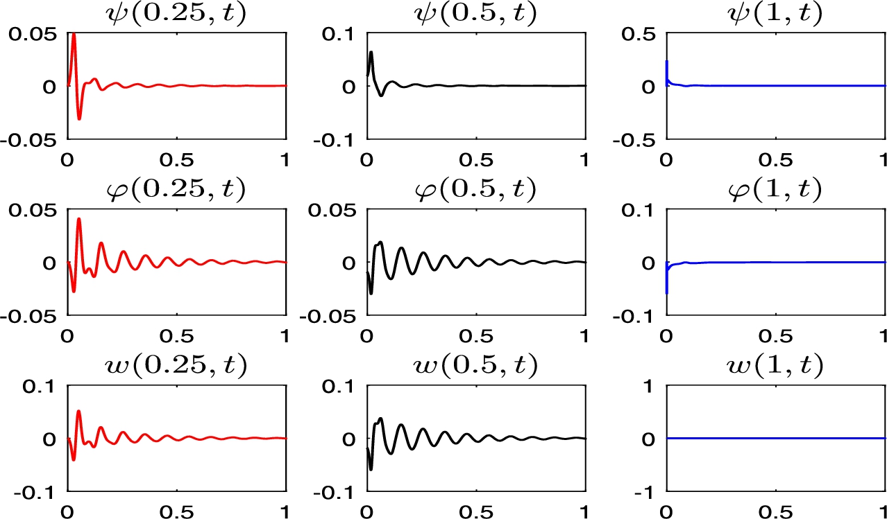
Test 4..
In order to ensure the scheme stability, we use a temporal and spatial steps satisfying the stability the Courant–Friedrichs–Lewy (CFL) inequality , where represents the time step and the spatial step. The spatial interval is subdivided into 200 subintervals, where the temporal interval is deduced from the stability condition above. We run our code for 10000 time steps using the following initial conditions:
TEST 1.
TEST 2.
TEST 3.
TEST 4.
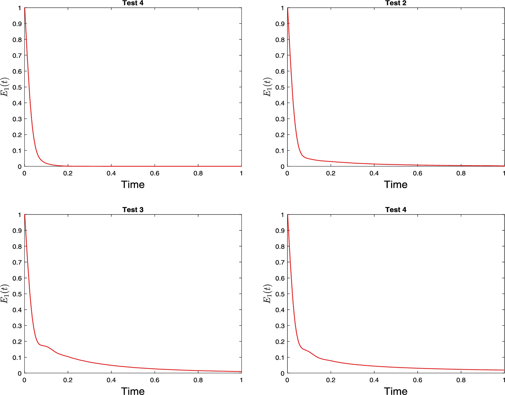
Energy functions for Tests 1, 2, 3 and 4.
In Fig. 1–4, we plot the damping behavior of the three waves φ, ψ and ω for the cross sections , and . Moreover, we have to mention that the cutting solution at , represent the non-Dirichlet memory boundary condition for φ and ψ. While represents the Dirichlet boundary condition for ω. In Fig. 5, we plot and compare the decay behavior of resulting energies for the Test 1–4.
As a final conclusion, we obtained an exponential decay for the Tests 1 and 2 and a polynomial decay for the Tests 3 and 4. This is consequence of the choice of the functions for and their values on the spacial interval .
Concluding remarks and open problems
In this paper, Bresse system with one damping and with memory-type boundary conditions was considered, we proved the well-posedness, stability results were proved under the condition of equal wave speeds, and some numerical approximations based on finite volume were presented to validate the theoretical results obtained in this paper. The proofs were based on multipliers techniques and the construction of Lyapunov functional. We need to mention here that the stability results for the same model under the memory-type boundary conditions only is an open problem, also the condition of equal wave speeds is it a necessary condition? It is an open problem as well.
Footnotes
Acknowledgement
The authors are grateful to the editor and referees for their comments which helped to improve the paper. This work was supported by MASEP Research Group in the Research Institute of Sciences and Engineering at University of Sharjah. Grant No. 2002144089, 2019-2020.
References
1.
M.Afilal, A.Guesmia and A.Soufyane, New stability results for a linear thermoelastic Bresse system with second sound, Appl. Math. Optim.83 (2021), 699–738. doi:10.1007/s00245-019-09560-7.
2.
M.Afilal, A.Guesmia, A.Soufyane and M.Zahri, On the exponential and polynomial stability for a linear Bresse system, Math. Methods Appl. Sci.43(5) (2020), 2626–2645. doi:10.1002/mma.6070.
3.
M.Afilal, T.Merabtene, K.Rhofir and A.Soufyane, Decay rates of the solution of the Cauchy thermoelastic Bresse system, Z. Angew. Math. Phys.67 (2016), Art. 119.
4.
F.Alabau-Boussouira and P.Cannarsa, A generalmethod for proving sharp energy decay rates formemory-dissipative evolution equations, C R Acad Sci Paris, Ser I.347 (2009), 867–872. doi:10.1016/j.crma.2009.05.011.
5.
M.O.Alves, L.H.Fatori, M.A.J.Silva and R.N.Monteiro, Stability and optimality of decay rate for a weakly dissipative Bresse system, Math. Methods Appl. Sci.38(5) (2015), 898–908. doi:10.1002/mma.3115.
6.
M.S.Alves, O.Vera, A.Rambaud and J.E.Muñoz Rivera, Exponential stability to the Bresse system with boundary dissipation conditions, arXiv:1506.01657.
7.
V.I.Arnold, Mathematical Methods of Classical Mechanics, Springer-Verlag, New York, 1989.
8.
A.Benaissa and A.Kasmi, Well-posedeness and energy decay of solutions to a Bresse system with a boundary dissipation of fractional derivative type, Discrete Conti. Dyna. Sys.-B23(10) (2018), 4361–4395.
9.
F.A.Boussouira, J.E.Muñoz Rivera and D.AlmeidaJr., Stability to weak dissipative Bresse system, J. Math. Anal. Appl.374 (2011), 481–498. doi:10.1016/j.jmaa.2010.07.046.
10.
J.A.C.Bresse, Cours de Mécanique Appliquée, Professé a L’école des Ponts et Chaussées, Par, M. Bresse, Gauthier-Villars, Paris, 2013, pp. 1865–1868.
11.
W.Charles, J.A.Soriano, F.A.F.Nascimento and J.H.Rodrigues, Decay rates for Bresse system with arbitrary nonlinear localized damping, J. Differential Equations255 (2013), 2267–2290. doi:10.1016/j.jde.2013.06.014.
12.
L.H.Fatori, M.O.Alves and H.D.Fernández Sare, Stability conditions to Bresse systems with indefinite memory dissipation, Appl. Anal.99 (2020), 1066–1084. doi:10.1080/00036811.2018.1520982.
13.
L.H.Fatori and R.N.Monteiro, The optimal decay rate for a weak dissipative Bresse system, Appl. Math. Lett.25(3) (2012), 600–604. doi:10.1016/j.aml.2011.09.067.
14.
L.H.Fatori and J.E.Muñoz Rivera, Rates of decay to weak thermoelastic Bresse system, IMA J. Appl. Math.75(6) (2010), 881–904. doi:10.1093/imamat/hxq038.
15.
B.Feng and M.Zahri, Optimal decay rate estimates of a nonlinear viscoelastic Kirchhoff plate, Complexity (2020), 6079507.
16.
F.A.Gallego and J.E.Muñoz Rivera, Decay rates for solutions to thermoelastic Bresse system of types I and III, Electr. J. Differential Equations2017 (2017), 73.
17.
K.F.Graff, Wave Motion in Elastic Solids, Dover Publications, New York, 1991.
18.
A.Guesmia, Asymptotic stability of Bresse system with one infinite memory in the longitudinal displacements, Mediterr. J. Math.14 (2017), 49. doi:10.1007/s00009-017-0877-y.
19.
A.Guesmia and M.Kafini, Bresse system with infinite memories, Math. Methods Appl. Sci.38 (2015), 2389–2402. doi:10.1002/mma.3228.
20.
A.Guesmia and M.Kirane, Uniform and weak stability of Bresse system with two infinite memories, Z. Angew. Math. Phys.67 (2016), Art. 124. doi:10.1007/s00033-016-0719-y.
21.
J.H.Hassan, S.A.Messaoudi and M.Zahri, Existence and new general decay results for a viscoelastic-type Timoshenko system, Zeitschrift für Analysis und ihre Anwendungen39(2) (2020), 185–222. doi:10.4171/ZAA/1657.
22.
K.P.Jin, Stability for locally coupled wave-type systems with indirect mixed-type dampings, Appl. Math. Optim.85 (2022). doi:10.1007/s00245-022-09830-x.
23.
K.P.Jin, J.Liang and T.J.Xiao, Coupled second order evolution equations with fading memory: Optimal energy decay rate, J. Diff. Equ.257 (2014), 1501–1528. doi:10.1016/j.jde.2014.05.018.
24.
K.P.Jin, J.Liang and T.J.Xiao, Uniform polynomial stability of second order integro-differential equations in Hilbert spaces with positive definite kernels, Discrete Conti. Dyna. Sys. Ser. S14(9) (2021), 3141–3166.
25.
K.P.Jin, J.Liang and T.J.Xiao, New general decay result for a class of neutral viscoelastic equations, J. Math. Anal. Appl.506(2) (2022), 125673. doi:10.1016/j.jmaa.2021.125673.
26.
A.Keddi, T.A.Apalara and S.A.Messaoudi, Exponential and polynomial decay in a thermoelastic-Bresse system with second sound, Appl. Math. Optim.77 (2018), 315–341. doi:10.1007/s00245-016-9376-y.
27.
J.E.Lagnese, G.Leugering and E.J.P.G.Schmidt, Modeling, Analysis and Control of Dynamic Elastic Multi-Link Structures. Systems & Control: Foundations & Applications, Birkhäuser Boston Inc., Boston, 1994.
28.
I.Lasiecka and D.Tataru, Uniform boundary stabilization of semilinear wave equation with nonlinear boundary damping, Differential Integral Equations8 (1993), 507–533.
29.
I.Lasiecka and X.J.Wang, Intrinsic decay rate estimates for semilinear abstract second order equations with memory, in: New Prospects in Direct, Inverse and Control Problems for Evolution Equations, Springer INdAM Series, Vol. 10, Springer, Cham, 2014, pp. 271–303.
30.
Z.Liu and B.Rao, Energy decay rate of the thermoelastic Bresse system, Z. Angew. Math. Phys.60 (2009), 54–69. doi:10.1007/s00033-008-6122-6.
31.
T.F.Ma and R.N.Monteiro, Singular limit and long-time dynamics of Bresse systems, SIAM J. Math. Anal.49(4) (2017), 2468–2495. doi:10.1137/15M1039894.
32.
S.A.Messaoudi and J.H.Hassan, New general decay results in a finite-memory Bresse system, Comm. Pure Appl. Anal.18(4) (2019), 1637–1662. doi:10.3934/cpaa.2019078.
33.
S.A.Messaoudi and A.Soufyane, Boundary stabilization of a nonlinear system of Timoshenko type, Nonlinear Anal.67 (2007), 2107–2121. doi:10.1016/j.na.2006.08.039.
34.
J.E.Muñoz Rivera and M.G.Naso, Boundary stabilization of Bresse systems, Z. Angew. Math. Phys.70 (2019), Art. 56.
35.
M.I.Mustafa, The control of Timoshenko beams by memorytype boundary conditions, Appl. Anal. (2019). doi:10.1080/00036811.2019.1602724.
36.
S.Rifo, O.V.Villagran and J.E.Muñoz Rivera, The lack of exponential stability of the hybrid Bresse system, J. Math. Anal. Appl.436 (2016), 1–15. doi:10.1016/j.jmaa.2015.11.041.
37.
M.L.Santos, Decay rates for solutions of semilinear wave equations with a memory condition at the boundary, Electron. J. Qual. Theory Differ. Equ.7 (2002), 17pp.
38.
M.L.Santos, Decay rates for solutions of a Timoshenko system with a memory condition at the boundary, Abstr Appl Anal.7 (2002), 531–546. doi:10.1155/S1085337502204133.
39.
J.A.Soriano, J.E.Muñoz Rivera and L.H.Fatori, Bresse system with indefinite damping, J. Math. Anal. Appl.387 (2011), 284–290. doi:10.1016/j.jmaa.2011.08.072.
40.
C.C.S.Tavares and M.L.Santos, On the Kirchhoff plates equations with thermal effects and memory boundary conditions, Appl. Math. Comput.213 (2009), 25–38.
41.
T.J.Xiao and J.Liang, Coupled second order semilinear evolution equations indirectly damped via memory effects, J. Differential Equations254(5) (2013), 2128–2157. doi:10.1016/j.jde.2012.11.019.