We consider massless Dirac operators on the real line with compactly supported potentials. We solve two inverse problems: in terms of zeros of reflection coefficient and in terms of poles of reflection coefficients (i.e. resonances). Moreover, we prove the following:
1) a zero of the reflection coefficient can be arbitrarily shifted, such that we obtain the sequence of zeros of the reflection coefficient for another compactly supported potential,
2) the set of “isoresonance potentials” is described,
3) the forbidden domain for resonances is estimated,
4) asymptotics of the resonances counting function is determined,
5) these results are applied to canonical systems.
We consider inverse problems for Dirac operators on the real line with compactly supported potentials. Such operators have many physical and mathematical applications. These Dirac operators are also known as Zakharov–Shabat (or AKNS) systems, which were used by Zakharov and Shabat [48] to study the nonlinear Schrödinger (NLS) equation (2.9) (see also [1,8,11]). In our paper, we consider the self-adjoint Dirac operator H on given by
The potential Q has the following form
where the class is defined for some fixed throughout this paper by
is a set of all functions such that the convex hull of equals for some . The set is equipped with the metric given by
Note that is a metric space, which is not complete. Recall known results about Dirac operators H, see e.g., [35]. The spectrum of H satisfies . We introduce the matrix-valued Jost solutions of the Dirac equation
under the standard condition for compactly supported potentials:
The equation (1.4) has exactly one linear independent matrix-valued solution, then there exists a unique transition matrix such that
The transition matrix A has the form
where we have used the notation , . It is known that a and b are entire, for any and a has zeros in , which are called resonances. Note that the resonances are also zeros of Fredholm determinants and poles of the resolvent (see e.g. [19]). Due to (1.5) the zeros of b and a do not coincide. Let be the free Dirac operator on . The scattering matrix S for the pair H, is given by
Here is a transmission coefficient and (or ) is a right (or left) reflection coefficient. The matrix-valued function S admits a meromorphic continuation from onto , since a and b are entire. Poles of S are resonances and zeros of the reflection coefficients coincide with zeros of b or .
Main goal
Our main goal is to solve the inverse problem for Dirac operators with compactly supported potentials in terms of resonances. We sometimes write , , … instead of , , when several potentials are being dealt with. We show that the resonances of operator H do not uniquely determine the potential, and then we need additional data. We consider inverse problems for the following mappings:
the mapping ,
the mapping ,
the mapping for any sign ±.
We need to underline that in order to solve the inverse problem ii) in terms of resonances, we need to solve the problem i). An inverse problem is to determine the potential by some data, and it consists of at least the four parts:
Uniqueness. Do data uniquely determine the potential?
Reconstruction. Give an algorithm to recover the potential by data.
Characterization. Give necessary and sufficient conditions that data correspond to a potential.
Continuity and stability. Show that a potential is a continuous function of data and describe how data can be changed so that they remain data for some potential.
The data considered in our paper can be divided into two sets, and we will briefly describe the results obtained for each of them.
Firstly, we consider the inverse problem in terms of a function b (or the zeros of b, and also the reflection coefficients ). For these data, we obtain the following results:
The function b (or the zeros of b, or one of the reflection coefficients ) determines a potential from uniquely.
We solve the reconstruction and characterization problem.
We also solve these problems for even, odd or real-valued potentials.
We solve the continuity problem in terms of b, and we partially solve this problem in terms of zeros of b. Namely, we show that if a zero of b is arbitrarily shifted, then we obtain a coefficient for some potential from . We also prove that a potential continuously depends on one zero of b, while other zeros are fixed.
Secondly, we consider the inverse problem in terms of the function a (or in terms of the resonances). We obtain the following results:
Since a does not uniquely determine a potential from , we need to introduce additional data: a sequence , where for some and , , where . In a generic case, is a phase multiplier of b and and are multiplicities of zeros and of b, where is a sequence of zeros of b in .
We solve the characterization problem for such extended data and describe isoresonance sets, i.e. the sets of potentials which have the same resonances.
We also solve these problems for even, odd or real-valued potentials.
Finally, we consider the stability problem for resonances. Note that the resonances do not completely determine a potential, and they are not free parameters of the Dirac operator, i.e. we cannot arbitrarily move a resonance. On the other hand, the zeros of b completely determine a potential, and they are free parameters.
The coefficients a and b are important to study the NLS equation. Namely, and , , are action and angle variables for the NLS equation (see e.g. p. 230 in [11]). For we obtain the representations of action-angle variables in terms of resonances and zeros of b.
We solve the inverse problem for the Dirac operators with potentials, which have some symmetries in Section 6. We show that the resonances uniquely determine a real-valued even or real-valued odd potential up to a sign.
Note also that Dirac operators can be rewritten as canonical systems (see, e.g., p. 389 in [15]). Due to this relation, we describe the class of canonical systems, which are unitary equivalent to the Dirac operators in Section 7. Then we introduce the scattering matrix and solve the inverse resonance problem for such canonical systems.
Historical review
There are a lot of results about a one-dimensional case, see [10,13,16,25,42,49] and references therein. The inverse resonance problem, including reconstruction and characterization, for Schrödinger operators with compactly supported potentials was solved for the case of the half-line in [25] and for the case of the real line in [27]. The stability problems for resonances of Schrödinger operators were considered in papers [25–27,37]. The inverse resonance scattering was discussed for Schrödinger operators with model potentials perturbed by compactly supported potentials. The following model potentials were considered: step potentials [6], periodic potentials [28], linear potentials (corresponding to one-dimensional Stark operators) [31]. The inverse resonance problem for the Laplacian on rotationally symmetric manifolds was considered in [22]. Resonances for three and four-order differential operators with compactly supported coefficients were discussed in [2,3,32]. Results about the Carleson measures for resonances were obtained in [30]. We also mention other results about resonances: [5,9,46,47].
Now, we briefly review results on resonances for one-dimensional Dirac operators. Global estimates of resonances in terms of the norm of the potential and the diameter of its support for the massless Dirac operators on the real line with compactly supported potentials, via the Carleson measures arguments, were obtained in [29]. Resonances for this operator were studied in [19] under stronger condition and for the massive Dirac operators on the half-line in [20]. Note that this condition is crucial since in this case the second term in the asymptotic expansion of the Jost solutions of the Dirac operators decrease as in the case of Schrödinger operator for the large spectral parameter, and it provides suitable estimates of the Jost functions. In these papers and in paper [21], devoted to radial massive Dirac operators, the following results were obtained:
asymptotics of counting function of the resonances;
estimates on the resonances and the forbidden domain;
the trace formula in terms of resonances for the massless case.
Finally, the inverse resonance problem for the massless Dirac operator on the half-line with compactly supported potentials was solved in [33]. In this paper asymptotics of counting function of the resonances and the forbidden domain for resonances were obtained without smoothness condition on the potential. The stability of this inverse resonance problem was considered in paper [38]. Note that the one-dimensional Dirac operator can be used to study the resonances in other related problems, see, e.g., [18].
We discuss now canonical systems. Recall that Dirac operators can be transformed to canonical systems, for which the inverse problem can be solved in terms of de Branges spaces (see [7,41]). There exist many papers devoted to the inverse problem for canonical systems, see [4,33,36,40] and references therein. In particular, in [40] it was used to study the inverse spectral problem of Schrödinger and Dirac operators.
Moreover, relations between Jost functions and de Branges spaces and the characterization of de Brange spaces associated with the Schrödinger operators were given in paper [4] (see also [36]) and for the case of Dirac operators in [33].
Main results
Inverse problems
We define the Fourier transform and its inverse on by
We introduce classes of scattering data associated with zeros of reflection coefficients.
is the metric space of all entire functions u such that equipped with the metric given by
Note that the metric space is not complete. We recall needed facts about entire functions. An entire function is said to be of exponential type if there exist constants such that , . We introduce the Cartwright class of entire functions by
is a class of entire functions f of exponential type such that
where .
We shortly describe needed properties of functions from the Cartwright class. Let and let ν be the multiplicity of zero of at . Let be zeros of f in counted with multiplicity and labeled by
Then f has the Hadamard factorization (see, e.g., pp. 127–130 in [34])
where the product converges uniformly on compact subsets of and
We denote the number of zeros of function f having modulus less than r by , each zero being counted according to its multiplicity. For any function , the Levinson theorem holds true (see, e.g., p. 58 in [23]):
We present our first result.
The mappingis a homeomorphism betweenand.
1) The proof of this theorem consists of two parts. Firstly, we solve the inverse scattering problem for the Dirac operators with potentials from , see Theorem 2.3. Secondly, we prove that there exists a one-to-one correspondence between b and , and to get this result we use arguments from [27].
2) In Corollary 6.2, we give the characterization of b for even, odd or real-valued potentials.
3) We discuss the recovery procedure for this inverse problem in Section 3.
Now we introduce the class of scattering data associated with the resonances, i.e. the poles of the reflection coefficients.
is the set of all entire functions f such that:
for any ;
for any ;
;
.
We consider the inverse problem for the Dirac operator H in terms of . The idea here is to construct for given such that and then we can determine a potential using Theorem 2.1. So let be given and let . Thus, to determine a potential we need to solve the equation . However, in general, this equation has many solutions . It follows that the coefficient a does not uniquely determine a potential and to obtain a unique solution of the equation we need additional information about b.
We consider the function B. It is easy to see that B is an exponential type function, for each and the zeros of B are symmetric with respect to the real line. Let be a solution of the equation . Then some zeros of B are zeros of b, and the other are zeros of . We will show that this information is sufficient to obtain a unique solution of this equation. Namely, if the multiplicities of the zeros of b in are fixed then there exists a unique solution of the equation . Note also that zeros on the real line are the same for all solutions.
We construct the data for any . Let be the zeros of in counted without multiplicity and labeled by
and let be theirs multiplicities. Recall that . Let also be the multiplicity of the zero of . Then we introduce a mapping by
where is the multiplicity of the zero of b and is the multiplicity of the zero of b. Note that for each and shows how the zero of B is allocated between b and and is a general phase multiplier.
Now for any given we construct the set , where , such that for any there exist a solution b of the equation and . We introduce as follows
where
Here is a unite circle in and is, in some sense, its discrete analogues. Now, we give our second main result.
The mappinggiven by (
2.6
) is a bijection betweenand, where,, and.
1) In order to construct the set , we need to know the function a. Thus, to obtain a unique potential we need to choose , construct , , by (2.7) and then we need to choose .
2) Corollary 6.4 gives the characterization of a for even, odd or real-valued potentials and we will show how is reduced in these cases.
3) The inverse resonance problem was solved for the Schrödinger operators on the half-line [25] and on the line [27]. The inverse resonance problem for the Dirac operator on the half-line was considered in [33]. In the proof we use arguments from [25,33] and mainly from [27]. Note that the case of half-line is simpler than the case of the real line since we have:
∙ the scattering matrix depends on two coefficients a and b;
∙ the potential is not uniquely determined by resonances.
These features lead to significant modification of methods given in [33]. Moreover, arguments from [27] required big changes since there are differences between Dirac and Schrödinger operators. Mainly it is the second term in the asymptotic expansion of the Jost solutions of the Dirac equations, which decreases more slowly for the large spectral parameter. Roughly speaking, it means that the spectral problem for Dirac operators corresponds to the spectral problem for the Schrödinger operators with distributions.
Using Theorems 2.1 and 2.2, we give the characterization of the reflection coefficients for the compactly supported potentials. We introduce the following classes.
(or ) is a set of all meromorphic functions (or ), given by (or ) for some such that
Below, we prove that for any . Thus, we introduce the metric
Note that equipped with the metric are incomplete metric spaces.
The mappingsare homeomorphisms betweenand.
The Paley–Wiener Theorem (see e.g. p. 30 in [23]) gives that and . Thus, using the properties of , we get the following corollary.
i) The potentialis uniquely determined by zeros ofand, where ν is the multiplicity of zero ofat.
ii) A potentialis uniquely determined by, whereare zeros ofandfor.
iii) Let. Then the functionssatisfy (
2.3
–
2.4
).
The asymptotics of distribution of resonances of the Dirac operators on the real line was obtained in [19] for compactly supported potentials . Recall that for Schrödinger operators on the real line such results were obtained in [49].
It follows from Theorem 2.2 that for some there exist distinct potentials such that . Moreover, by Corollary 2.4, the function is uniquely determined by its zeros. For any , we introduce an iso-resonance set in by
Using Theorem 2.2 for fixed , we give the characterization of in terms of .
Let. Then the mappinggiven by (
2.6
) is a bijection betweenand, where,, and.
On the other hand, it follows from Theorem 2.1 that for each there exists a unique . Now, we describe how changes for .
Letand letbe zeros ofincounted without multiplicity and labeled by (
2.5
). Let also, where,. Thenif and only if, wherefor someandsuch that,,.
It is easy to see that P is a meromorphic function such that , which yields that for each and then for each we obtain
The NLS equation
Using analytical properties of a and b, we obtain representations of action-angle variables for the nonlinear Schrödinger equation (NLS equation) in terms of resonances and zeros of b. We recall some known facts about the NLS equation from [11]. Let be a solution of the defocusing NLS equation
satisfying the initial condition . For such equation, there exists the Lax pair and the Dirac operator is the corresponding self-adjoint operator. Thus, considering the solution of (2.9) as a potential of the Dirac operator H, we get , and these functions have a simple dynamics:
see, e.g., p. 52 in [11]. Note that there are differences in notations. Namely, if we denote by and the coefficients of the transition matrix, which was used in [11], then we get
Thus, solving the inverse problem for b given by (2.10), we obtain . Moreover, the NLS equation is a Hamiltonian system with the following Hamiltonian
Such system is completely integrable and there exist action variables and angle variables , , given by
where (see, e.g., p. 230 in [11]). Note that there is the ambiguity in the definition of at zeros of on the real line but it can be avoided by introducing new variables (see formula (7.9), p. 230 in [11]). Now, we give the representation of these variables in terms of resonances and zeros of b, when .
Letfor someand letbe its zeros incounted with multiplicities and labeled by (
2.2
). Then the action variablehas the formwhere the series converges uniformly on compact subsets of.
Let in addition,,, whereis defined by (
2.6
). Letbe zeros ofincounted without multiplicities and labeled by (
2.5
) and letbe zeros of B incounted with multiplicities. Then the angle variable has the formwhereand the series converges uniformly on compact subsets of.
1) It follows from (2.10) that if , then and are entire functions for any . Moreover, their zeros do not move when t changes.
2) If , then is not exponential type as function of k for any . Thus, by Theorem 2.1, is not compactly supported for any .
Location of resonances
Now, we describe locations of resonances and zeros of b. Firstly, we discuss a forbidden domain for resonances.
Letbe resonances for someand let. Then each, satisfiesfor some constant, which does not depend on n. In particular, for any, there are only finitely many resonances in the strip
If , then the forbidden domain associated with (2.14) can be clarified (see Theorem 1.3 in [19]).
Secondly, we describe some automorphisms of the classes and . We show that the zeros of b are free parameters and prove that b continuously depends on a zero.
Letand letbe zeros ofcounted with multiplicities and labeled by (
2.2
). Let,, for some. Then there exist a uniqueand a uniquesuch thatIn particular, any point oncan be a zero of b with any multiplicity for some. Moreover, if each,, then we have
For Schrödinger operator, similar results are obtained in [27].
Now, we consider resonances. In general, the resonances of Dirac operators on the real line are not free parameters. If potential is odd, even or real-valued, then for any (see Lemma 6.1). In this case, the resonances are symmetric with respect to the imaginary line. We introduce the following class
For potentials q such that , we prove that a resonance can be shifted in some direction.
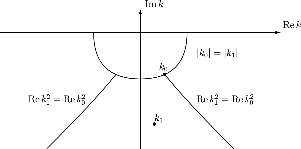
Letfor someand letfor some. Assume thatsatisfiesThen there existssuch thatand
Let and . Then inequalities (2.15) have the following form (see also Fig. 1):
Note that in any neighborhood of there exist such (2.16) holds true and such that (2.16) does not hold true.
In this section, we recall results about the inverse scattering problem for the Dirac operator on the real line. We introduce the following Banach spaces equipped with the corresponding norms:
We also define the following Banach algebras with pointwise multiplication equipped with the corresponding norms:
It is well-known that and are unital Banach algebras (see e.g. Chapter 17 in [14]). We denote by the space of matrices with complex entries.
Jost solutions
We consider Dirac operator on , where the potential Q has form (1.2) and . For and , we also introduce the Jost solutions of Dirac equation
satisfying asymptotic conditions:
For each and there exist Jost solutions, and they have integral representations in terms of the transformation operators. We recall these known results, see p. 39 in [11] and Proposition 3.5 in [12].
Let. Then Jost solutionshas the formfor somesuch thatMoreover, for each, the following statements hold true:
For each fixed, the mappingsfromintoare continuous and, for any, they satisfy:where
For each fixed, the mappingsfromintoare continuous;
For each fixed, the mappingsfromintoare continuous and satisfy:
This lemma gives that there exist matrix-valued Jost solutions only for . However, we can construct the vector-value Jost solutions for any or . It follows from the Paley–Wiener Theorem and representation (3.3). Thus, we give the following lemma (see e.g. Proposition 3.7 in [12]).
Let. Then, for any fixed, the functionsandadmit analytical continuation fromontoand the functionsandadmit analytical continuation fromonto.
Transition matrix
Since equation (3.1) has exactly one linear independent matrix-valued solution, it follows that for any there exists a unique transition matrix such that
Using Lemma 3.1, we obtain known representation of the matrix . In order to formulate this result, we introduce the following classes.
is a metric space equipped with the metric
is a metric space equipped with the metric , where is the set of all analytic on and continuous on functions a such that:
for any ;
for any ;
;
;
and the metric is given by
Note that and isometrically.
Thus, we formulate the following known lemma (see, e.g., [12]).
Letand let A be given by (
3.7
). Then A has the following form:and the mappingsfromintoandfromintoare continuous.
Moreover, letfor some. Then the following representations hold true:
Recall that the determinant of any matrix-valued solution of (3.1) is constant, and then for any . Thus, we have
Substituting (3.3) in (3.10) and using (3.4), we get that the matrix have the following form:
where and and representation (3.9) holds true. By Lemma 3.1, i), we have for each and then , . Thus, we get .
Now, we check the other conditions of . Since , it follows that , which yields . This implies that for any and . Using (3.7), we obtain the following representation:
Due to Lemma 3.2 and (3.11), the function a admit an analytical continuation from onto . We show that for any . It follows from (3.11) that if for some , then the vector-valued solutions and are linearly dependent. Moreover, due to (3.2), they exponentially decrease as for any . Thus, if for some , then k is an eigenvalue of H. Since H is self-adjoint, it has no eigenvalues in . Thus, for any and then .
Finally, it follows from Lemma 3.1, ii), that the mappings from into are continuous for each and each fixed . Due to (3.9), we get that the mappings from into and from into are continuous. □
Note that is invertible if and only if for any (see e.g. Lemma 2.9 in [17]). Moreover, the inverse mapping is continuous on the subspace of invertible elements of Banach algebra (see, e.g., Chapter 2 in [14]). Since , we get the following.
Letand let. Then the mappingfromintois continuous. In particular, there exists a uniquesuch that
Now, we show that a and b are not independent. In order to get this result, we need the following known lemma about the Banach algebra (see e.g. Chapter 6 in [14]).
Letand let Ω be an open neighborhood of the closure of the range of f. Let ϕ be an analytic function on Ω. Then we have. Moreover, the mappingis a continuous mapping on the subspace of all functionsuch that its ranges are contained in Ω.
In particular, we obtain the following corollary for the logarithm and the exponential function. We introduce subspaces of :
We also introduce the mappings , , and , , where we fixed the branch of the logarithm by for any .
The mappingsandare continuous.
It is well-known that the Fourier transform of any integrable function is uniformly continuous. Thus the range of any is a compact subset of and then, by Lemma 3.5, log is a continuous mapping from to . Moreover, it follows from the Riemann–Lebesgue lemma (see e.g. Theorem IX.7 in [39]) that as for any and then as . Thus, we have .
For any , the range of f is a compact subset of and then, by Lemma 3.5, exp is a continuous mapping from to . As above, as for any and then as . Since for any , it follows that . □
We also introduce the Cauchy integral operator on by
where the limit is taken in . It is well-known that has the representation:
where is the indicator function of . We need the following known lemma.
The mappingfromintois continuous.
Let . Using (3.13), we get . Since the mapping from to is continuous, we get the statement of the lemma. □
We also need the following technical lemma.
Letand letfor any. Then there exists a unique solutionof the equation. Moreover, the mappingfromintois continuous.
Firstly, we prove the existence and continuity. It is easy to see that . Thus, it follows from Corollary 3.6 that and the mapping from into is continuous. We introduce
It follows from Corollary on p. 128 in [24] that F is analytic on and as and , for almost all . Moreover, it follows from Lemma 3.7 that , where , and F depends continuously on .
Now, let . Then it follows from Corollary 3.6 that and a depends continuously on . It also follows that a is analytic in and for any . Since for any and , we have that for any and . Thus, we have . Recall that F depends continuously on h and then a also depends continuously on h.
Secondly, we prove the uniqueness. Let be a solution of the equation . Then is an analytic function in and then is a harmonic function in and it is a uniquely determined by its boundary value . Since is a connected open subset, it follows that has a unique harmonic conjugate up to the constant. Thus, if is another solution of the equation , which is analytic in and as , then we have for some . Due to and as , it follows that and as for some . Then for any for some and then . □
Now, we show that for any there exists a unique such that the determinant of the associated transition matrix equals 1.
Let. Then there exists a unique solutionof the equationMoreover, the mappingfrominis continuous.
Let . Then it follows from the basic properties of Banach algebras that and h depends continuously on . Due to , we have . At last, we have for any . Thus, it follows from Lemma 3.8 that there exists a unique solution of the equation (3.14) and it depends continuously on b. □
Note that a similar result for compactly supported potentials can be obtained using the theory of entire functions (see, e.g., Theorem 2.3 in [27]).
Direct scattering
Recall that on is the free Dirac operator. The scattering matrix for the pair , H has the following form
Here is the transmission coefficient and (or ) is the right (or left) reflection coefficient. We introduce the following class of all reflection coefficients.
is a metric space of all functions such that for any equipped with the metric
It follows from the definition of the scattering matrix that it can be obtained from the transition matrix. Due to Corollary 3.4, the transmission coefficient and it depends continuously on . Now, we show that the reflection coefficient also depends continuously on and . Note that this result is also well-known (see e.g. [12]).
Let,be such that. Then we haveanddepends continuously onand.
Since and , we have . By Lemma 3.4, . Due to , we get and then . It follows from Corollary 3.4 that is a continuous mapping from to . Moreover, the multiplication and the complex conjugate are also continuous mappings from to . Then depends continuously on a and b. □
On the other hand, the coefficients a and b are uniquely determined by the reflection coefficient.
Let. Then there exist a unique solutionof the equationand the mappingfromintois continuous. Moreover, in this caseand b depends continuously on.
It follows from (3.15) that
Due to , for any , we get for any . Using the multiplication properties of the Banach algebra, we have . Note that is invertible if and only if for any (see e.g. Lemma 2.9 in [17]). Since and for any , it follows that and then and it depends continuously on . It follows from the Riemann–Lebesgue lemma that as . Since for some , we have that . Recall that for any . Hence, we obtain . Due to , we have and then . Thus, by Lemma 3.8, there exists a unique solution of the equation (3.15) and it depends continuously on . Finally, using the multiplication properties of the Banach algebra, we get and b depends continuously on . □
Above, we considered only the right reflection coefficient. However, the left reflection coefficient is uniquely determined by the right one. We introduce the mapping from in , where a is given by Lemma 3.11. The following result holds true (see e.g. Lemma 3.4 in [12]).
The mappingis a homeomorphism and, whereis the identity mapping on.
It follows from Lemmas 3.11, 3.12 that we can recover the scattering matrix from one reflection coefficient. Moreover, by Lemmas 3.9, 3.10, we can recover the reflection coefficient from the coefficient and then the scattering matrix too.
Inverse scattering
Now, we give the solution of the inverse scattering problem for the Dirac operators (see e.g. Theorem 1.1 in [12]).
The mappingsare homeomorphisms betweenand.
It follows from this theorem that a potential is uniquely determined by the right or left reflection coefficient. Thus, it solves the uniqueness, the characterization and the continuity problems for potentials from in terms of the reflection coefficients. Using this result, we solve the inverse problem in terms of the coefficient b.
The mappingis a homeomorphism betweenand.
We consider the composition of mappings:
Using Theorem 3.13 and Lemma 3.11, we get that for any there exists a unique and depends continuously on q. On the other side, we consider the composition of mappings:
Using Lemmas 3.9, 3.10, and Theorem 3.13, we get that for any there exists a unique such that and q depends continuously on b. □
In order to recover a potential from the reflection coefficient, one can use the Gelfand–Levitan-Marchenko (GLM) equation. For any , we introduce the matrix-valued functions
where . The following result was also obtained in [17].
Letandfor someand for any. Thenandsatisfy the GLM equations:for eachand almost all.
Letbe given by (
3.16
) for some. Then equation (
3.17
) has a unique solutionand this solution depends continuously on. Moreover, the mappingfromintois continuous.
Letbe given by (
3.16
) for some. Then equation (
3.18
) has a unique solutionand this solution depends continuously on. Moreover, the mappingfromintois continuous.
Letsuch that. Then we get
One can recover a potential q from the reflection coefficient as follows:
In this section, we show the relationship between the support of a potential and properties of the transition and scattering matrix. Firstly, we show that a potential is compactly supported if and only if the associated kernels are compactly supported.
Letand let. Then we have for any:
if and only iffor almost allsuch that;
if and only iffor almost allsuch that.
i) Let . Then it follows from (3.5) that for each , . Thus, for each and for almost all . Substituting this identity in (3.17), we get for each and for almost all , i.e. for almost all . Now substituting this identity in (3.17), we get for almost all such that .
Let for almost all such that . By Lemma 3.15 the mapping is continuous. Combining these facts, we get for almost all , which yields, by Lemma 3.1, that for almost all .
ii) In this case, the proof is similar. □
The support of a potential is also related to the support of and .
Letand let,. Then we have
Firstly, we show that . If , then the inequality is evident. Let for some . Due to (3.16), we have for any . Substituting this identity in (3.17), we get for almost all such that . Thus, by Lemma 4.1, .
Secondly, we show that . Let . It follows from (3.12) and that
where , and . Using , , and well-known property , we get . Substituting these inequalities in (4.2), we have .
Thirdly, we show that . Let . Then, by Lemma 4.1, for almost all . Using (3.9), we get .
Combining these three inequalities, we obtain the first line in (4.1). The proof of the second line in (4.1) is similar. □
In Lemma 3.9, we proved that for any there exists a unique such that . Now, we show that if , then the corresponding a belongs to . Recall that and was defined in Section 2. Recall also that we introduced the Cartwright classes of entire functions with fixed types in Section 2. Now, we define the more general classes.
For any , is a class of entire functions of exponential type f such that
where .
Note that .
If for some , then it also has the Hadamard factorization. Let be the multiplicity of zero of f. We denote by zeros of f in counted with multiplicity and labeled by (2.2). Then f has the Hadamard factorization
see, e.g., pp. 127–130 in [34], where the product converges uniformly on compact subsets of and
Let. Then there exist a unique solutionof the equationMoreover, the mappingfromintois continuous.
Due to Lemma 3.9, there exists a unique solution of equation (4.3) for and it depends continuously on . Thus, we only need to show that and it is a solution of (4.3) for any .
Let , . Since , it follows that , and then and the following properties hold true:
( iff , );
for any .
Here we used the following simple facts about conjugate functions:
Let , be the zeros of A in counted with multiplicity and labeled by (2.2). Then the Hadamard factorization for A has the following form
where the product converges uniformly on compact subsets of , the constant , and
We introduce
Due to (4.5), we have
and then, by the Lindelöf theorem (see, e.g., p. 21 in [23]), the product in (4.6) converges uniformly on compact subsets of and , where . Using (4.4) and (4.6), we get , i.e. is a solution of (4.3) for any . It follows from (4.3) that and then, using , we get , .
Note that in the proof of Lemma 3.8, we show that if and are analytic in , , , , and they are solutions of (4.3), then for some . Thus, it follows that for some , which yields . Since , there exist such that . Due to , it follows from the Paley–Wiener Theorem that and then . □
Above, we recover the coefficient a from b. Now, we show that the coefficient b is uniquely determined by a with additional data. Recall that the space was introduced in Section 2.
Letand let. Then there exists a unique solution,, of the equation
Let , . Since , it follows that , and then and the following properties hold true:
( iff , );
for any .
Let be the zeros of B in counted without multiplicity and labeled by (2.5) and let be their multiplicities. Let be the zeros of B in counted without multiplicity and labeled by (2.5) and let be theirs multiplicities. Due to (ii), the real zeros of B have even multiplicity and then for each . Let also be the multiplicity of the zero of B. Then it follows from (ii) that . Due to , it has the following form
Then the Hadamard factorization for B can be written as follows:
where the product converges uniformly on compact subsets of , the constants and
It follows from the last inequality that
We introduce
Now, we consider
Thus, due to (4.9) and (4.10), we have
and then, by the Lindelöf theorem (see e.g. p. 21 [23]), the product in (4.11) converges uniformly on compact subsets of and , where . Using (4.8) and (4.11), we get , i.e. b is a solution of (4.7). It follows from (4.7) that and then , . Let be another solution of equation (4.3) such that and . Since the function from is uniquely determined by its zeros and by , it follows that .
Now, we show that . Due to , we get and then . Since and , it follows from the Paley–Wiener theorem that for some , which yields . □
Proof of the main theorems
In Theorem 3.14, we have shown that the mapping is a homeomorphism between and . Since the metrics on and and on and are equivalent, we only need to prove that the restriction of this mapping on is a bijection between and . Due to Theorem 3.14, if , then we have . Using Lemma 4.2, we get
which yields that and then we have .
Let . Then, by Theorem 3.14, there exists a unique such that . Since , we have . Then it follows from Lemma 4.2 that
which yields that . □
Let . By Theorem 2.1, we have and then there exists a unique , where . Since and is a solution of , it follows from Lemma 4.3 that .
Let , where . Due to Lemma 4.4, there exists a unique solution of the equation such that and then, by Theorem 2.1, there exist a unique such that . Moreover, it follows from Lemma 4.3 that is uniquely determined by as a solution of the equation . Hence, we have . □
Due to Theorem 3.13, the mappings are homeomorphisms between and . Since the metrics on and and on and are equivalent, we only need to prove that the restrictions of these mappings on are bijections between and .
Let . Using Theorems 2.1 and 2.2, we have and . Since and and a meromorphic function admits a unique continuation from to , it follows from the definitions of that .
Let . Then, by the definitions of , there exist and such that and (or ). Using Theorems 2.1 and 2.2, we get that there exists a unique such that and . Moreover, due to Lemmas 3.11 and 3.12, a and b are uniquely determined by (or ). Hence, we get . □
i) By Theorem 2.1, each is uniquely determined by . Hence, we get and it follows from the Paley–Wiener Theorem that and it satisfies (2.3 – 2.4). Due to (2.3), is uniquely determined by its zeros, by the multiplicity p of the zero of b, and by .
ii) By Theorem 2.2, each is uniquely determined by and by , where . Hence, we get for some and it follows from the Paley–Wiener Theorem that and it satisfies (2.3 – 2.4). Recall that if , then , , , and as . Thus, using (2.3), we see that is uniquely determined by its zeros. □
By Theorem 2.2, the mapping is a bijection between and , where , , and . Let . We consider the restriction of the mapping onto . It follows from the definition of that for any and then the mapping is a bijection between and , where . □
Let for some . Then we have and are solutions of the equation . Let be the zeros of in counted without multiplicity and labeled by (2.5) and let be their multiplicities. Let be the zeros of B in counted without multiplicity and labeled by (2.5) and let be theirs multiplicities. Let also be the multiplicity of the zero of B. Let and , where , for each . Due to (4.11), we have
which yields
where . We introduce , . Using , we get , . Since , we have for each , which yields that P has form (2.8).
Now, let , , and let and be zeros of and , be theirs multiplicities given as above. Let also , where for each . Let be given by (2.8). We introduce as follows
Since and for each , we have , , and then . Thus, by Theorem 2.2, there exists a unique such that and and then . Moreover, in this case, we have
Thus, as above, we see that . □
Let . Then and it has the Hadamard factorization (4.6):
for some , where the product converges uniformly on compact subsets of . Since absolute value is a uniformly continuous function, we have
where the product converges uniformly on compact subsets of . Recall that . Using well-known properties of the logarithm of infinite product (see, e.g., p. 16 in [44]), we get
for some , where we fixed the branch of the logarithm by for and its imaginary part belongs to and the series converges uniformly on compact subsets of . Substituting in (5.1), we get and then we obtain (2.11).
Let be the zeros of in counted without multiplicity and labeled by (2.5) and let be their multiplicities. Let be the zeros of B in counted without multiplicity and labeled by (2.5) and let be theirs multiplicities. Let also be the multiplicity of the zero of B. Let , where for each . Recall that and it has the Hadamard factorization (4.11):
for some , where the product converges uniformly on compact subsets of . Let be an open interval such that for any . Then we have
which yields
Using (5.2) and well-known property of logarithmic derivative of infinite product, we get
which yields
where the series converges absolutely and uniformly on compact subsets of , since (4.9) holds true.
Using (5.3) and (5.4), we can calculate between its zeros on . Since b is entire, it has finitely many zeros on any compact interval.
Now, we describe how changes in neighborhood of its zero. Let be a zero of b with the multiplicity . Then we have as . Using this asymptotics, we obtain
Combining (5.3) and (5.5), we get
where I and w are given by (2.13). Finally, if , then it follows from (5.2) that , which yields (2.12). □
Let . By Theorem 2.2, and then there exists such that . It is well-known that the set of smooth compactly supported functions is dense in . Thus, for any , there exists such that and . Let for some . Then we have . Estimating the left-hand side of this identity, we get
Since , we obtain
Using , we have
Substituting (5.7) and (5.8) in (5.6), we get
which yields (2.14). Now we consider (2.14) for . For fixed and , we get
Thus, there are finitely many resonances such that . Since it holds for any , we complete the proof of the theorem. □
For simplicity, we consider the case when . We introduce
Firstly, we show that , where for some . Since b is entire and , it follows that is entire. Using the definition of , we have
where , since as . Thus, we get . Now, we show that . Since , it follows that, for any , there exists such that for each . Note that for each . Using these estimates, we get
which yields . It follows from the Paley–Wiener Theorem that for some and then we get . Thus, by Theorem 2.1, there exists a unique such that .
Secondly, we show that . As above, we get . Now, we show that . Using , we obtain
Using (5.9) and , we get and then we have . Thus, it follows from Theorem 2.1 that there exists a unique such that .
Thirdly, we show that as . Using (2.1), (5.9), and the Plancherel theorem (see e.g. Theorem IX.6 in [39]), we get
Thus, it follows that as . By Theorems 2.1 and 3.13, the mapping is a homeomorphism between and and the mapping is a homeomorphism between and . Thus, we have and as . □
Let for some and let for some . Let . We introduce
where . Due to , we have . We establish other properties of S. By direct calculation, we get , . Thus, we have for
where , , and . Using (2.15), we have , , and then for any . Since as , we have as . Due to , it follows that . Now, we consider :
Using (5.10), we have as . Since , it follows that .
Now we show that .
1) Since , , and , it follows that and then a is entire and for any . As in proof of Theorem 2.9, we obtain , which yields . Due to , it follows that .
2) Since and for any , we have for any .
3) By direct calculation, we get
Since , , and , it follows from (5.11) that .
4) We have
Since , , and , we have . Recall that . Then, using the Paley–Wiener Theorem, we get for some .
Thus, we have . Due to and for any , it follows that . As we noted above, . Then, by Theorem 2.2, there exists such that . □
Symmetries of the potentials
In this section, we solve the inverse problem for the Dirac operators with potentials, which have some symmetries. Namely, we consider real-valued, even, and odd potentials and construct associated classes for the coefficients a and b. Firstly, we consider some simple transformations of the potential and show how the scattering data changes under such transformations. We give the following simple lemma.
Let. Then the following statements hold true:
We have,, if and only if
We haveif and only if
Let. Then we haveif and only if
Let. Then we have,, if and only if
Let. Then we have,, if and only if
1) Recall that is the action variable for the defocusing NLS equation. Due to iii) and iv), the action variable does not change when the potential is shifted along the real line or multiplied by the phase factor .
2) Above, we considered potentials from such that its support is for some . Using iv), we can easily adapt these results to the case when the support is for any and .
Let for shortness , , , and so on.
i) Let , , and let . We consider
Differentiating by x, we get
Here we used . Thus, it follows that are solutions of the Dirac equation for the potential p. Moreover, it follows from (6.1) that as , which yields , . Substituting (6.1) in (3.7), we get
Substituting (3.8) in (6.2), we obtain
and then, using , , we have , .
Let be such that , . Then we have for any
where . Here we used the change of variables . Substituting (6.3) in (3.16), we obtain
where . It follows from (3.6) and Lemma 3.15 that for any sign ± there exists a unique solution of the GLM equation
such that for almost all . We introduce
Substituting (6.4) in (6.5) and using (6.6), we get for almost all
Thus, it follows from Lemma 3.15 that and then, due to (3.6) and (6.6), we get for almost all
In the other cases, the proofs are similar. We only show how , , , and are transformed in each case. These formulas can be proved by direct calculations.
ii) If , then we get for any and
iii) If for some , then we get for any and
iv) If for some , then we get for any and
v) If for some , then we get for any and
□
Now, we introduce the subclasses of potentials, which have some symmetries:
Note that , , and equipped with the metric given by (1.3) are incomplete metric spaces.
Recall that the mapping is a homeomorphism between and , where was introduced in Section 2. We also introduce the following subclasses of the coefficients b:
1) We can give another factorization of these classes in terms of the Fourier transform:
if and only if , ;
if and only if , ;
if and only if .
2) Note that , , and equipped with the metric given by (2.1) are incomplete metric spaces.
3) If , then z is a zero of b of multiplicity n if and only if is a zero of b of multiplicity n. Moreover, below we show that if (or ), then the zero of b has even (or odd) multiplicity. If , then z is a zero of b of multiplicity n if and only if is a zero of b of multiplicity n.
Using Theorem 2.1, we obtain the following characterization of the potentials with symmetries.
The restriction of the mappingonis a homeomorphism betweenandfor each.
Due to Theorem 2.1, the mapping is a homeomorphism between and and then if and only if .
Let , . It follows from Lemma 6.1 i) and iv) that , . Thus, if and only if .
Let now , . Using Lemma 6.1 i), iii), and iv), we get , . Thus, if and only if .
Finally, let . Using Lemma 6.1 ii), we get , . Thus, if and only if . □
Similarly, we can obtain characterization of the potentials from , which have some symmetries, using Theorem 3.14 and Lemma 6.1.
Recall that the coefficient does not uniquely determine a potential and we need information about position of the zeros of . If the potential q has some symmetry, then the zeros of b also have some symmetry. Namely, if , then we have , which yields that if z is a zero of , then , , and are also zeros of B. In this case, we have less degrees of freedom in choosing the multiplicities of zeros of b. Namely, the zeros in the right half-plane uniquely determine the zeros in the left half-plane. Thus, we count the zeros of only in right half-plane. Recall that .
Let be zeros of B and be theirs multiplicities such that , for each and they be labeled by (2.5).
Let be the zeros of B and be theirs multiplicities such that , for each and they be labeled by (2.2).
Let be the zeros of B and be theirs multiplicities such that , for each and they be labeled by (2.2).
Let be the multiplicity of the zero of .
Recall that since for any , we have for each .
We introduce a notation: is a multiplicity of the zero of the function f and it equals zero if is not a zero of f. In order to describe solutions b of the equation for , , we introduce the following mappings:
by
where
We also introduce the following sets:
Recall that , and the sets and , , was defined in (2.7). Since zeros of B are symmetric with respect to real line and with respect to imaginary line when , we can rewrite the Hadamard factorization (4.11) for b. We introduce the following functions
where and for some . Thus, the Hadamard factorization (4.11) for b has the following form
for some
Now, we show how the zeros of b in the right half-plane determine the zeros of b in the left half-plane. We introduce the following notation. Let for some . Then we introduce .
Letand let. If, then b have form (
6.7
) and the following statements hold true:
if and only ifand,,for each;
if and only ifand,,for each;
if and only ifand,for each.
By direct calculation, we obtain the following formulas
for any , , and . Using (6.7) and (6.9), we have:
and
Due to Corollary 6.2, we have if and only if for any . Combining (6.7), (6.10) and (6.7), (6.11), we obtain the statements of the Lemma. □
Recall that if , then we have , where
Let for shortness . We introduce the following subspaces of :
Note that and .
Now, we construct the isoresonance spaces for potentials with a symmetry.
Let for shortnessandfor anyand let. The following mappings are bijections:
frominto;
frominto;
frominto;
frominto;
frominto.
Firstly, we consider the case . In the cases and , the proofs are similar. Let and let . Then it follows from the definitions of and that . Now, we show that . Due to , , it follows from Lemma 6.1 i) and iv) that for any . Since , it follows that a is entire and then . Let zeros , , of B and theirs multiplicities , , be introduced as above. Let also b be given by (6.7), (6.8). Then using (6.9), we have
It is easy to see that
for any and for some , where
Combining (6.7) and (6.12) and using (6.13), we have
Due to , it follows from Lemma 6.3 that and for each . Thus, if follows from (6.14) that for any and then we have .
Let and let , where . Since , the zeros of B are symmetric with respect to imaginary line. Thus, we construct sequence to obtain a unique solution of equation by using Theorem 2.2. Let be the zeros of B in counted without multiplicity and labeled by (2.5). Let also zeros , , of B and theirs multiplicities , , be introduced as above. Note that due to . It is easy to see that coincide as a set with and then we introduce the sequence as follows:
where . Due to Theorem 2.2, there exists a unique such that and . Since zeros B are symmetric with respect to imaginary line, it follows that has form (6.7), (6.8). It follows from (6.15) that and for each . Since it follows that and for each . Thus, by Lemma 6.3 i) we have that .
Secondly, we consider the case . In the case , the proof is similar. Let have form (6.7), (6.8). Due to Lemma 6.3, we have , and
Let and let . Then using (6.14), we see that for any . Using and , we have .
Let and . Let be zeros of and be theirs multiplicities such that , for each . Since , we have and then we introduce
Thus, by part i) of this Theorem there exist a unique such that and has form (6.7), (6.8). Since it follows from Lemma 6.3 i) that and , , for each . Using (6.16) and , we have and and then, by Lemma 6.3 iii), we have . □
Canonical systems
In this section, we consider the inverse scattering theory for canonical systems given by
where is a Hamiltonian and by we denote the set of positive-definite self-adjoint matrices with real entries. Under some condition on the Hamiltonian, the canonical system (7.1) corresponds to a self-adjoint operator
in the weighted Hilbert space equipped with the norm
where is the standard scalar product in (see e.g. [15,41]). It is known that the Dirac equation can be written as a canonical system (see e.g. [41]). In order to describe this result, it is convenient to deal with another form of the Dirac operator. Recall that is the Dirac operator given by (1.1) for some . The unitary transformation of operator with the unitary operator gives the Dirac operator
where
We have a similar relation between solutions of the Dirac equations. Let be a matrix-valued solution of the equation
where Q is given by (1.2) for some . Then is a matrix-valued solution of the equation
We introduce a fundamental matrix-valued solution of equation (7.3) with potential satisfying the initial condition , where is the identity matrix. Let
Then is a solution of the canonical system (7.1) with the Hamiltonian . Moreover, the associated operators are unitary equivalent (see Theorem 7.1).
Now, we introduce a class of Hamiltonians associated with the Dirac operators. By we denote the set of matrices with real entries.
is the set of all function such that
We also introduce a class of Hamiltonians, which is non-constant only on a finite interval.
Let . Then is the subset of all function such that
Let . Due to for any , we have
where and satisfy
Moreover, if , then is a constant matrix from for any .
Now, we show that a canonical system , where , is unitary equivalent to a Dirac operator for some .
The mappingis a bijection betweenandand its restriction onis a bijection betweenandfor any. Moreover, ifhas form (
7.4
) and, then we haveFurthermore, the associated operators are unitary equivalent and satisfywhereis a unitary operator given by
Due to (7.5), if , i.e. is a diagonal matrix, then we have , which yields and . In this case, is a supersymmetric Dirac operator and its square is a direct sum of two Schrödinger operators with singular potentials (see e.g. [43]).
In the proof we use the results obtained in [33] for canonical systems on the half-line. Namely, it has been proved in Theorem 1.7 from [33] that the mapping is a bijection between and . Moreover, in the proof of Theorem 1.7 in [33], it has been shown that this mapping is an injection and we have (7.5) for . Now, we show that q given by (7.5) belongs to . Since , we have and . By direct calculations, we obtain
which yields
Using , we get and then we obtain
Using (7.7) and (7.8), we see that and then we have . Since is real-valued, we have and . Hence, it follows from (7.5) that .
Now, we prove that is unitary and (7.6) holds true. Let and . Then we have
where , . Thus, is the identity operator in and is the identity operator in , which yields that is unitary. Let f be a differentiable function. Then we have
where we used , which can be proved by direct calculation.
Finally, we show that for any , where denotes the domain of the operator. Using the identity , , where , y is a solution of the canonical system and M is a solution of the Dirac equation, we see that if and only if . Thus, a Dirac operator and associated canonical system are in the limit-point case at simultaneously. It is known that is in the limit-point case at for any (see e.g. Theorem 6.8 in [45]). Hence, these operators are self-adjoint on the maximal domains
Using (7.9), we get
It follows that if and only if . Hence for any and (7.6) holds true. □
Combining (7.2) and (7.6), we obtain
i.e. these operators are unitary equivalent for any . The scattering theory for the operator is well-known and it was described in Section 3. Now, we introduce the scattering matrix for the operator , where . Let be a self-adjoint operator in given by . Note that , where is the identity matrix and then it can be considered as a free Dirac operator and a free canonical system. We introduce the wave operators for the pair and with bounded linear identification operator as follows
If the wave operators exist, then we introduce the scattering operator
Let be diagonalized by an unitary operator , i.e. acts as multiplication by independent variable in . Then we introduce the scattering matrix by
Similarly, for any , we can introduce the wave operators , the scattering operator and the scattering matrix , where the identification operator is the identity operator on . It is well known that for any the wave operators exist and are complete. Recall that we have introduced the scattering matrix in (1.6). Due to (7.10), we get the following corollary.
Let. Then the wave operatorsexist and are complete and the following identity holds true:whereis given by (
1.6
).
Let . Then, using (7.10), we obtain
Substituting (7.15) in (7.11), we get
Since T and are unitary operators and the wave operators exist and are complete, we get that the wave operators exist and are complete. Using (7.12), we get
It follows from (7.10) that is diagonalized by the unitary operator , i.e. acts as multiplication by independent variable in . Using (7.13) and (7.16), we get (7.14). □
Due to (1.6) and (7.14), the scattering matrix has the following form for any :
where and . Thus, using obtained results about inverse scattering for the Dirac operators, we construct the inverse scattering for the canonical systems. Recall that the classes and were defined in Section 2 and the classes and were defined in Section 3.
The mappingsare bijections betweenandand theirs restrictions onis a bijection betweenandfor any.
The mappingis a bijection betweenandand its restriction onis a bijection betweenandfor any.
Using (1.6), (7.14), and (7.17), we have
for any . By Theorem 7.1, the mapping is a bijection between and and its restriction on is a bijection between and for any γ. Thus, the statement of the corollary follows from Theorems 2.1, 2.3, 3.13, and 3.14. □
Note that the Hamiltonians are normed in such way that and , . Now, we consider a more general classes of the Hamiltonians.
is the set of all function such that
where is the inverse function to ϑ, satisfy
, where is a class of functions f such that , and as .
is absolutely continuous and .
We also introduce a class of Hamiltonians, which is non-constant only on a finite interval.
Let . Then is the subset of all functions such that
where is given by (7.18).
By , we denote a class of upper-triangle positive real-valued matrix C such that .
The mapping, where, is a bijection betweenandand its restriction onis a bijection betweenandfor any. Moreover, the following identities hold true:Furthermore, the corresponding operators are unitary equivalent and satisfywhereis a unitary operator given bywheresuch thatand,.
Note that for any , we get
Firstly, we show that for any . By direct calculations, we have
Thus, it follows from the definition of that . Moreover, if , then we have
which yields that .
Secondly, we show that this mapping is an injection. Let
for almost all , where and for . Since and for any , it follows that and then we have
Substituting , we get . It is known that every has a unique Cholesky factorization, i.e. there exists a unique such that . Thus, it follows that and then, due to (7.20), we have .
Thirdly, we show that this mapping is a surjection. Let and let
It follows from the definition of that and . As it was mentioned above, there exists a unique such that . We introduce . Then we have and . Moreover, if , then we have
which yields .
Now, we prove that V is unitary and (7.19) holds true. Let and . We introduce . Then we have , , and
where , . It is easy to see that is the identity operator in and is the identity operator in , which yields that V is unitary. Moreover, by direct calculation, we obtain
for any differentiable function .
Finally, we show that , where denotes the domain of the operator. Recall that operators are self-adjoint on the maximal domains
Using , , we get
Substituting and using , we obtain
It follows from this identity that if and only if . Hence, we have and (7.19) holds true. □
Since and are unitary equivalent, we can construct the scattering theory for the operators , , as above.
Letand letbe given by (
7.18
). Then the wave operators
exist and are complete and the following identity holds true:whereis such thatandis given by (
1.6
).
It follows from Theorems 7.3 and 7.4 and identity (7.21) that a Hamiltonian is uniquely determined by , and by its scattering matrix , .
Using (7.19), we get for any , which yields
Since V is a unitary operator, the wave operators exists and are complete. Moreover, using (7.14) and (7.22), we obtain (7.21). □
References
1.
M.J.Ablowitz, B.Prinari and A.D.Trubatch, Discrete and Continuous Nonlinear Schrödinger Systems, London Mathematical Society Lecture Note Series, Vol. 302, Cambridge University Press, Cambridge, 2004.
2.
A.Badanin and E.Korotyaev, Resonances for Euler–Bernoulli operator on the half-line, Journal of Differential Equations263(1) (2017), 534–566. doi:10.1016/j.jde.2017.02.041.
3.
A.Badanin and E.Korotyaev, Resonances of 4-th order differential operators, Asymptotic Analysis111 (2019), 137–177. doi:10.3233/ASY-181489.
4.
A.Baranov, Y.Belov and A.Poltoratski, De Branges functions of Schroedinger equations, Collect. Math.68(2) (2017), 251–263. doi:10.1007/s13348-016-0168-0.
5.
M.Bledsoe and R.Weikard, The inverse resonance problem for left-definite Sturm–Liouville operators, J. Math. Anal. Appl.423(2) (2015), 1753–1773. doi:10.1016/j.jmaa.2014.10.078.
6.
T.Christiansen, Resonances for steplike potentials: Forward and inverse results, Trans. Amer. Math. Soc.358(5) (2006), 2071–2089. doi:10.1090/S0002-9947-05-03716-5.
K.R.Dodd, J.C.Eilbeck, J.D.Gibbon and H.C.Morris, Solitons and Nonlinear Wave Equations, Academic Press, Inc. [Harcourt Brace Jovanovich, Publishers], London-New York, 1982.
9.
S.Dyatlov, Asymptotics of linear waves and resonances with applications to black holes, Comm. Math. Phys.335(3) (2015), 1445–1485. doi:10.1007/s00220-014-2255-y.
10.
S.Dyatlov and M.Zworski, Mathematical Theory of Scattering Resonances, Graduate Studies in Mathematics, Vol. 200, American Mathematical Society, Providence, RI, 2019.
11.
L.D.Faddeev and L.A.Takhtajan, Hamiltonian Methods in the Theory of Solitons, Classics in Mathematics, Springer, Berlin, 2007, translated from the 1986 Russian original by Alexey G. Reyman. Reprint of the 1987 English edition.
12.
C.Frayer, R.O.Hryniv, Y.V.Mykytyuk and P.A.Perry, Inverse scattering for Schrödinger operators with Miura potentials. I. Unique Riccati representatives and ZS-AKNS systems, Inverse Problems25(11) (2009), 115007.
13.
R.Froese, Asymptotic distribution of resonances in one dimension, J. Differential Equations137(2) (1997), 251–272. doi:10.1006/jdeq.1996.3248.
14.
I.Gelfand, D.Raikov and G.Shilov, Commutative Normed Rings, Chelsea Publishing Co., New York, 1964, translated from the Russian, with a supplementary chapter.
15.
I.C.Gohberg and M.G.Kreĭn, Theory and Applications of Volterra Operators in Hilbert Space, Translations of Mathematical Monographs, Vol. 24, American Mathematical Society, Providence, RI, 1970, translated from the Russian by A. Feinstein.
16.
M.Hitrik, Bounds on scattering poles in one dimension, Comm. Math. Phys.208(2) (1999), 381–411. doi:10.1007/s002200050763.
17.
R.O.Hryniv and S.S.Manko, Inverse scattering on the half-line for ZS-AKNS systems with integrable potentials, Integral Equations Operator Theory84(3) (2016), 323–355. doi:10.1007/s00020-015-2269-7.
18.
A.Iantchenko, Quasi-normal modes for Dirac fields in the Kerr–Newman–de Sitter black holes, Anal. Appl. (Singap.)16(4) (2018), 449–524. doi:10.1142/S0219530518500057.
19.
A.Iantchenko and E.Korotyaev, Resonances for 1D massless Dirac operators, J. Differential Equations256(8) (2014), 3038–3066. doi:10.1016/j.jde.2014.01.031.
20.
A.Iantchenko and E.Korotyaev, Resonances for Dirac operators on the half-line, J. Math. Anal. Appl.420(1) (2014), 279–313. doi:10.1016/j.jmaa.2014.05.081.
21.
A.Iantchenko and E.Korotyaev, Resonances for the radial Dirac operators, Asymptot. Anal.93(4) (2015), 327–369.
22.
H.Isozaki and E.Korotyaev, Inverse resonance scattering on rotationally symmetric manifolds, Asym. Anal.125(3–4) (2021), 347–363.
23.
P.Koosis, The Logarithmic Integral. I. Corrected Reprint of the 1988 Original, Cambridge Studies in Advanced Mathematics, Vol. 12, Cambridge University Press, Cambridge, 1998.
24.
P.Koosis, Introduction to HpSpaces, 2nd edn, Cambridge Tracts in Mathematics, Vol. 115, Cambridge University Press, Cambridge, 1998, with two appendices by V. P. Havin.
25.
E.Korotyaev, Inverse resonance scattering on the half line, Asymptot. Anal.37(3–4) (2004), 215–226.
E.Korotyaev, Inverse resonance scattering on the real line, Inverse Problems21(1) (2005), 325–341. doi:10.1088/0266-5611/21/1/020.
28.
E.Korotyaev, Resonance theory for perturbed Hill operator, Asymp. Anal.74(3–4) (2011), 199–227.
29.
E.Korotyaev, Global estimates of resonances for 1D Dirac operators, Lett. Math. Phys.104(1) (2014), 43–53. doi:10.1007/s11005-013-0652-3.
30.
E.Korotyaev, Estimates of 1D resonances in terms of potentials, J. Anal. Math.130 (2016), 151–166. doi:10.1007/s11854-016-0032-x.
31.
E.Korotyaev, Resonances for 1d Stark operators, J. Spectr. Theory7(3) (2017), 699–732. doi:10.4171/JST/175.
32.
E.Korotyaev, Resonances of third order differential operators, Journal of Mathematical Analysis and Applications478(1) (2019), 82–107. doi:10.1016/j.jmaa.2019.05.007.
33.
E.Korotyaev and D.Mokeev, Inverse resonance scattering for Dirac operators on the half-line, Analysis and Mathematical Physics11(1) (2021), 1–26. doi:10.1007/s13324-020-00453-5.
34.
B.Y.Levin, Lectures on Entire Functions. Translations of Mathematical Monographs, Vol. 150, American Mathematical Society, Providence, RI, 1996, in collaboration with and with a preface by Yu. Lyubarskii, M. Sodin and V. Tkachenko. Translated from the Russian manuscript by Tkachenko.
35.
B.M.Levitan and I.S.Sargsjan, Sturm–Liouville and Dirac Operators, Mathematics and Its Applications (Soviet Series), Vol. 59, Kluwer Academic Publishers Group, Dordrecht, 1991, translated from the Russian.
36.
N.Makarov and A.Poltoratski, Two-spectra theorem with uncertainty, J. Spectr. Theory9(4) (2019), 1249–1285. doi:10.4171/JST/276.
37.
M.Marletta, R.Shterenberg and R.Weikard, On the inverse resonance problem for Schrödinger operators, Comm. Math. Phys.295(2) (2010), 465–484. doi:10.1007/s00220-009-0928-8.
38.
D.Mokeev, Stability of Dirac resonances, 2020, arXiv:2012.13996.
39.
M.Reed and B.Simon, Methods of Modern Mathematical Physics. I. Functional Analysis, 2nd edn, Academic Press, Inc. [Harcourt Brace Jovanovich, Publishers], New York, 1980.
40.
C.Remling, Schrödinger operators and de Branges spaces, J. Funct. Anal.196(2) (2002), 323–394. doi:10.1016/S0022-1236(02)00007-1.
41.
R.V.Romanov, Canonical Systems and de Branges Spaces, 2014, arXiv:1408.6022.
42.
B.Simon, Resonances in one dimension and Fredholm determinants, J. Funct. Anal.178(2) (2000), 396–420. doi:10.1006/jfan.2000.3669.
43.
B.Thaller, The Dirac Equation, Texts and Monographs in Physics., Springer-Verlag, Berlin, 1992.
44.
E.C.Titchmarsh, The Theory of Functions. Oxford University Press, Oxford, 1958, reprint of the second (1939) edition.
45.
J.Weidmann, Spectral Theory of Ordinary Differential Operators, Lecture Notes in Mathematics, Vol. 1258, Springer-Verlag, Berlin, 1987.
46.
X.Xiao-Chuan, Inverse spectral problems for the generalized Robin–Regge problem with complex coefficients, J. Geom. Phys.159 (2021), 103936.
47.
X.Xiao-Chuan and Y.Chuan-Fu, Inverse resonance problems for the Schrödinger operator on the real line with mixed given data, Lett. Math. Phys.108(1) (2018), 213–223. doi:10.1007/s11005-017-1003-6.
48.
V.E.Zakharov and A.B.Shabat, Exact theory of two-dimensional self-focusing and one-dimensional self-modulation of waves in nonlinear media, Soviet Physics JETP34(1) (1972), 62–69, translated from Zh. Eksp. Teor. Fiz. 61 (1971), no. 1, 118–134, (in Russian).
49.
M.Zworski, Distribution of poles for scattering on the real line, J. Funct. Anal.73(2) (1987), 277–296. doi:10.1016/0022-1236(87)90069-3.