Internal layer intersecting the boundary of a domain in a singular advection

Abstract

We perform an asymptotic analysis with respect to the parameter $ε > 0$ of the solution of the scalar advection–diffusion equation $y_{t}^{ε} + M (x, t) y_{x}^{ε} - ε y_{x x}^{ε} = 0$ , $(x, t) \in (0, 1) \times (0, T)$ , supplemented with Dirichlet boundary conditions. For small values of ε, the solution $y^{ε}$ exhibits a boundary layer of size $O (ε)$ in the neighborhood of $x = 1$ (assuming $M > 0$ ) and an internal layer of size $O (ε^{1 / 2})$ in the neighborhood of the characteristic starting from the point $(0, 0)$ . Assuming that these layers interact each other after a finite time $T > 0$ and using the method of matched asymptotic expansions, we construct an explicit approximation $P^{ε}$ satisfying $‖ y^{ε} - P^{ε} ‖_{L^{\infty} (0, T; L^{2} (0, 1))} = O (ε^{1 / 2})$ . We emphasize the additional difficulties with respect to the case M constant considered recently by the authors.

Keywords

Asymptotic analysis singular perturbation internal and boundary layers Sobolev estimates

1. Introduction. Problem statement

Let $T > 0$ and $Q_{T} : = (0, 1) \times (0, T)$ . This work is concerned with the scalar advection–diffusion equation $\begin{matrix} (1) & \{\begin{matrix} y_{t}^{ε} (x, t) + M (x, t) y_{x}^{ε} (x, t) - ε y_{x x}^{ε} (x, t) = 0, (x, t) \in Q_{T}, \\ y^{ε} (0, t) = v (t), y^{ε} (1, t) = 0, t \in (0, T), \\ y^{ε} (x, 0) = y_{0} (x), x \in (0, 1), \end{matrix} \end{matrix}$ where $ε \in (0, 1)$ is the diffusion coefficient and $M (x, t) > 0$ is the transport velocity. For any initial data $y_{0} \in H^{- 1} (0, 1)$ and Dirichlet condition $v \in L^{2} (0, T)$ , there exists a unique solution $y^{ε} \in L^{2} (Q_{T}) \cap C ([0, T]; H^{- 1} (0, 1))$ .

This apparently simple partial differential equation appears in many situation as it is a prototype of models where the diffusion coefficient is small compared to the others. As explained in [8], this model can notably be seen as an embedded system of the Navier–Stokes system with non-characteristic boundary condition and viscosity coefficient equals to ε. It also can be seen as a regularization of a transport equation and for this reason is well employed in numerical analysis (see notably [10,27] and the references therein) when one wants to obtain robust numerical approximation uniformly with respect to ε small. Equation (1) appears in models of miscible displacement of compressible fluids in porous media, with small molecular diffusion and dispersion coefficients, see [6]. Last, it also appears in the context of exact boundary controllability when one wants to steer to zero the solution $y^{ε}$ with a uniform control v: we mention the seminal works [9,14] and the recent papers [19,20].

We are interested in this work with a precise asymptotic description of the solution $y^{ε}$ when ε is small. This problem has been the subject of several studies in the last decades in the case for which the transport velocity is constant and the equation is defined over $R_{+} \times (0, T)$ . We refer to [24,25]. The case of a transport velocity depending only on the time variable has been formally discussed in [21] and deeper analyzed in [26].

Fig. 1.

Internal (red) and boundary (blue) layer zones for $y^{ε}$ for a constant velocity $M (x, t) = M > 0$ (left) and non constant velocity $M (x, t) > 0$ (right).

For bounded domains with respect to the space variable, the asymptotic analysis is quite involved as several singular layers may appear in $Q_{T}$ and interact each other. The constant transport velocity case has been analyzed in [3]. More precisely, if we denote the characteristic $t \mapsto X (t; x, s)$ through $(x, s) \in \overline{Q_{T}}$ as the solution in $\overline{Q_{T}}$ of $\begin{matrix} (2) & \frac{d X}{d t} = M (X, t), X (s; x, s) = x, \end{matrix}$ then the violation of the compatibility conditions between $y_{0}$ and v at the point $(0, 0)$ for which $y_{0} (0) \neq v (0)$ induces a thin inner region (called internal layer) of size $O (ε^{1 / 2})$ in the vicinity of the characteristic ${(x, t) \in Q_{T}, x - X (t; 0, 0) = 0}$ where the solution $y^{ε}$ exhibits rapid variations. Thus, if this characteristic gets arbitrarily close to the line $x = 1$ in a finite time $T_{1} > 0$ unique solution of the equation $\begin{matrix} (3) & X (T_{1}; 0, 0) = 1, \end{matrix}$ then the internal layer interacts with the usual boundary layer of size $O (ε)$ living along $x = 1$ and induced by the Dirichlet condition. Figure 1 provides a geometric description of this phenomenon in two cases: the case in Fig. 1-Left for which the function M is constant, i.e. $M (x, t) = M > 0$ leading to a linear characteristic of equation $x - M t = 0$ . The internal layer lives in the red zone ${(x, t) \in Q_{T}; | x - M t | ⩽ ε^{1 / 2}}$ and intersects the boundary layer occupying the blue zone ${(x, t) \in Q_{T}, | x - 1 | ⩽ ε}$ in a small neighborhood of the point $(1, 1 / M)$ such that $T_{1} = 1 / M$ . This case has been extensively studied in [3] (see also [1,2]). Figure 1-Right corresponds to a more general situation for which the function M is not constant. The characteristic starting from the point $(0, 0)$ has the equation $x - X (t, 0, 0) = 0$ .

In this paper, we extend the analysis given in [3] devoted to a constant velocity $M (x, t) = M > 0$ and perform an asymptotic analysis of the solution $y^{ε}$ of (1). More precisely, assuming the data regular enough, we construct for any small $ε > 0$ an approximation $P^{ϵ}$ of the solution $y^{ϵ}$ such that $‖ y^{ε} - P^{ε} ‖_{L^{\infty} (0, T; L^{2} (0, 1))} = O (ε^{1 / 2})$ . We refer to Theorem 3.1 in Section 3 for the precise statement. Compared to [3] where a rate of order $O (ε^{3 / 2})$ is obtained for the constant case, we thus get a rate of order $O (ε^{1 / 2})$ . As we shall see, this is due to the fact that the non constant case under consideration here involves less explicit computations and developments leading to a more tedious analysis, see final comments in Section 5.

The rest of the paper is organized as follows. In Section 2, we set up the matched asymptotic method by considering two terms in the expansion. In particular, we employ fundamental solutions for a parabolic equation with unbounded coefficients to construct an approximation of the solution in the internal layer of size $ε^{1 / 2}$ (we refer to Lemma 2.2). The method leads to a so-called composite approximations $P^{ε}$ given by (32). Then, in Section 3 by considering the system satisfied by $y^{ε} - P^{ε}$ and using a Gronwall–Bellman type inequality (see Lemma 3.4), we prove an a priori estimate for $y^{ε} - P^{ε}$ leading to Theorem 3.1. Some computations are collected in the appendice. In Section 4, we consider some explicit simple examples of transport velocity M and evaluate numerically the norm $‖ y^{ε} - P^{ε} ‖_{L^{\infty} (0, T; L^{2} (0, 1))}$ with respect to ε in agreement with our theoretical estimate. We conclude with some remarks in Section 5.

2. Matched asymptotic expansions and approximate solutions

In order to construct an asymptotic approximation of the solution $y^{ε}$ of (1), we employ the method of matched asymptotic expansions ([11,15,16,18,22,28]). We also refer to [13] for a recent exposition. The solution $y^{ε}$ exhibits two inner regions: an internal layer located along the characteristic ${(x, t) \in Q_{T}, x - X (t; 0, 0) = 0}$ and a boundary layer living along $x = 1$ . The internal layer is of size $O (ε^{1 / 2})$ while the boundary layer is of size $O (ε)$ . The outer region is the subset of $(0, 1)$ consisting of the points far from the internal and boundary layers, it is of $O (1)$ size. The occurrence of these three distinct regions require to introduce three distinct asymptotic expansions. The first one, the so-called outer expansion, lives far away from the inner regions and is given by $\begin{matrix} \sum_{k = 0}^{m} ε^{k} y^{k} (x, t), (x, t) \in Q_{T}, x - X (t; 0, 0) \neq 0, x < 1, \end{matrix}$ for some integer $m > 0$ . A second one, the so-called first inner expansion, living in the neighborhood of ${(x, t) \in Q_{T}, x - X (t; 0, 0) = 0}$ is given by $\begin{matrix} \sum_{k = 0}^{m} ε^{k / 2} W^{k / 2} (w, t), w : = \frac{x - X (t; 0, 0)}{ε^{1 / 2}} \in (- \frac{X (t; 0, 0)}{ε^{1 / 2}}, \frac{1 - X (t; 0, 0)}{ε^{1 / 2}}), t \in (0, T) . \end{matrix}$ Last, a third one, the so-called second inner expansion, living along $x = 1$ , is given by $\begin{matrix} \sum_{k = 0}^{m} ε^{k / 2} Y^{k / 2} (z, τ, t), z : = \frac{1 - x}{ε} \in (0, ε^{- 1}), τ : = \frac{T_{1} - t}{ε^{1 / 2}}, \end{matrix}$ where $T_{1}$ is the unique solution of (3). In particular, these expansions make appear several variables, at different scales, namely, x, t, $z = ε^{- 1} (1 - x)$ , $w = ε^{- 1 / 2} (x - X (t; 0, 0))$ and $τ = ε^{- 1 / 2} (T_{1} - t)$ .

We will construct outer and inner expansions which will be valid in the so-called outer and inner regions, respectively. There are intermediate regions between the outer region and the inner regions, with size $O (ε^{γ})$ , $γ \in (0, 1)$ . To construct an approximate solution we require that inner and outer expansions coincide in each intermediate region, then some conditions must be satisfied in that region by the corresponding inner and outer expansions. These conditions are the so-called matching asymptotic conditions.

The strategy is as follows. We first identify the functions $y^{k}$ , $k = 0, \dots, m$ , in the outer region. Then, we identify the functions $W^{k / 2}$ , $k = 0, \dots, m$ , of the first inner expansion satisfying the matching conditions (with the $y^{k}$ ). This allows to define an expansion in the form $p^{ε} = \sum_{k = 0}^{m} ε^{k / 2} p^{k / 2}$ , valid far away from $x = 1$ , as a linear combination of the functions $y^{k}$ and $W^{k / 2}$ . Then, we identify the functions $Y^{k}$ , $k = 0, \dots, m$ , of the second inner expansion satisfying the matching conditions (with the $p^{k / 2}$ ). Eventually, we define an expansion $P^{ε}$ , valid in the whole domain $Q_{T}$ , as a linear combination of the functions $p^{k / 2}$ and $Y^{k / 2}$ , and supposed to be an approximation of $y^{ε}$ . In this work, for simplicity we restrict ourselves to the case $m = 1$ as it will allow to get an approximation with rate $ε^{1 / 2}$ .

2.1. A property of the characteristics

We assume that M is a positive and smooth function in $\overline{Q_{T}}$ . Let $t \mapsto X (t; x, s)$ be the characteristic through $(x, s) \in \overline{Q_{T}}$ defined as the solution in $\overline{Q_{T}}$ of equation (2). Using a classical result of differentiation with respect to a parameter of solutions of a differential equation we get that X is a smooth function of the variables t, x, and s. In particular, $\begin{matrix} \partial_{t} X_{x} = M_{x} (X, t) X_{x}, X_{x} (s; x, s) = 1, \end{matrix}$ i.e. $X_{x}$ satisfies the integral equation $\begin{matrix} X_{x} (t; x, s) = 1 + \int_{s}^{t} M_{x} (X (σ; x, s), σ) X_{x} (σ; x, s) d σ . \end{matrix}$ We set $\begin{matrix} a (t) : = X (t; 0, 0), t ⩾ 0 . \end{matrix}$ Let $γ_{0} (x, t)$ denote the unique solution of the equation $\begin{matrix} (4) & X (γ_{0} (x, t); x, t) = 0, for x < a (t) . \end{matrix}$ Differentiating equality (4) with respect to x gives $\begin{matrix} X_{t} (γ_{0} (x, t); x, t) γ_{0 x} (x, t) + X_{x} (γ_{0} (x, t); x, t) = 0 for all (x, t) with x < a (t), \end{matrix}$ hence $\begin{matrix} (5) & γ_{0 x} (x, t) = - \frac{X_{x} (γ_{0} (x, t); x, t)}{M (0, γ_{0} (x, t))}, for x < a (t), \end{matrix}$ since $X_{t} (γ_{0} (x, t); x, t) = M (X (γ_{0} (x, t); x, t), γ_{0} (x, t)) = M (0, γ_{0} (x, t))$ .

2.2. Outer expansion

Putting $y^{0} (x, t) + ε y^{1} (x, t)$ into equation ${(1)}_{1}$ , the identification of the powers of ε yields $\begin{matrix} (6) & \begin{matrix} ε^{0} : y_{t}^{0} + M y_{x}^{0} = 0, \\ ε : y_{t}^{1} + M y_{x}^{1} = y_{x x}^{0} . \end{matrix} \end{matrix}$ Taking the initial and boundary conditions into account we define $y^{0}$ and $y^{1}$ as functions satisfying the transport equations, respectively, $\begin{array}{l} \{\begin{matrix} y_{t}^{0} (x, t) + M (x, t) y_{x}^{0} (x, t) = 0, (x, t) \in Q_{T}, \\ y^{0} (0, t) = v (t), t \in (0, T), \\ y^{0} (x, 0) = y_{0} (x), x \in (0, 1), \end{matrix} \\ \{\begin{matrix} y_{t}^{1} (x, t) + M (x, t) y_{x}^{1} (x, t) = y_{x x}^{0} (x, t), (x, t) \in Q_{T}, \\ y^{1} (0, t) = 0, t \in (0, T), \\ y^{1} (x, 0) = 0, x \in (0, 1) . \end{matrix} \end{array}$ We find explicit representations of solutions of these equations by using the method of characteristics. We get $\begin{matrix} (7) & y^{0} (x, t) = \{\begin{matrix} y_{0} (X (0; x, t), & x > a (t), \\ v (γ_{0} (x, t)), & x < a (t), \end{matrix} \end{matrix}$ and $\begin{matrix} y^{1} (x, t) = \{\begin{matrix} \int_{0}^{t} y_{x x}^{0} (X (s; x, t), s) d s, & x > a (t), \\ \int_{γ_{0} (x, t)}^{t} y_{x x}^{0} (X (s; x, t), s) d s, & x < a (t) . \end{matrix} \end{matrix}$

2.3. Inner expansion along the characteristic $x - a (t) = 0$

We consider the change of variable $w = \frac{x - a (t)}{ε^{1 / 2}}$ and function $W^{ε} (w, t) = y^{ε} (x, t)$ . $W^{ε}$ satisfies the equation $\begin{matrix} (8) & W_{t}^{ε} (w, t) + \frac{M (ε^{1 / 2} w + a (t), t) - M (a (t), t)}{ε^{1 / 2}} W_{w}^{ε} (w, t) - W_{w w}^{ε} (w, t) = 0 . \end{matrix}$ Using the Taylor expansion $\begin{array}{l} M (ε^{1 / 2} w + a (t), t) - M (a (t), t) & = ε^{1 / 2} w M_{x} (a (t), t) + \frac{ε w^{2}}{2} M_{x x} (a (t), t) + O (ε^{3 / 2}), \end{array}$ then, putting $W^{0} (w, t) + ε W^{1 / 2} (w, t)$ into equation (8), the identification of the powers of ε yields $\begin{array}{l} ε^{0} : W_{t}^{0} (w, t) + M_{x} (a (t), t) w W_{w}^{0} (w, t) - W_{w w}^{0} (w, t) = 0, \\ ε^{1 / 2} : W_{t}^{1 / 2} (w, t) + M_{x} (a (t), t) w W_{w}^{1 / 2} (w, t) - W_{w w}^{1 / 2} (w, t) = - \frac{w^{2}}{2} M_{x x} (a (t), t) W_{w}^{0} (w, t) . \end{array}$ Obviously, the main difference with respect to the case M constant considered in [3] is the occurrence of some additional unbounded terms with respect to the variable w.

To get the asymptotic matching conditions we write that, for any fixed t and large w, $\begin{array}{l} W^{0} (w, t) + ε^{1 / 2} W^{1 / 2} (w, t) = y^{0} (x, t) + ε y^{1} (x, t) + O (ε^{2}) . \end{array}$ Rewriting the right-hand side of the above equality in terms of w, t, and using Taylor expansions we have $\begin{array}{l} W^{0} (w, t) + ε^{1 / 2} W^{1 / 2} (w, t) + ε W^{1} (w, t) \\ = y^{0} (ε^{1 / 2} w + a (t), t) + ε y^{1} (ε^{1 / 2} w + a (t), t) + O (ε^{2}) \\ = y^{0} (a (t), t) + ε^{1 / 2} w y_{x}^{0} (a (t), t) + \frac{ε w^{2}}{2} y_{x x}^{0} (a (t), t) + O (ε^{3 / 2}) . \end{array}$ Therefore, the matching conditions read $\begin{matrix} (9) & \begin{matrix} W^{0} (w, t) \sim y^{0} (a {(t)}^{\pm}, t), W^{1 / 2} (w, t) \sim y_{x}^{0} (a {(t)}^{\pm}, t) w, as w \to \pm \infty \end{matrix} \end{matrix}$ where $y^{0} (a {(t)}^{\pm}, t)$ stands for ${lim}_{x \to a {(t)}^{\pm}} y^{0} (x, t)$ .

Consequently, we obtain that the function $W^{0}$ must satisfy $\begin{matrix} (10) & \{\begin{matrix} W_{t}^{0} (w, t) + M_{x} (a (t), t) w W_{w}^{0} (w, t) - W_{w w}^{0} (w, t) = 0, (w, t) \in R \times (0, T), \\ {lim}_{w \to \pm \infty} W^{0} (w, t) = y^{0} (a {(t)}^{\pm}, t), t \in (0, T) . \end{matrix} \end{matrix}$ In view of (7), we have ${lim}_{x \to a {(t)}^{+}} y^{0} (x, t) = y_{0} (0)$ and ${lim}_{x \to a {(t)}^{-}} y^{0} (x, t) = v (0)$ . Remark that these limits do not depend on t. Similarly, the function $W^{1 / 2}$ must satisfy $\begin{matrix} (11) & \{\begin{matrix} W_{t}^{1 / 2} (w, t) + M_{x} (a (t), t) w W_{w}^{1 / 2} (w, t) - W_{w w}^{1 / 2} (w, t) = - \frac{w^{2}}{2} M_{x x} (a (t), t) W_{w}^{0} (w, t), \\ (w, t) \in R \times (0, T), \\ {lim}_{w \to \pm \infty} (W^{1 / 2} (w, t) - y_{x}^{0} (a {(t)}^{\pm}, t) w) = 0, t \in (0, T) . \end{matrix} \end{matrix}$ In view of (7), $y_{x}^{0} (a {(t)}^{+}, t) = {(y_{0})}^{(1)} (0) X_{x} (0; a (t), t)$ and $y_{x}^{0} (a {(t)}^{-}, t) = v^{(1)} (0) γ_{0 x} (a {(t)}^{-}, t)$ where $γ_{0 x}$ is given by (5). Remark that these limits do depend on the variable t.

2.4. Representation of the functions $W^{0}$ and $W^{1 / 2}$

We express the functions $W^{0}$ and $W^{1 / 2}$ in term of the fundamental solution of the heat equation.

2.4.1. Fundamental solutions

Let us consider the differential operator $\begin{matrix} (12) & L U (w, t) : = U_{t} (w, t) + M_{x} (a (t), t) w U_{w} (w, t) - U_{w w} (w, t) in R \times (0, T) . \end{matrix}$ Equation $L U = 0$ is a parabolic equation with an unbounded coefficient. Linear second order parabolic equations with smooth but unbounded coefficients are studied in [5] (see also [7,12,17]). In [5], the authors consider a second order linear differential operator in the form $\begin{array}{l} \tilde{L} u (w, t) = u_{t} (w, t) - c_{i j} (w, t) u_{w_{i} w_{j}} (w, t) - c_{i} (w, t) u_{w_{i}} (w, t) - c (w, t) u (w, t), \\ (w, t) \in R^{n} \times (0, T), \end{array}$ and prove the existence of a so-called fundamental solution for $\tilde{L} u = 0$ . Our operator $L$ is obviously of the form of the operator $\tilde{L}$ with $n = 1$ , $c \equiv 0$ , $c_{11} \equiv 0$ and $c_{1} (w, t) = M_{x} (a (t), t) w$ .

Definition 2.1.
A function $\tilde{K} (w, t; ξ, s)$ defined for $w, ξ \in R^{n}$ and $0 ⩽ s < t ⩽ T$ is said to be a fundamental solution of $\tilde{L} u = 0$ if it has the following properties:
considered as a function of $(w, t)$ for each fixed $(ξ, s) \in R^{n} \times [0, T]$ , the derivatives of $\tilde{K}$ which appear in $\tilde{L}$ exist and are continuous;

$\tilde{L} \tilde{K} = 0$ in $R^{n} \times (s, T]$ ;

If $g = g (w)$ is a continuous function with compact support in $R^{n}$ then $\begin{matrix} lim_{(w, t) \to (w_{0}, s^{+})} \int_{R^{n}} \tilde{K} (w, t; ξ, s) g (ξ) d ξ = g (w_{0}) . \end{matrix}$

We shall employ the following lemma.
Lemma 2.1.
Let $f = f (w, t)$ be a given function in $R^{n} \times (0, T)$ . Assume that f is Hölder continuous on every compact subset of $R^{n} \times (0, T)$ . Then $\begin{matrix} u (w, t) = \int_{R^{n}} \tilde{K} (w, t; ξ, 0) g (ξ) d ξ + \int_{0}^{t} \int_{R^{n}} \tilde{K} (w, t; ξ, τ) f (ξ, τ) d ξ d τ \end{matrix}$ is a solution of the Cauchy problem $\begin{matrix} \tilde{L} u (w, t) = f (w, t) in R^{n} \times (0, T), u (w, 0) = g (w) in R^{n} . \end{matrix}$

In the particular case of the operator $L$ , the solution of the corresponding Cauchy problem has an explicit representation in term of the fundamental solution of the heat equation $H_{s} - H_{v v} = 0$ in $R \times (0, T)$ defined as follows $\begin{matrix} (13) & H (v, s; ξ, τ) = H_{0} (v - ξ; s - τ), v, ξ \in R, 0 ⩽ τ < s ⩽ T, \end{matrix}$ with $\begin{matrix} (14) & H_{0} (v, s) : = \frac{1}{\sqrt{4 π s}} e^{- \frac{v^{2}}{4 s}}, v \in R, s \in (0, T) . \end{matrix}$ Precisely, we have the following result.
Lemma 2.2.
Let $L$ be the parabolic operator defined by ( 12 ) and H be the fundamental solution of the heat equation defined by ( 13 ). Then:
Equation $L U = 0$ has a fundamental solution given by $\begin{matrix} (15) & K (w, t; ξ, τ) = \frac{1}{β (τ)} H (\frac{w}{β (t)}, B (t); \frac{ξ}{β (τ)}, B (τ)), w, ξ \in R, 0 ⩽ τ < t ⩽ T, \end{matrix}$ with $\begin{matrix} α (t) : = M_{x} (a (t), t), β (t) : = e^{\int_{0}^{t} α (s) d s}, B (t) : = \int_{0}^{t} \frac{1}{β {(s)}^{2}} d s . \end{matrix}$

Let $f = f (w, t)$ be a continuous function in $R \times [0, T]$ and Hölder continuous with respect to w uniformly for $t \in [0, T]$ . Let $g = g (w)$ be a continuous function with compact support in $R$ . Then, $\begin{matrix} (16) & U (w, t) = \int_{R} K (w, t; ξ, 0) g (ξ) d ξ + \int_{0}^{t} \int_{R} K (w, t; ξ, τ) f (ξ, τ) d ξ d τ \end{matrix}$ is a solution of the Cauchy problem $\begin{matrix} (17) & L U (w, t) = f (w, t) in R \times (0, T), U (w, 0) = g (w) in R . \end{matrix}$

Proof.
We have $\begin{matrix} β^{'} (t) = α (t) β (t), B^{'} (t) = \frac{1}{β {(t)}^{2}}, β (0) = 1, B (0) = 0 . \end{matrix}$ Note also that B is a strictly increasing function so that $0 ⩽ τ < t ⩽ T$ is equivalent to $0 ⩽ B (τ) < B (t) ⩽ B (T)$ . Consider the function K defined by (15). We have $\begin{matrix} K (w, t; ξ, τ) = \frac{1}{β (τ) \sqrt{4 π (B (t) - B (τ))}} e^{- \frac{{(\frac{w}{β (t)} - \frac{ξ}{β (τ)})}^{2}}{4 (B (t) - B (τ))}}, 0 ⩽ τ < t ⩽ T . \end{matrix}$

For ξ, τ fixed, $ξ \in R$ , $0 ⩽ τ < t ⩽ T$ , we have by a direct calculation $\begin{array}{l} L K (w, t; ξ, τ) = & \frac{1}{β (τ) β^{2} (t)} [H_{0 s} (\frac{w}{β (t)} - \frac{ξ}{β (τ)}, B (t) - B (τ)) \\ - H_{0 v v} (\frac{w}{β (t)} - \frac{ξ}{β (τ)}, B (t) - B (τ))] . \end{array}$ Then, $L K (w, t; ξ, τ) = 0$ for any $w \in R$ and $t \in (0, T)$ . If $g = g (w)$ is a continuous function with compact support in $R$ we have $\begin{array}{l} \int_{R} K (w, t; ξ, τ) g (ξ) d ξ = \frac{1}{β (τ) \sqrt{4 π (B (t) - B (τ))}} \int_{R} e^{- \frac{{(\frac{w}{β (t)} - \frac{ξ}{β (τ)})}^{2}}{4 (B (t) - B (τ))}} g (ξ) d ξ . \end{array}$ Using the change of variable $\frac{\frac{ξ}{β (τ)} - \frac{w}{β (t)}}{2 \sqrt{(B (t) - B (τ))}} = v$ , it holds that $\begin{array}{l} \int_{R} K (w, t; ξ, τ) g (ξ) d ξ = \frac{1}{\sqrt{π}} \int_{R} e^{- v^{2}} g (\frac{β (τ)}{β (t)} w + 2 β (τ) \sqrt{B (t) - B (τ)} v) d v, \end{array}$ and deduce that $\begin{matrix} lim_{t \to τ^{+}} \int_{R} K (w, t; ξ, τ) g (ξ) d ξ = g (w) for any w \in R . \end{matrix}$ According to Definition 2.1, it follows that the function K given by (15) is a fundamental solution of the equation $L U = 0$ . Moreover, using that $β (0) = 1$ and $B (0) = 0$ , we have $\begin{matrix} \int_{R} K (w, t; ξ, 0) g (ξ) d ξ = \frac{1}{\sqrt{π}} \int_{R} e^{- v^{2}} g (\frac{w}{β (t)} + 2 \sqrt{B (t)} v) d v, \end{matrix}$ implying that $\begin{matrix} lim_{t \to 0^{+}} \int_{R} K (w, t; ξ, 0) g (ξ) d ξ = g (w) . \end{matrix}$ We also have, for any ξ fixed, $L K (w, t; ξ, 0) = 0$ from which we check that $L (\int_{R} K (w, t; ξ, 0) g (ξ) d ξ) = 0$ .

Let now U be given by (16). We have $\begin{array}{l} L (U) (w, t) & = lim_{τ \to t^{-}} \int_{R} K (w, t; ξ, τ) f (ξ, τ) d ξ + \int_{0}^{t} \int_{R} L (K) (w, t; ξ, τ) f (ξ, τ) d ξ d τ \\ = lim_{τ \to t^{-}} \int_{R} K (w, t; ξ, τ) f (ξ, τ) d ξ . \end{array}$ Using again the change of variable $\frac{\frac{ξ}{β (τ)} - \frac{w}{β (t)}}{2 \sqrt{(B (t) - B (τ))}} = v$ , it holds that $\begin{array}{l} lim_{τ \to t^{-}} \int_{R} K (w, t; ξ, τ) f (ξ, τ) d ξ & = \frac{1}{\sqrt{π}} lim_{τ \to t^{-}} \int_{R} e^{- v^{2}} f (\frac{β (τ)}{β (t)} w + 2 β (τ) \sqrt{(B (t) - B (τ))} v, τ) d v \\ = f (w, t) . \end{array}$ We conclude that U given by (16) is a solution of the Cauchy problem (17). □

We now introduce the functions $g_{k / 2} = g_{k / 2} (w, t)$ , $k = 0, 1$ , defined as functions on $R \times (0, T)$ and satisfying $\begin{matrix} lim_{w \to \pm \infty} (g_{0} (w, t) - y^{0} (a {(t)}^{\pm}, t)) = 0, lim_{w \to \pm \infty} (g_{1 / 2} (w, t) - y_{x}^{0} (a {(t)}^{\pm}, t) w) = 0, t \in (0, T) . \end{matrix}$ We also introduce the functions $f_{k / 2} = f_{k / 2} (w, t)$ , $k = 0, 1$ , defined on $R \times (0, T)$ by $\begin{matrix} (18) & f_{0} (w, t) : = 0, f_{1 / 2} (w, t) : = - \frac{w^{2}}{2} M_{x x} (a (t), t) W_{w}^{0} (w, t) . \end{matrix}$
2.4.2. Explicit expression of $W^{0}$

In order to apply the second part of Lemma 2.2, it remains to choose an initial condition g (for the boundary value problem satisfied by $W^{0}$ ) so that the corresponding solution $W^{0}$ given generically by (16) satisfies the asymptotic conditions as $w \to \pm \infty$ (see (10)), i.e. ${lim}_{w \to \infty} W^{0} (w, t) = y_{0} (0)$ and ${lim}_{w \to - \infty} W^{0} (w, t) = v (0)$ . The simplest choice, discussed in [3], is given by $g = g_{0}$ with $\begin{matrix} (19) & g_{0} (w) : = \{\begin{matrix} y_{0} (0), & w ⩾ 0, \\ v (0), & w < 0, \end{matrix} \end{matrix}$ leading to the explicit expression: $\begin{matrix} (20) & W^{0} (w, t) = \frac{y_{0} (0) - v (0)}{2} erf (\frac{w}{2 β (t) \sqrt{B (t)}}) + \frac{y_{0} (0) + v (0)}{2} . \end{matrix}$

Recall that erf is the error function defined by $erf (s) = \frac{2}{\sqrt{π}} \int_{0}^{s} e^{- v^{2}} d v$ for all $s \in R$ , and that the complementary error function is defined by $erfc (s) = 1 - erf (s) = \frac{2}{\sqrt{π}} \int_{s}^{+ \infty} e^{- v^{2}} d v$ . Using the asymptotic behavior of the error function, we check that $W^{0}$ satisfies the prescribed asymptotic behavior in (10). Remark also that ${lim}_{t \to 0^{+}} W^{0} (w, t)$ equals $y_{0} (0)$ if $w ⩾ 0$ and $v^{0} (0)$ if $w < 0$ .

2.4.3. Integral representation of $W^{1 / 2}$

The computation of $W^{1 / 2}$ solution of the boundary value problem (11) posed over $R \times (0, T)$ is more delicate since, first there is a right side, and second, because the asymptotic limits as $w \to \infty$ depend on the time variable, while the function g in (17) not. This fact requires a special treatment.

Let us consider the function $g_{1 / 2} (w, t) = y_{x}^{0} (a {(t)}^{\pm}, t) w$ . We have, for $(w, t) \in (] - \infty, 0 [\cup] 0, + \infty [) \times (0, T)$ , $\begin{array}{l} L (g_{1 / 2}) (w, t) & = w (y_{x t}^{0} (a {(t)}^{\pm}, t) + a^{'} (t) y_{x x}^{0} (a {(t)}^{\pm}, t)) + M_{x} (a (t), t) w y_{x}^{0} (a {(t)}^{\pm}, t) \\ = w (y_{x t}^{0} (a {(t)}^{\pm}, t) + M (a (t), t) y_{x x}^{0} (a {(t)}^{\pm}, t)) + M_{x} (a (t), t) w y_{x}^{0} (a {(t)}^{\pm}, t) . \end{array}$ Differentiating equation ${(6)}_{1}$ with respect to x yields $\begin{matrix} y_{x t}^{0} (x, t) + M_{x} (x, t) y_{x}^{0} (x, t) + M (x, t) y_{x x}^{0} (x, t) = 0, (x, t) \in Ω^{+} \cup Ω^{-}, \end{matrix}$ with $Ω^{+} : = {(x, t) \in Q_{T}, x > a (t)}$ and $Ω^{-} : = {(x, t) \in Q_{T}, x < a (t)}$ . Letting $x \to a {(t)}^{\pm}$ , we get $\begin{matrix} y_{x t}^{0} (a {(t)}^{\pm}, t) + M_{x} (a (t), t) y_{x}^{0} (a {(t)}^{\pm}, t) + M (a (t), t) y_{x x}^{0} (a {(t)}^{\pm}, t) = 0 . \end{matrix}$ Therefore, for $(w, t) \in (] - \infty, 0 [\cup] 0, + \infty [) \times (0, T)$ , we have $\begin{matrix} L (g_{1 / 2}) (w, t) = - w M_{x} (a (t), t) y_{x}^{0} (a {(t)}^{\pm}, t) + w M_{x} (a (t), t) y_{x}^{0} (a {(t)}^{\pm}, t) = 0 . \end{matrix}$ When $y_{x}^{0} (a {(t)}^{\pm}, t)$ has a jump on $w = 0$ , the function ${(g_{1 / 2})}_{w w}$ becomes singular on $w = 0$ . This leads to regularize the function $g_{1 / 2}$ as follows. Let $ρ \in C^{\infty} (R)$ such that $\begin{matrix} ρ (w) = \{\begin{matrix} 1 for | w | ⩾ 2, \\ 0 for | w | ⩽ 1 . \end{matrix} \end{matrix}$ We define $\begin{matrix} (21) & {\tilde{g}}_{1 / 2} (w, t) : = ρ (w) g_{1 / 2} (w, t), w \in R, t \in (0, T) . \end{matrix}$ Clearly, ${\tilde{g}}_{1 / 2} \in C^{\infty} (R)$ , ${\tilde{g}}_{1 / 2} (w, t) = g_{1 / 2} (w, t)$ for $| w | ⩾ 2$ and ${\tilde{g}}_{1 / 2} (w, t) = 0$ for $| w | ⩽ 1$ . Define $\begin{matrix} (22) & g_{1 / 2}^{⋆} (w, t) = L ({\tilde{g}}_{1 / 2}) (w, t), w \in R, t \in (0, T), \end{matrix}$ and then $W^{1 / 2}$ as follows $\begin{matrix} (23) & \begin{matrix} W^{1 / 2} (w, t) = {\tilde{g}}_{1 / 2} (w, t) + \int_{0}^{t} \int_{R} K (w, t; ξ, τ) (f_{1 / 2} (ξ, τ) - g_{1 / 2}^{⋆} (ξ, τ)) d ξ d τ, \\ w \in R, t \in (0, T) . \end{matrix} \end{matrix}$

Lemma 2.3.
The function $W^{1 / 2}$ defined by ( 23 ) satisfies ( 11 ), namely $L (W^{1 / 2}) (w, t) = f_{1 / 2} (w, t)$ in $R \times (0, T)$ and ${lim}_{w \to \pm \infty} (W^{1 / 2} (w, t) - g_{1 / 2} (w, t)) = 0$ for all t in $(0, T)$ .
Proof.
According to Lemma 2.2 we have $L (W^{1 / 2}) (w, t) = f_{1 / 2} (w, t)$ in $R \times (0, T)$ .

It remains to check the asymptotic condition as $w \to \pm \infty$ . For any $(w, t) \in R \times (0, T)$ , let us consider the integral $\begin{matrix} I_{1} (w, t) : = \int_{0}^{t} \int_{R} K (w, t; ξ, τ) f_{1 / 2} (ξ, τ) d ξ d τ . \end{matrix}$ In view of (18) and (20), we obtain explicitly $\begin{matrix} f_{1 / 2} (w, t) = - \frac{w^{2}}{2} M_{x x} (a (t), t) (\frac{y_{0} (0) - v (0)}{2}) \frac{2}{\sqrt{π}} e^{- \frac{w^{2}}{4 β {(t)}^{2} B (t)}} (\frac{1}{2 β (t) \sqrt{B (t)}}), \end{matrix}$ then $\begin{array}{l} I_{1} (w, t) = & \frac{y_{0} (0) - v (0)}{2} \int_{0}^{t} \int_{R} \frac{1}{β (τ) \sqrt{4 π (B (t) - B (τ))}} e^{- \frac{{(\frac{w}{β (t)} - \frac{ξ}{β (τ)})}^{2}}{4 (B (t) - B (τ))}} \\ \times (- \frac{ξ^{2}}{2}) M_{x x} (a (τ), τ) (\frac{2}{\sqrt{π}}) e^{- \frac{ξ^{2}}{4 β {(τ)}^{2} B (τ)}} (\frac{1}{2 β (τ) \sqrt{B (τ)}}) d ξ d τ . \end{array}$ For the convergence of the integral $I_{1} (ω, t)$ in the neighborhood of $τ = 0$ , we consider the integral $I_{1} (ω, t^{'})$ , with $0 < t^{'} < t$ fixed, and use the change of variable $\frac{ξ}{2 β (τ) \sqrt{B (τ)}} = v$ . This gives $\begin{array}{l} I_{1} (w, t^{'}) : = & \frac{y_{0} (0) - v (0)}{2} \int_{0}^{t^{'}} \int_{R} \frac{1}{β (τ) \sqrt{4 π (B (t) - B (τ))}} e^{- \frac{{(\frac{w}{β (t)} - 2 \sqrt{B (τ)} v)}^{2}}{4 (B (t) - B (τ))}} \\ \times (- 2 β {(τ)}^{2} B (τ) v^{2}) M_{x x} (a (τ), τ) (\frac{2}{\sqrt{π}}) e^{- v^{2}} d v d τ . \end{array}$ The integrand is clearly uniformly bounded in w by $c (t^{'}, t) e^{- v^{2}}$ with a constant $c (t^{'}, t)$ depending only on $t^{'}$ and t. Moreover, for any fixed v and τ, the integrand tends to 0 as $| w | \to + \infty$ . Using a result of limit passage on integrals depending on a parameter we get ${lim}_{| w | \to + \infty} I_{1} (w, t^{'}) = 0$ .

For the convergence of the integral $I_{1} (w, t)$ in the neighborhood of $τ = t$ , we consider the integral $\begin{array}{l} I_{2} (w, t) : = & \frac{y_{0} (0) - v (0)}{2} \int_{t^{'}}^{t} \int_{R} \frac{1}{β (τ) \sqrt{4 π (B (t) - B (τ))}} e^{- \frac{{(\frac{w}{β (t)} - \frac{ξ}{β (τ)})}^{2}}{4 (B (t) - B (τ))}} \\ \times (- \frac{ξ^{2}}{2}) M_{x x} (a (τ), τ) (\frac{2}{\sqrt{π}}) e^{- \frac{ξ^{2}}{4 β {(τ)}^{2} B (τ)}} (\frac{1}{2 β (τ) \sqrt{B (τ)}}) d ξ d τ . \end{array}$ Using the change of variable $\frac{\frac{ξ}{β (τ)} - \frac{w}{β (t)}}{2 \sqrt{B (t) - B (τ)}} = v$ , we get $\begin{array}{l} I_{2} (w, t) = & \frac{y_{0} (0) - v (0)}{2} \frac{1}{\sqrt{π}} \int_{t^{'}}^{t} \int_{R} e^{- v^{2}} (- \frac{{(\frac{β (τ)}{β (t)} w + 2 β (τ) \sqrt{B (t) - B (τ)} v)}^{2}}{2}) M_{x x} (a (τ), τ) \\ \times (\frac{2}{\sqrt{π}}) e^{- \frac{{(\frac{β (τ)}{β (t)} w + 2 β (τ) \sqrt{B (t) - B (τ)} v)}^{2}}{4 β {(τ)}^{2} B (τ)}} (\frac{1}{2 β (τ) \sqrt{B (τ)}}) d v d τ \end{array}$ and conclude as before that ${lim}_{| w | \to + \infty} I_{2} (w, t) = 0$ and then that ${lim}_{| w | \to + \infty} I_{1} (w, t) = 0$ .

Consider now the integral $\begin{array}{l} I_{3} (w, t) : & = \int_{0}^{t} \int_{R} K (w, t; ξ, τ) g_{1 / 2}^{⋆} (ξ, τ) d ξ d τ \\ = \int_{0}^{t} \int_{R} \frac{1}{β (τ) \sqrt{4 π (B (t) - B (τ))}} e^{- \frac{{(\frac{w}{β (t)} - \frac{ξ}{β (τ)})}^{2}}{4 (B (t) - B (τ))}} g_{1 / 2}^{⋆} (ξ, τ) d ξ d τ . \end{array}$ Clearly, $g_{1 / 2}^{⋆}$ is a smooth function on $R \times (0, T)$ and satisfies $g_{1 / 2}^{⋆} (w, t) = 0$ for $| w | ⩾ 2$ . The change of variable $\frac{\frac{ξ}{β (τ)} - \frac{w}{β (t)}}{2 \sqrt{(B (t) - B (τ))}} = v$ gives $\begin{array}{l} I_{3} (w, t) = \frac{1}{\sqrt{π}} \int_{0}^{t} \int_{R} & e^{- v^{2}} g_{1 / 2}^{⋆} (\frac{β (τ)}{β (t)} w + 2 β (τ) \sqrt{B (t) - B (τ)} v, τ) d v d τ . \end{array}$ The integrand is uniformly bounded in w by $c (t) e^{- v^{2}}$ , where $c (t)$ depends only on t. Moreover, the integrand tends to 0 as $| w | \to + \infty$ . Then ${lim}_{| w | \to + \infty} I_{3} (w, t) = 0$ .

We then have $\begin{matrix} lim_{| w | \to + \infty} \int_{0}^{t} \int_{R} K (w, t; ξ, τ) (f_{1 / 2} (ξ, τ) - g_{1 / 2}^{⋆} (ξ, τ)) d ξ d τ = 0 . \end{matrix}$ It results from (23) that, for each fixed t, ${lim}_{w \to \pm \infty} (W^{1 / 2} (w, t) - {\tilde{g}}_{1 / 2} (w, t)) = 0$ . Since ${lim}_{w \to \pm \infty} ({\tilde{g}}_{1 / 2} (w, t) - g_{1 / 2} (w, t)) = 0$ , we conclude that ${lim}_{w \to \pm \infty} (W^{1 / 2} (w, t) - g_{1 / 2} (w, t)) = 0$ . □

2.5. Composite asymptotic approximation outside the boundary layer

We now define a composite approximation of the solution far from the $x = 1$ obtained by adding, at each order, the inner and outer expansions and then by subtracting their common part.

At the first order, the common part of $y^{0} (x, t)$ and $W^{0} (w, t)$ (defined by (7) and (20) respectively) is equal to $y_{0} (0)$ for $x > a (t)$ and to $v (0)$ for $x < a (t)$ . Thus, the first term of the composite approximation outside the boundary layer along $x = 1$ is given by $\begin{matrix} (24) & p^{0} (x, t) = y^{0} (x, t) + W^{0} (w, t) - y^{0} (a {(t)}^{\pm}, t) . \end{matrix}$ We check that the function $p^{0}$ is continuous along the characteristic as it satisfies ${lim}_{x - a (t) \to 0^{\pm}} p^{0} (x, t) = W^{0} (0, t)$ . The second term of the composite approximation is given by $\begin{matrix} (25) & p^{1 / 2} (x, t) = W^{1 / 2} (w, t) - y_{x}^{0} (a {(t)}^{\pm}, t) w, \end{matrix}$ where $W^{1 / 2}$ is defined by (23). Clearly, $p^{1 / 2}$ is also continuous along the characteristic. Then the following quantity is defined to be an asymptotic approximation of $y^{ε}$ , outside the boundary layer along $x = 1$ , $\begin{matrix} p^{ε} (x, t) : = p^{0} (x, t) + ε^{1 / 2} p^{1 / 2} (x, t), (x, t) \in Q_{T} . \end{matrix}$ We easily verify the following property.

Proposition 2.1.
Assume that $v \in C^{1} ([0, T])$ and $y_{0} \in C^{1} ([0, 1])$ . Then $p^{ε}$ belongs to $C^{1} ([0, 1] \times (0, T])$ .

2.6. Inner expansion along $x = 1$

We consider the change of variables $z = \frac{1 - x}{ε}$ , $τ = \frac{T_{1} - t}{ε^{1 / 2}}$ , and function $Y^{ε} (z, τ, t) = y^{ε} (x, t)$ . Recall that $T_{1}$ defined by $a (T_{1}) = 1$ is the time at which the characteristic $x - a (t) = 0$ starting from the point $(0, 0)$ intersects the right extremity of the domain. We assume that $T_{1}$ exists. Moreover, since $M > 0$ , $T_{1}$ is unique. The function $Y^{ε}$ satisfies the equation $\begin{matrix} (26) & Y_{t}^{ε} (z, τ, t) - \frac{1}{ε^{1 / 2}} Y_{τ}^{ε} (z, τ, t) - \frac{M (1 - ε z, t)}{ε} Y_{z}^{ε} (z, τ, t) - \frac{1}{ε} Y_{z z}^{ε} (z, τ, t) = 0 . \end{matrix}$ Using the Taylor expansion $\begin{matrix} M (1 - ε z, t) = M (1, t) - ε z M_{x} (1, t) + \frac{ε^{2} z^{2}}{2} M_{x x} (1, t) - \frac{ε^{3} z^{3}}{3!} M_{x x x} (1, t) + \dots, \end{matrix}$ and putting $Y^{0} (z, τ, t) + ε^{1 / 2} Y^{1 / 2} (z, τ, t)$ into equation (26), the identification of the powers of ε yields $\begin{array}{l} ε^{- 1} : Y_{z z}^{0} (z, τ, t) + M (1, t) Y_{z}^{0} (z, τ, t) = 0, \\ ε^{- 1 / 2} : Y_{z z}^{1 / 2} (z, τ, t) + M (1, t) Y_{z}^{1 / 2} (z, τ, t) = - Y_{τ}^{0} (z, τ, t) . \end{array}$ It is important to note that the functions $Y^{k}$ depend on three variables, namely z, t but also τ. As it is standard, the variable $z = (1 - x) / ε$ is introduced to describe the boundary layer at $x = 1^{-}$ . Here, the variable $τ = \frac{T_{1} - t}{ε^{1 / 2}}$ allows to take into account the interaction of the internal and boundary layers by making a zoom around the point $(1, T_{1})$ . If we do not introduce this variable τ, we see notably that $Y^{1 / 2}$ solves the same ordinary differential equation than $Y^{0}$ , and the analysis leads to an error estimate (for the $L^{\infty} (L^{2})$ norm) of order $ε^{1 / 4}$ only. Remark that the variable $T_{1}$ , as a solution of $a (T_{1}) = 1$ is not explicit. Therefore, instead of $τ = \frac{T_{1} - t}{ε^{1 / 2}}$ , we could have introduced $τ = \frac{1 - a (t)}{ε^{1 / 2}}$ ; however, we have observed that this leads to some incompatibilities with the matching conditions.

We impose $Y^{k / 2} (0, τ, t) = 0$ for $k = 0, 1$ . To get the asymptotic matching conditions we write that, for any fixed τ, t and large z, $\begin{array}{l} Y^{0} (z, τ, t) + ε^{1 / 2} Y^{1 / 2} (z, τ, t) = p^{0} (x, t) + ε^{1 / 2} p^{1 / 2} (x, t) + O (ε^{2}) . \end{array}$ In order to identify at each order the appropriate matching conditions, we need to rewrite the right-hand side of the above equality in terms of z and τ, t being fixed. We have the following equalities $x = 1 - ε z$ , $w = \frac{x - a (t)}{ε^{1 / 2}} = - ε^{1 / 2} z + \frac{1 - a (t)}{ε^{1 / 2}}$ , $a (T_{1}) = 1$ , $a^{'} (t) = X_{t} (t; 0, 0) = M (a (t), t)$ , $a^{'} (T_{1}) = M (1, T_{1})$ . Writing $a (t) = a (T_{1} - ε^{1 / 2} τ)$ , $M (1, T_{1}) = M (1, t + ε^{1 / 2} τ)$ , and using Taylor expansions we have $\begin{array}{l} a (t) = a (T_{1}) - ε^{1 / 2} τ a^{'} (T_{1}) + O (ε) = 1 - ε^{1 / 2} τ M (1, T_{1}) + O (ε), \\ M (1, T_{1}) = M (1, t) + O (ε^{1 / 2}), \end{array}$ then $\begin{matrix} \frac{1 - a (t)}{ε^{1 / 2}} = τ M (1, t) + O (ε^{1 / 2}) . \end{matrix}$ It results that $\begin{matrix} w = - ε^{1 / 2} z + τ M (1, t) + O (ε^{1 / 2}) . \end{matrix}$ Writing $y^{0} (x, t) = y^{0} (1 - ε z, t)$ , $W^{0} (w, t) = W^{0} (- ε^{1 / 2} z + τ M (1, t) + O (ε^{1 / 2}), t)$ , and

$W^{1 / 2} (w, t) = W^{1 / 2} (- ε^{1 / 2} z + τ M (1, t) + O (ε^{1 / 2}), t)$ , and using again Taylor expansions we have $\begin{matrix} p^{0} (x, t) & = y^{0} (x, t) + W^{0} (w, t) - y^{0} (a {(t)}^{\pm}, t) \\ = y^{0} (1, t) + W^{0} (τ M (1, t), t) - y^{0} (a {(t)}^{\pm}, t) - ε^{1 / 2} z W_{w}^{0} (τ M (1, t), t) + O (ε^{1 / 2}), \end{matrix}$ and $\begin{matrix} ε^{1 / 2} p^{1 / 2} (x, t) = & ε^{1 / 2} (W^{1 / 2} (w, t) - y_{x}^{0} (a {(t)}^{\pm}, t) w) \\ = & ε^{1 / 2} (W^{1 / 2} (τ M (1, t), t) - τ M (1, t) y_{x}^{0} (a {(t)}^{\pm}, t)) + O (ε) . \end{matrix}$ We deduce that $\begin{matrix} p^{0} (x, t) + ε^{1 / 2} p^{1 / 2} (x, t) = C_{0} (τ, t) + ε^{1 / 2} C_{1 / 2} (z, τ, t) + O (ε), \end{matrix}$ with $\begin{matrix} (27) & \begin{matrix} C_{0} (τ, t) = y^{0} (1, t) + W^{0} (τ M (1, t), t) - y^{0} (a {(t)}^{\pm}, t), \\ C_{1 / 2} (z, τ, t) = W^{1 / 2} (τ M (1, t), t) - τ M (1, t) y_{x}^{0} (a {(t)}^{\pm}, t) - z W_{w}^{0} (τ M (1, t), t) . \end{matrix} \end{matrix}$ Therefore, the matching conditions read $\begin{matrix} (28) & Y^{0} (z, τ, t) \sim C_{0} (τ, t), Y^{1 / 2} (z, τ, t) \sim C_{1 / 2} (z, τ, t), as z \to \infty . \end{matrix}$

We define $Y^{0}$ as a solution of $\begin{matrix} \{\begin{matrix} Y_{z z}^{0} (z, τ, t) + M (1, t) Y_{z}^{0} (z, τ, t) = 0, (z, τ, t) \in R_{+}^{⋆} \times R \times (0, T), \\ Y^{0} (0, τ, t) = 0, {lim}_{z \to + \infty} Y^{0} (z, τ, t) = C_{0} (τ, t), t \in (0, T) . \end{matrix} \end{matrix}$

The solution is

\begin{matrix} Y^{0} (z, τ, t) = C_{0} (τ, t) (1 - e^{- M (1, t) z}), (z, τ, t) \in R_{+} \times R \times [0, T] . \end{matrix}

We define $Y^{1 / 2}$ as a solution of $\begin{matrix} \{\begin{matrix} Y_{z z}^{1 / 2} (z, τ, t) + M (1, t) Y_{z}^{1 / 2} (z, τ, t) = - Y_{τ}^{0} (z, τ, t), (z, τ, t) \in R_{+}^{⋆} \times R \times (0, T), \\ Y^{1 / 2} (0, τ, t) = 0, {lim}_{z \to + \infty} (Y^{1 / 2} (z, τ, t) - C_{1 / 2} (z, τ, t)) = 0, t \in (0, T) . \end{matrix} \end{matrix}$

Writing that

Y_{τ}^{0} (z, τ, t) = C_{0, τ} (τ, t) (1 - e^{- M (1, t) z})

, we obtain, for

(z, τ, t) \in R^{⋆} \times R \times (0, T)

\begin{matrix} (29) & \begin{matrix} Y^{1 / 2} (z, τ, t) = C_{1 / 2} (z, τ, t) + e^{- M (1, t) z} (- C_{1 / 2} (0, τ, t) - W_{w}^{0} (τ M (1, t), t) z), \\ (z, τ, t) \in R_{+} \times R \times [0, T] . \end{matrix} \end{matrix}

2.7. Asymptotic composite approximation in $Q_{T}$

We are now in position to define what is supposed to be an asymptotic approximation of the solution $y^{ε}$ . We proceed as before by adding at each order the function $p^{k / 2}$ , approximation outside the boundary layer along $x = 1$ , and the function $Y^{k / 2}$ , approximation in the boundary layer along $x = 1$ , then subtracting their common part. At the first order, the composite approximation is given by $\begin{matrix} (30) & P^{0} (x, t) = p^{0} (x, t) + Y^{0} (z, τ, t) - C_{0} (τ, t) = p^{0} (x, t) - C_{0} (τ, t) e^{- M (1, t) z}, \end{matrix}$ i.e. explicitly $\begin{matrix} P^{0} (x, t) = y^{0} (x, t) + W^{0} (w, t) - y^{0} (a {(t)}^{\pm}, t) - (y^{0} (1, t) + W^{0} (τ M (1, t), t) - y^{0} (a {(t)}^{\pm}, t)) e^{- M (1, t) z} . \end{matrix}$ Repeating the arguments at the next order, we define $\begin{matrix} (31) & P^{1 / 2} (x, t) = p^{1 / 2} (x, t) + Y^{1 / 2} (z, τ, t) - C_{1 / 2} (z, τ, t), \end{matrix}$ then we define an asymptotic composite approximation of $y^{ε}$ in $Q_{T}$ by $\begin{matrix} (32) & P^{ε} (x, t) : = P^{0} (x, t) + ε^{1 / 2} P^{1 / 2} (x, t), (x, t) \in Q_{T} . \end{matrix}$

3. Convergence of the sequence ${(P^{ε})}_{(ε > 0)}$

This section is devoted to prove that the sequence ${(P^{ε})}_{ε > 0}$ constructed in the previous section provides an approximation of the solution of the advection–diffusion problem (1). Precisely, our main result is as follows.

Theorem 3.1.
Let $T_{1}$ be the unique solution of ( 3 ). Assume $T ⩾ T_{1}$ , $y_{0} \in C^{2} ([0, 1])$ , $v \in C^{2} ([0, T])$ and $M \in C^{2} (\overline{Q_{T}}, R_{+}^{⋆})$ . For $ε > 0$ small enough, let $y^{ε}$ be the solution of ( 1 ). Then, the function $P^{ε}$ defined by ( 32 ) satisfies $\begin{matrix} {‖ y^{ε} (\cdot, t) - P^{ε} (\cdot, t) ‖}_{L^{2} (0, 1)} ⩽ c ε^{1 / 2}, \forall t \in [0, T], \end{matrix}$ for some positive constant $c > 0$ depending on the data $y_{0}$ , v and M but independent of ε.

In order to prove this result we need to establish a number of preliminary results. We define the error as follows: $\begin{matrix} (33) & z^{ε} (x, t) : = P^{ε} (x, t) - y^{ε} (x, t) - θ^{ε} (x, t), (x, t) \in Q_{T}, \end{matrix}$ where $θ^{ε}$ is the initial layer corrector defined as a solution of the equation $\begin{matrix} (34) & \{\begin{matrix} θ_{t}^{ε} (x, t) + M (x, t) θ_{x}^{ε} - ε θ_{x x}^{ε} (x, t) = 0, (x, t) \in Q_{T}, \\ θ^{ε} (0, t) = θ^{ε} (1, t) = 0, t \in (0, T), \\ θ^{ε} (x, 0) = P^{ε} (x, 0) - y^{ε} (x, 0), x \in (0, 1) . \end{matrix} \end{matrix}$
3.1. Preliminary results

From now on, in order to shorten some equations, we shall use the following notation: $\begin{matrix} (35) & L_{ε} y : = y_{t} + M (x, t) y_{x} - ε y_{x x} . \end{matrix}$

3.1.1. Estimate of the initial layer corrector $θ^{ε}$

The following lemma gives an exponential decay property of the initial layer corrector.

Lemma 3.1.
Let $θ^{ε}$ be the solution of problem ( 34 ) and $γ \in (0, 1 / 2]$ . There exists a constant c independent of ε such that $\begin{matrix} (36) & {‖ θ^{ε} (\cdot, t) ‖}_{L^{2} (0, 1)} ⩽ c e^{- \frac{M (1, 0) ε^{γ}}{ε}} + c ε^{1 / 2} e^{- \frac{M_{0}^{2}}{2 ε^{γ}} t}, \forall t \in [0, T] . \end{matrix}$
Proof.
i) We first check that the initial data $θ^{ε} (\cdot, 0)$ is given by $\begin{matrix} (37) & θ^{ε} (x, 0) = - y_{0} (1) e^{- M (1, 0) z}, \forall x \in (0, 1], \end{matrix}$ showing that the initial condition gets concentrated in the neighborhood of $x = 1$ . Indeed, from (30)–(32) we have $\begin{array}{l} θ^{ε} (x, 0) = & \sum_{k = 0}^{1} ε^{k / 2} lim_{t \to 0} P^{k / 2} (x, t) - y_{0} (x) \\ = & lim_{t \to 0} (p^{0} (x, t) - C_{0} (τ, t) e^{- M z}) - y_{0} (x) \\ + lim_{t \to 0} ε^{1 / 2} (p^{1 / 2} (x, t) + Y^{1 / 2} (z, τ, t) - C_{1 / 2} (z, τ, t)), x \in (0, 1) . \end{array}$ We have from (30) $\begin{array}{l} lim_{t \to 0} (p^{0} (x, t) - C_{0} (τ, t) e^{- M (1, t) z}) - y_{0} (x) \\ = lim_{t \to 0} (W^{0} (w, t) - y_{0} (0) - C_{0} (τ, t) e^{- M (1, t) z}) = - lim_{t \to 0} C_{0} (τ, t) e^{- M (1, t) z} \\ = - lim_{t \to 0} (y^{0} (1, t) + W^{0} (τ M (1, t), t) - y^{0} {(a (t))}^{\pm}, t)) e^{- M (1, t) z} = - y_{0} (1) e^{- M (1, 0) z} . \end{array}$ Using the matching conditions of $W^{1 / 2}$ with $y^{0}$ , we check that ${lim}_{t \to 0} p^{1 / 2} (x, t) = 0$ , for $x \in (0, 1]$ and that $\begin{array}{l} lim_{t \to 0} (Y^{1 / 2} (z, τ, t) - C_{1 / 2} (z, τ, t)) \\ = lim_{t \to 0} (- W^{1 / 2} (τ M (1, t), t) + τ y_{x}^{0} (a {(t)}^{\pm}, t) - z W_{w}^{0} (τ M (1, t), t)) e^{- M (1, t) z} = 0, for x > 0 . \end{array}$ It results that $P^{1 / 2} (x, 0) = 0$ for all $x \in (0, 1]$ . These computations lead to (37).

ii-a) We now introduce a $C^{\infty}$ cut-off function $X : R \to [0, 1]$ such that $X (s) = 0$ if $s ⩽ 1$ and $X (s) = 1$ if $s ⩾ 2$ and define, for $γ \in (0, 1 / 2]$ , the function $X_{ε} : [0, 1] \to [0, 1]$ by $X_{ε} (x) = X (\frac{1 - x}{ε^{γ}})$ . The solution $θ^{ε}$ of the linear system (34) can be decomposed as $θ^{ε} = θ^{ε, 1} + θ^{ε, 2}$ with $\begin{array}{l} (38) & \{\begin{matrix} L_{ε} θ^{ε, 1} = 0, (x, t) \in Q_{T}, \\ θ^{ε, 1} (0, t) = θ^{ε, 1} (1, t) = 0, t \in (0, T), \\ θ^{ε, 1} (x, 0) = X_{ε} (x) θ^{ε} (x, 0), x \in (0, 1), \end{matrix} \\ (39) & \{\begin{matrix} L_{ε} θ^{ε, 2} = 0, (x, t) \in Q_{T}, \\ θ^{ε, 2} (0, t) = θ^{ε, 2} (1, t) = 0, t \in (0, T), \\ θ^{ε, 2} (x, 0) = (1 - X_{ε} (x)) θ^{ε} (x, 0), x \in (0, 1) . \end{matrix} \end{array}$ In view of the definition of $X_{ε}$ , we see that $θ^{ε, 1} (x, 0) = 0$ for all $x ⩾ 1 - ε^{γ}$ . Then, in view of (37), we check that there exists a constant $c_{1} > 0$ independent of ε such that $| θ^{ε, 1} (x, 0) | ⩽ c_{1} e^{- \frac{M (1, 0) ε^{γ}}{ε}}$ for all $x \in (0, 1)$ . By a maximum principle, it follows that $\begin{matrix} (40) & | θ^{ε, 1} (x, t) | ⩽ c_{1} e^{- \frac{M (1, 0) ε^{γ}}{ε}}, \forall (x, t) \in Q_{T} . \end{matrix}$ ii-b) Concerning $θ^{ε, 2} (\cdot, 0)$ , we check that $θ^{ε, 2} (x, 0) = 0$ for all $x ⩽ 1 - 2 ε^{γ}$ and that $‖ θ^{ε, 2} (\cdot, 0) ‖_{L^{2} (0, 1)} ⩽ c_{2} ε^{\frac{1}{2}}$ for some constant $c_{2} > 0$ , independent of ε. We now estimate $‖ θ^{ε, 2} (\cdot, t) ‖_{L^{2} (0, 1)}$ . For that, for any $α > 0$ , we check that the function $ρ^{ε} (x, t) : = e^{\frac{- M_{0} α x}{2 ε}} θ^{ε, 2} (x, t)$ with $M_{0} : = {min}_{(x, t) \in \overline{Q_{T}}} M (x, t) > 0$ solves $\begin{matrix} (41) & \{\begin{matrix} ρ_{t}^{ε} - ε ρ_{x x}^{ε} + (M - α M_{0}) ρ_{x}^{ε} - \frac{M_{0}}{4 ε} (α^{2} M_{0} - 2 α M) ρ^{ε} = 0, (x, t) \in Q_{T}, \\ ρ^{ε} (0, t) = ρ^{ε} (1, t) = 0, t \in (0, T), \\ ρ^{ε} (x, 0) = e^{\frac{- M_{0} α x}{2 ε}} θ_{0}^{ε, 2} (x), x \in (0, 1), \end{matrix} \end{matrix}$ and satisfies the estimates $\begin{matrix} \frac{d}{d t} {‖ ρ^{ε} (\cdot, t) ‖}_{L^{2} (0, 1)}^{2} + 2 ε {‖ ρ_{x}^{ε} (\cdot, t) ‖}_{L^{2} (0, 1)}^{2} & = \int_{0}^{1} (M_{x} + \frac{M_{0}}{2 ε} (α^{2} M_{0} - 2 α M) {(ρ^{ε} (\cdot, t))}^{2} d x \\ ⩽ \int_{0}^{1} (C + \frac{M_{0}^{2}}{2 ε} (α^{2} - 2 α) {(ρ^{ε} (\cdot, t))}^{2} d x \end{matrix}$ with $C = {max}_{(x, t) \in \overline{Q_{T}}} | M_{x} (x, t) |$ . Gronwall inequality leads to $‖ ρ^{ε} (\cdot, t) ‖_{L^{2} (0, 1)} ⩽ ‖ ρ^{ε} (\cdot, 0) ‖_{L^{2} (0, 1)} e^{\frac{C}{2} t} e^{\frac{M_{0}^{2}}{4 ε} (α^{2} - 2 α) t}$ , which is equivalent to $\begin{matrix} {‖ e^{- \frac{M_{0} α x}{2 ε}} θ^{ε, 2} (\cdot, t) ‖}_{L^{2} (0, 1)} ⩽ {‖ e^{- \frac{M_{0} α x}{2 ε}} θ^{ε, 2} (\cdot, 0) ‖}_{L^{2} (0, 1)} e^{\frac{C}{2} t} e^{\frac{M_{0}^{2}}{4 ε} (α^{2} - 2 α) t} . \end{matrix}$ Consequently, $\begin{matrix} {‖ θ^{ε, 2} (\cdot, t) ‖}_{L^{2} (0, 1)} & = {‖ e^{\frac{M_{0} α x}{2 ε}} e^{- \frac{M_{0} α x}{2 ε}} θ^{ε, 2} (\cdot, t) ‖}_{L^{2} (0, 1)} ⩽ {‖ e^{\frac{M_{0} α x}{2 ε}} ‖}_{L^{\infty} (0, 1)} {‖ e^{- \frac{M_{0} α x}{2 ε}} θ^{ε, 2} (\cdot, t) ‖}_{L^{2} (0, 1)} \\ ⩽ {‖ e^{\frac{M_{0} α x}{2 ε}} ‖}_{L^{\infty} (0, 1)} {‖ e^{- \frac{M_{0} α x}{2 ε}} θ^{ε, 2} (\cdot, 0) ‖}_{L^{2} (0, 1)} e^{\frac{C}{2} t} e^{\frac{M_{0}^{2}}{4 ε} (α^{2} - 2 α) t} \\ ⩽ {‖ e^{\frac{M_{0} α x}{2 ε}} ‖}_{L^{\infty} (0, 1)} {‖ e^{- \frac{M_{0} α x}{2 ε}} θ^{ε, 2} (\cdot, 0) ‖}_{L^{2} (1 - 2 ε^{γ}, 1)} e^{\frac{C}{2} t} e^{\frac{M_{0}^{2}}{4 ε} (α^{2} - 2 α) t} \\ ⩽ e^{\frac{M_{0} α}{2 ε}} e^{\frac{- M_{0} α (1 - 2 ε^{γ})}{2 ε}} {‖ θ_{0}^{ε, 2} ‖}_{L^{2} (1 - 2 ε^{γ}, 1)} e^{\frac{C}{2} t} e^{\frac{M_{0}^{2}}{4 ε} (α^{2} - 2 α) t} \\ = {‖ θ_{0}^{ε, 2} ‖}_{L^{2} (1 - 2 ε^{γ}, 1)} e^{\frac{C}{2} t} e^{- \frac{M_{0} α}{2 ε} (- 2 ε^{γ} + (1 - \frac{α}{2}) M_{0} t)}, \end{matrix}$ using that (recall that $α > 0$ ) $‖ e^{\frac{M_{0} α x}{2 ε}} ‖_{L^{\infty} (0, 1)} = e^{\frac{M_{0} α}{2 ε}}$ and $‖ e^{- \frac{M_{0} α x}{2 ε}} ‖_{L^{\infty} (1 - 2 ε^{γ}, 1)} = e^{\frac{- M_{0} α (1 - 2 ε^{γ})}{2 ε}}$ . The value $α = ε^{1 - γ}$ then leads to $\begin{matrix} (42) & {‖ θ^{ε, 2} (\cdot, t) ‖}_{L^{2} (0, 1)} ⩽ {‖ θ_{0}^{ε, 2} ‖}_{L^{2} (1 - 2 ε^{γ}, 1)} e^{\frac{C}{2} t} e^{M_{0}} e^{\frac{M_{0}^{2} ε^{1 - 2 γ}}{4} t} e^{- \frac{M_{0}^{2}}{2 ε^{γ}} t} ⩽ c_{3} ε^{1 / 2} e^{- \frac{M_{0}^{2}}{2 ε^{γ}} t} \end{matrix}$ for some constant $c_{3} > 0$ , using that $γ \in (0, 1 / 2]$ . From inequalities (40) and (42) we deduce (36). The initial layer concentrated in the neighborhood of $x = 1$ vanishes exponentially fast with respect to t since the velocity transport is strictly positive. □

3.1.2. Estimate of $‖ L_{ε} P^{ε} ‖_{L^{1} (0, t; L^{2} (0, 1))}$

Recall that $L_{ε}$ is the differential operator defined by (35). We have the following result proven in Appendice A.1.

Lemma 3.2.
Assume hypotheses of Theorem 3.1 . The function $P^{ε}$ defined by ( 32 ) satisfies $\begin{matrix} L_{ε} (P^{ε}) = \sum_{i = 1}^{5} I_{i}^{ε} in (0, 1) \times (0, T), \end{matrix}$ with $\begin{array}{l} I_{1}^{ε} (x, t) = - ε y_{x x}^{0} (x, t), \\ \begin{matrix} I_{2}^{ε} (x, t) = & ε^{1 / 2} (M_{x x} (κ_{1}, t) - M_{x x} (a (t), t)) \frac{w^{2}}{2} W_{w}^{0} (w, t) \\ + ε M_{x x} (κ_{1}, t) \frac{w^{2}}{2} (W_{w}^{1 / 2} (w, t) - y_{x}^{0} (a {(t)}^{\pm}, t)), \end{matrix} \\ \begin{matrix} I_{3}^{ε} (x, t) = & - y_{t}^{0} (1, t) e^{- M (1, t) z} + (M_{t} (1, t) + M (1, t) M_{x} (κ_{2}, t)) (y^{0} (1, t) - y^{0} (a {(t)}^{\pm}, t)) z e^{- M (1, t) z} \\ + (M_{t} (1, t) + M (1, t) M_{x} (κ_{2}, t)) W^{0} (τ M (1, t), t) z e^{- M (1, t) z} \\ - (W_{t}^{0} (τ M (1, t), t) + (τ M_{t} (1, t)) - \frac{M (1, t)}{ε^{1 / 2}}) W_{w}^{0} (τ M (1, t), t)) e^{- M (1, t) z}, \end{matrix} \\ \begin{matrix} I_{4}^{ε} (x, t) = & - ε^{1 / 2} (W_{w t}^{0} (τ M (1, t), t) + (τ M_{t} (1, t) - \frac{M (1, t)}{ε^{1 / 2}}) W_{w w}^{0} (τ M (1, t), t)) z e^{- M (1, t) z} \\ - ε^{1 / 2} M_{x} (κ_{2}, t) W_{w}^{0} (τ M (1, t), t) z e^{- M (1, t) z} \\ + ε^{1 / 2} (M_{t} (1, t) + M (1, t) M_{x} (κ_{2}, t)) W_{w}^{0} (τ M (1, t), t) z^{2} e^{- M (1, t) z}, \end{matrix} \\ \begin{matrix} I_{5}^{ε} (x, t) = & ε^{1 / 2} (M_{t} (1, t) + M (1, t) M_{x} (κ_{2}, t)) C_{1 / 2} (0, τ, t) z e^{- M (1, t) z} \\ - ε^{1 / 2} (C_{1 / 2, t} (0, τ, t) - \frac{C_{1 / 2, τ} (0, τ, t)}{ε^{1 / 2}}) e^{- M (1, t) z}, \end{matrix} \end{array}$ with $inf {a (t), a (t) + ε^{1 / 2} w} < κ_{1} < sup {a (t), a (t) + ε^{1 / 2} w}$ , $1 - ε z < κ_{2} < 1$ .

From the previous expansions, we get the following estimate for the $L^{1} (0, T; L^{2} (0, 1))$ norm. Details of the proof are given in Appendix A.3. Lemma 3.3.
Assume hypotheses of Theorem 3.1 . Let $P^{ε}$ be the function defined by ( 32 ). There exists a constant c independent of ε such that $\begin{matrix} (43) & {‖ L_{ε} P^{ε} ‖}_{L^{1} (0, t; L^{2} (0, 1))} ⩽ c ε^{1 / 2}, \forall t \in (0, T] . \end{matrix}$

3.1.3. Gronwall–Bellman type estimate

We now derive a priori estimates for the function $z^{ε}$ . Preliminary, since $z^{ε}$ is not vanishing at $x = 0$ and $x = 1$ , we define $\begin{matrix} (44) & Z^{ε} (x, t) : = z^{ε} (x, t) - z^{ε} (0, t) f_{ε}^{0} (x) - z^{ε} (1, t) f_{ε}^{1} (x), (x, t) \in Q_{T}, \end{matrix}$ where $f_{ε}^{0} \in C^{2} ([0, 1], R^{+})$ and satisfies $f_{ε}^{0} (0) = 1$ and $f_{ε}^{0} (1) = 0$ , and $f_{ε}^{1} (x) = f_{ε}^{0} (1 - x)$ . The function $Z^{ε}$ solves the equation $\begin{matrix} (45) & \{\begin{matrix} L_{ε} Z^{ε} = L_{ε} P^{ε} - L_{ε} (z^{ε} (0, t) f_{ε}^{0} (x)) - L_{ε} (z^{ε} (1, t) f_{ε}^{1} (x)), (x, t) \in Q_{T}, \\ Z^{ε} (0, t) = Z^{ε} (1, t) = 0, t \in (0, T), \\ Z^{ε} (x, 0) = - z^{ε} (0, 0) f_{ε}^{0} (x) - z^{ε} (1, 0) f_{ε}^{1} (x), x \in (0, 1), \end{matrix} \end{matrix}$ where $z^{ε} (0, 0) : = {lim}_{t \to 0^{+}} z^{ε} (0, t)$ , $z^{ε} (1, 0) : = {lim}_{t \to 0^{+}} z^{ε} (1, t)$ . Recall that $L_{ε}$ is defined by (35).

In order to derive an estimate for $Z^{ε}$ , we shall use the following Gronwall–Bellman type inequality (see [23]).

Lemma 3.4.
Let $I = [t_{0}, T] \subset R$ , $k, b, p \in C (I, R^{+})$ . If $ζ \in C (I, R^{+})$ satisfies $\begin{matrix} ζ (t) ⩽ k (t) + \int_{t_{0}}^{t} b (s) ζ (s) d s + \int_{t_{0}}^{t} p (s) ζ^{γ} (s) d s, t \in I, \end{matrix}$ with $0 ⩽ γ < 1$ , then for $t \in I$ , $\begin{matrix} ζ (t) ⩽ {[A^{1 - γ} (t) + (1 - γ) \int_{t_{0}}^{t} e^{(γ - 1) \int_{t_{0}}^{t} b (σ) d σ} p (s) d s]}^{\frac{1}{1 - γ}} e^{\int_{t_{0}}^{t} b (s) d s}, \end{matrix}$ where $A (t) = {max}_{t_{0} ⩽ s ⩽ t} k (s)$ .
Lemma 3.5.
Let $Z^{ε}$ be the function defined by ( 44 ) and $P^{ε}$ the function defined by ( 32 ). There is a constant c independent of ε such that, for each t in $[0, T]$ , $\begin{matrix} (46) & \begin{matrix} {‖ Z^{ε} (\cdot, t) ‖}_{L^{2} (0, 1)}^{2} + 2 ε \int_{0}^{t} {‖ Z_{x}^{ε} (\cdot, s) ‖}_{L^{2} (0, 1)}^{2} d s \\ ⩽ [{({| z^{ε} (0, 0) |}^{2} {‖ f_{ε}^{0} ‖}_{L^{2} (0, 1)}^{2} + {| z^{ε} (1, 0) |}^{2} {‖ f_{ε}^{1} ‖}_{L^{2} (0, 1)}^{2})}^{1 / 2} \\ + e^{\frac{C t}{2}} \int_{0}^{t} {(\int_{0}^{1} {(L_{ε} P^{ε} (x, s) - L_{ε} (f_{ε}^{0} (x) z^{ε} (0, s) - L_{ε} (z^{ε} (1, s) f_{ε}^{1} (x))))}^{2} d x)}^{1 / 2} d s]^{2} e^{C t}, \end{matrix} \end{matrix}$ with $C : = {max}_{(x, t) \in \overline{Q_{T}}} | M_{x} (x, t) |$ .
Proof.
Multiplying equation (45) by $Z^{ε}$ and integrating over $(0, 1) \times (0, t)$ gives $\begin{matrix} \frac{1}{2} {‖ Z^{ε} (\cdot, t) ‖}_{L^{2} (0, 1)}^{2} + ε \int_{0}^{t} {‖ Z_{x}^{ε} (\cdot, s) ‖}_{L^{2} (0, 1)}^{2} d s \\ = \frac{1}{2} \int_{0}^{t} \int_{0}^{1} M_{x} (x, s) Z^{ε} {(x, s)}^{2} d x d s + \frac{1}{2} {| z^{ε} (0, 0) |}^{2} {‖ f_{ε}^{0} ‖}_{L^{2} (0, 1)}^{2} - \frac{1}{2} {| z^{ε} (1, 0) |}^{2} {‖ f_{ε}^{1} ‖}_{L^{2} (0, 1)}^{2} \\ + \int_{0}^{t} \int_{0}^{1} (L_{ε} P^{ε} (x, s) - L_{ε} (z^{ε} (0, s) f_{ε}^{0} (x)) - L_{ε} (z^{ε} (1, s) f_{ε}^{1} (x))) Z^{ε} (x, s) d x d s . \end{matrix}$ Applying the Cauchy–Schwarz inequality we obtain $\begin{matrix} {‖ Z^{ε} (\cdot, t) ‖}_{L^{2} (0, 1)}^{2} + 2 ε \int_{0}^{t} {‖ Z_{x}^{ε} (\cdot, s) ‖}_{L^{2} (0, 1)}^{2} d s \\ ⩽ C \int_{0}^{t} \int_{0}^{1} Z^{ε} {(x, s)}^{2} d x d s + {| z^{ε} (0, 0) |}^{2} {‖ f_{ε}^{0} ‖}_{L^{2} (0, 1)}^{2} + {| z^{ε} (1, 0) |}^{2} {‖ f_{ε}^{1} ‖}_{L^{2} (0, 1)}^{2} \\ + 2 \int_{0}^{t} {(\int_{0}^{1} {(L_{ε} P^{ε} (x, s) - L_{ε} (z^{ε} (0, s) f_{ε}^{0} (x)) - L_{ε} (z^{ε} (1, s) f_{ε}^{1} (x)))}^{2} d x)}^{1 / 2} \\ \times {(\int_{0}^{1} Z^{ε} {(x, s)}^{2} d x)}^{1 / 2} d s, \end{matrix}$ with $C : = {max}_{(x, s) \in \overline{Q_{T}}} | M_{x} (x, s) |$ . Applying Lemma 3.4 with $\begin{array}{l} t_{0} = 0, b (s) = C, γ = \frac{1}{2}, A = k = {| z^{ε} (0, 0) |}^{2} {‖ f_{ε}^{0} ‖}_{L^{2} (0, 1)}^{2} + {| z^{ε} (1, 0) |}^{2} {‖ f_{ε}^{1} ‖}_{L^{2} (0, 1)}^{2}, \\ ζ (t) = {‖ Z^{ε} (\cdot, t) ‖}_{L^{2} (0, 1)}^{2} + 2 ε \int_{0}^{t} {‖ Z_{x}^{ε} (\cdot, s) ‖}_{L^{2} (0, 1)}^{2} d s, \\ p (s) = 2 (\int_{0}^{1} {(L_{ε} P^{ε} (x, s) - L_{ε} {(z^{ε} (0, s) f_{ε}^{0} (x) - L_{ε} (z^{ε} (1, s) f_{ε}^{1} (x)))}^{2} d x)}^{1 / 2}, \end{array}$ we obtain (46). □

3.1.4. Estimate of $‖ z^{ε} (x_{0}, \cdot) ‖_{L^{1} (0, s)}$ , $‖ z_{t}^{ε} (x_{0}, \cdot) ‖_{L^{1} (0, s)}$ and $| z^{ε} (x_{0}, 0) |$ , $x_{0} = 0, 1$

We now estimate each term of the right-hand side of (46).

Lemma 3.6.
There is a constant c independent of ε such that, $\forall s \in (0, T]$ , $\begin{array}{l} (47) & {‖ z^{ε} (0, \cdot) ‖}_{L^{1} (0, s)} + {‖ z^{ε} (1, \cdot) ‖}_{L^{1} (0, s)} ⩽ c ε, \\ (48) & {‖ z_{t}^{ε} (0, \cdot) ‖}_{L^{1} (0, s)} + {‖ z_{t}^{ε} (1, \cdot) ‖}_{L^{1} (0, s)} ⩽ c, \\ (49) & | z^{ε} (x_{0}, 0) | ⩽ c, \end{array}$ with $z^{ε} (x_{0}, 0) : = {lim}_{t \to 0} z^{ε} (x_{0}, t)$ , $x_{0} = 0, 1$ .
Proof.
Let $s \in (0, T]$ be arbitrary, and $w_{0} (t) = - \frac{a (t)}{ε^{1 / 2}}$ , $w_{1} (t) = \frac{1 - a (t)}{ε^{1 / 2}}$ , $t \in [0, T]$ . We have from (33) that $\begin{array}{l} z^{ε} (0, t) = & W^{0} (w_{0} (t), t) - v (0) - (y_{0} (X (0; 1, t)) + W^{0} (τ M (1, t), t) - y_{0} (0)) e^{- \frac{M (1, t)}{ε}} \\ + ε^{1 / 2} (W^{1 / 2} (w_{0} (t), t) - y_{x}^{0} (a {(t)}^{\pm}, t) w_{0} (t)) \\ - ε^{1 / 2} (C_{1 / 2} (0, τ, t) + \frac{1}{ε} W_{w}^{0} (τ M (1, t), t)) e^{- \frac{M (1, t)}{ε}} \\ = & W^{0} (w_{0} (t), t) - v (0) + ε^{1 / 2} (W^{1 / 2} (w_{0} (t), t) - y_{x}^{0} (a {(t)}^{\pm}, t) w_{0} (t)) + O (e^{- \frac{M (1, t)}{ε}}) . \end{array}$ We have $\begin{matrix} | W^{0} (w_{0} (t), t) - v (0) | = \frac{| y_{0} (0) - v (0) |}{2} erfc (\frac{- w_{0} (t)}{2 β (t) \sqrt{B (t)}}) ⩽ | y_{0} (0) - v (0) | e^{- \frac{a^{2} (t)}{4 ε β^{2} (t) B (t)}}, \end{matrix}$ then we deduce that $\begin{matrix} {‖ W^{0} (w_{0} (t), t) - v (0) ‖}_{L^{1} (0, s)} ⩽ c ε . \end{matrix}$ By similar arguments to that used in the proof of Lemma 3.3 (point (e.2)), we show that $‖ W^{1 / 2} (w_{0} (t), t) - y_{x}^{0} (a {(t)}^{\pm}, t) w_{0} (t) ‖_{L^{1} (0, s)} ⩽ c ε^{1 / 2}$ allowing to conclude that $‖ z^{ε} (0, \cdot) ‖_{L^{1} (0, s)} ⩽ c ε$ .

We also have $\begin{array}{l} z^{ε} (1, t) = & W^{0} (w_{1} (t), t) - W^{0} (τ M (1, t), t) + ε^{1 / 2} (W^{1 / 2} (w_{1} (t), t) - y_{x}^{0} (a {(t)}^{\pm}, t) w_{1} (t)) \\ - ε^{1 / 2} (W^{1 / 2} (τ M (1, t), t) - τ M (1, t) y_{x}^{0} (a {(t)}^{\pm}, t)) . \end{array}$ Writing $W^{0} (w_{1} (t), t) - W^{0} (τ M (1, t), t) = (W^{0} (w_{1} (t), t) - v (0)) - (W^{0} (τ M (1, t), t) - v (0)$ , and arguing as above we get that $\begin{matrix} {‖ W^{0} (w_{1} (t), t) - v (0) ‖}_{L^{1} (0, s)} + ‖ {(W^{0} (τ M (1, t), t) - v (0) ‖}_{L^{1} (0, s)} ⩽ c ε . \end{matrix}$ Similarly as above we have $\begin{array}{l} {‖ W^{1 / 2} (w_{1} (t), t) - y_{x}^{0} (a {(t)}^{\pm}, t) w_{1} (t) ‖}_{L^{1} (0, s)} ⩽ c ε^{1 / 2}, \\ ‖ W^{1 / 2} (τ M (1, t)), t) - y_{x}^{0} (a {(t)}^{\pm}, t) τ M (1, t) ‖_{L^{1} (0, s)} ⩽ c ε^{1 / 2}, \end{array}$ then conclude that $‖ z^{ε} (1, \cdot) ‖_{L^{1} (0, s)} ⩽ c ε$ . Inequality (47) follows.

Concerning the second inequality, we have $\begin{array}{l} z_{t}^{ε} (1, t) = & W_{t}^{0} (w_{1} (t), t) + w_{1}^{'} (t) W_{w}^{0} (w_{1} (t), t) \\ - (W_{t}^{0} (τ M (1, t), t) + (τ M_{t} (1, t) - \frac{M (1, t)}{ε^{1 / 2}}) W_{w}^{0} (τ M (1, t), t)) \\ + ε^{1 / 2} W_{t}^{1 / 2} (w_{1} (t), t) + ε^{1 / 2} w_{1}^{'} (t) (W_{w}^{1 / 2} (w_{1} (t), t) - y_{x}^{0} (a {(t)}^{\pm}, t)) \\ + ε^{1 / 2} M_{x} (a (t), t) y_{x}^{0} (a {(t)}^{\pm}, t) w_{1} (t) - ε^{1 / 2} W_{t}^{1 / 2} (τ M (1, t), t) \\ - ε^{1 / 2} (τ M_{t} (1, t) - \frac{M (1, t)}{ε^{1 / 2}}) (W_{w}^{1 / 2} (τ M (1, t), t), t) - y_{x}^{0} (a {(t)}^{\pm}, t)) \\ - ε^{1 / 2} M_{x} (a (t), t) y_{x}^{0} (a {(t)}^{\pm}, t) τ M (1, t), t) . \end{array}$ We have the following estimates, see the proof of Lemma 3.3 (points (c.3), (e.3), and (e.4), respectively), $\begin{array}{l} {‖ (W_{t}^{0} (τ M (1, t), t) + (τ M_{t} (1, t) - \frac{M (1, t)}{ε^{1 / 2}}) W_{w}^{0} (τ M (1, t), t)) ‖}_{L^{1} (0, s)} ⩽ c, \\ {‖ W_{t}^{1 / 2} (τ M (1, t), t) ‖}_{L^{1} (0, s)} ⩽ c ε^{1 / 2}, \\ {‖ W_{w}^{1 / 2} (τ M (1, t), t) - y_{x}^{0} (a {(t)}^{\pm}, t) ‖}_{L^{1} (0, s)} ⩽ c ε^{1 / 2} . \end{array}$ Then clearly, $\begin{array}{l} ‖ ε^{1 / 2} (τ M_{t} (1, t) - \frac{M (1, t)}{ε^{1 / 2}}) (W_{w}^{1 / 2} (τ M (1, t), t), t) - y_{x}^{0} (a {(t)}^{\pm}, t)) ‖_{L^{1} (0, s)} ⩽ c ε^{1 / 2}, \\ ‖ ε^{1 / 2} M_{x} (a (t), t) y_{x}^{0} (a {(t)}^{\pm}, t) τ M (1, t), t) ‖_{L^{1} (0, s)} + {‖ ε^{1 / 2} M_{x} (a (t), t) y_{x}^{0} (a {(t)}^{\pm}, t) w_{1} (t) ‖}_{L^{1} (0, s)} ⩽ c . \end{array}$ We have from (73) $\begin{matrix} W_{t}^{0} (w, t) + C W_{w}^{0} (w, t) = \frac{v (0) - y_{0} (0)}{2} \frac{1}{2 \sqrt{π}} \frac{2 w α (t) γ (t) + w - 2 C γ (t)}{γ {(t)}^{3 / 2}} e^{- \frac{w^{2}}{4 γ (t)}}, \end{matrix}$ then taking $w = w_{1} (t) = \frac{1 - a (t)}{ε^{1 / 2}}$ and $C = w_{1}^{'} (t) = - \frac{a^{'} (t)}{ε^{1 / 2}}$ there holds that $\begin{matrix} {‖ W_{t}^{0} (w, t) + C W_{w}^{0} (w, t) ‖}_{L^{1} (0, t)} = C O (ε^{1 / 2}) + O (ϵ) = O (1), \end{matrix}$ then $‖ W_{t}^{0} (w_{1} (t), t) + w_{1}^{'} (t) W_{w}^{0} (w_{1} (t), t) ‖_{L^{1} (0, s)} ⩽ c$ . We show, as above, that $\begin{matrix} {‖ ε^{1 / 2} w_{1}^{'} (t) (W_{w}^{1 / 2} (w_{1} (t), t) - y_{x}^{0} (a {(t)}^{\pm}, t)) ‖}_{L^{1} (0, s)} ⩽ c ε^{1 / 2} . \end{matrix}$ As in the proof of Lemma 3.3 (point (e.3)), we get $‖ ε^{1 / 2} W_{t}^{1 / 2} (w_{1} (t), t) ‖_{L^{1} (0, s)} ⩽ c ε$ . Thus $‖ z_{t} (1, \cdot) ‖_{L^{1} (0, s)} ⩽ c$ . Similarly $‖ z_{t} (0, \cdot) ‖_{L^{1} (0, s)} ⩽ c$ , so that (48) follows. Eventually, we easily check that (49) holds. This ends the proof of the lemma. □

3.2. End of the proof of Theorem 3.1

We are now in position to finish the proof of Theorem 3.1. It remains to choose the function $f_{ε}^{0} \in C^{2} ([0, 1])$ , satisfying $f_{ε}^{0} (0) = 1$ and $f_{ε}^{0} (1) = 0$ so as to minimize the terms in the right side of (46), asymptotically with respect to ε. We consider the functions $\begin{matrix} f_{ε}^{0} (x) = (1 - x) e^{- \frac{x}{ε}}, f_{ε}^{1} (x) = x e^{- \frac{1 - x}{ε}}, x \in [0, 1], \end{matrix}$ so that $‖ f_{ε}^{i} ‖_{L^{2} (0, 1)} ⩽ c ε^{1 / 2}$ and $‖ - ε {f_{ε}^{i}}^{″} + {M f_{ε}^{i}}^{'} ‖_{L^{2} (0, 1)} ⩽ c ε^{- 1 / 2}$ , for $i = 0, 1$ . It follows that, for $x_{0} = 0, 1$ , and for each $t \in (0, T]$ , $\begin{array}{l} ‖ f_{ε} ‖_{L^{2} (0, 1)} ({‖ z_{t}^{ε} (x_{0}, \cdot) ‖}_{L^{1} (0, t)} + | z^{ε} (x_{0}, x_{0}) |) ⩽ c ε^{1 / 2}, \\ {‖ - ε {f_{ε}^{i}}^{″} + {M f_{ε}^{i}}^{'} ‖}_{L^{2} (0, 1)} {‖ z^{ε} (x_{0}, \cdot) ‖}_{L^{1} (0, t)} ⩽ c ε^{1 / 2} . \end{array}$ Coming back to Lemma 3.5, using the two previous estimates and Lemma 3.3, there holds that $\begin{matrix} {‖ Z^{ε} (\cdot, t) ‖}_{L^{2} (0, 1)} + ε^{1 / 2} {‖ Z_{x}^{ε} ‖}_{L^{2} ((0, 1) \times (0, t))} ⩽ c ε^{1 / 2}, \forall t \in [0, T] . \end{matrix}$ Now, since $z^{ε} (x, t) = Z^{ε} (x, t) + f_{ε}^{0} (x) z^{ε} (0, t) + f_{ε}^{1} (x) z^{ε} (1, t)$ , we deduce that $\begin{array}{l} {‖ z^{ε} (\cdot, t) ‖}_{L^{2} (0, 1)} & ⩽ {‖ Z^{ε} (\cdot, t) ‖}_{L^{2} (0, 1)} + | z^{ε} (0, t) | {‖ f_{ε}^{0} ‖}_{L^{2} (0, 1)} + | z^{ε} (1, t) | {‖ f_{ε}^{1} ‖}_{L^{2} (0, 1)} \\ (50) & ⩽ c ε^{1 / 2} + c (| z^{ε} (0, t) | + | z^{ε} (1, t) |) ε^{1 / 2}, \forall t \in [0, T] . \end{array}$ Writing $z^{ε} (x_{0}, t) = z^{ε} (x_{0}, 0) + \int_{0}^{t} z_{t}^{ε} (x_{0}, s) d s$ and using (49), there holds that $\begin{matrix} | z^{ε} (x_{0}, t) | ⩽ | z^{ε} (x_{0}, 0) | + {‖ z_{t}^{ε} (x_{0}, \cdot) ‖}_{L^{1} (0, t)} ⩽ c, \forall t \in [0, T] . \end{matrix}$ These estimate allow to deduce from (50) that $‖ z^{ε} (\cdot, t) ‖_{L^{2} (0, 1)} ⩽ c ε^{1 / 2}$ for all $t \in [0, T]$ . Finally, since $P^{ε} - y^{ε} = z^{ε} - θ^{ε}$ , using Lemma 3.1, we derive the estimate $\begin{matrix} {‖ P^{ε} (\cdot, t) - y^{ε} (\cdot, t) ‖}_{L^{2} (0, 1)} ⩽ c ε^{1 / 2} + c e^{- \frac{M (1, 0) ε^{γ}}{ε}} + c ε^{1 / 2} e^{- \frac{M_{0}^{2}}{2 ε^{γ}} t} ⩽ c ε^{1 / 2} + c ε^{1 / 2} e^{- \frac{M_{0}^{2}}{2 ε^{γ}} t}, \forall t \in [0, T] . \end{matrix}$ This ends the proof of Theorem 3.1.

4. Some explicit examples

We explicit in this section some expansion of $P^{ε}$ for some particular case of the function $M = M (x, t)$ then numerically evaluate the $L^{\infty} (0, T; L^{2} (0, 1))$ norm of the difference $y^{ε} - P^{ε}$ .

4.1. The case $M (x, t) = 1 + x$ , $y_{0} (x) \equiv y_{0}$ in $(0, 1)$ , $v (t) \equiv v$ in $(0, T)$

The characteristic starting from $(0, 0)$ is given by $x - a (t) = 0$ where the function $a (t)$ solves $\begin{matrix} \{\begin{matrix} a^{'} (t) = M (a (t), t), t > 0, \\ a (0) = 0, \end{matrix} \end{matrix}$ and is given by $a (t) = e^{t} - 1$ . $T_{0}$ such that $a (T_{0}) = 1$ is then given by $T_{0} = ln 2$ . Then, $\begin{matrix} α (t) : = M_{x} (a (t), t) = 1, β (t) : = e^{\int_{0}^{t} α (s) d s} = e^{t}, B (t) : = \int_{0}^{t} \frac{1}{β {(s)}^{2}} d s = \frac{1 - e^{- 2 t}}{2}, \end{matrix}$ leading to $2 β (t) \sqrt{B (t)} = \sqrt{2 (e^{2 t} - 1)}$ . We obtain that $y^{0}$ defined by (7) is given by $\begin{matrix} y^{0} (x, t) = \{\begin{matrix} y_{0}, & x + 1 > e^{t}, \\ v, & x + 1 < e^{t}, \end{matrix} \end{matrix}$ and $\begin{matrix} W^{0} (w, t) = \frac{y_{0} - v}{2} erf (\frac{w}{\sqrt{2 (e^{2 t} - 1)}}) + \frac{y_{0} + v}{2}, W^{1 / 2} (w, t) = 0, w = \frac{x + 1 - e^{t}}{ε^{1 / 2}} . \end{matrix}$ $p^{0}$ defined by (24) is given by $p^{0} (x, t) = W^{0} (w, t)$ while simply $p^{1 / 2} (x, t) = 0$ . Then, we get $\begin{matrix} C_{0} (τ, t) = W^{0} (2 τ, t), C_{1 / 2} (z, τ, t) = - z W_{w}^{0} (2 τ, t), z = \frac{1 - x}{ε}, τ = \frac{ln 2 - t}{ε^{1 / 2}}, \end{matrix}$ implying $\begin{matrix} P^{0} (x, t) = W^{0} (w, t) - W^{0} (2 τ, t) e^{- 2 z}, P^{1 / 2} (x, t) = - z e^{- 2 z} W_{w}^{0} (2 τ, t) . \end{matrix}$ Consequently, our approximation is given by $\begin{matrix} (51) & \begin{matrix} P^{ε} (x, t) = W^{0} (w, t) - W^{0} (2 τ, t) e^{- 2 z} - ε^{1 / 2} z e^{- 2 z} W_{w}^{0} (2 τ, t), (x, t) \in Q_{T}, \\ w = \frac{x + 1 - e^{t}}{ε^{1 / 2}}, z = \frac{1 - x}{ε}, τ = \frac{ln 2 - t}{ε^{1 / 2}} . 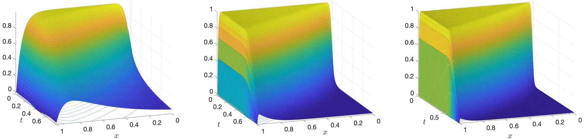\end{matrix} \end{matrix}$ Remark that $\partial_{w} erf (\frac{w}{g (t)}) = \frac{2}{\sqrt{π}} \frac{e^{- \frac{w^{2}}{g (t)}}}{g (t)}$ so that $W_{w}^{0} (w, t) = \frac{y_{0} - v}{\sqrt{π}} \frac{e^{- \frac{w^{2}}{\sqrt{2 (e^{2 t} - 1)}}}}{\sqrt{2 (e^{2 t} - 1)}}$ . As an illustration, Fig. 2 depicts the function $P^{ε}$ in $Q_{T}$ for $ε = 10^{- 1}, 10^{- 2}, 5 \times 10^{- 3}$ with $T = 0.8 > T_{0}$ . In particular, observe that $P^{ε}$ does not vanish at $x = 0$ and $x = 1$ but gets small as ε decreases. Table 1 provides some numerical values of the norm $‖ y^{ε} - P^{ε} ‖_{L^{\infty} (0, T; L^{2} (0, 1))}$ for several values of the parameter ε. The unknown solution $y^{ε}$ of (1) is obtained here using a numerical approximation. We obtain $‖ y^{ε} - P^{ε} ‖_{L^{\infty} (0, T; L^{2} (0, 1))} = O (ε^{0.61})$ in full agreement with our estimate in Theorem 3.1.

Fig. 2.

Function $P^{ε}$ given by (51) in $Q_{T}$ for $ε = 10^{- 1}, 10^{- 2}, 5 \times 10^{- 3}$ .

Table 1

$‖ y^{ε} - P^{ε} ‖_{L^{\infty} (0, T; L^{2} (0, 1))}$ w.r.t. ε for $T = 0.8$ , $y_{0} = 1$ and $v = 0$

ε	$10^{- 1}$	$5 \times 10^{- 2}$	$10^{- 2}$	$5 \times 10^{- 3}$	$10^{- 3}$
	$9.24 \times 10^{- 2}$	$6.14 \times 10^{- 2}$	$2.07 \times 10^{- 2}$	$1.4 \times 10^{- 2}$	$5.30 \times 10^{- 3}$

4.2. The case

M (x, t) = 1 + t

y_{0} (x) \equiv y_{0}

(0, 1)

v (t) \equiv v

(0, T)

In this case, the function $a (t)$ is given by $a (t) = \frac{t (t + 2)}{2}$ . $T_{0}$ such that $a (T_{0}) = 1$ is $T_{0} = \sqrt{3} - 1$ . Then, $\begin{matrix} α (t) : = M_{x} (a (t), t) = 0, β (t) : = e^{\int_{0}^{t} α (s) d s} = 1 B (t) : = \int_{0}^{t} \frac{1}{β {(s)}^{2}} d s = t, \end{matrix}$ leading to $β (t) \sqrt{B (t)} = \sqrt{t}$ . We obtain that $y^{0}$ defined by (7) is given by $\begin{matrix} y^{0} (x, t) = \{\begin{matrix} y_{0}, & x > \frac{t (t + 2)}{2}, \\ v, & x < \frac{t (t + 2)}{2}, \end{matrix} \end{matrix}$ and $\begin{matrix} W^{0} (w, t) = \frac{y_{0} - v}{2} erf (\frac{w}{2 \sqrt{t}}) + \frac{y_{0} + v}{2}, W^{1 / 2} (w, t) = 0, w = \frac{2 x - t (t + 2)}{2 ε^{1 / 2}} . \end{matrix}$ $p^{0}$ defined by (24) is given by $p^{0} (x, t) = W^{0} (w, t)$ while simply $p^{1 / 2} (x, t) = 0$ . Then, we get $\begin{matrix} C_{0} (τ, t) = W^{0} (2 τ, t), C_{1 / 2} (z, τ, t) = - z W_{w}^{0} (2 τ, t), z = \frac{1 - x}{ε}, τ = \frac{\sqrt{3} - 1 - t}{ε^{1 / 2}}, \end{matrix}$ implying $\begin{matrix} P^{0} (x, t) = W^{0} (w, t) - W^{0} (1 + t) τ, t) e^{- (1 + t) z}, P^{1 / 2} (x, t) = - z e^{- (1 + t) z} W_{w}^{0} ((1 + t) τ, t) . \end{matrix}$ Consequently, our approximation is given by $\begin{matrix} P^{ε} (x, t) = W^{0} (w, t) - W^{0} ((1 + t) τ, t) e^{- (1 + t) z} - ε^{1 / 2} z e^{- (1 + t) z} W_{w}^{0} ((1 + t) τ, t), \\ w = \frac{2 x - t (t + 2)}{2 ε^{1 / 2}}, z = \frac{1 - x}{ε}, τ = \frac{\sqrt{3} - 1 - t}{ε^{1 / 2}}, \end{matrix}$ with here $W_{w}^{0} (w, t) = \frac{y_{0} - v}{\sqrt{π}} \frac{e^{- \frac{w^{2}}{2 \sqrt{t}}}}{2 \sqrt{t}}$ .

5. Concluding remarks

We have performed an asymptotic analysis of the solution of an advection–diffusion equation with a small diffusion coefficient $ε > 0$ . The analysis takes into account the intersection of several singular layers and leads to an approximation in an $ε^{1 / 2}$ -neighborhood of the solution for the norm $L^{\infty} (0, T; L^{2} (0, 1))$ . This analysis extends [3] to non constant, strictly positive transport velocity, leading to much more technical arguments. In particular, the solution in the internal layer (following the characteristic starting form $(0, 0)$ ) solves a parabolic equation with non constant and unbounded coefficients related to the first derivatives of the velocity. The resulting solution is expressed in term of the kernel of the heat equation.

The $ε^{1 / 2}$ rate obtained for the final estimate is driven by our approximation $W^{0}$ in the internal layer, which depends on the non-unique choice of the function $g_{0}$ . The choice (19) is simple and involves the property ${lim}_{x \to 0^{+}} W^{0} (\frac{x}{ε^{1 / 2}}, 0) = y_{0} (0)$ in agreement with the fact that ${lim}_{x \to 0^{+}} y^{ϵ} (x, 0) = y_{0} (0)$ . However, it implies that ${lim}_{t \to 0^{+}} W^{0} (\frac{- a (t)}{ε^{1 / 2}}, t) = (y_{0} (0) + v (0)) / 2$ different for ${lim}_{t \to 0^{+}} y^{ε} (0, t) = v (0)$ when $y_{0} (0) \neq v (0)$ . This gap at the point $(0, 0)$ between $(y_{0} (0) + v (0)) / 2$ and $v (0)$ generates an artificial corner layer in the approximation in the neighborhood of the point $(0, 0)$ . This induces an error propagating along the characteristic $x - a (t) = 0$ then affects the quality of the approximation. Precisely, with this simple choice of $g_{0}$ , the $L^{1} (0, T)$ norms of $(W^{0} (\frac{- a (t)}{ε^{1 / 2}}, t) - v (0))$ and $\partial_{t} (W^{0} (\frac{- a (t)}{ε^{1 / 2}}, t) - v (0))$ are of order ε and one respectively (we refer to the proof of Lemma 3.6); this implies an approximation error of order $ε^{1 / 2}$ . By analogy with [3, Section 3] devoted to the constant transport case, one may consider the more involved choice $\begin{matrix} (52) & g_{0}^{ε} (w) : = \{\begin{matrix} y_{0} (0), & w ⩾ 0, \\ v (0) + \frac{v (0) - y_{0} (0)}{2} e^{\frac{F w}{ε^{1 / 2}}}, & w < 0, \end{matrix} \end{matrix}$ with $F : = {lim}_{t \to 0^{+}} \frac{a (t)}{β (t) B (t)} = a^{'} (0) > 0$ leading to $W_{ε}^{0} : = W^{0} + U_{ε}^{0}$ with $\begin{matrix} U_{ε}^{0} (w, t) = \frac{v (0) - y_{0} (0)}{2} e^{\frac{F w}{β (t) ε^{1 / 2}} + \frac{F^{2} B (t)}{ε}} erfc (\frac{w}{2 \sqrt{B (t)} β (t)} + \frac{F \sqrt{B (t)}}{ε^{1 / 2}}), \end{matrix}$ and $W^{0}$ defined by (20). The new function $W_{ε}^{0}$ still satisfies the asymptotic conditions ${lim}_{w \to + \infty} W_{ε}^{0} (w, t) = y_{0} (0)$ and ${lim}_{w \to - \infty} W_{ε}^{0} (w, t) = v (0)$ for all $t \in (0, T)$ . Moreover, we now observe that $\begin{matrix} lim_{t \to 0^{+}} W_{0}^{ε} (\frac{- a (t)}{ε^{1 / 2}}, t) = v (0), lim_{x \to 0^{+}} W_{ε}^{0} (\frac{x}{ε^{1 / 2}}, 0) = y_{0} (0) . \end{matrix}$ Therefore, this avoids at the first order the corner layer at the point $(0, 0)$ and allows to describe more accurately the discontinuity between the initial and Dirichlet conditions in the neighborhood of the point $(0, 0)$ . In [3] devoted to the constant transport case, this choice leads to an approximation error of order $O (ε^{3 / 4})$ . It remains to check that the choice (52) leads to the same rate in the non constant case.

Beyond this delicate issue related to the corner layer at the point $(0, 0)$ , in order to get a better rate, one would needs as in [3] to consider additional terms in the developments, notably the outer term $y^{1}$ defined in Section 2.2 not used here, internal layer terms $W^{1}$ , $W^{3 / 2}$ involving the heat kernel and boundary layer terms $Y^{1}$ and $Y^{3 / 2}$ solutions of ordinary differential equations with respect to the variable z. Whether or not we can perform the computations and get a priori estimates with these additional terms is an open issue.

In a future work we plan to study the parabolic system describing the miscible displacement of compressible fluids in a porous medium. The displacement of one compressible fluid by another, completely miscible with the first, in a one-dimensional porous medium $Ω = (0, 1)$ , assuming for simplicity that the two fluids have the same compressibility factor z, is described by the following differential system, see for instance [6], $\begin{array}{l} (53) & z \partial_{t} p + \partial_{x} q = 0, q = - \frac{κ}{μ (c)} \partial_{x} p, (x, t) \in Q_{T}, \\ (54) & ϕ \partial_{t} c + q (x, t) \partial_{x} c - \partial_{x} (d (x, t) \partial_{x} c)) = 0, (x, t) \in Q_{T}, \end{array}$ to which initial and boundary conditions are added. The unknowns of system (53), (54) are the functions $p = p (x, t)$ , $c = c (x, t)$ and $q = q (x, t)$ ; p is the pressure, c is the concentration of one of the two components of the fluid mixture, and q is the Darcy velocity. The function $κ = κ (x)$ is the permeability of the medium, the constant ϕ is the porosity, $μ = μ (c)$ is the concentration-dependent viscosity of the fluid mixture, $d = d (x, t)$ is a small term representing the molecular diffusion and dispersion in the porous medium. The viscosity $μ (c)$ is assumed to be determined by some mixing rule. See [4] for the existence of a weak solution to the one-dimensional equations governing compressible flows of m miscible components in a porous medium. Our aim is to perform an asymptotic analysis of system (53), (54) when d is small and the concentration c satisfies Dirichlet boundary conditions on $x = 0$ and $x = 1$ .

Footnotes

Acknowledgement

The authors thank the funding by the French government research program “Investissements d’Avenir” through the IDEX-ISITE initiative 16-IDEX-0001 (CAP 20-25).

Appendix

References

Amirat and

Münch, Asymptotic analysis of an advection–diffusion equation and application to boundary controllability, Asymptot. Anal. 112(1–2) (2019), 59–106.

Amirat and

Münch, On the controllability of an advection–diffusion equation with respect to the diffusion parameter: Asymptotic analysis and numerical simulations, Acta Math. Appl. Sin. Engl. Ser. 35(1) (2019), 54–110. doi:10.1007/s10255-019-0798-6.

Amirat and

Münch, Asymptotic analysis of an advection–diffusion equation involving interacting boundary and internal layers, Math. Methods Appl. Sci. 43(11) (2020), 6823–6860. doi:10.1002/mma.6425.

Amirat and

Shelukhin, Global weak solutions to equations of compressible miscible flows in porous media, SIAM J. Math. Anal. 38(6) (2007), 1825–1846. doi:10.1137/050640321.

D.G.

Aronson and

Besala, Parabolic equations with unbounded coefficients, J. Differential Equations 3 (1967), 1–14. doi:10.1016/0022-0396(67)90002-2.

Bear and

Bachmat, Introduction to Modeling of Transport Phenomena in Porous Media, Springer, Netherlands, 1990, p. XXIV+554. ISBN 9780792305576. doi:10.1007/978-94-009-1926-6.

Bodanko, Sur le problème de Cauchy et les problèmes de Fourier pour les équations paraboliques dans un domaine non borné, Ann. Polon. Math. 18 (1966), 79–94. doi:10.4064/ap-18-1-79-94.

Cheng,

Temam and

Wang, New approximation algorithms for a class of partial differential equations displaying boundary layer behavior, Methods Appl. Anal. 7(2) (2000), 363–390, Cathleen Morawetz: A great mathematician. doi:10.4310/MAA.2000.v7.n2.a6.

J.-M.

Coron and

Guerrero, Singular optimal control: A linear 1-D parabolic–hyperbolic example, Asymptot. Anal. 44(3–4) (2005), 237–257.

10.

Deuring,

Eymard and

Mildner,

L^{2}

-stability independent of diffusion for a finite element-finite volume discretization of a linear convection–diffusion equation, SIAM J. Numer. Anal. 53(1) (2015), 508–526. doi:10.1137/140961146.

11.

Eckhaus, Asymptotic Analysis of Singular Perturbations, Studies in Mathematics and Its Applications, Vol. 9, North-Holland Publishing Co., Amsterdam–New York, 1979, p. xi+287. ISBN 0-444-85306-5. doi:10.1016/S0168-2024(08)70012-2.

12.

Friedman, Partial Differential Equations of Parabolic Type, Prentice-Hall, Inc., Englewood Cliffs, N.J., 1964, p. xiv+347.

13.

G.-M.

Gie,

Hamouda,

C.-Y.

Jung and

R.M.

Temam, Singular Perturbations and Boundary Layers, Applied Mathematical Sciences, Vol. 200, Springer, Cham, 2018, p. xviii+412. ISBN 978-3-030-00637-2; 978-3-030-00638-9. doi:10.1007/978-3-030-00638-9.

14.

Guerrero and

Lebeau, Singular optimal control for a transport–diffusion equation, Comm. Partial Differential Equations 32(10–12) (2007), 1813–1836. doi:10.1080/03605300701743756.

15.

A.M.

Ilin, On the asymptotic behavior of the solution of a problem with a small parameter, Izv. Akad. Nauk SSSR Ser. Mat. 53(2) (1989), 258–275.

16.

A.M.

Ilin, Matching of Asymptotic Expansions of Solutions of Boundary Value Problems, Translations of Mathematical Monographs, Vol. 102, American Mathematical Society, Providence, RI, 1992, p. x+281, Translated from the Russian by V. Minachin [V.V. Minakhin]. ISBN 0-8218-4561-6. doi:10.1090/mmono/102.

17.

A.M.

Ilin,

A.S.

Kalašnikov and

O.A.

Oleĭnik, Second-order linear equations of parabolic type, Uspehi Mat. Nauk 17(3) (1962), 3–146.

18.

Kevorkian and

J.D.

Cole, Multiple Scale and Singular Perturbation Methods, Applied Mathematical Sciences, Vol. 114, Springer-Verlag, New York, 1996, p. viii+632. ISBN 0-387-94202-5. doi:10.1007/978-1-4612-3968-0.

19.

Laurent and

Léautaud, On uniform observability of gradient flows in the vanishing viscosity limit, J. Éc. polytech. Math. 8 (2021), 439–506. doi:10.5802/jep.151.

20.

Laurent and

Léautaud, On uniform controllability of 1D transport equations in the vanishing viscosity limit, C. R. Math. Acad. Sci. Paris 361 (2023), 265–312. doi:10.5802/crmath.405.

21.

Plaschko, Matched asymptotic approximations to solutions of a class of singular parabolic differential equations, Z. Angew. Math. Mech. 70(1) (1990), 63–64. doi:10.1002/zamm.19900700119.

22.

Sanchez Hubert and

Sánchez-Palencia, Vibration and Coupling of Continuous Systems: Asymptotic Methods, Springer-Verlag, Berlin, 1989, p. xvi+421. ISBN 3-540-19384-7. doi:10.1007/978-3-642-73782-4.

23.

Shao and

Meng, Gronwall–Bellman type inequalities and their applications to fractional differential equations, Abstr. Appl. Anal. 2013 (2013), Art. ID 217641, 7. doi:10.1155/2013/217641.

24.

Shao, Asymptotic analysis and domain decomposition for a singularly perturbed reaction–convection–diffusion system with shock–interior layer interactions, Nonlinear Anal. 66(2) (2007), 271–287. doi:10.1016/j.na.2005.11.024.

25.

S.-D.

Shih, A novel uniform expansion for a singularly perturbed parabolic problem with corner singularity, Methods Appl. Anal. 3(2) (1996), 203–227. doi:10.4310/MAA.1996.v3.n2.a3.

26.

S.-D.

Shih, On a class of singularly perturbed parabolic equations, ZAMM Z. Angew. Math. Mech. 81(5) (2001), 337–345. doi:10.1002/1521-4001(200105)81:5<337::AID-ZAMM337>3.0.CO;2-9.

27.

Stynes and

O’Riordan, Uniformly convergent difference schemes for singularly perturbed parabolic diffusion–convection problems without turning points, Numer. Math. 55(5) (1989), 521–544. doi:10.1007/BF01398914.

28.

Van Dyke, Perturbation Methods in Fluid Mechanics, annotated edn, The Parabolic Press, Stanford, Calif., 1975.

Internal layer intersecting the boundary of a domain in a singular advection–diffusion equation

Abstract

Keywords

1. Introduction. Problem statement

2.1. A property of the characteristics

2.2. Outer expansion

2.3. Inner expansion along the characteristic x − a ( t ) = 0

2.4. Representation of the functions W 0 and W 1 / 2

2.4.1. Fundamental solutions

2.4.3. Integral representation of W 1 / 2

Proposition 2.1. Assume that v ∈ C 1 ( [ 0 , T ] ) and y 0 ∈ C 1 ( [ 0 , 1 ] ) . Then p ε belongs to C 1 ( [ 0 , 1 ] × ( 0 , T ] ) . 2.6. Inner expansion along x = 1

2.7. Asymptotic composite approximation in Q T

3. Convergence of the sequence ( P ε ) ( ε > 0 )

3.1.1. Estimate of the initial layer corrector θ ε

4. Some explicit examples

4.1. The case M ( x , t ) = 1 + x , y 0 ( x ) ≡ y 0 in ( 0 , 1 ) , v ( t ) ≡ v in ( 0 , T )

5. Concluding remarks

Footnotes

Acknowledgement

Appendix

References

2.3. Inner expansion along the characteristic $x - a (t) = 0$

2.4. Representation of the functions $W^{0}$ and $W^{1 / 2}$

2.4.3. Integral representation of $W^{1 / 2}$

Proposition 2.1.
Assume that $v \in C^{1} ([0, T])$ and $y_{0} \in C^{1} ([0, 1])$ . Then $p^{ε}$ belongs to $C^{1} ([0, 1] \times (0, T])$ .

2.6. Inner expansion along $x = 1$

2.7. Asymptotic composite approximation in $Q_{T}$

3. Convergence of the sequence ${(P^{ε})}_{(ε > 0)}$

3.1.1. Estimate of the initial layer corrector $θ^{ε}$

4.1. The case $M (x, t) = 1 + x$ , $y_{0} (x) \equiv y_{0}$ in $(0, 1)$ , $v (t) \equiv v$ in $(0, T)$