Homogenization of an eigenvalue problem through rough surfaces

Abstract

In a bounded cylinder with a rough interface we study the asymptotic behaviour of the spectrum and its associated eigenspaces for a stationary heat propagation problem. The main novelty concerns the proof of the uniform a priori estimates for the eigenvalues. In fact, due to the peculiar geometry of the domain, standard techniques do not apply and a suitable new approach is developed.

Keywords

Eigenvalue problem homogenization rough surfaces interface conditions

1. Introduction

The homogenization of spectral problems in materials with very fine microstructure is an important and often complex problem. The pioneer work on this topic goes back to [4] where L. Boccardo and P. Marcellini characterize the homogenization of eigenvalues and eigenspaces in terms of G-convergence for equi-uniformly elliptic variational operators. The first results in presence of rapidly oscillating periodic coefficients in fixed domains were obtained later on by S. Kesavan in [22]. Successively, in [24], M. Vanninathan considers periodically perforated domains with Dirichlet, Neumann and Steklov boundary conditions. Then, general perforated domains were treated by M. Briane, A. Damlamian and P. Donato in [7], via $H^{0}$ convergence. Starting from these milestones, the homogenization of elliptic spectral problems for various kinds of domains has been object of several studies. In this article, we are concerned with composites presenting a rough interface.

Mathematical models involving boundary-value problems in domains with rough boundaries or surfaces are nowadays widely used to describe large classes of phenomena arising from engineering and material sciences applications. For instance, obstacles or medium fluctuations of small dimensions can modify acoustic wave propagation in inhomogeneous media. As an illustrating example, the sea-surface height can be measured by the time it takes for radar pulses to hit the ocean surface and bounce back to the spacecraft [2]. One can also think of the lubrication of rough surfaces [23], the frictional forces at the contact area of two different materials [8] (see also [19]), the turbulence flow over rough walls [1,21] and the heat and mass transfer on surfaces with roughness elements between solid and fluid interfaces [20].

This paper aims to examine the limit behaviour of the spectrum and its associated eigenspaces for a stationary heat propagation problem set in a composite with two connected components separated by a rough surface. This interface induces an imperfect contact between the two components. As observed in [9], such physical phenomenon is characterized by a jump of the temperature which is proportional to the heat flux across the interface.

For ease of presentation, we model the composite as an open and bounded cylinder $Q = ω \times] - ℓ, ℓ [$ in $R^{N}$ , $N ⩾ 2$ , where ω is a bounded smooth domain in $R^{N - 1}$ and $ℓ > 0$ , but more general domains can be considered, see Section 2 for details.

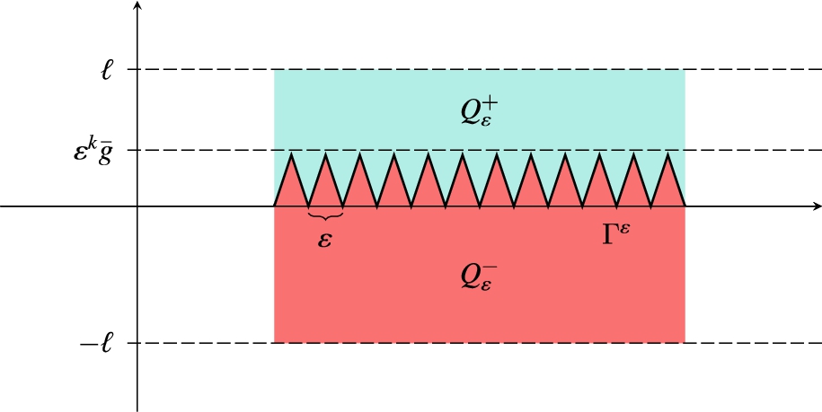
Given a small positive parameter ε, the rough interface $Γ^{ε}$ separating the two components is represented by the graph of a quickly oscillating function, ε-periodic in the first $N - 1$ variables. For instance, a possible configuration is given by the “saw-tooth” interface in Fig. 1. The amplitude of the oscillations is of order $ε^{k}$ , with $k > 0$ , therefore as $ε \to 0$ the interface approaches a flat surface $Γ_{0}$ , cf. Fig. 2.

In this context, we prescribe the proportionality in the interfacial condition to be of order $ε^{γ}$ , for $γ \in R$ . Furthermore, we assume that the thermal conductivity coefficient $A^{ε}$ is also ε-periodic rapidly oscillatory. Thus, we are concerned on the limit behaviour, as $ε \to 0$ , of the eigenvalues $λ^{ε}$ and the associated eigenfunctions $u_{ε}$ for the following problem: $\begin{matrix} (1.1) & \{\begin{array}{ll} - div (A^{ε} \nabla u_{ε}) = λ^{ε} u_{ε} & in Q ∖ Γ^{ε}, \\ {(A^{ε} \nabla u_{ε})}^{+} \cdot n_{ε} = {(A^{ε} \nabla u_{ε})}^{-} \cdot n_{ε} & on Γ^{ε}, \\ {(A^{ε} \nabla u_{ε})}^{+} \cdot n_{ε} = - ε^{γ} h^{ε} (u_{ε}^{+} - u_{ε}^{-}) & on Γ^{ε}, \\ u_{ε} = 0 & on \partial Q, \end{array} \end{matrix}$ where $h^{ε}$ is a positive bounded ε-periodic function in $R^{N - 1}$ and $n_{ε}$ is a unit normal to $Γ^{ε}$ .

Domains with rough interfaces in the vicinity of a hyperplane as in (1.1) were introduced by P. Donato and A. Piatnitski in [18] within the study of the homogenization of an elliptic boundary value problem. Later on, in [16], P. Donato and D. Giachetti considered the same problem with an additional singular lower order term. The analogous parabolic problem has been studied by P. Donato, E. Jose and D. Onofrei in [17] where the authors give a physical application of the problem as an alternative strategy for controlling the heat transfer in microstructures separated by a rough surface through an efficient design of the interface. The above mentioned articles show that the interfacial condition gives rise to different limit behaviours according to the amplitude of the oscillations k and the parameter γ. In [18] it is proved that these behaviours can be essentially subdivided into three main types, as described in Theorem 4.1 of Section 4. In case A), the limit problem is the classical homogenized elliptic Dirichlet one obtained for a composite without interface posed in the whole cylinder Q. In cases B) and C), the limit domain consists of two connected components separated by the flat interface $Γ_{0}$ . As for the limit problems, in case B), the homogenized diffusion equation presents an effective imperfect transmission condition modeled by a jump of the solution proportional to the flux on $Γ_{0}$ . Meanwhile, in case C), one obtains two independent homogenized elliptic problems posed in the two components of the limit domain, with Neumann boundary conditions on $Γ_{0}$ .

In the present work, once introduced the setting of the problem in Section 2, we first analyze the spectrum of the ε-problem (1.1) and its corresponding eigenspaces, see Section 3. Then, in Section 5, we characterize the eigenvalues associated with the limit problems given in Section 4. Finally, the a priori bounds detailed in Section 6 allow us to prove our main result in Section 7. More precisely, in Theorem 7.2 we show that the whole sequences of eigenvalues at level ε converge to the corresponding eigenvalues of the homogenized problems. The same convergence result is achieved for the corresponding eigenspaces. Furthermore, if an homogenized eigenvalue is simple, we get the convergence of the eigenfunctions for the whole sequence.

The main novelty arising in our study concerns the proof of the uniform a priori estimates for the eigenvalues of problem (1.1), stated in Proposition 6.3. A standard strategy in the literature is to estimate the eigenvalues of the ε-problems by means of the eigenvalues associated to the homogenized one. This can be done if the space generated by the eigenfunctions associated with the homogenized problem is contained in the space where the ε-problem eigenfunctions live. However, in our framework this technique only applies in case A). On the contrary, in cases B) and C), the necessary space inclusion does not hold, this renders the situation more complicated. To overcome this obstacle, we construct an appropriate space using a new different approach. This space, cf. (6.2) for the definition, is generated by the extensions by reflection of the eigenfunctions of an auxiliary eigenvalue problem set only in one of the components of the limit domain. The properties of the reflection, together with suitable technical tools given in Lemma 6.2, allow us to obtain the desired a priori estimates, via the eigenvalues of the auxiliary problem.

The homogenization of a similar eigenvalue problem posed in a different two-component domain has been recently considered in the work [15] by P. Donato, E. Gemida and E. Jose. In [10], G. Chechkin, A. Friedman and A. Piatnitski study the homogenization of a related elliptic problem with a nonhomogeneous Fourier boundary condition in domains with locally periodic highly oscillating boundaries.

2. Statement of the problem

We start with the geometric setting, originally introduced by P. Donato and A. Piatnitski in [18].

For $N ⩾ 2$ , we denote by

$Q = ω \times] - ℓ, ℓ [$ an open and bounded cylinder in $R^{N}$ , where ω is a bounded smooth domain in $R^{N - 1}$ and ℓ is a positive number,

$\tilde{v}$ the zero extension to the whole of Q of a function v defined on a subset of Q,

$Y =] 0, 1 [^{N}$ the volume reference cell,

$Y^{'} =] 0, 1 [^{N - 1}$ the surface reference cell,

$m_{E} (v)$ the average on E of a function $v \in L^{1} (E)$ , where E is an open subset of $R^{N - 1}$ or $R^{N}$ ,

$χ_{E}$ the characteristic function of a subset E of $R^{N}$ .

In order to describe the structure of the domain Q with rough interface $Γ^{ε}$ we consider a function g satisfying the hypothesis below.

H₁) The function $g : Y^{'} \to R$ is positive $Y^{'}$ -periodic and Lipschitz-continuous.

Given a positive real parameter ε converging to zero and $k > 0$ , we set $\begin{matrix} Γ^{ε} = {x \in Q | x_{N} = ε^{k} g (\frac{x^{'}}{ε})} \end{matrix}$ where $x^{'} = (x_{1}, \dots, x_{N - 1})$ .

Thus, the graph $Γ^{ε}$ divides the set Q in its upper part $\begin{matrix} Q_{ε}^{+} = {x \in Q | x_{N} > ε^{k} g (\frac{x^{'}}{ε})} \end{matrix}$ and its lower part $\begin{matrix} Q_{ε}^{-} = {x \in Q | x_{N} < ε^{k} g (\frac{x^{'}}{ε})} . \end{matrix}$ If we set $\bar{g} = max g$ , then, by construction, the cylinder $ω \times [0, ε^{k} \bar{g}]$ contains the oscillating surface and its measure goes to zero as ε approaches zero.

A possible configuration of this type of domain is given in Fig. 1.

Fig. 1.

The domain Q with oscillating interface $Γ^{ε}$ .

As observed in [18], one can consider a more general smooth domain Q such that for any point of $\partial Q \cap {x ∣ x_{N} = 0}$ the normal to $\partial Q$ is not parallel to the N-th coordinate vector.

Remark 2.1.

The case $k = 1$ presents a self-similar geometry because the interface $Γ^{ε}$ can be obtained by a homothetic dilatation of the fixed function $y_{N} = g (y^{'})$ in $R^{N}$ . The case $k > 1$ represents the flat case, while the case $0 < k < 1$ describes a highly oscillating interface.

In this setting, we are concerned on the limit behaviour, as $ε \to 0$ , of the following eigenvalue problem: $\begin{matrix} (2.1) & \{\begin{array}{ll} - div (A^{ε} \nabla u_{ε}) = λ^{ε} u_{ε} & in Q ∖ Γ^{ε}, \\ {(A^{ε} \nabla u_{ε})}^{+} \cdot n_{ε} = {(A^{ε} \nabla u_{ε})}^{-} \cdot n_{ε} & on Γ^{ε}, \\ {(A^{ε} \nabla u_{ε})}^{+} \cdot n_{ε} = - ε^{γ} h^{ε} (u_{ε}^{+} - u_{ε}^{-}) & on Γ^{ε}, \\ u_{ε} = 0 & on \partial Q, \end{array} \end{matrix}$ where $n_{ε}$ is the unit outward normal to $Q_{ε}^{+}$ .

For the coefficients of problem (2.1), we assume the following hypotheses:

H₂) For any $ε > 0$ , $A^{ε} (x) = A (\frac{x}{ε})$ where A is a Y-periodic symmetric matrix field satisfying $\begin{matrix} (A (y) λ, λ) ⩾ α | λ |^{2}, | A (y) λ | ⩽ β | λ |, \forall λ \in R^{N} and a.e. in Y, \end{matrix}$ with $α, β \in R$ , $0 < α < β$ .

H₃) For any $ε > 0$ , $h^{ε} (x^{'}) = h (\frac{x^{'}}{ε})$ where h is a $Y^{'}$ -periodic function in $L^{\infty} (Γ)$ , with $Γ = {y_{N} = g (y^{'}), y^{'} \in Y^{'}}$ , such that there exists $h_{0} \in R : 0 < h_{0} < h (y^{'}) a.e. on Γ$ .

Let us establish the functional framework. For any function v defined on Q, we set $\begin{matrix} v_{ε}^{+} = v_{| Q_{ε}^{+}} and v_{ε}^{-} = v_{| Q_{ε}^{-}} . \end{matrix}$ We define the Hilbert space $\begin{matrix} W_{0}^{ε} = {v \in L^{2} (Q) ∣ v_{ε}^{+} \in H^{1} (Q_{ε}^{+}), v_{ε}^{-} \in H^{1} (Q_{ε}^{-}), v = 0 on \partial Q}, \end{matrix}$ equipped with the norm $\begin{matrix} (2.2) & ‖ v ‖_{W_{0}^{ε}} = ‖ \nabla v ‖_{L^{2} (Q ∖ Γ^{ε})} \end{matrix}$ where $\nabla v = \tilde{\nabla v_{ε}^{+}} + \tilde{\nabla v_{ε}^{-}}$ . That is, we identify $\nabla v$ with the absolutely continuous part of the gradient of v. The left-hand side of (2.2) is a norm as a consequence of the Poincaré inequality. In particular, we remark that the positive constant C such that for any $v \in W_{0}^{ε}$ $\begin{matrix} ‖ v ‖_{L^{2} (Q)} ⩽ C ‖ \nabla v ‖_{L^{2} (Q ∖ Γ^{ε})} \end{matrix}$ is independent of ε.

For the space $W_{0}^{ε}$ one has the following compactness results, proved in [18]:

Proposition 2.2 ([18]).

Suppose ${v_{ε}}$ is a family of functions in $W_{0}^{ε}$ such that $\begin{matrix} ‖ v_{ε} ‖_{W_{0}^{ε}} ⩽ C, \end{matrix}$ with C positive constant independent of ε. Then, the family ${v_{ε}}$ is compact in $L^{2} (Q)$ and the families ${χ_{Q_{ε}^{+}} \nabla v_{ε}}$ and ${χ_{Q_{ε}^{-}} \nabla v_{ε}}$ are weakly compact in $L^{2} (Q)$ .

The variational formulation of problem (2.1) then reads as $\begin{matrix} (2.3) & \{\begin{array}{l} Find (λ^{ε}, u_{ε}) \in R \times [W_{0}^{ε} ∖ {0}] such that \\ \int_{Q ∖ Γ^{ε}} A^{ε} \nabla u_{ε} \nabla v d x + ε^{γ} \int_{Γ^{ε}} h^{ε} (u_{ε}^{+} - u_{ε}^{-}) (v_{ε}^{+} - v_{ε}^{-}) d σ = λ^{ε} \int_{Q} u_{ε} v d x, \\ for all v \in W_{0}^{ε} . \end{array} \end{matrix}$

Remark 2.3.
By virtue of Lax–Milgram theorem, $λ^{ε}$ cannot be zero as in this case the only solution of the homogeneous problem (2.3) is $u_{ε} = 0$ , which is not an eigenfunction.
3. Eigenvalues and eigenfunctions for fixed $ε$

This section is devoted to the analysis of the spectrum of problem (2.1) and its associated eigenspaces. For the reader’s convenience, we recall well-known results holding for general symmetric operators as stated in [12] (see, for instance, [6] and [25] for a proof).

Theorem 3.1 ([12]).

Let $B : H \to H$ , $B ≢ 0$ , a linear, compact, symmetric operator on the real infinite-dimensional Hilbert space H such that $B u = 0$ implies $u = 0$ . Then, the following hold true:

The set of eigenvalues of $B$ is a countable set of $R^{+}$ whose unique accumulation point is zero.

Every eigenvalue is of finite multiplicity, that is, its corresponding eigenspace is a vector subspace of H of positive finite dimension.

Let ${ρ_{l}}$ be the sequence of the eigenvalues numbered in non-increasing order, where each eigenvalue is repeated as many times as the dimension of its corresponding eigenspace, that is $\begin{matrix} ρ_{1} ⩾ ρ_{2} ⩾ \dots \to 0 . \end{matrix}$ Then, there exists a corresponding sequence of eigenfunctions ${v_{l}}$ which forms a complete orthonormal system in H.

Using the previous theorem we prove the following result for our case:

Theorem 3.2.
Let ε be fixed. Suppose g, $A^{ε}$ and $h^{ε}$ satisfy assumptions H ₁ ), H ₂ ) and H ₃ ), respectively. Then,
The set of eigenvalues of problem ( 2.3 ) is a countable set of $R^{+}$ whose unique accumulation point is $+ \infty$ .

Every eigenvalue is of finite multiplicity, that is, its corresponding eigenspace is a vector subspace of $L^{2} (Q)$ of positive finite dimension.

Let ${λ_{l}^{ε}}$ be the sequence of the eigenvalues numbered in increasing order, where each eigenvalue is repeated as many times as the dimension of its corresponding eigenspace, that is $\begin{matrix} 0 < λ_{1}^{ε} ⩽ λ_{2}^{ε} ⩽ \dots \to + \infty . \end{matrix}$ Then, there exists a corresponding sequence of eigenfunctions ${u_{ε, l}}$ in $W_{0}^{ε}$ which forms a complete orthonormal system in $L^{2} (Q)$ .

Proof.
We use Theorem 3.1 with $B : L^{2} (Q) \to L^{2} (Q)$ defined as follows. Let $\begin{matrix} Ψ : f \in L^{2} (Q) \mapsto u_{f} \in W_{0}^{ε}, \end{matrix}$ where $u_{f}$ is the unique solution of problem $\begin{matrix} (3.1) & \{\begin{array}{l} Find u_{f} \in W_{0}^{ε} such that \\ \int_{Q ∖ Γ^{ε}} A^{ε} \nabla u_{f} \nabla v d x + ε^{γ} \int_{Γ^{ε}} h^{ε} ({u_{f}}_{ε}^{+} - {u_{f}}_{ε}^{-}) (v_{ε}^{+} - v_{ε}^{-}) d σ = \int_{Q} f v d x, \\ for all v \in W_{0}^{ε} . \end{array} \end{matrix}$ The Lax–Milgram theorem ensures the existence and uniqueness of the solution of problem (3.1). Moreover, one can easily obtain the following a priori estimate: $\begin{matrix} (3.2) & ‖ u_{f} ‖_{W_{0}^{ε}} + ε^{\frac{γ}{2}} {‖ {u_{f}}_{ε}^{+} - {u_{f}}_{ε}^{-} ‖}_{L^{2} (Γ^{ε})} ⩽ C ‖ f ‖_{L^{2} (Q)}, \end{matrix}$ for some positive constant C.

Now, let $\begin{matrix} B = i \circ Ψ : f \in L^{2} (Q) \mapsto u_{f} \in L^{2} (Q), \end{matrix}$ where i denotes the embedding of $W_{0}^{ε}$ in $L^{2} (Q)$ .

The linearity of $B$ is immediate.

To verify the compactness of $B$ , suppose ${f_{n}}$ is a bounded sequence in $L^{2} (Q)$ . By (3.2), $‖ u_{f_{n}} ‖_{W_{0}^{ε}} ⩽ C ‖ f_{n} ‖_{L^{2} (Q)}$ , so that ${Ψ (f_{n})}$ is bounded in $W_{0}^{ε}$ . Thus, ${i \circ Ψ (f_{n})}$ has a convergent subsequence in $L^{2} (Q)$ , since i is compact in view of Proposition 2.2.

The symmetry of A easily gives the one of $B$ , indeed $\begin{aligned} {⟨ B f, g ⟩}_{L^{2} (Q), L^{2} (Q)} & = \int_{Q} u_{f} g d x = \int_{Q} g u_{f} d x \\ = \int_{Q ∖ Γ^{ε}} A^{ε} \nabla u_{g} \nabla u_{f} d x + ε^{γ} \int_{Γ^{ε}} h^{ε} ({u_{g}}_{ε}^{+} - {u_{g}}_{ε}^{-}) ({u_{f}}_{ε}^{+} - {u_{f}}_{ε}^{-}) d σ \\ = \int_{Q ∖ Γ^{ε}} A^{ε} \nabla u_{f} \nabla u_{g} d x + ε^{γ} \int_{Γ^{ε}} h^{ε} ({u_{f}}_{ε}^{+} - {u_{f}}_{ε}^{-}) ({u_{g}}_{ε}^{+} - {u_{g}}_{ε}^{-}) d σ \\ = \int_{Q} f u_{g} d x = {⟨ f, B g ⟩}_{L^{2} (Q), L^{2} (Q)} . \end{aligned}$

Finally, if $B f = 0$ , then, by definition of $B$ , $u_{f} = 0$ . Thus, by uniqueness, $f = 0$ . Therefore, $B$ satisfies all the assumptions of Theorem 3.1.

Now observe that by i. of Theorem 3.1, the set of eigenvalues of the operator $B$ forms a sequence of positive real numbers converging to zero. Let ${ρ_{l}^{ε}}$ denote the sequence of these eigenvalues where each eigenvalue is repeated as many times as its multiplicity, numbered in non-increasing order. In view of $iii$ . of Theorem 3.1, there exists a corresponding sequence of eigenfunctions ${u_{ε, l}}$ (i.e., verifying $B u_{ε, l} = ρ_{l}^{ε} u_{ε, l}$ ) forming a complete orthonormal system in $L^{2} (Q)$ .

On the other hand, since by Remark 2.3 one has $λ_{l}^{ε} \neq 0$ , the identity $\begin{array}{c} \int_{Q ∖ Γ^{ε}} A^{ε} \nabla u_{ε, l} \nabla v d x + ε^{γ} \int_{Γ^{ε}} h^{ε} (u_{ε, l}^{+} - u_{ε, l}^{-}) (v_{ε}^{+} - v_{ε}^{-}) d σ = λ_{l}^{ε} \int_{Q} u_{ε, l} v d x \end{array}$ is equivalent to $\begin{array}{c} \int_{Q ∖ Γ^{ε}} A^{ε} \nabla (\frac{1}{λ_{l}^{ε}} u_{ε, l}) \nabla v d x + ε^{γ} \int_{Γ^{ε}} h^{ε} ((\frac{1}{λ_{l}^{ε}} u_{ε, l}^{+}) - (\frac{1}{λ_{l}^{ε}} u_{ε, l}^{-})) (v_{ε}^{+} - v_{ε}^{-}) d σ = \int_{Q} u_{ε, l} v d x . \end{array}$ Thus, $B u_{ε, l} = \frac{1}{λ_{l}^{ε}} u_{ε, l}$ . Therefore, for each $l \in N$ , $ρ_{l}^{ε} = \frac{1}{λ_{l}^{ε}}$ .

This implies that the eigenvalues $λ_{l}^{ε}$ form an increasing sequence that goes to infinity. □

Adapting to our case the classical min-max principle on the characterization of eigenvalues (see for instance [14]), we derive the next proposition. Proposition 3.3.
For fixed ε, let ${λ_{l}^{ε}}$ be the sequence of the eigenvalues of problem ( 2.3 ) and ${u_{ε, l}}$ be the corresponding sequence of eigenfunctions given in $iii$ . of Theorem 3.2 . Then, for each $l \in N$ , $\begin{aligned} (3.3) & λ_{l}^{ε} & = max_{\begin{array}{c} v \in V_{l}^{ε} \\ ‖ v ‖_{L^{2} (Q)} = 1 \end{array}} (\int_{Q ∖ Γ^{ε}} A^{ε} \nabla v \nabla v d x + ε^{γ} \int_{Γ^{ε}} h^{ε} {(v_{ε}^{+} - v_{ε}^{-})}^{2} d σ) \\ (3.4) & = min_{\begin{array}{c} v \in {(V_{l - 1}^{ε})}^{⊥} \\ ‖ v ‖_{L^{2} (Q)} = 1 \end{array}} (\int_{Q ∖ Γ^{ε}} A^{ε} \nabla v \nabla v d x + ε^{γ} \int_{Γ^{ε}} h^{ε} {(v_{ε}^{+} - v_{ε}^{-})}^{2} d σ) \\ (3.5) & = min_{M \in D_{l}^{ε}} max_{\begin{array}{c} v \in M \\ ‖ v ‖_{L^{2} (Q)} = 1 \end{array}} (\int_{Q ∖ Γ^{ε}} A^{ε} \nabla v \nabla v d x + ε^{γ} \int_{Γ^{ε}} h^{ε} {(v_{ε}^{+} - v_{ε}^{-})}^{2} d σ) \\ (3.6) & = max_{M \in D_{l - 1}^{ε}} min_{\begin{array}{c} v \in M^{⊥} \\ ‖ v ‖_{L^{2} (Q)} = 1 \end{array}} (\int_{Q ∖ Γ^{ε}} A^{ε} \nabla v \nabla v d x + ε^{γ} \int_{Γ^{ε}} h^{ε} {(v_{ε}^{+} - v_{ε}^{-})}^{2} d σ) \end{aligned}$ where $V_{l}^{ε} = span {u_{ε, 1}, \dots, u_{ε, l}}$ and $D_{l}^{ε} = {M \subset W_{0}^{ε} | dim M = l}$ .
Proof.
Let $v \in W_{0}^{ε}$ . Since the sequence ${u_{ε, l}}$ forms a complete orthonormal system in $L^{2} (Q)$ , one has $v = \sum_{k = 1}^{+ \infty} c_{k} u_{ε, k}$ , with $c_{k} = {⟨ u_{ε, k}, v ⟩}_{L^{2} (Q), L^{2} (Q)}$ . Moreover, if $‖ v ‖_{L^{2} (Q)} = 1$ then $\sum_{k = 1}^{+ \infty} | c_{k} |^{2} = 1$ .

Now, define the bilinear map $a : (u, v) \in W_{0}^{ε} \times W_{0}^{ε} \mapsto R$ as $\begin{matrix} a (u, v) = \int_{Q ∖ Γ^{ε}} A^{ε} \nabla u \nabla v d x + ε^{γ} \int_{Γ^{ε}} h^{ε} (u_{ε}^{+} - u_{ε}^{-}) (v_{ε}^{+} - v_{ε}^{-}) d σ . \end{matrix}$

One has $\begin{matrix} (3.7) & \begin{aligned} a (v, v) & = a (\sum_{i = 1}^{+ \infty} c_{i} u_{ε, i}, \sum_{j = 1}^{+ \infty} c_{j} u_{ε, j}) = \sum_{i, j = 1}^{+ \infty} c_{i} c_{j} a (u_{ε, i}, u_{ε, j}) \\ = \sum_{i, j = 1}^{+ \infty} c_{i} c_{j} λ_{i}^{ε} {⟨ u_{ε, i}, u_{ε, j} ⟩}_{L^{2} (Q), L^{2} (Q)} \\ = \sum_{i, j = 1}^{+ \infty} c_{i} c_{j} λ_{i}^{ε} δ_{i j} = \sum_{k = 1}^{+ \infty} | c_{k} |^{2} λ_{k}^{ε}, \end{aligned} \end{matrix}$ where $δ_{i j}$ is the Kronecker delta.

Let $V_{l}^{ε} = span {u_{ε, 1}, \dots, u_{ε, l}}$ . We first show (3.3). To this aim, let us start observing that for all $v \in V_{l}^{ε}$ such that $‖ v ‖_{L^{2} (Q)} = 1$ , one has $\sum_{k = 1}^{l} | c_{k} |^{2} = 1$ . Therefore, by $iii$ . of Theorem 3.2 and (3.7), one has $\begin{matrix} a (v, v) = \sum_{k = 1}^{l} | c_{k} |^{2} λ_{k}^{ε} ⩽ λ_{l}^{ε} \sum_{k = 1}^{l} | c_{k} |^{2} = λ_{l}^{ε} . \end{matrix}$ Moreover, $λ_{l}^{ε} = max_{\begin{array}{c} v \in V_{l}^{ε} \\ ‖ v ‖_{L^{2} (Q)} = 1 \end{array}} a (v, v)$ , indeed $\begin{matrix} (3.8) & \begin{aligned} a (\frac{u_{ε, l}}{‖ u_{ε, l} ‖_{L^{2} (Q)}}, \frac{u_{ε, l}}{‖ u_{ε, l} ‖_{L^{2} (Q)}}) & = \frac{1}{‖ u_{ε, l} ‖_{L^{2} (Q)}^{2}} a (u_{ε, l}, u_{ε, l}) \\ = \frac{1}{‖ u_{ε, l} ‖_{L^{2} (Q)}^{2}} λ_{l}^{ε} ‖ u_{ε, l} ‖_{L^{2} (Q)}^{2} = λ_{l}^{ε} . \end{aligned} \end{matrix}$

As for the characterization in (3.4), let $v \in {(V_{l - 1}^{ε})}^{⊥}$ be such that $‖ v ‖_{L^{2} (Q)} = 1$ . Then $\sum_{k = l}^{+ \infty} | c_{k} |^{2} = 1$ . From $iii$ . of Theorem 3.2 and (3.7) we have $\begin{matrix} a (v, v) = \sum_{k = l}^{+ \infty} | c_{k} |^{2} λ_{k}^{ε} ⩾ λ_{l}^{ε} \sum_{k = l}^{+ \infty} | c_{k} |^{2} = λ_{l}^{ε} . \end{matrix}$ Hence, $λ_{l}^{ε} = min_{\begin{array}{c} v \in {(V_{l - 1}^{ε})}^{⊥} \\ ‖ v ‖_{L^{2} (Q)} = 1 \end{array}} a (v, v)$ since, arguing as in (3.8), the minimum is attained at $v = \frac{u_{ε, l}}{‖ u_{ε, l} ‖_{L^{2} (Q)}}$ .

To prove (3.5), let $M \in D_{l}^{ε}$ and ${e_{1}, \dots, e_{l}}$ be a basis of M. Clearly, any $w \in M$ can be written as $w = \sum_{i = 1}^{l} d_{i} e_{i}$ , for some $d_{i} \in R$ , $i = 1, \dots, l$ . Now, we show that we can choose some constants $d_{i}$ , with at least one to be nonzero, such that w belongs also to ${(V_{l - 1}^{ε})}^{⊥}$ . Indeed, the system of equations $\begin{matrix} \sum_{i = 1}^{l} d_{i} {⟨ e_{i}, u_{ε, j} ⟩}_{L^{2} (Q), L^{2} (Q)} = 0, for j = 1, \dots, l - 1 \end{matrix}$ has $l - 1$ equations with l unknowns.

We can assume that the vector $w \in M \cap {(V_{l - 1}^{ε})}^{⊥} ∖ {0}$ has unitary norm, i.e. $‖ w ‖_{L^{2} (Q)}^{2} = \sum_{k = l}^{+ \infty} | c_{k} |^{2} = 1$ .

Then, $a (w, w) = \sum_{k = l}^{+ \infty} | c_{k} |^{2} λ_{k}^{ε} ⩾ λ_{l}^{ε}$ . Hence, $inf_{M \in D_{l}^{ε}} max_{\begin{array}{c} v \in M \\ ‖ v ‖_{L^{2} (Q)} = 1 \end{array}} a (v, v) ⩾ λ_{l}^{ε}$ . Finally, since $V_{l}^{ε} \in D_{l}^{ε}$ , using (3.3) we get $min_{M \in D_{l}^{ε}} max_{\begin{array}{c} v \in M \\ ‖ v ‖_{L^{2} (Q)} = 1 \end{array}} a (v, v) = λ_{l}^{ε}$ .

It remains to prove (3.6). Let $M \in D_{l - 1}^{ε}$ . Observe that there exists a function $w_{1} = \sum_{i = 1}^{l} k_{i} u_{ε, i} \in M^{⊥}$ . Indeed, for any basis ${ξ_{1}, \dots, ξ_{l - 1}}$ of M, the system of equations $\begin{matrix} \sum_{i = 1}^{l} k_{i} {⟨ u_{ε, i}, ξ_{j} ⟩}_{L^{2} (Q), L^{2} (Q)} = 0, for j = 1, \dots, l - 1 \end{matrix}$ has $l - 1$ equations with l unknowns. Thus, a nontrivial vector of coefficients $k_{i}$ , $i = 1, \dots, l$ , exists. We can choose $k_{i}$ such that $‖ w_{1} ‖_{L^{2} (Q)}^{2} = \sum_{k = 1}^{l} | k_{i} |^{2} = 1$ , then, $a (w_{1}, w_{1}) = \sum_{i = 1}^{l} | k_{i} |^{2} λ_{k}^{ε} ⩽ λ_{l}^{ε}$ . Hence, $sup_{M \in D_{l - 1}^{ε}} min_{\begin{array}{c} v \in M^{⊥} \\ ‖ v ‖_{L^{2} (Q)} = 1 \end{array}} a (v, v) ⩽ λ_{l}^{ε}$ . From (3.4), as before, we have $max_{M \in D_{l - 1}^{ε}} min_{\begin{array}{c} v \in M^{⊥} \\ ‖ v ‖_{L^{2} (Q)} = 1 \end{array}} a (v, v) = λ_{l}^{ε}$ , which completes the proof. □

4. Asymptotic behaviour of a related problem

To examine the limit behaviour of the spectrum and of the associated eigenspaces of problem (2.1), we have to deal with the homogenization of problem $\begin{matrix} (4.1) & \{\begin{array}{ll} - div (A^{ε} \nabla u_{ε}) = f^{ε} & in Q ∖ Γ^{ε}, \\ {(A^{ε} \nabla u_{ε})}^{+} \cdot n_{ε} = {(A^{ε} \nabla u_{ε})}^{-} \cdot n_{ε} & on Γ^{ε}, \\ {(A^{ε} \nabla u_{ε})}^{+} \cdot n_{ε} = - ε^{γ} h^{ε} (u_{ε}^{+} - u_{ε}^{-}) & on Γ^{ε}, \\ u_{ε} = 0 & on \partial Q, \end{array} \end{matrix}$ where the function g, the matrix $A^{ε}$ and the function $h^{ε}$ satisfy assumptions H₁), H₂), H₃), respectively, and $\begin{matrix} (4.2) & f^{ε} ⇀ f weakly in L^{2} (Q), \end{matrix}$ for some $f \in L^{2} (Q)$ .

To this aim, let us set $\begin{matrix} Q^{+} = {x \in Q ∣ x_{N} > 0}, Q^{-} = {x \in Q ∣ x_{N} < 0} and Γ_{0} = {x \in Q ∣ x_{N} = 0} \end{matrix}$ (see Fig. 2) and for any function v defined on Q, denote by $\begin{matrix} v^{+} = v_{| Q^{+}} and v^{-} = v_{| Q^{-}} . \end{matrix}$

We define the Hilbert space $W_{0}^{0}$ corresponding to the limit domain by $\begin{matrix} W_{0}^{0} = {v \in L^{2} (Q) ∣ v^{+} \in H^{1} (Q^{+}), v^{-} \in H^{1} (Q^{-}), v = 0 on \partial Q} \end{matrix}$ (see [18]).

Fig. 2.

The domain Q with flat interface $Γ_{0}$ .

We endow this space with the norm $\begin{matrix} ‖ v ‖_{W_{0}^{0}} = ‖ \nabla v ‖_{L^{2} (Q ∖ Γ_{0})}, where \nabla v = \tilde{\nabla v^{+}} + \tilde{\nabla v^{-}} . \end{matrix}$

The interfacial condition in the variational formulation of problem (4.1) gives rise to different limit behaviours according to the amplitude of the oscillations k and the parameter γ. However, the homogenized tensor $A^{0}$ is the same. Namely, it is the one obtained in [3] for the classical case of a fixed domain given by $\begin{matrix} (4.3) & A^{0} λ = m_{Y} (A \nabla w_{λ}), \end{matrix}$ with $w_{λ} \in H^{1} (Y)$ unique solution, for any $λ \in R^{N}$ , of $\begin{matrix} \{\begin{array}{ll} - div (A \nabla w_{λ}) = 0 & in Y, \\ w_{λ} - λ \cdot y & Y -periodic, \\ m_{Y} (w_{λ} - λ \cdot y) = 0 . \end{array} \end{matrix}$ It is renewed (see, for instance, [11,13]) that since the matrix A is symmetric the homogenized tensor $A^{0}$ defined in (4.3) is symmetric too. Moreover, $\begin{matrix} (4.4) & (A^{0} λ, λ) ⩾ α | λ |^{2} and | A^{0} λ | ⩽ β | λ |, \forall λ \in R^{N}, \end{matrix}$ with α and β given by hypothesis H₂).

The asymptotic behaviour, as $ε \to 0$ , of the solutions of (4.1) can be easily obtained arguing as in [18] where the right-hand side does not depend on ε. Therefore, we state the results without proof in the theorem below.

Theorem 4.1.

Under assumptions H ₁ ), H ₂ ), H ₃ ) and ( 4.2 ), let $u_{ε}$ be the solution of problem ( 4.1 ). Then there exists a function $u_{0} \in W_{0}^{0}$ such that $\begin{matrix} \{\begin{array}{ll} u_{ε} \to u_{0} & strongly in L^{2} (Q), \\ χ_{Q_{ε}^{+}} \nabla u_{ε} ⇀ χ_{Q^{+}} \nabla u_{0} & weakly in {(L^{2} (Q))}^{N}, \\ χ_{Q_{ε}^{-}} \nabla u_{ε} ⇀ χ_{Q^{-}} \nabla u_{0} & weakly in {(L^{2} (Q))}^{N} . \end{array} \end{matrix}$ Case A): ( $k ⩾ 1$ and $γ < 0$ ) or ( $0 < k < 1$ and $γ < 1 - k$ )

The limit function $u_{0}$ belongs to $H_{0}^{1} (Q)$ and it is the unique solution of problem $\begin{matrix} (4.5) & \{\begin{array}{ll} - div (A^{0} \nabla u_{0}) = f & in Q, \\ u_{0} = 0 & on \partial Q . \end{array} \end{matrix}$ Case B): ( $k ⩾ 1$ and $γ = 0$ ) or ( $0 < k < 1$ and $γ = 1 - k$ )

The limit function $u_{0} \in W_{0}^{0}$ is the unique solution of problem $\begin{matrix} (4.6) & \{\begin{array}{ll} - div (A^{0} \nabla u_{0}) = f & in Q ∖ Γ_{0}, \\ {(A^{0} \nabla u_{0})}^{+} \cdot n = {(A^{0} \nabla u_{0})}^{-} \cdot n & on Γ_{0}, \\ {(A^{0} \nabla u_{0})}^{+} \cdot n = - H (g, h) (u_{0}^{+} - u_{0}^{-}) & on Γ_{0}, \\ u_{0} = 0 & on \partial Q, \end{array} \end{matrix}$ where n is the unit outward normal to $Q^{+}$ and $\begin{matrix} (4.7) & H (g, h) = \{\begin{array}{ll} m_{Y^{'}} (h {(1 + | \nabla g |^{2})}^{\frac{1}{2}}) & if k = 1, γ = 0, \\ m_{Y^{'}} (h) & if k > 1, γ = 0, \\ m_{Y^{'}} (h | \nabla g |) & if 0 < k < 1, γ = 1 - k . \end{array} \end{matrix}$ Case C): ( $k ⩾ 1$ and $γ > 0$ ) or ( $0 < k < 1$ and $γ > 1 - k$ )

The limit function $u_{0} \in W_{0}^{0}$ is the unique solution of problem $\begin{matrix} (4.8) & \{\begin{array}{ll} - div (A^{0} \nabla u_{0}) = f & in Q ∖ Γ_{0}, \\ {(A^{0} \nabla u_{0})}^{+} \cdot n = {(A^{0} \nabla u_{0})}^{-} \cdot n = 0 & on Γ_{0}, \\ u_{0} = 0 & on \partial Q, \end{array} \end{matrix}$ where n is the unit outward normal to $Q^{+}$ .

This problem is equivalent to the following two (independent) Neumann problems solved by $u_{0}^{+}$ and $u_{0}^{-}$ , respectively: $\begin{matrix} \{\begin{array}{ll} - div (A^{0} \nabla u_{0}^{+}) = f & in Q^{+}, \\ (A^{0} \nabla u_{0}^{+}) \cdot n = 0 & on Γ_{0}, \\ u_{0}^{+} = 0 & on \partial Q^{+} ∖ Γ_{0}, \end{array} \end{matrix}$ and $\begin{matrix} \{\begin{array}{ll} - div (A^{0} \nabla u_{0}^{-}) = f & in Q^{-}, \\ (A^{0} \nabla u_{0}^{-}) \cdot n = 0 & on Γ_{0}, \\ u_{0}^{-} = 0 & on \partial Q^{-} ∖ Γ_{0} . \end{array} \end{matrix}$

Remark 4.2.

In case A), the presence of the interface is neglectful, the homogenized problem being the same obtained in [3] without any interface.

In case B), the result shows that the shape of g contributes in the limit problems only in the self-similar case $(k = 1)$ with $γ = 0$ and in the presence of the oscillating interface $(0 < k < 1)$ with $γ = 1 - k$ . While in the flat case, $(k > 1)$ with $γ = 0$ there is no difference, at the limit, if one replaces the oscillating interface with a flat one $Γ_{0}$ .

In case C), the theorem reveals that the problems in the two components are split at the limit and $Γ_{0}$ represents an isolating interface.

5. Eigenvalues and eigenfunctions of the limit problems

We consider here the eigenvalue problems associated with the limit problems (4.5), (4.6) and (4.8). Namely,

for case A): $\begin{matrix} (5.1) & \{\begin{array}{ll} - div (A^{0} \nabla u) = λ u & in Q, \\ u = 0 & on \partial Q; \end{array} \end{matrix}$ for case B): $\begin{matrix} (5.2) & \{\begin{array}{ll} - div (A^{0} \nabla u) = λ u & in Q ∖ Γ_{0}, \\ {(A^{0} \nabla u)}^{+} \cdot n = {(A^{0} \nabla u)}^{-} \cdot n & on Γ_{0}, \\ {(A^{0} \nabla u)}^{+} \cdot n = - H (g, h) (u^{+} - u^{-}) & on Γ_{0}, \\ u = 0 & on \partial Q; \end{array} \end{matrix}$ for case C): $\begin{matrix} (5.3) & \{\begin{array}{ll} - div (A^{0} \nabla u) = λ u & in Q ∖ Γ_{0}, \\ {(A^{0} \nabla u)}^{+} \cdot n = {(A^{0} \nabla u)}^{-} \cdot n = 0 & on Γ_{0}, \\ u = 0 & on \partial Q . \end{array} \end{matrix}$ In the next theorem we characterize the spectrum and the corresponding eigenspaces of these problems. As far as it concerns problem (5.1), the result is classical (see, for instance, [14]). For problems (5.2) and (5.3), the result can be obtained following the lines of the proofs of Theorem 3.2 and Proposition 3.3 with obvious modifications.

To unify the presentation we set $\begin{matrix} (5.4) & W_{γ, k} = \{\begin{array}{ll} H_{0}^{1} (Q) & in the case A), \\ W_{0}^{0} & otherwise . \end{array} \end{matrix}$

Theorem 5.1.
Let $A^{0}$ be defined by ( 4.3 ) and $H (g, h)$ in ( 4.7 ). The sets of the eigenvalues of problem ( 5.1 ) or ( 5.2 ) or ( 5.3 ) are countable sets of $R^{+}$ whose unique accumulation point is $+ \infty$ and every eigenvalue is of finite multiplicity.

Let ${λ_{l}}$ be the sequence of the eigenvalues in increasing order, where each eigenvalue is repeated as many times as the dimension of its corresponding eigenspace, that is $\begin{matrix} 0 < λ_{1} ⩽ λ_{2} ⩽ \dots \to + \infty . \end{matrix}$ Then, there exists a corresponding sequence of eigenfunctions ${u_{l}}$ in $W_{γ, k}$ which forms a complete orthonormal system in $L^{2} (Q)$ .

Furthermore, the eigenvalues can be characterized as follows: $\begin{aligned} λ_{l} & = max_{\begin{array}{c} v \in W_{l} \\ ‖ v ‖_{L^{2} (Q)} = 1 \end{array}} (\int_{Q_{0}} A^{0} \nabla v \nabla v d x + \int_{Γ_{0}} {\bar{H}}_{γ, k} {(v^{+} - v^{-})}^{2} d σ) \\ = min_{\begin{array}{c} v \in W_{l - 1}^{⊥} \\ ‖ v ‖_{L^{2} (Q)} = 1 \end{array}} (\int_{Q_{0}} A^{0} \nabla v \nabla v d x + \int_{Γ_{0}} {\bar{H}}_{γ, k} {(v^{+} - v^{-})}^{2} d σ) \\ = min_{M \in D_{l}} max_{\begin{array}{c} v \in M \\ ‖ v ‖_{L^{2} (Q)} = 1 \end{array}} (\int_{Q_{0}} A^{0} \nabla v \nabla v d x + \int_{Γ_{0}} {\bar{H}}_{γ, k} {(v^{+} - v^{-})}^{2} d σ) \\ = max_{M \in D_{l - 1}} min_{\begin{array}{c} v \in M^{⊥} \\ ‖ v ‖_{L^{2} (Q)} = 1 \end{array}} (\int_{Q_{0}} A^{0} \nabla v \nabla v d x + \int_{Γ_{0}} {\bar{H}}_{γ, k} {(v^{+} - v^{-})}^{2} d σ) \end{aligned}$ with $W_{l} = span {u_{1}, \dots, u_{l}}$ and $D_{l} = {M \subset W_{γ, k} | dim M = l}$ , where $\begin{matrix} Q_{0} = \{\begin{array}{ll} Q & in the case A), \\ Q ∖ Γ_{0} & otherwise, \end{array} \end{matrix}$ and $\begin{matrix} {\bar{H}}_{γ, k} = \{\begin{array}{ll} H (g, h) & in the case B), \\ 0 & otherwise . \end{array} \end{matrix}$
Remark 5.2.
We explicitly observe that in the statement of the above theorem, we indifferently denote by ${λ_{l}}$ the sequence of eigenvalues of problems (5.1), (5.2) and (5.3), by omitting the dependence on γ and k.

6. A priori estimates

As already mentioned in the introduction, the main novelty of this work concerns the a priori estimates for the eigenvalues of problem (2.1). As usual in these kinds of homogenization processes, we first need to prove that for every $l \in N$ the sequence ${λ_{l}^{ε}}$ is bounded by a constant independent of ε which also leads to the uniform boundedness of the corresponding sequence of eigenfunctions ${u_{ε, l}}$ .

As can be seen from the proof of Proposition 6.3, in case A), the result is straightforward thanks to standard arguments (see [22,24], and also [11]). These arguments essentially rely on the possibility to estimate the eigenvalues of the ε-problems via the eigenvalues associated to the homogenized one. In fact, these bounds can be obtained since the space generated by the associated homogenized eigenfunctions is contained in $H_{0}^{1} (Q)$ , which is a subspace of $W_{0}^{ε}$ .

On the contrary, in cases B) and C), the situation is more complicated. Indeed, we are not able to control the eigenvalues of the ε-problems by means of the eigenvalues of the homogenized one, since the homogenized eigenfunctions are in $W_{0}^{0}$ , which is not a subspace of $W_{0}^{ε}$ . Nevertheless, we can construct an opportune subspace of $H_{0}^{1} (Q)$ , and therefore of $W_{0}^{ε}$ , that, using the characterization of the eigenvalues, allows us to achieve the uniform estimates. This space is generated by the extension by reflection of the eigenfunctions of the auxiliary eigenvalue problem (6.1) below which is posed only in $Q^{+}$ with a Neumann condition on $Γ_{0}$ . The properties of the reflection, together with suitable technical tools, allow us to obtain the desired a priori bounds via the eigenvalues of the auxiliary problem.

We then consider the eigenvalue problem: $\begin{matrix} (6.1) & \{\begin{array}{ll} - div (A^{0} \nabla \overset{ˇ}{u}) = \overset{ˇ}{λ} \overset{ˇ}{u} & in Q^{+}, \\ A^{0} \nabla \overset{ˇ}{u} \cdot n = 0 & on Γ_{0}, \\ \overset{ˇ}{u} = 0 & on \partial Q^{+} ∖ Γ_{0} . \end{array} \end{matrix}$ By Theorem 3.1 and the classical min-max principle, the characterization of eigenvalues of problem (6.1) reads as

Theorem 6.1.
Let $A^{0}$ be defined by ( 4.3 ). The set of the eigenvalues of problem ( 6.1 ) is a countable set of $R^{+}$ whose unique accumulation point is $+ \infty$ and every eigenvalue is of finite multiplicity.

Let ${{\overset{ˇ}{λ}}_{l}}$ be the sequence of the eigenvalues in increasing order, where each eigenvalue is repeated as many times as the dimension of its corresponding eigenspace, that is $\begin{matrix} 0 < {\overset{ˇ}{λ}}_{1} ⩽ {\overset{ˇ}{λ}}_{2} ⩽ \dots \to + \infty . \end{matrix}$ Then, there exists a corresponding sequence of eigenfunctions ${{\overset{ˇ}{u}}_{l}}$ in $H^{1} (Q^{+})$ which forms a complete orthonormal system in $L^{2} (Q^{+})$ .

Furthermore, the eigenvalues can be characterized as follows: $\begin{aligned} {\overset{ˇ}{λ}}_{l} & = max_{\begin{array}{c} v \in W_{l}^{+} \\ ‖ v ‖_{L^{2} (Q^{+})} = 1 \end{array}} \int_{Q^{+}} A^{0} \nabla v \nabla v d x = min_{\begin{array}{c} v \in W_{l - 1}^{+, ⊥} \\ ‖ v ‖_{L^{2} (Q^{+})} = 1 \end{array}} \int_{Q^{+}} A^{0} \nabla v \nabla v d x \\ = min_{M \in D_{l}^{+}} max_{\begin{array}{c} v \in M \\ ‖ v ‖_{L^{2} (Q^{+})} = 1 \end{array}} \int_{Q^{+}} A^{0} \nabla v \nabla v d x = max_{M \in D_{l - 1}^{+}} min_{\begin{array}{c} v \in M^{⊥} \\ ‖ v ‖_{L^{2} (Q^{+})} = 1 \end{array}} \int_{Q^{+}} A^{0} \nabla v \nabla v d x \end{aligned}$ with $W_{l}^{+} = span {{\overset{ˇ}{u}}_{1}, \dots, {\overset{ˇ}{u}}_{l}}$ and $D_{l}^{+} = {M \subset H^{1} (Q^{+}) | dim M = l}$ .

Let us now introduce the extension by reflection $P$ of a function u defined in $Q^{+}$ to the whole Q $\begin{matrix} P : u \in H^{1} (Q^{+}) \mapsto P u \in H^{1} (Q), \end{matrix}$ defined by $\begin{matrix} P u (x) = \{\begin{array}{ll} u (x^{'}, x_{N}) & if x = (x^{'}, x_{N}) \in Q^{+}, \\ u (x^{'}, - x_{N}) & if x = (x^{'}, x_{N}) \in Q^{-}, \end{array} \end{matrix}$ see [5] for more details.

Let ${{\overset{ˇ}{u}}_{1}, \dots, {\overset{ˇ}{u}}_{l}}$ be the sequence of orthonormal eigenfunctions of problem (6.1) given in Theorem 6.1 and set $\begin{matrix} (6.2) & V_{P, l} = span {P {\overset{ˇ}{u}}_{1}, \dots, P {\overset{ˇ}{u}}_{l}} . \end{matrix}$ Observe that each $P {\overset{ˇ}{u}}_{i}$ , $i = 1, \dots, l$ , belongs to $H_{0}^{1} (Q)$ so that $V_{P, l} \subset H_{0}^{1} (Q) \subset W_{0}^{ε}$ and the functions $P {\overset{ˇ}{u}}_{i}$ are linearly independent by construction. Hence $\begin{matrix} (6.3) & V_{P, l} \in D_{l}^{ε} . \end{matrix}$

We prove the following result which is an essential tool for the a priori estimates:
Lemma 6.2.
For any $v \in V_{P, l}$ with $‖ v ‖_{L^{2} (Q)} = 1$ , there exists $w \in W_{l}^{+}$ with $‖ w ‖_{L^{2} (Q^{+})} = 1$ such that $\begin{matrix} ‖ \nabla v ‖_{L^{2} (Q)} = ‖ \nabla w ‖_{L^{2} (Q^{+})} . \end{matrix}$
Proof.
Let $v \in V_{P, l}$ with $‖ v ‖_{L^{2} (Q)} = 1$ . Then $v = \sum_{i = 1}^{l} c_{i} P {\overset{ˇ}{u}}_{i}$ for some $c_{i} \in R$ .

Let us first show that $\begin{matrix} (6.4) & \sum_{i = 1}^{l} | c_{i} |^{2} = \frac{1}{2} . \end{matrix}$ Indeed, by definition of $P$ and since the functions ${\overset{ˇ}{u}}_{i}$ , $i = 1, \dots, l$ , are orthonormal, we get $\begin{aligned} 1 & = ‖ v ‖_{L^{2} (Q)}^{2} = \sum_{i, j = 1}^{l} c_{i} c_{j} \int_{Q} P {\overset{ˇ}{u}}_{i} P {\overset{ˇ}{u}}_{j} d x = \sum_{i, j = 1}^{l} c_{i} c_{j} \int_{Q^{+}} {\overset{ˇ}{u}}_{i} {\overset{ˇ}{u}}_{j} d x + \sum_{i, j = 1}^{l} c_{i} c_{j} \int_{Q^{-}} P {\overset{ˇ}{u}}_{i} P {\overset{ˇ}{u}}_{j} d x \\ = \sum_{i, j = 1}^{l} c_{i} c_{j} \int_{Q^{+}} {\overset{ˇ}{u}}_{i} {\overset{ˇ}{u}}_{j} d x + \sum_{i, j = 1}^{l} c_{i} c_{j} \int_{Q^{+}} {\overset{ˇ}{u}}_{i} {\overset{ˇ}{u}}_{j} d x = 2 \sum_{i = 1}^{l} | c_{i} |^{2} . \end{aligned}$ This proves (6.4). On the other hand, $\begin{matrix} (6.5) & \begin{aligned} ‖ \nabla v ‖_{L^{2} (Q)}^{2} & = \int_{Q} {| \sum_{i = 1}^{l} c_{i} \nabla (P {\overset{ˇ}{u}}_{i}) |}^{2} d x \\ = \int_{Q^{+}} {| \sum_{i = 1}^{l} c_{i} \nabla {\overset{ˇ}{u}}_{i} |}^{2} d x + \int_{Q^{-}} {| \sum_{i = 1}^{l} c_{i} \nabla (P {\overset{ˇ}{u}}_{i}) |}^{2} d x = 2 \int_{Q^{+}} {| \sum_{i = 1}^{l} c_{i} \nabla {\overset{ˇ}{u}}_{i} |}^{2} d x \\ = 2 \int_{Q^{+}} {| \nabla (\sum_{i = 1}^{l} c_{i} {\overset{ˇ}{u}}_{i}) |}^{2} d x = 2 \int_{Q^{+}} | \nabla \overset{ˇ}{w} |^{2} d x, \end{aligned} \end{matrix}$ where $\overset{ˇ}{w} = \sum_{i = 1}^{l} c_{i} {\overset{ˇ}{u}}_{i}$ is an element of $W_{l}^{+}$ . Clearly $‖ \overset{ˇ}{w} ‖_{L^{2} (Q^{+})}^{2} = \sum_{i = 1}^{l} | c_{i} |^{2}$ . Then, setting $w = \frac{\overset{ˇ}{w}}{‖ \overset{ˇ}{w} ‖_{L^{2} (Q^{+})}}$ , by (6.4) and (6.5) we obtain $\begin{matrix} ‖ \nabla v ‖_{L^{2} (Q)}^{2} = 2 ‖ \overset{ˇ}{w} ‖_{L^{2} (Q^{+})}^{2} ‖ \nabla w ‖_{L^{2} (Q^{+})}^{2} = 2 \sum_{i = 1}^{l} | c_{i} |^{2} ‖ \nabla w ‖_{L^{2} (Q^{+})}^{2} = ‖ \nabla w ‖_{L^{2} (Q^{+})}^{2}, \end{matrix}$ that is the desired result. □

We are now able to show the a priori estimates.
Proposition 6.3.
Let ${λ_{l}^{ε}}$ be the sequence of the eigenvalues of problem ( 2.1 ) given in $iii$ . of Theorem 3.2 . Then, for each fixed l, there exists a positive constant $C_{l}$ , independent of ε, such that $\begin{array}{r} (6.6) & λ_{l}^{ε} ⩽ C_{l} . \end{array}$
Proof.
Case A): Let $W_{l} = span {u_{1}, \dots, u_{l}}$ , where ${u_{l}} \subset H_{0}^{1} (Q)$ is the sequence of the eigenfunctions of problem (5.1) given in Theorem 5.1. Observe that, for every ε, the subspace $W_{l}$ belongs to $D_{l}^{ε} = {M \subset W_{0}^{ε} | dim M = l}$ , and the elements of $W_{l}$ have no jump on $Γ^{ε}$ . Then, using H₂), Proposition 3.3, (4.4) and Theorem 5.1, we have $\begin{aligned} λ_{l}^{ε} & = min_{V \in D_{l}^{ε}} max_{\begin{array}{c} v \in V \\ ‖ v ‖_{L^{2} (Q)} = 1 \end{array}} (\int_{Q ∖ Γ^{ε}} A^{ε} \nabla v \nabla v d x + ε^{γ} \int_{Γ^{ε}} h^{ε} {(v_{ε}^{+} - v_{ε}^{-})}^{2} d σ) \\ ⩽ max_{\begin{array}{c} v \in W_{l} \\ ‖ v ‖_{L^{2} (Q)} = 1 \end{array}} \int_{Q} A^{ε} \nabla v \nabla v d x ⩽ sup_{\begin{array}{c} v \in W_{l} \\ ‖ v ‖_{L^{2} (Q)} = 1 \end{array}} β \int_{Q} | \nabla v |^{2} d x \\ ⩽ sup_{\begin{array}{c} v \in W_{l} \\ ‖ v ‖_{L^{2} (Q)} = 1 \end{array}} \frac{β}{α} \int_{Q} A^{0} \nabla v \nabla v d x = max_{\begin{array}{c} v \in W_{l} \\ ‖ v ‖_{L^{2} (Q)} = 1 \end{array}} \frac{β}{α} \int_{Q} A^{0} \nabla v \nabla v d x = \frac{β}{α} λ_{l} = C_{l} . \end{aligned}$ Cases B) and C): As observed above (see (6.3)), $V_{P, l}$ belongs to $D_{l}^{ε}$ and its elements have no jump on $Γ^{ε}$ . Then by Proposition 3.3 we first get $\begin{matrix} (6.7) & \begin{aligned} λ_{l}^{ε} & = min_{V \in D_{l}^{ε}} max_{\begin{array}{c} v \in V \\ ‖ v ‖_{L^{2} (Q)} = 1 \end{array}} (\int_{Q ∖ Γ^{ε}} A^{ε} \nabla v \nabla v d x + ε^{γ} \int_{Γ^{ε}} h^{ε} {(v_{ε}^{+} - v_{ε}^{-})}^{2} d σ) \\ ⩽ max_{\begin{array}{c} v \in V_{P, l} \\ ‖ v ‖_{L^{2} (Q)} = 1 \end{array}} \int_{Q} A^{ε} \nabla v \nabla v d x . \end{aligned} \end{matrix}$

Now, let ${\overset{ˇ}{v}}_{ε}$ be the function in $V_{P, l}$ with $‖ {\overset{ˇ}{v}}_{ε} ‖_{L^{2} (Q)} = 1$ such that $\begin{matrix} \int_{Q} A^{ε} \nabla {\overset{ˇ}{v}}_{ε} \nabla {\overset{ˇ}{v}}_{ε} d x = max_{\begin{array}{c} v \in V_{P, l} \\ ‖ v ‖_{L^{2} (Q)} = 1 \end{array}} \int_{Q} A^{ε} \nabla v \nabla v d x . \end{matrix}$ From H₂), (4.4), (6.7), Theorem 6.1 and Lemma 6.2, there exists $w_{ε} \in W_{l}^{+}$ with $‖ w_{ε} ‖_{L^{2} (Q^{+})} = 1$ such that $\begin{aligned} λ_{l}^{ε} & ⩽ \int_{Q} A^{ε} \nabla {\overset{ˇ}{v}}_{ε} \nabla {\overset{ˇ}{v}}_{ε} d x ⩽ β \int_{Q} | \nabla {\overset{ˇ}{v}}_{ε} |^{2} = β \int_{Q^{+}} | \nabla {\overset{ˇ}{w}}_{ε} |^{2} \\ ⩽ \frac{β}{α} \int_{Q^{+}} A^{0} \nabla {\overset{ˇ}{w}}_{ε} \nabla {\overset{ˇ}{w}}_{ε} d x ⩽ max_{\begin{array}{c} v \in W_{l}^{+} \\ ‖ v ‖_{L^{2} (Q^{+})} = 1 \end{array}} \frac{β}{α} \int_{Q^{+}} A^{0} \nabla v \nabla v d x = \frac{β}{α} {\overset{ˇ}{λ}}_{l} = C_{l} . \end{aligned}$ This concludes the proof. □

Concerning the corresponding eigenfunctions ${u_{ε, l}}$ , we have Proposition 6.4.
Let ${u_{ε, l}}$ be the sequence of the eigenfunctions corresponding to the eigenvalues ${λ_{l}^{ε}}$ of problem ( 2.1 ) given in $iii$ . of Theorem 3.2 . Then, for each fixed l, there exists a positive constant $c_{l}$ , independent of ε, such that $‖ u_{ε, l} ‖_{W_{0}^{ε}}^{2} ⩽ c_{l}$ .
Proof.
Using $u_{ε, l}$ as test function in the variational formulation of the eigenvaule problem $\begin{matrix} \{\begin{array}{ll} - div (A^{ε} \nabla u_{ε, l}) = λ_{l}^{ε} u_{ε, l} & in Q ∖ Γ^{ε}, \\ {(A^{ε} \nabla u_{ε, l})}^{+} \cdot n_{ε} = {(A^{ε} \nabla u_{ε, l})}^{-} \cdot n_{ε} & on Γ^{ε}, \\ {(A^{ε} \nabla u_{ε, l})}^{+} \cdot n_{ε} = - ε^{γ} h^{ε} (u_{ε, l}^{+} - u_{ε, l}^{-}) & on Γ^{ε}, \\ u_{ε, l} = 0 & on \partial Q, \end{array} \end{matrix}$ by H₂) and H₃) we get $\begin{array}{c} λ_{l}^{ε} ‖ u_{ε, l} ‖_{L^{2} (Q)}^{2} > α ‖ \nabla u_{ε, l} ‖_{L^{2} (Q ∖ Γ^{ε})}^{2} + ε^{γ} h_{0} {‖ u_{ε, l}^{+} - u_{ε, l}^{-} ‖}_{L^{2} (Γ^{ε})}^{2} . \end{array}$ Thus, by Proposition 6.3 and since $‖ u_{ε, l} ‖_{L^{2} (Q)}^{2} = 1$ , we have $\begin{matrix} ‖ u_{ε, l} ‖_{W_{0}^{ε}}^{2} ⩽ \frac{C_{l}}{α} = c_{l}, \end{matrix}$ which is the claimed estimate. □

7. Convergence of eigenvalues and eigenspaces

In this section, we examine the limit behaviour, as $ε \to 0$ , of the sequence of the eigenvalues of problem (2.1) and of the corresponding eigenfunctions given in Theorem 3.2.

We start by observing that, as a consequence of Propositions 6.3 and 6.4, together with Proposition 2.2, we have the following convergence results:

Corollary 7.1.

Under assumptions H₁), H₂) and H₃), let $λ_{l}^{ε}$ and $u_{ε, l}$ given by $iii$ . of Theorem 3.2 and $W_{γ, k}$ by ( 5.4 ). Then, there exist a subsequence (still denoted by ε) and $Λ_{l} ⩾ 0$ such that, for each fixed $l \in N$ , $\begin{matrix} (7.1) & λ_{l}^{ε} \to Λ_{l} . \end{matrix}$ Moreover, there exists $U_{l} \in W_{γ, k}$ such that, for the eigenfunctions corresponding to the above subsequence, $\begin{matrix} (7.2) & \{\begin{array}{ll} (a) u_{ε, l} \to U_{l} & strongly in L^{2} (Q), \\ (b) χ_{Q_{ε}^{+}} \nabla u_{ε, l} ⇀ χ_{Q^{+}} \nabla U_{l} & weakly in {(L^{2} (Q))}^{N}, \\ (c) χ_{Q_{ε}^{-}} \nabla u_{ε, l} ⇀ χ_{Q^{-}} \nabla U_{l} & weakly in {(L^{2} (Q))}^{N} . \end{array} \end{matrix}$

In view of Corollary 7.1, one has that, chosen $f^{ε} = λ_{l}^{ε} u_{ε, l}$ in problem (4.1), the hypothesis (4.2) is satisfied with $f = Λ_{l} U_{l}$ up to a subsequence, i.e. $\begin{matrix} (7.3) & f^{ε} = λ_{l}^{ε} u_{ε, l} ⇀ f = Λ_{l} U_{l} weakly in L^{2} (Q) . \end{matrix}$

We are now in a position to prove the main convergence result.

Theorem 7.2.

Under assumptions H₁), H₂) and H₃), let ${λ_{l}^{ε}}$ be the sequence of the eigenvalues and ${u_{ε, l}}$ be the corresponding sequence of eigenfunctions of problem ( 2.1 ) given in $iii$ . of Theorem 3.2 . Let ${λ_{l}}$ be the sequence of the eigenvalues of the homogenized problem ( 5.1 ) or ( 5.2 ) or ( 5.3 ) corresponding to cases A), B) or C), respectively. Then, for each fixed l, we have

$λ_{l}^{ε} \to λ_{l}$ .

The eigenspaces of the ε-problem converge to the corresponding ones of the homogenized problem. Namely, there exists a subsequence (still denoted by ε) such that $\begin{matrix} \{\begin{array}{ll} (a) u_{ε, l} \to U_{l} & strongly in L^{2} (Q), \\ (b) χ_{Q_{ε}^{+}} \nabla u_{ε, l} ⇀ χ_{Q^{+}} \nabla U_{l} & weakly in {(L^{2} (Q))}^{N}, \\ (c) χ_{Q_{ε}^{-}} \nabla u_{ε, l} ⇀ χ_{Q^{-}} \nabla U_{l} & weakly in {(L^{2} (Q))}^{N}, \end{array} \end{matrix}$ where $U_{l}$ is an eigenfunction of the homogenized problem ( 5.1 ) or ( 5.2 ) or ( 5.3 ) corresponding to $λ_{l}$ . Moreover, ${U_{l}}$ forms a complete orthonormal system in $L^{2} (Q)$ .

If the homogenized eigenvalue $λ_{l}$ is simple, then the whole sequence ${u_{ε, l}}$ converges to $U_{l}$ .

Proof.

We detail here the proof for case B), the most delicate one. The result for case C) can be obtained by arguing as in case B) with $H (g, h) = 0$ . Case A) follows from standard arguments.

Case B): In view of Corollary 7.1, we already know that, for each fixed l, there exist a subsequence (still denoted by ε), $Λ_{l} ⩾ 0$ and a function $U_{l} \in W_{0}^{0}$ such that, up to such a subsequence, one has (7.1) and (7.2). Our aim is to show that ${Λ_{l}}$ is exactly the sequence of eigenvalues ${λ_{l}}$ of the homogenized problem (5.2) and ${U_{l}}$ are the corresponding eigenfunctions that form a complete orthonormal system in $L^{2} (Q)$ .

Convergences (7.1), (7.2) and (7.3), together with Theorem 4.1, give, by uniqueness, that $U_{l}$ satisfies $\begin{matrix} (7.4) & \{\begin{array}{ll} - div (A^{0} \nabla U_{l}) = Λ_{l} U_{l} & in Q ∖ Γ_{0}, \\ {(A^{0} \nabla U_{l})}^{+} \cdot n = {(A^{0} \nabla U_{l})}^{-} \cdot n & on Γ_{0}, \\ {(A^{0} \nabla U_{l})}^{+} \cdot n = - H (g, h) (U_{l}^{+} - U_{l}^{-}) & on Γ_{0}, \\ U_{l} = 0 & on \partial Q, \end{array} \end{matrix}$ with $H (g, h)$ defined by (4.7).

We first prove that ${U_{l}}$ forms an orthonormal system in $L^{2} (Q)$ . Indeed, by (7.2)- $(a)$ we get $\begin{array}{r} lim_{ε \to 0} \int_{Q} u_{ε, i} u_{ε, j} d x = \int_{Q} U_{i} U_{j} d x . \end{array}$ This gives $\begin{matrix} (7.5) & \int_{Q} U_{i} U_{j} d x = δ_{i j}, \forall i, j = 1, \dots, N, \end{matrix}$ since the ${u_{ε, l}}$ are orthonormal in $L^{2} (Q)$ .

As a consequence of (7.5), the $U_{l}$ are not identically zero and therefore they are linearly independent eigenfunctions of problem (7.4).

If we prove that there are no other eigenvalues except those defined by (7.1) and (7.4), we obtain that all the subsequences of ${λ_{l}^{ε}}$ converge to the same limit. Therefore (7.1) holds true for the whole sequence. We proceed by contradiction adapting to our case the classical argument of [22].

Suppose that there is an eigenvalue Λ which is not given by (7.1) and (7.4), and let w be a corresponding eigenfunction, i.e. $\begin{matrix} (7.6) & \{\begin{array}{ll} - div (A^{0} \nabla w) = Λ w & in Q ∖ Γ_{0}, \\ {(A^{0} \nabla w)}^{+} \cdot n = {(A^{0} \nabla w)}^{-} \cdot n & on Γ_{0}, \\ {(A^{0} \nabla w)}^{+} \cdot n = - H (g, h) (w^{+} - w^{-}) & on Γ_{0}, \\ w = 0 & on \partial Q . \end{array} \end{matrix}$ Let us start showing that w does not belong to any subspace $W$ generated by a finite family of ${U_{l}}$ , and therefore $\begin{matrix} (7.7) & w ⊥ W . \end{matrix}$ If not, there exists $m \in N$ such that $w = \sum_{i = 1}^{m} c_{i} U_{i}$ , where $c_{i} \neq 0$ for $i = 1, \dots, m$ . Then, using (7.4) and (7.6) $\begin{matrix} Λ \sum_{i = 1}^{m} c_{i} U_{i} = - div (A^{0} \nabla w) = - div (A^{0} \sum_{i = 1}^{m} c_{i} \nabla U_{i}) = \sum_{i = 1}^{m} c_{i} Λ_{i} U_{i} . \end{matrix}$ As a consequence, $\sum_{i = 1}^{m} (Λ - Λ_{i}) c_{i} U_{i} = 0$ and, since the $U_{i}$ are linearly independent and $c_{i} \neq 0$ , this implies $Λ = Λ_{i}$ , for all $i = 1, \dots, m$ . This contradicts the assumption on w and thus we get (7.7).

By $iii$ . of Theorem 3.2 and (7.1) it follows that $0 < Λ_{1} ⩽ Λ_{2} ⩽ \dots \to + \infty$ . This ensures the existence of a $l_{0} \in N$ such that $\begin{matrix} (7.8) & Λ_{l_{0} + 1} > Λ, \end{matrix}$ the inequality being strict because $Λ \neq Λ_{l}$ for any $l \in N$ .

To obtain the contradiction, we show that if the couple $(Λ, w)$ satisfying (7.6) exists, then $Λ_{l_{0} + 1} ⩽ Λ$ , which is absurd in view of (7.8).

Let $U_{ε}$ be a solution of the problem $\begin{matrix} (7.9) & \{\begin{array}{ll} - div (A^{ε} \nabla U_{ε}) = Λ w & in Q ∖ Γ^{ε}, \\ {(A^{ε} \nabla U_{ε})}^{+} \cdot n_{ε} = {(A^{ε} \nabla U_{ε})}^{-} \cdot n_{ε} & on Γ^{ε}, \\ {(A^{ε} \nabla U_{ε})}^{+} \cdot n_{ε} = - ε^{γ} h^{ε} (U_{ε}^{+} - U_{ε}^{-}) & on Γ^{ε}, \\ U_{ε} = 0 & on \partial Q . \end{array} \end{matrix}$ From Theorems 4.1, 5.1 and 6.1 in [18] written for $f = Λ w$ , there exists $U_{0} \in W_{0}^{0}$ such that $\begin{matrix} (7.10) & \begin{array}{r} U_{ε} \to U_{0} strongly in L^{2} (Q), \end{array} \end{matrix}$ where $U_{0}$ is the unique solution of the limit problem $\begin{matrix} \{\begin{array}{ll} - div (A^{0} \nabla U_{0}) = Λ w & in Q ∖ Γ_{0}, \\ {(A^{0} \nabla U_{0})}^{+} \cdot n = {(A^{0} \nabla U_{0})}^{-} \cdot n & on Γ_{0}, \\ {(A^{0} \nabla U_{0})}^{+} \cdot n = - H (g, h) (U_{0}^{+} - U_{0}^{-}) & on Γ_{0}, \\ U_{0} = 0 & on \partial Q . \end{array} \end{matrix}$ Taking into account the uniqueness of $U_{0}$ and (7.6) we have $\begin{matrix} U^{0} = w . \end{matrix}$ This, together with (7.10), gives $\begin{matrix} (7.11) & U_{ε} \to w strongly in L^{2} (Q) . \end{matrix}$

Observe that $\begin{matrix} (7.12) & U_{ε} = \sum_{k = 1}^{+ \infty} c_{k}^{ε} u_{ε, k}, with c_{k}^{ε} = {⟨ U_{ε}, u_{ε, k} ⟩}_{L^{2} (Q), L^{2} (Q)}, \end{matrix}$ since ${u_{ε, l}}$ is a complete orthonormal system in $L^{2} (Q)$ .

Set $\begin{matrix} (7.13) & v_{ε} = U_{ε} - \sum_{k = 1}^{l_{0}} c_{k}^{ε} u_{ε, k} = \sum_{k = l_{0} + 1}^{+ \infty} c_{k}^{ε} u_{ε, k}, \end{matrix}$ one has ${⟨ v_{ε}, u_{ε, k} ⟩}_{L^{2} (Q), L^{2} (Q)} = 0$ , for $k = 1, \dots, l_{0}$ . Hence, $v_{ε} \in {(V_{l_{0}}^{ε})}^{⊥}$ , where $V_{l_{0}}^{ε} = span {u_{ε, 1}, \dots, u_{ε, l_{0}}}$ . Proposition 3.3 then gives $\begin{matrix} (7.14) & \begin{aligned} λ_{l_{0} + 1}^{ε} & = min_{\begin{array}{c} z \in {(V_{l_{0}}^{ε})}^{⊥} \\ ‖ z ‖_{L^{2} (Q)} = 1 \end{array}} (\int_{Q ∖ Γ^{ε}} A^{ε} \nabla z \nabla z d x + ε^{γ} \int_{Γ^{ε}} h^{ε} {(z_{ε}^{+} - z_{ε}^{-})}^{2} d σ) \\ ⩽ \frac{1}{‖ v_{ε} ‖_{L^{2} (Q)}^{2}} (\int_{Q ∖ Γ^{ε}} A^{ε} \nabla v_{ε} \nabla v_{ε} d x + ε^{γ} \int_{Γ^{ε}} h^{ε} {(v_{ε}^{+} - v_{ε}^{-})}^{2} d σ) . \end{aligned} \end{matrix}$

From (7.13), we have $\begin{matrix} (7.15) & \begin{aligned} \int_{Q ∖ Γ^{ε}} A^{ε} \nabla v_{ε} \nabla v_{ε} d x & = \int_{Q ∖ Γ^{ε}} A^{ε} \nabla U_{ε} \nabla U_{ε} d x - 2 \sum_{k = 1}^{l_{0}} c_{k}^{ε} \int_{Q ∖ Γ^{ε}} A^{ε} \nabla U_{ε} \nabla u_{ε, k} d x \\ + \sum_{k, j = 1}^{l_{0}} c_{k}^{ε} c_{j}^{ε} \int_{Q ∖ Γ^{ε}} A^{ε} \nabla u_{ε, k} \nabla u_{ε, j} d x, \end{aligned} \end{matrix}$ and $\begin{matrix} (7.16) & \begin{aligned} ε^{γ} \int_{Γ^{ε}} h^{ε} {(v_{ε}^{+} - v_{ε}^{-})}^{2} d σ \\ = ε^{γ} \int_{Γ^{ε}} h^{ε} {(U_{ε}^{+} - U_{ε}^{-})}^{2} - 2 \sum_{k = 1}^{l_{0}} c_{k}^{ε} [ε^{γ} \int_{Γ^{ε}} h^{ε} (U_{ε}^{+} - U_{ε}^{-}) (u_{ε, k}^{+} - u_{ε, k}^{-}) d σ] \\ + \sum_{k, j = 1}^{l_{0}} c_{k}^{ε} c_{j}^{ε} [ε^{γ} \int_{Γ^{ε}} h^{ε} (u_{ε, k}^{+} - u_{ε, k}^{-}) (u_{ε, j}^{+} - u_{ε, j}^{-}) d σ] . \end{aligned} \end{matrix}$ Putting together (7.15) and (7.16), we get $\begin{aligned} \int_{Q ∖ Γ^{ε}} A^{ε} \nabla v_{ε} \nabla v_{ε} d x + ε^{γ} \int_{Γ^{ε}} h^{ε} {(v_{ε}^{+} - v_{ε}^{-})}^{2} d σ \\ = \int_{Q ∖ Γ^{ε}} A^{ε} \nabla U_{ε} \nabla U_{ε} d x + ε^{γ} \int_{Γ^{ε}} h^{ε} {(U_{ε}^{+} - U_{ε}^{-})}^{2} d σ \\ - 2 \sum_{k = 1}^{l_{0}} c_{k}^{ε} [\int_{Q ∖ Γ^{ε}} A^{ε} \nabla U_{ε} \nabla u_{ε, k} d x + ε^{γ} \int_{Γ^{ε}} h^{ε} (U_{ε}^{+} - U_{ε}^{-}) (u_{ε, k}^{+} - u_{ε, k}^{-}) d σ] \\ + \sum_{k, j = 1}^{l_{0}} c_{k}^{ε} c_{j}^{ε} [\int_{Q ∖ Γ^{ε}} A^{ε} \nabla u_{ε, k} \nabla u_{ε, j} d x + ε^{γ} \int_{Γ^{ε}} h^{ε} (u_{ε, k}^{+} - u_{ε, k}^{-}) (u_{ε, j}^{+} - u_{ε, j}^{-}) d σ] . \end{aligned}$ From the variational formulation of problem (7.9) and since the $u_{ε, k}$ are orthonormal eigenfunctions of problem (2.1), we have that $\begin{matrix} (7.17) & \begin{aligned} \int_{Q ∖ Γ^{ε}} A^{ε} \nabla v_{ε} \nabla v_{ε} d x + ε^{γ} \int_{Γ^{ε}} h^{ε} {(v_{ε}^{+} - v_{ε}^{-})}^{2} d σ \\ = Λ \int_{Q} w U_{ε} d x - 2 \sum_{k = 1}^{l_{0}} c_{k}^{ε} Λ \int_{Q} w u_{ε, k} d x + \sum_{k, j = 1}^{l_{0}} c_{k}^{ε} c_{j}^{ε} λ_{k}^{ε} \int_{Q} u_{ε, k} u_{ε, j} d x \\ = Λ \int_{Q} w U_{ε} d x - 2 \sum_{k = 1}^{l_{0}} c_{k}^{ε} Λ \int_{Q} w u_{ε, k} d x + \sum_{k = 1}^{l_{0}} {(c_{k}^{ε})}^{2} λ_{k}^{ε} . \end{aligned} \end{matrix}$ Furthermore, using (7.2)- $(a)$ , (7.11) and (7.12), we obtain the convergence $\begin{matrix} (7.18) & c_{k}^{ε} = \int_{Q} U_{ε} u_{ε, k} d x \to c_{k} = \int_{Q} w U_{k} d x, for all k \in N . \end{matrix}$ Recalling that, by (7.7), $w ⊥ W_{l_{0}}$ , where $W_{l_{0}} = span {U_{1}, \dots, U_{l_{0}}}$ , one has $\begin{matrix} (7.19) & c_{k} = 0, for k = 1, \dots, l_{0} . \end{matrix}$ We can now pass to the limit (up to a subsequence) in the right-hand side of (7.17). By (7.1), (7.2)- $(a)$ , (7.11), (7.18) and (7.19), we get $\begin{matrix} (7.20) & \begin{aligned} lim_{ε \to 0} (\int_{Q ∖ Γ^{ε}} A^{ε} \nabla v_{ε} \nabla v_{ε} d x + ε^{γ} \int_{Γ^{ε}} h^{ε} {(v_{ε}^{+} - v_{ε}^{-})}^{2} d σ) \\ = Λ \int_{Q} w^{2} d x - 2 \sum_{k = 1}^{l_{0}} c_{k} Λ \int_{Q} w U_{k} d x + \sum_{k = 1}^{l_{0}} c_{k}^{2} Λ_{k} = Λ \int_{Q} w^{2} d x . \end{aligned} \end{matrix}$

Moreover, by the definitions (7.12) of $c_{k}^{ε}$ and (7.13) of $v_{ε}$ , we have $\begin{matrix} (7.21) & \begin{aligned} ‖ v_{ε} ‖_{L^{2} (Q)}^{2} & = \int_{Q} U_{ε}^{2} d x - 2 \sum_{k = 1}^{l_{0}} c_{k}^{ε} \int_{Q} U_{ε} u_{ε, k} d x + \sum_{k, j = 1}^{l_{0}} c_{k}^{ε} c_{j}^{ε} \int_{Q} u_{ε, k} u_{ε, j} d x \\ = \int_{Q} U_{ε}^{2} d x - 2 \sum_{k = 1}^{l_{0}} c_{k}^{ε} c_{k}^{ε} + \sum_{k, j = 1}^{l_{0}} c_{k}^{ε} c_{j}^{ε} δ_{k j} = \int_{Q} U_{ε}^{2} d x - \sum_{k = 1}^{l_{0}} {(c_{k}^{ε})}^{2} . \end{aligned} \end{matrix}$

Passing to the limit (up to a subsequence) in (7.21), by (7.11), (7.18) and (7.19) we deduce $\begin{matrix} (7.22) & lim_{ε \to 0} ‖ v_{ε} ‖_{L^{2} (Q)}^{2} = \int_{Q} w^{2} d x - \sum_{k = 1}^{l_{0}} c_{k}^{2} = \int_{Q} w^{2} d x . \end{matrix}$ In view of (7.1), (7.14), (7.20) and (7.22), we finally get the contradiction $\begin{matrix} Λ_{l_{0} + 1} ⩽ Λ \frac{1}{\int_{Q} w^{2} d x} \int_{Q} w^{2} d x = Λ . \end{matrix}$ This proves that $λ_{l} = Λ_{l}$ for any fixed l, so that convergence in $(i)$ holds for the whole sequence and the sequence ${λ_{l}}$ contains all and only the eigenvalues of the problem (7.4). Therefore, by (7.4) written for $Λ_{l} = λ_{l}$ , we get that $U_{l}$ are eigenfunctions corresponding to $λ_{l}$ .

To complete the proof of $ii$ ., it remains to show that ${U_{l}}$ is complete. We proceed once again by contradiction. If our statement is not true, then there exists an eigenfunction $w_{\bar{λ}}$ corresponding to some eigenvalue $\bar{λ}$ which does not belong to any subspace generated by the family $U_{l}$ . Then $w_{\bar{λ}}$ is orthogonal to this family. In view of Theorem 5.1, there exists $l_{1} \in N$ such that $λ_{l_{1} + 1} > \bar{λ}$ . Arguing as before for $λ_{l_{0} + 1}$ , we obtain $λ_{l_{1} + 1} ⩽ \bar{λ}$ , which is absurd.

Finally, let us prove $iii$ .

Let $λ_{l}$ be a simple eigenvalue and ${\hat{U}}_{l}$ be a corresponding eigenfunction such that $‖ {\hat{U}}_{l} ‖_{L^{2} (Q)} = 1$ . The simplicity of $λ_{l}$ implies the simplicity of $λ_{l}^{ε}$ , for ε small enough. Indeed, from i., there exists $ε (l) > 0$ such that the multiplicity of $λ_{l}^{ε}$ is at most the multiplicity of $λ_{l}$ for $0 < ε ⩽ ε (l)$ . Then, for ε sufficiently small, $u_{ε, l}$ is the eigenfunction corresponding to $λ_{l}^{ε}$ .

Without loss of generality, we can assume that $\begin{matrix} (7.23) & \int_{Q} u_{ε, l} {\hat{U}}_{l} d x ⩾ 0 . \end{matrix}$ By $ii$ ., $u_{ε, l} \to U_{l}$ strongly in $L^{2} (Q)$ up to a subsequence, where $U_{l}$ is an eigenfunction corresponding to $λ_{l}$ such that $‖ U_{l} ‖_{L^{2} (Q)} = 1$ . Thus, $U_{l}$ and ${\hat{U}}_{l}$ are eigenfunctions corresponding to the same simple eigenvalue. Hence ${\hat{U}}_{l} = C U_{l}$ for some constant C.

Since $U_{l}$ and ${\hat{U}}_{l}$ have unitary norm, one deduces $| C | = 1$ . Also, passing to the limit in (7.23), one has $\int_{Q} U_{l} {\hat{U}}_{l} d x ⩾ 0$ , so that $C = 1$ . As a result, ${\hat{U}}_{l} = U_{l}$ , for all $l \in N$ and the whole sequence ${u_{l}^{ε}}$ converges to ${U_{l}}$ , which ends the proof. □

Footnotes

Acknowledgements

The authors warmly thank Patrizia Donato for helpful discussions and insights.

Jake Avila acknowledges the University of the Philippines through the Office of the Vice President for Academics Affairs via the UP System Faculty, REPS and Administrative Staff Development Program for funding his sandwich program for dissertation at the University of Salerno, Italy. He also thanks the Office of the Chancellor of the University of the Philippines Diliman, through the Office of the Vice Chancellor for Research and Development, for additional funding support through the Thesis and Dissertation Grant.

This work was supported by the project PRINN2022 D53D23005580006 “Elliptic and parabolic problems, heat kernel estimates and spectral theory”.

References

Achdou,

Pironneau and

Valentin, Effective boundary conditions for laminar flows over rough boundaries, J. Comp. Phys. 147 (1998), 187–218. doi:10.1006/jcph.1998.6088.

A.G.

Belyaev,

A.G.

Mikheev and

A.S.

Shamaev, Plane wave diffraction by a rapidly oscillating surface, Comput. Math. Phys. 32 (1992), 1121–1133. Translated from Zh. Vychisl. Mat. Mat. Fiz. 32 (1992), 1258–1272.

Bensoussan,

J.L.

Lions and

Papanicolaou, Asymptotic Analysis for Periodic Structures, North Holland, Amsterdam, 1978.

Boccardo and

Marcellini, Sulla convergenza delle soluzioni di disequazioni variazionali, Ann. Mat. Pura Appl. 90 (1976), 137–159. doi:10.1007/BF02418003.

Brezis, Analyse Fonctionnelle: Théorie et Applications, Masson, Paris, 1983.

Brezis, Functional Analysis, Sobolev Spaces and Partial Differential Equations, Springer, New York, 2011.

Briane,

Damlamian and

Donato, H-convergence in perforated domains, in: Nonlinear Partial Differential Equations and Their Applications, Collège de France Seminar Vol. XIII,

Cioranescu and

J.L.

Lions, eds, Pitman Research Notes in Mathematics Series, Longman, New York, 1998, pp. 62–100.

Brizzi and

J.P.

Chalot, Boundary homogenization and Neumann boundary value problem, Ric. Mat. 46 (1997), 341–387.

H.S.

Carslaw and

J.C.

Jaeger, Conduction of Heat in Solids, At the Clarendon Press, Oxford, 1947.

10.

G.A.

Chechkin,

Friedman and

Piatnitski, The boundary-value problem in domains with very rapidly oscillating boundary, J. Math. Anal. Appl. 231 (1999), 213–234. doi:10.1006/jmaa.1998.6226.

11.

Cioranescu and

Donato, An Introduction to Homogenization, University Press, Oxford, 1999.

12.

Cioranescu,

Donato and

M.P.

Roque, An Introduction to Second Order Partial Differential Equations, World Scientific Publishing, Singapore, 2018.

13.

Cioranescu and

Saint Jean Paulin, Homogenization of Reticulated Structures, Springer, New York, 1999.

14.

Courant and

Hilbert, Methods of Mathematical Physics, Interscience Publishers, New York, 1962.

15.

Donato,

Gemida and

Jose, Homogenization of an eigenvalue problem in a two-component domain with interfacial jump, in: Emerging Problems in the Homogenization of Partial Differential Equations, Springer International Publishing, 2021. doi:10.1007/978-3-030-62030-1.

16.

Donato and

Giachetti, Existence and homogenization for a singular problem through rough surfaces, SIAM J. Math. Anal. 48 (2016), 4047–4086. doi:10.1137/15M1032107.

17.

Donato,

Jose and

Onofrei, Asymptotic analysis of a multiscale parabolic problem with a rough fast oscillating interface, Arch. Appl. Mech. 89 (2019), 437–465. doi:10.1007/s00419-018-1415-5.

18.

Donato and

Piatnitski, On the effective interfacial resistance through rough surfaces, Commun. Pure Appl. Math. 9 (2010), 1295–1310.

19.

Gaudiello, Asymptotic behaviour of non-homogeneous Neumann problems in domains with oscillating boundary, Ric. Mat. 43 (1994), 239–292.

20.

H.G.

Gomaa, Interphase transfer at oscillatory rough surfaces, Int. J. Heat. Mass. Transf. 51 (2008), 5296–5304. doi:10.1016/j.ijheatmasstransfer.2008.03.011.

21.

Jiménez, Turbulent flow over rough walls, Annu. Rev. Fluid Mech. 36 (2004), 173–196. doi:10.1146/annurev.fluid.36.050802.122103.

22.

Kesavan, Homogenization of elliptic eigenvalue problems, Appl Math Optim. (1979).

23.

Phan-Thien, Hydrodynamic lubrication of rough surfaces, Proc. R Soc. Lond. A 383 (1982), 439–446. doi:10.1098/rspa.1982.0139.

24.

Vanninathan, Homogenization of eigenvalue problems in perforated domains, Proc. Indian Acad. Sci. 90 (1981), 239–271. doi:10.1007/BF02838079.

25.

Zeidler, Nonlinear Functional Analysis and Its Applications (Part I and Part II), Springer-Verlag, Berlin, 1980.

Homogenization of an eigenvalue problem through rough surfaces

Abstract

Keywords

1. Introduction

2. Statement of the problem

Remark 2.3. By virtue of Lax–Milgram theorem, λ ε cannot be zero as in this case the only solution of the homogeneous problem (2.3) is u ε = 0 , which is not an eigenfunction. 3. Eigenvalues and eigenfunctions for fixed ε

Theorem 3.1 ([12]).

Footnotes

Acknowledgements

References

Remark 2.3.
By virtue of Lax–Milgram theorem, $λ^{ε}$ cannot be zero as in this case the only solution of the homogeneous problem (2.3) is $u_{ε} = 0$ , which is not an eigenfunction.
3. Eigenvalues and eigenfunctions for fixed $ε$