Effective medium theory for second-gradient elasticity with chirality

Abstract

We derive effective models for a heterogeneous second-gradient elastic material taking into account chiral scale-size effects. Our classification of the effective equations depends on the hierarchy of four characteristic lengths: The size of the heterogeneities ℓ, the intrinsic lengths of the constituents $ℓ_{SG}$ and $ℓ_{chiral}$ , and the overall characteristic length of the domain L. Depending on the different scale interactions between $ℓ_{SG}$ , $ℓ_{chiral}$ , ℓ, and L we obtain either an effective Cauchy continuum or an effective second-gradient continuum. The working technique combines scaling arguments with the periodic homogenization asymptotic procedure. Both the passage to the homogenization limit and the unveiling of the correctors’ structure rely on a suitable use of the periodic unfolding operator.

Keywords

Second-gradient elasticity scale-size effects partial scale separation chirality multi-continuum homogenization

1. Introduction

Contemporary advancements and developments in additive manufacturing technology have led to a widespread adoption of materials with microstructure. Typical engineered materials with microstructure include ceramic matrix composites, fibre-reinforced polymers, and many other advanced functional materials. What these aforementioned materials have in common, from the point of view of applications, is their properties. Macroscopically, materials with a hierarchical microstructure may have vastly different characteristic properties than those of the underlying microstructure. Hence, by exploiting sophisticated microstructures we can design and produce, programmable macroscopic material behavior, e.g., low weight to strength ratio of panels, desired buckling modes of beams, programmable negative Poisson’s ratio materials, etc.; see for instance the examples reported in [2,3,9,61].

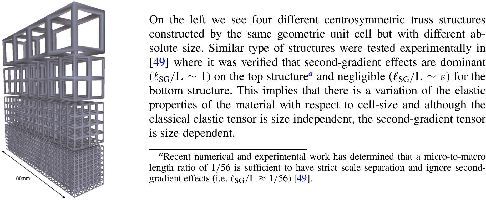
Generalized continuum theories (compare, e.g., [26,28,29,45–48,56,65,66]) have been consistently applied to modelling of materials with microstructure, such as granular or fibrous materials, or materials with a lattice structure (as well as other non-simple material, see, e.g., [44]). Generalized continuum theories are largely split into higher-gradient methods (e.g., second-gradient material [23,45–48,66]) or higher order methods (e.g., Cosserat material [17,27,38–40,57,59]). Both theories are general enough to quantitatively delineate higher-gradients or higher-order models that incorporate chirality and microstructural scale-size effects. Scale-size effects refer to the changes in behavior or characteristics of a structure as its size is altered. Plainly put, it means that things can behave differently or have different properties depending on their size (see Fig. 1). Chiral (or non-centrosymmetric) materials, on the other hand lack a center of symmetry; they are not invariant under inversion of coordinates transformation (see [35]). Chirality may be present at different scales in the material and is a characteristic of engineered materials containing twisted fibres, e.g., wire rope, cables and even biological filaments, e.g., DNA strands (see, e.g., [36]).

Fig. 1.

Scale-size effects highlight that the size or scale of a structure can influence its behavior, strength, as well as other properties. Within the domain of theoretical mechanics, conventional periodic homogenization theories rooted in the Cauchy continuum framework maintain their validity on the condition of pronounced scale separation. However, when the sizes of micro- and macro-structures converge, breaching the realm of comparability, these theories falter and succumb to the manifestation of size effects.

Homogenization methods are particularly well suited for the analysis of heterogeneous materials with periodically distributed microstructures; for technical details, we refer the reader for instance to [5,7,8,12,43,60]. The technique of homogenization has been applied widely to derive effective equations, both of local and non-local nature, in mechanics, physics, chemistry, and in other natural sciences (see, e.g., [10,54,58]) since it can account for the influence of volume fraction, distribution, and morphology. Nevertheless, it is worth noting that the majority of models amenable to homogenization techniques adhere to the classical Cauchy material framework, which regrettably cannot capture scale-size effects due to the inherent size-independence of the classical elastic tensor. Furthermore, the aspect of chirality, a critical characteristic in certain materials, also remains unaddressed by classical Cauchy material. To circumvent this impasse, we propose a solution that entails the application of homogenization methods within an enriched continuum, thereby facilitating the incorporation of scale-size effects and the modeling of chirality. There are two potent ways of enriching the continuum: Allow higher gradients of the displacement field [62,67,68] or allow additional degrees of freedom [30–32]. The current work focuses on the periodic homogenization within the confines of a linear approximation for a second-gradient nonlinear elastic material. The model proposed is sufficiently rich to model chiral-type microstructures and account for scale-size effects by means of dimensional analysis. In doing so, we rigorously derive two different classes of effective models: If the absolute size of the heterogeneities is comparable with the period, then we obtain an effective classical Cauchy continuum. If the absolute size of the heterogeneities is comparable with the overall length of the domain (no scale separation), then we obtain an effective second-gradient material. In the latter case, we recover the boundary conditions and the equilibrium equations for second-gradient theory as originally proposed in [33,47]. Additionally, compared to the classical works in [33,47], we can now compute explicitly the effective coefficients that characterize the material properties, taking into account volume fraction, particle distribution, and morphology. This is a novelty from the methodological point of view. Moreover, since we will be dealing with higher gradients, the choice of method to rigorously pass to the limit plays an important role. Certain techniques of homogenization lend themselves to be more easily exploited in dealing with higher-gradients than others. In this work we will use the method of periodic unfolding [14–16,18] instead of two-scale convergence [4,41,51]. The unfolding method has a natural way of handling higher-gradients without any extra effort, as it was pointed out in the original work [15]. Furthermore, the results presented here can be extended to domains with holes by adjusting the periodic unfolding operator as in [13].

To fix ideas, we designate an origin and the natural orthonormal basis in ${IR}^{3}$ and we choose the reference configuration to coincide with the natural or stress-free configuration. We denote by $\overline{Ω}$ the region occupied in the reference configuration, which is the closure of a domain $Ω \subset {IR}^{3}$ and we call $\overline{Ω}$ the elastic body. We further, assume that the boundary $Σ : = \partial Ω$ is sufficiently smooth. If $ψ (x)$ is the deformation map then the material response of the elastic body is described by a stored energy W that is a real-valued function of the deformation gradient $F : = \nabla ψ$ 1

We have made the standard assumption that $F \in {M \in GL ({IR}^{3}) | \det (M) > 0}$ where $GL ({IR}^{3})$ represents the general linear group of order 3 while the third order tensors will be symmetric in their first two indices. For a more detailed setting the reader can consult [42].

and the gradient of the deformation gradient

G : = \nabla \nabla ψ

. We denote by

\tilde{u} (x) : = ψ (x) - x

the displacement and assume that follows some scaling

\tilde{u} (x) : = α u (x)

, for some positive constant α (we clarify later where we make use of such an α). Elementary calculations yield immediately,

F = I + α \nabla u

, where I is the second order identity tensor.

Notation: To expedite the presentation of our results, here onwards we will make use of the following notation: We will use the Einstein summation for repeated indices unless otherwise stated. Moreover, we will use the symbols : and ⋮ to indicate second order contractions and third order contractions among tensors, respectively, while $ϵ_{i j k}$ will be the Levi-Civita permutation tensor.

The internal energy of the elastic body is given by, $\begin{matrix} (1.1) & E (ψ) = \int_{Ω} W (F, G) d x, \end{matrix}$ where the stored energy satisfies the principle of material objectivity.2

$W (Q F, Q G) = W (F, G)$ for all $Q \in SO (3)$ where $SO (3)$ is the space of all orthogonal matrices in ${IR}^{3}$ with determinant equal to 1, $G$ symmetric in their first two components, and $F \in {M \in GL ({IR}^{3}) | \det (M) > 0)}$ .

The equilibrium equations are derived by computing the first variation of

E (ψ)

and equate it to the virtual work of some body force field

g

acting through an admissible variation [42]. Integration by parts, then, gives,

\begin{matrix} (1.2) & - div (\frac{\partial W (F, G)}{\partial F} - div \frac{\partial W (F, G)}{\partial G}) = g in Ω . \end{matrix}

Upon using the classical chain rule we can rewrite the above equation as follows, $\begin{matrix} (1.3) & \begin{aligned} A (F, G) [\nabla^{(4)} ψ] + S (F, & G) [\nabla^{(3)} ψ] - K (F, G) [\nabla \nabla ψ] + b (\nabla^{(3)} ψ, \nabla \nabla ψ) = g \end{aligned} \end{matrix}$ where $\begin{matrix} (1.4) & \begin{aligned} A (F, G) {[\nabla^{(4)} ψ]}_{i} : = \frac{\partial^{2} W}{\partial G_{p q r} \partial G_{i j k}} \frac{\partial^{4} ψ_{p}}{\partial x_{j} \partial x_{k} \partial x_{q} \partial x_{r}}, \\ S (F, G) {[\nabla^{(3)} ψ]}_{i} : = - \frac{\partial^{2} W}{\partial G_{p q r} \partial F_{i j}} \frac{\partial^{3} ψ_{p}}{\partial x_{j} \partial x_{q} \partial x_{r}} + \frac{\partial^{2} W}{\partial F_{p q} \partial G_{i j k}} \frac{\partial^{3} ψ_{p}}{\partial x_{j} \partial x_{k} \partial x_{q}}, \\ K (F, G) {[\nabla \nabla ψ]}_{i} : = \frac{\partial^{2} W}{\partial F_{p q} \partial F_{i j}} \frac{\partial^{2} ψ_{p}}{\partial x_{j} \partial x_{q}}, \\ b_{i} (\nabla^{(3)} ψ, \nabla \nabla ψ) : = [\frac{\partial}{\partial x_{j}} \frac{\partial^{2} W}{\partial G_{p q r} \partial G_{i j k}}] \frac{\partial^{3} ψ_{p}}{\partial x_{k} \partial x_{q} \partial x_{r}} + [\frac{\partial}{\partial x_{j}} \frac{\partial^{2} W}{\partial F_{p q} \partial G_{i j k}}] \frac{\partial^{2} ψ_{p}}{\partial x_{k} \partial x_{q}} . \end{aligned} \end{matrix}$

Throughout the work we assume that the uniform strong ellipticity condition holds, i.e., there exist positive (generic) constants $c_{1}$ and $c_{2}$ such that: $\begin{matrix} (1.5) & c_{1} | w |^{2} | q |^{4} ⩽ w \otimes q \otimes q ⋮ A (F, G) [w \otimes q \otimes q] ⩽ c_{2} | w |^{2} | q |^{4} \end{matrix}$ for all $w, q \in {IR}^{3} - {0}$ and for all $(F, G)$ with $G$ symmetric in the first two components and $F \in {M \in GL ({IR}^{3}) | \det (M) > 0)}$ . Furthermore, at the reference state we assume that, $\begin{matrix} (1.6) & c_{1} | w |^{2} | q |^{2} ⩽ w \otimes q : K (I, 0) [w \otimes q] ⩽ c_{2} | w |^{2} | q |^{2} \end{matrix}$ for all $w, q \in {IR}^{3} - {0}$ . Additionally, we assume that the tensor $S$ belongs to $L^{\infty} (Ω, {IR}^{3 \times 3 \times 3 \times 3 \times 3})$ .

We linearlize equation (1.2) by carrying out a Taylor expansion of the stored energy W around the reference state3

We have added a detailed derivation of the Taylor expansion in the appendix for the readers convenience.

(F, G) = (I, 0)

and we obtain the following classical linearized equations of second-gradient elasticity,

\begin{array}{c} (1.7) & \begin{aligned} - div τ = g in Ω, \\ τ : = σ - div μ in Ω, \end{aligned} \end{array}

where the quantities σ and μ are related to the deformation and the gradient of the deformation by the following constitutive laws:

\begin{matrix} (1.8) & σ = K : \nabla u + S ⋮ \nabla \nabla u, μ = A ⋮ \nabla \nabla u + S : \nabla u, \end{matrix}

which is a mechanical constitutive law up to

O (α)

in the expansion and where,

\begin{array}{c} (1.9) & \begin{aligned} K & : = \frac{\partial^{2} W}{\partial F \partial F} (I, 0), S : = \frac{\partial^{2} W}{\partial F \partial G} (I, 0), A : = \frac{\partial^{2} W}{\partial G \partial G} (I, 0) . \end{aligned} \end{array}

2. Background and set up of the problem

2.1. Dimensional analysis and scaling

The elastic body $\overline{Ω}$ is assumed to be periodic with period ℓ and with characteristic length L. We define the dimensionless coordinates and displacement, $\begin{matrix} (2.1) & x^{*} = \frac{x}{L}, u^{*} (x^{*}) = \frac{u (x)}{L} . \end{matrix}$

Moreover, we define the following non-dimensional tensors: $\begin{aligned} (2.2) & K K^{*} = K, S S^{*} = S, A A^{*} = A \end{aligned}$ where $\begin{aligned} (2.3) & K : = max_{z \in Y_{ℓ}} | K (z) |, S : = max_{z \in Y_{ℓ}} | S (z) |, A : = max_{z \in Y_{ℓ}} | A (z) |, \end{aligned}$ with $Y_{ℓ} : = {(- ℓ / 2, ℓ / 2]}^{3}$ the periodic cell characterizing the body Ω, while $τ^{*} : = K^{- 1} τ$ will be the non-dimensional hyperstress.

In contemporary discourse regarding second-gradient continua, it has been underscored that the utilization of second-order (perhaps even higher-gradient models) becomes imperative when one tries to articulate continuum frameworks for systems characterized by pronounced heterogeneities in physical attributes across different length scales4

⁴
In second-gradient theory there are additional intrinsic lengths related to the microstructure of the material. We refer the reader to reference [6] for a modern review on the topic. Since we are interested in modelling chiral microstructures (reference [37] addresses the modelling of chirality in elastic materials) we will focus our attention on an additional length scale related to chirality.

or when contact force interactions are characterized not solely by a surface density, but also by a line density along the edges of the contact surface, when they exist (see, e.g., [21] and references therein, [20]).

In the context of this work, where we wish to incorporate intrinsic length scales into the constitutive behavior of the structure, we draw upon the methodologies outlined in the works of [31,52], and [53]. Subsequently, we introduce the following length scales, which are intimately linked to the microstructure of the material: $\begin{matrix} (2.4) & A : = K ℓ_{SG}^{2}, S : = K ℓ_{SG}^{1 / p} ℓ_{chiral}^{1 / p^{'}} where \frac{1}{p} + \frac{1}{p^{'}} = 1, p, p^{'} \in (1, \infty) . \end{matrix}$

The rationale behind the aforementioned scaling is twofold: Firstly, it offers a natural means to establish an explicit dependence of the effective properties of a heterogeneous material on the absolute size of the constituents (see, e.g., [31]). Secondly, the scaling5

⁵

Naturally, many other type of scalings can be considered. We chose to work with the aforementioned scalings because of the reasons we laid out above.

(2.4) ensures coherence by stipulating that chiral effects cannot exist in isolation from second-gradient effects. However, second-gradient effects can manifest independently of chiral effects. The interplay between

ℓ_{SG}

and

ℓ_{chiral}

is related to the well-posedness of the model, specifically, to the coercivity of the involved operators. We address this issue in detail in subsequent sections.

The non-dimensional stress in (1.7) has the following form, $\begin{aligned} τ^{*} : = & K^{*} : \nabla^{*} u^{*} + {(\frac{ℓ_{chiral}}{L})}^{1 / p^{'}} {(\frac{ℓ_{SG}}{L})}^{1 / p} S^{*} ⋮ \nabla^{*} \nabla^{*} u^{*} \\ (2.5) & - di v^{*} ({(\frac{ℓ_{SG}}{L})}^{2} A^{*} ⋮ \nabla^{*} \nabla^{*} u^{*} + {(\frac{ℓ_{chiral}}{L})}^{1 / p^{'}} {(\frac{ℓ_{SG}}{L})}^{1 / p} S^{*} : \nabla^{*} u^{*}), \end{aligned}$ where the material tensors $K^{*} (x^{*}) = {K_{j i k ℓ}^{*} (x *)}_{j, i, k, ℓ = 1}^{3}$ , $S^{*} (x^{*}) = {S_{j i}^{k ℓ m *} (x *)}_{j, i, k, ℓ, m = 1}^{3}$ , and $A^{*} (x^{*}) = {A_{i j k}^{n ℓ m *} (x *)}_{j, i, k, n, ℓ, m = 1}^{3}$ are $Y^{*}$ periodic with, $\begin{matrix} (2.6) & Y^{*} : = \frac{ℓ}{L} Y, Y : = {(- \frac{1}{2}, \frac{1}{2}]}^{3} . \end{matrix}$

Thus, one can generate an ε periodic problem by defining the non-dimensional number ε as the ratio of $ℓ / L$ and let $ε \to 0$ to obtain an effective medium. However, different cases ought to be considered depending on how the intrinsic length scales $ℓ_{chiral}$ and $ℓ_{SG}$ scale with ℓ and L, respectively. Here we consider the cases, $\begin{aligned} (HS 1) & ℓ_{SG} / L \sim ε and ℓ_{chiral} / ℓ \sim ε^{p^{'}} \\ (HS 2) & ℓ_{SG} / L \sim 1 and ℓ_{chiral} / ℓ \sim ε^{p^{'} - 1} . \end{aligned}$

Size effects and scale separation. We chose to work with the above scalings, primarily, because of their physical interpretation. The (HS 1) scaling indicates that the absolute size of the heterogeneities are comparable to the order of the period. The (HS 2) scaling indicates that the absolute size of the heterogeneities are comparable to the characteristic length of the overall domain. Moreover, the chirality scaling has a more general form. However, it cannot be chosen independently of $ℓ_{SG}$ . The reason being, as we will show in the next section, well-posedness of the model. In our case, the chirality length is (at least) one order smaller compared to the length of second-gradient effects.

Naturally, one could consider a different scaling than the one proposed above. We will not address other type of scaling here. Rather we will leave their treatment to future work. Finally, henceforth, we will omit the ∗ notation for the sake of simplicity and expediency of presentation.

2.1.1. Scaling of the stress and hyperstress under HS 1

If $ℓ_{chiral} / ℓ = ε^{p^{'}}$ then $ℓ_{chiral} / L = ε^{p^{'} + 1}$ . Hence, the hyperstress becomes, $\begin{array}{c} (2.7) & \begin{aligned} τ^{ε} = K (\frac{x}{ε}) : \nabla u^{ε} & + ε^{2} S (\frac{x}{ε}) ⋮ \nabla \nabla u^{ε} - div (ε^{2} A (\frac{x}{ε}) ⋮ \nabla \nabla u^{ε} + ε^{2} S (\frac{x}{ε}) : \nabla u^{ε}), \end{aligned} \end{array}$ where $\begin{matrix} (2.8) & σ^{ε} = K (\frac{x}{ε}) : \nabla u^{ε} + ε^{2} S (\frac{x}{ε}) ⋮ \nabla \nabla u^{ε} \end{matrix}$ and $\begin{matrix} (2.9) & μ^{ε} = ε^{2} A (\frac{x}{ε}) ⋮ \nabla \nabla u^{ε} + ε^{2} S (\frac{x}{ε}) : \nabla u^{ε} . \end{matrix}$

2.1.2. Scaling of the stress and hyperstress under HS 2

If $ℓ_{SG} / L = 1$ and $ℓ_{chiral} / ℓ = ε^{p^{'} - 1}$ , then $ℓ_{chiral} / L = ε^{p^{'}}$ . Hence, the hyperstress becomes, $\begin{array}{c} (2.10) & \begin{aligned} τ^{ε} = K (\frac{x}{ε}) : \nabla u^{ε} & + ε S (\frac{x}{ε}) ⋮ \nabla \nabla u^{ε} - div (A (\frac{x}{ε}) ⋮ \nabla \nabla u^{ε} + ε S (\frac{x}{ε}) : \nabla u^{ε}), \end{aligned} \end{array}$ where $\begin{matrix} (2.11) & σ^{ε} = K (\frac{x}{ε}) : \nabla u^{ε} + ε S (\frac{x}{ε}) ⋮ \nabla \nabla u^{ε} \end{matrix}$ and $\begin{matrix} (2.12) & μ^{ε} = A (\frac{x}{ε}) ⋮ \nabla \nabla u^{ε} + ε S (\frac{x}{ε}) : \nabla u^{ε} . \end{matrix}$

3. The microscopic model

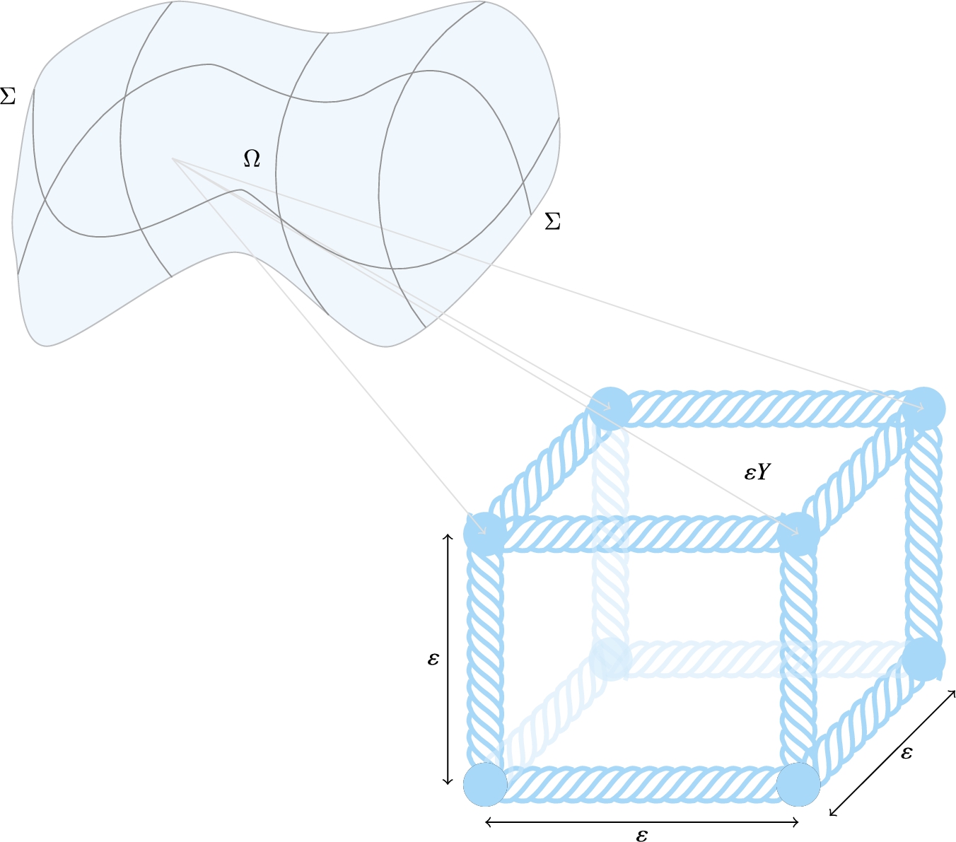
We consider an elastic body with periodic microstructure of period ε occupying a region $Ω \subset {IR}^{3}$ . The region Ω that the body occupies, is assumed to be a uniformly Lipschitz open set (see [22, Definition 2.65]). $Y = {(- 1 / 2, 1 / 2]}^{3}$ is the unit cube in ${IR}^{3}$ , and $Z^{3}$ is the set of all 3–dimensional vectors with integer components. For every positive ε, let $N_{ε}$ be the set of all points $κ \in Z^{3}$ such that $ε (κ + Y)$ is strictly included in Ω. Denote by T be the closure of an open subset in Y with Lipschitz boundary and by $T_{κ}^{ε} : = ε (κ + T)$ will represent the region containing one of the material phases (see Fig. 2).6

⁶
Recent work using topology optimization in [11] has been able to construct chiral microstructures. Although they use a couple stress model which is different than what we propose here, it appears that what we have labeled in this work as $ℓ_{SG}$ and $ℓ_{chiral}$ to be equal to $ℓ_{SG} / L \approx 1$ and $ℓ_{chiral} / L \approx 1$ .

Hence, we can define the following subsets of Ω:

$\begin{matrix} Ω_{1 ε} : = ⋃_{κ \in N_{ε}} T_{κ}^{ε}, Ω_{2 ε} : = Ω ∖ Ω_{1 ε}, Ω : = Ω_{1 ε} \cup Ω_{2 ε} . \end{matrix}$

Fig. 2.

Schematic picture of the domain Ω with a (possible) helical type microstructure. One can imagine the helical microstructure re-enforcing the interior of the unit cell which is filled with a “weak” material where we have assumed perfect interface conditions across the interphase. Second-gradient elasticity allows for the modelling of domains with helical type microstructures, where they respond to compression by twisting.

The exterior boundary component will be denoted by $Σ : = \partial Ω$ . We decompose $Σ : = Σ_{0} \cup Σ_{1}$ with $Σ_{0} \cap Σ_{1} = \emptyset$ a.e. and with both nonempty. The vector $n$ will be the unit normal on Σ, pointing in the outward direction. Moreover, thermodynamic stability bounds require that the tensors $K$ , $A$ , and $S$ possess major symmetries (indicated by the structure of the coefficients in (1.9)). Furthermore, in addition to the conditions imposed by equations (1.5) and (1.6), we assume that $K_{j i k l} \in L^{\infty} (Y)$ , $A_{i j k}^{n ℓ m} \in L^{\infty} (Y)$ , $S_{j i}^{k ℓ m} \in L^{\infty} (Y)$ are bounded, measurable functions that can be extended as Y-periodic functions to the entirety of $R^{3}$ while we reserve the notation for the coefficients, $\begin{matrix} (3.1) & K (\frac{x}{ε}) = K (y), S (\frac{x}{ε}) = S (y), A (\frac{x}{ε}) = A (y) \end{matrix}$ where $y = x / ε$ . In case of isotropy, the above tensors take the following form (see, e.g., [19,63,64]), $\begin{aligned} (3.2) & K_{i j k l} = λ δ_{i j} δ_{k l} + μ (δ_{i k} δ_{j l} + δ_{i l} δ_{j k}), \\ (3.3) & S_{j i}^{k l p} = C_{8} (ϵ_{i k l} δ_{j p} + ϵ_{i k p} δ_{j l} + ϵ_{j k l} δ_{i p} + ϵ_{j k p} δ_{i l}), \\ A_{i j k}^{l p q} = C_{3} (δ_{i j} δ_{k l} δ_{p q} + δ_{i j} δ_{k p} δ_{q l} + δ_{i k} δ_{j q} δ_{l p} + δ_{i q} δ_{j k} δ_{l p}) + C_{4} δ_{i j} δ_{k q} δ_{l p} \\ + C_{5} (δ_{i k} δ_{j l} δ_{p q} + δ_{i k} δ_{j p} δ_{l q} + δ_{i l} δ_{j k} δ_{p q} + δ_{i p} δ_{j k} δ_{l q}) + C_{6} (δ_{i l} δ_{j p} δ_{k q} + δ_{i p} δ_{j l} δ_{k q}) \\ (3.4) & + C_{7} (δ_{i l} δ_{j q} δ_{k p} + δ_{i p} δ_{j q} δ_{k l} + δ_{i q} δ_{j l} δ_{k p} + δ_{i q} δ_{j p} δ_{k l}) . \end{aligned}$

3.1. Auxiliary formulas

For the readers convenience and for the expediency of the our results, we introduce certain formulas that we will make use of in what follows. These formulas can also be found in [33, Appendix].

For any sufficiently smooth scalar function ξ defined on Σ or on a neighborhood of Σ the tangential and normal components of $\nabla ξ$ are, $\begin{matrix} (3.5) & {(\nabla ξ)}_{τ} = - n \times (n \times \nabla ξ) = \nabla ξ - {(\nabla ξ)}_{n} n, {(\nabla ξ)}_{n} : = \nabla ξ \cdot n . \end{matrix}$

Moreover, we introduce the surface gradient of ξ using the projection operator $Π : = I - n \otimes n$ . $\begin{matrix} \nabla_{s} ξ = (I - n \otimes n) \nabla ξ = Π \nabla ξ . \end{matrix}$

Thus, we can write down a useful integration by parts on surfaces formula, $\begin{matrix} (3.6) & \int_{Σ} \nabla_{s} ξ d s = \int_{Σ} ξ (div n) n d s + \int_{\partial Σ} ⟦ ξ ν ⟧ d ℓ, \end{matrix}$ where $ν_{i} = ϵ_{i j k} t_{j} n_{k}$ , $i = 1, 2, 3$ , is a component of the unit normal vector on $\partial Σ$ and tangent to Σ, $t_{j}$ is a component of the unit tangent vector to $\partial Σ$ , and the jump of a vector $f$ across $\partial Σ$ 7

⁷
The bounding surface Σ is a closed surface with piecewise continuous tangent planes and curved surfaces, and we have denoted by $\partial Σ$ the “edges” of Σ, along which a discontinuity of the tangent plane may be observed.

is a function

⟦ f ⟧

\partial Σ

defined by,

\begin{matrix} (3.7) & ⟦ f (x_{0}) ⟧ : = lim_{x \to {x_{0}}^{+}} f (x) - lim_{x \to {x_{0}}^{-}} f (x) with x_{0} \in \partial Σ . \end{matrix}

Lastly, we remark, the jump term on (3.6) is on a ridge, i.e., the line on Σ where the tangent plane of Σ is discontinuous. The above formulas are used with a high degree of frequency in emulsions and capillary fluids (see, e.g., [55]). We refer the reader to the appendix of reference [33,34] for an excellent exposition of the above formulae and related topics.

Using the above formulas and notation, the heterogeneous medium is then be characterized by the following system (written component-wise) for $i = 1, 2, 3$ : $\begin{array}{c} (3.8) & \begin{aligned} - & \partial_{x_{j}} τ_{i j}^{ε} = g_{i} in Ω, \\ τ_{i j}^{ε} = σ_{i j}^{ε} - \partial_{x_{k}} μ_{i j k}^{ε} in Ω, \\ (σ_{i j}^{ε} - \partial_{x_{k}} μ_{i j k}^{ε}) n_{j} - Π_{q ℓ} \partial_{x_{ℓ}} (μ_{i j k}^{ε} n_{k} Π_{q j}) = 0 on Σ_{1}, \\ μ_{i j k}^{ε} n_{k} n_{j} = 0 on Σ_{1}, \\ u_{i}^{ε} = 0 on Σ_{0}, \\ \frac{\partial u_{i}^{ε}}{\partial n} = 0 on Σ_{0}, \\ ⟦ μ_{i j k}^{ε} n_{k} ν_{j} ⟧ = 0 on \partial Σ_{1}, \end{aligned} \end{array}$ where $g_{i}$ is a component some appropriately scaled body force (the scaled body force is $g^{*} = L K^{- 1} g$ )8

⁸

The reader can consult the work in [31, pg. 4589] regarding these type of scalings.

that belongs in

L^{2} (Ω)

and

ν_{i}

is a component of the outward unit normal to

\partial Σ

, for

i = 1, 2, 3

Given that the boundary conditions for a second-gradient material are not as conventional as the boundary conditions for a classical Cauchy material we write out explicitly what mechanical forces they represent on the elastic body following references [33,34]. Thus, besides the classical homogeneous Dirichlet boundary condition, we also have:

Surface traction: $(σ_{i j}^{ε} - \partial_{x_{k}} μ_{i j k}^{ε}) n_{j} - Π_{q ℓ} \partial_{x_{ℓ}} (μ_{i j k}^{ε} n_{k} Π_{q j})$ ,

A normal double traction: $μ_{i j k}^{ε} n_{k} n_{j}$ ,

A line traction: $⟦ μ_{i j k}^{ε} n_{k} ν_{j} ⟧$ .

3.2. Variational formulation

The primary setting for this work is the Sobolev space $H^{2} (Ω, {IR}^{3})$ , the space of functions $u : Ω \mapsto {IR}^{3}$ such that each coordinate is twice weakly differentiable and all the first and second partial derivatives are in $L^{2} (Ω)$ and the subspace $H_{Σ_{0}}^{2} (Ω, {IR}^{3})$ which consists functions that vanish along with their derivatives on the part of the boundary of Σ, $Σ_{0}$ (see, e.g. [1]).

The space $H^{2} (Ω, {IR}^{3})$ is a Hilbert space with norm, $\begin{matrix} (3.9) & ‖ u ‖_{H^{2} (Ω, {IR}^{3})} = {(‖ u ‖_{L^{2} (Ω, {IR}^{3})}^{2} + ‖ \nabla u ‖_{L^{2} (Ω, {IR}^{3 \times 3})}^{2} + ‖ \nabla \nabla u ‖_{L^{2} (Ω, {IR}^{3 \times 3 \times 3})}^{2})}^{1 / 2} . \end{matrix}$

Hence, if we multiply (3.8) by $v \in {C^{\infty} (\overline{Ω}, {IR}^{3}) | v = 0, \nabla v n = 0 on Σ_{0}}$ and integrate by parts, then we obtain: $\begin{matrix} (3.10) & - \int_{Σ_{1}} (σ_{i j}^{ε} - \partial_{x_{k}} μ_{i j k}^{ε}) n_{j} v_{i} d s + \int_{Ω} (σ_{i j}^{ε} - \partial_{x_{k}} μ_{i j k}^{ε}) \partial_{x_{j}} v_{i} d x = \int_{Ω} g_{i} v_{i} d x . \end{matrix}$

A second integration by parts of the second term on the second integral gives, $\begin{aligned} - \int_{Σ_{1}} (σ_{i j}^{ε} - \partial_{x_{k}} μ_{i j k}^{ε}) n_{j} v_{i} d s + \int_{Ω} σ_{i j}^{ε} \partial_{x_{j}} v_{i} d x \\ (3.11) & + \int_{Ω} μ_{i j k}^{ε} \partial_{x_{j} x_{k}}^{2} v_{i} d x - \int_{Σ_{1}} μ_{i j k}^{ε} n_{k} \partial_{x_{j}} v_{i} d s = \int_{Ω} g_{i} v_{i} d x . \end{aligned}$

The last term on the left hand side of the above equation requires a second integration by parts. However, we first decompose it into its normal and tangential component (see equation (3.5)) as follows, $\begin{matrix} (3.12) & \int_{Σ_{1}} μ_{i j k}^{ε} n_{k} \partial_{x_{j}} v_{i} d s = \int_{Σ_{1}} μ_{i j k}^{ε} n_{k} n_{j} n_{l} \partial_{x_{l}} v_{i} d s + \int_{Σ_{1}} μ_{i j k}^{ε} n_{k} Π_{l j} \partial_{x_{l}} v_{i} d s \end{matrix}$

A second integration by parts on surfaces (see equation (3.6)) for the last term on the right hand side of the above equation gives, $\begin{aligned} \int_{Σ_{1}} μ_{i j k}^{ε} n_{k} Π_{l j} \partial_{x_{l}} v_{i} d s & = \int_{Σ_{1}} (μ_{i j k}^{ε} n_{k} Π_{q j} (div n) n_{q} - Π_{q l} \partial_{x_{l}} (μ_{i j k}^{ε} n_{k} Π_{q j})) v_{i} d s \\ (3.13) & - \int_{\partial Σ_{1}} ⟦ μ_{i j k}^{ε} n_{k} ν_{j} v_{i} ⟧ d ℓ . \end{aligned}$

We remark immediately, $\begin{matrix} (3.14) & μ_{i j k}^{ε} n_{k} Π_{q j} (div n) n_{q} = (μ_{i j k}^{ε} n_{k} n_{j} - μ_{i j k}^{ε} n_{k} n_{q} n_{j} n_{q}) (div n) = 0 . \end{matrix}$

Hence, using a density argument, the variational formulation of (3.8) is: Find $u^{ε} \in H_{Σ_{0}}^{2} (Ω, {IR}^{3})$ such that, $\begin{matrix} (3.15) & \int_{Ω} σ_{i j}^{ε} \partial_{x_{j}} v_{i} d x + \int_{Ω} μ_{i j k}^{ε} \partial_{x_{j} x_{k}}^{2} v_{i} d x = \int_{Ω} g_{i} v_{i} d x, \end{matrix}$ for all $v \in H_{Σ_{0}}^{2} (Ω, {IR}^{3})$ .

3.3. Existence and uniqueness

Denote by, $\begin{matrix} (3.16) & B [u^{ε}, v] : = \int_{Ω} σ_{i j}^{ε} \partial_{x_{j}} v_{i} d x + \int_{Ω} μ_{i j k}^{ε} \partial_{x_{j} x_{k}}^{2} v_{i} d x . \end{matrix}$

The form B is evidently a bilinear form that is continuous in the weak topology of $H^{2} \times H^{2}$ and it remains to show coercivity in order to apply the Lax-Milgram theorem.

3.3.1. Coercivity in HS 1

Using the strong ellipticity conditions in (1.5) and (1.6) together with Cauchy’s inequality with δ we obtain, $\begin{aligned} κ_{1} ε^{2} {‖ \nabla \nabla u^{ε} ‖}_{L^{2} (Ω, {IR}^{3 \times 3 \times 3)}}^{2} + c_{1} {‖ \nabla u^{ε} ‖}_{L^{2} (Ω, {IR}^{3 \times 3})}^{2} \\ ⩽ B [u^{ε}, u^{ε}] - 2 ε^{2} \int_{Ω} S_{i j}^{k l m} (\frac{x}{ε}) \frac{\partial^{2} u_{k}^{ε}}{\partial x_{m} \partial x_{l}} \frac{\partial u_{i}^{ε}}{\partial x_{j}} d x \\ ⩽ B [u^{ε}, u^{ε}] + 2 ε^{2} \int_{Ω} | \nabla \nabla u^{ε} | | \nabla u^{ε} | d x \\ (3.17) & ⩽ B [u^{ε}, u^{ε}] + 2 ε^{2} δ {‖ \nabla \nabla u^{ε} ‖}_{L^{2} (Ω, {IR}^{3 \times 3 \times 3})}^{2} + \frac{ε^{2}}{2 δ} {‖ \nabla u^{ε} ‖}_{L^{2} (Ω, {IR}^{3 \times 3})}^{2} . \end{aligned}$

Thus, $\begin{matrix} (3.18) & (κ_{1} - 2 δ) ε^{2} {‖ \nabla \nabla u^{ε} ‖}_{L^{2} (Ω, {IR}^{3 \times 3 \times 3})}^{2} + (c_{1} - \frac{ε^{2}}{2 δ}) {‖ \nabla u^{ε} ‖}_{L^{2} (Ω, {IR}^{3 \times 3})}^{2} ⩽ B [u^{ε}, u^{ε}] . \end{matrix}$

By selecting $δ < κ_{1} / 4$ , using Poincaré’s inequality in $H_{Σ_{0}}^{1} (Ω, {IR}^{3})$ , and then using the smallness of ε to guarantee $(c_{1} - \frac{2 ε^{2}}{κ_{1}}) = : c > 0$ , we ensure the desired ellipticity: $\begin{matrix} (3.19) & min {κ_{1} / 2, c} c_{Ω} ε^{2} {‖ u^{ε} ‖}_{H^{2} (Ω, {IR}^{3})}^{2} ⩽ B [u^{ε}, u^{ε}] . \end{matrix}$

Additionally, starting with (3.18), by utilizing Poincaré’s inequality in $H_{Σ_{0}}^{1} (Ω, {IR}^{3})$ one can obtain the following estimate for the solution (under HS 1): $\begin{matrix} (3.20) & {({‖ u^{ε} ‖}_{H_{Σ_{0}}^{1} (Ω, {IR}^{3})}^{2} + ε^{2} {‖ \nabla \nabla u^{ε} ‖}_{L^{2} (Ω, {IR}^{3 \times 3 \times 3})}^{2})}^{1 / 2} ⩽ const . ‖ g ‖_{L^{2} (Ω, {IR}^{3})}, \end{matrix}$ for some generic constant independent of ε.

3.3.2. Coercivity in HS 2

Coercivity in this case can be shown in exactly the same way as in HS 1. We simply write it down and omit the details, $\begin{matrix} (3.21) & min {κ_{1} / 2, c} c_{Ω} {‖ u^{ε} ‖}_{H^{2} (Ω, {IR}^{3})}^{2} ⩽ B [u^{ε}, u^{ε}] . \end{matrix}$

Naturally, a similar estimate can be obtained under the scheme HS 2, $\begin{matrix} (3.22) & {‖ u^{ε} ‖}_{H^{2} (Ω, {IR}^{3})} ⩽ const . ‖ g ‖_{L^{2} (Ω, {IR}^{3})}, \end{matrix}$ again, the constant is a generic constant independent of ε. Hence, by the Lax-Milgram lemma, under both schemes, there exists a unique solution $u^{ε} \in H_{Σ_{0}}^{2} (Ω, {IR}^{3})$ to (3.15). We also refer the reader to the works of [24,25] regarding coercivity of different generalized continua.

4. Homogenization of the second-gradient continuum

4.1. The periodic unfolding

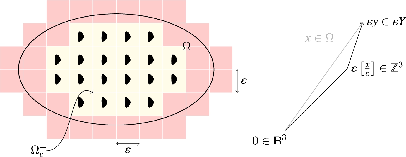
We define the following domain decomposition (see, e.g., [14–16,18]): $\begin{matrix} (4.1) & K_{ε}^{-} : = {ℓ \in Z^{3} | ε (ℓ + Y) \subset \overline{Ω}}, Ω_{ε}^{-} : = int (⋃_{ℓ \in K_{ε}^{-}} ε (ℓ + Y)), Λ_{ε}^{-} : = Ω ∖ Ω_{ε}^{-} . \end{matrix}$

Fig. 3.

Schematic decomposition of the domain and definition of the unfolding operator on a periodic grid.

Let ${[z]}_{Y} = (⌊ z_{1} ⌋, ⌊ z_{2} ⌋, ⌊ z_{3} ⌋)$ denote the integer part of $z \in {IR}^{3}$ and denote by ${z}_{Y}$ the difference $z - {[z]}_{Y}$ which belongs to Y. Regarding our multiscale problem that depends on a small length parameter $ε > 0$ , we can decompose any $x \in {IR}^{3}$ using the maps ${[\cdot]}_{Y} : {IR}^{3} \mapsto Z^{3}$ and ${\cdot}_{Y} : {IR}^{3} \mapsto Y$ the following way (see Fig. 3 (right)), $\begin{matrix} (4.2) & x = ε ({[\frac{x}{ε}]}_{Y} + {\frac{x}{ε}}_{Y}) . \end{matrix}$

For any Lebesgue measurable function φ on Ω we define the periodic unfolding operator by, $\begin{matrix} (4.3) & T_{ε} (φ) (x, y) = \{\begin{array}{ll} φ (ε {[\frac{x}{ε}]}_{Y} + ε y) & for a.e. (x, y) \in Ω_{ε}^{-} \times Y \\ 0 & for a.e. (x, y) \in Λ_{ε}^{-} \times Y . \end{array} \end{matrix}$

Proposition 4.1.

For any $p \in [1, + \infty)$ the unfolding operator $T_{ε} : L^{p} (Ω) \mapsto L^{p} (Ω \times Y)$ is linear, continuous, and has the following properties:

$T_{ε} (φ ψ) = T_{ε} (φ) T_{ε} (ψ)$ for every pair of Lebesgue measurable functions φ, ψ on Ω

For every $φ \in L^{1} (Ω)$ we have, $\begin{matrix} (4.4) & \frac{1}{| Y |} \int_{Ω \times Y} T_{ε} (φ) (x, y) d x d y = \int_{Ω_{ε}^{-}} φ (x) d x = \int_{Ω_{ε}} φ (x) d x - \int_{Λ_{ε}^{-}} φ (x) d x \end{matrix}$

$‖ T_{ε} (φ) ‖_{L^{p} (Ω \times Y)} ⩽ | Y |^{1 / p} ‖ φ ‖_{L^{p} (Ω)}$ for every $φ \in L^{p} (Ω)$

$T_{ε} (φ) \to φ$ strongly in $L^{p} (Ω \times Y)$ for $φ \in L^{p} (Ω)$ as $ε \to 0$

If ${φ_{ε}}_{ε}$ is a sequence in $L^{p} (Ω)$ such that $φ_{ε} \to φ$ strongly in $L^{p} (Ω)$ , then $T_{ε} (φ_{ε}) \to φ$ strongly in $L^{p} (Ω \times Y)$

If $φ \in L^{p} (Y)$ is Y-periodic and $φ_{ε} (x) = φ (\frac{x}{ε})$ then $T_{ε} (φ_{ε}) \to φ$ strongly in $L^{p} (Ω \times Y)$ as $ε \to 0$

If $ϕ_{ε} ⇀ ϕ$ in $H^{1} (Ω)$ then there exists an non-relabelled subsequence and a $\hat{ϕ} \in L^{2} (Ω; H_{per}^{1} (Y))$ such that

$T_{ε} (ϕ_{ε}) ⇀ ϕ$ in $L^{2} (Ω; H^{1} (Y))$

$T_{ε} (\nabla ϕ_{ε}) ⇀ \nabla_{x} ϕ + \nabla_{y} \hat{ϕ}$ in $L^{2} (Ω \times Y, {IR}^{3})$

Let $ϕ_{ε} \in H^{1} (Ω)$ and assume that ${ϕ_{ε}}_{ε}$ is a bounded sequence in $L^{2} (Ω)$ satisfying $ε ‖ \nabla ϕ_{ε} ‖_{L^{2} (Ω; {IR}^{d})} ⩽ c$ (c is a constant independent of ε) then there exists an non-relabelled subsequence and a $\hat{ϕ} \in L^{2} (Ω; H_{per}^{1} (Y))$ such that

$T_{ε} (ϕ_{ε}) ⇀ \hat{ϕ}$ in $L^{2} (Ω; H^{1} (Y))$

$ε T_{ε} (\nabla ϕ_{ε}) ⇀ \nabla_{y} \hat{ϕ}$ in $L^{2} (Ω \times Y)$

If $ϕ_{ε} ⇀ ϕ$ in $H^{2} (Ω)$ then there exists an non-relabelled subsequence and a $\hat{ϕ} \in L^{2} (Ω; H_{per}^{2} (Y))$ such that

$T_{ε} (ϕ_{ε}) ⇀ ϕ$ in $L^{2} (Ω; H^{2} (Y))$

$T_{ε} (\nabla ϕ_{ε}) ⇀ \nabla_{x} ϕ$ in $L^{2} (Ω \times Y, {IR}^{3})$

$T_{ε} (\nabla \nabla ϕ_{ε}) ⇀ \nabla_{x} \nabla_{x} ϕ + \nabla_{y} \nabla_{y} \hat{ϕ}$ in $L^{2} (Ω \times Y, {IR}^{3 \times 3})$

The proof of Proposition 4.1 can be found in reference [15]. We draw the readers attention to property IX. which deals with unfolding higher gradients (and shows the true usefulness of the unfolding method). The proof of property IX. can be found in reference [15, Theorem 3.6, pg. 1603].

4.2. Presentation and discussion of the main results

In this section we present the main results of our work, discuss their significance and consequences, and address how they compare/differ with results in the current literature. Their, respective, proofs are postponed until Section 4.3.

Theorem 4.1.
If $u^{ε} \in H_{Σ_{0}}^{2} (Ω, {IR}^{3})$ is the solution to ( 3.15 ) then, under the HS 1 scheme, there exist $u^{0} \in H_{Σ_{0}}^{1} (Ω; {IR}^{3})$ , $\hat{u} \in L^{2} (Ω; H_{per}^{2} (Y; {IR}^{3}))$ such that, $\begin{aligned} (4.5) & T_{ε} (u^{ε}) ⇀ u^{0} in L^{2} (Ω; H^{2} (Y; {IR}^{3})), \\ (4.6) & T_{ε} (\nabla u^{ε}) ⇀ \nabla_{x} u^{0} + \nabla_{y} \hat{u} in L^{2} (Ω; H^{1} (Y; {IR}^{3 \times 3})), \\ (4.7) & T_{ε} (ε \nabla \nabla u^{ε}) ⇀ \nabla_{y} \nabla_{y} \hat{u} in L^{2} (Ω \times Y; {IR}^{3 \times 3 \times 3}), \end{aligned}$ and $(u^{0}, \hat{u})$ is the unique solution set of, $\begin{aligned} \int_{Ω \times Y} K (y) (\nabla_{x} u^{0} + \nabla_{y} \hat{u}) : (\nabla_{x} V + \nabla_{y} \overline{W}) d y d x \\ (4.8) & + \int_{Ω \times Y} A (y) \nabla_{y} \nabla_{y} \hat{u} ⋮ \nabla_{y} \nabla_{y} \overline{W} d y d x = \int_{Ω \times Y} g \cdot V d y d x, \end{aligned}$ for all $V \in H_{Σ_{0}}^{1} (Ω; {IR}^{3})$ and $\overline{W} \in L^{2} (Ω; H^{2} (Y; {IR}^{3}))$ . Furthermore, ( 4.8 ) is equivalent to the following, $\begin{aligned} (4.9) & \int_{Ω} K^{eff} \nabla_{x} u^{0} : \nabla_{x} V d x = \int_{Ω} g \cdot V d x, \end{aligned}$ if ${\hat{u}}_{i} (x, y) = \frac{\partial u_{α}^{0}}{\partial_{x_{β}}} (x) φ_{i}^{α β} (y) + κ_{i} (x)$ , for $i = 1, 2, 3$ , and we select $\overline{W} \equiv 0$ . Here, $\begin{matrix} (4.10) & K_{i j α β}^{eff} : = \int_{Y} K_{i j k l} (y) (δ_{α k} δ_{β l} + \frac{\partial}{\partial_{y_{l}}} φ_{k}^{α β}) d y, \end{matrix}$ where $φ^{α β}$ is the unique solution (up to a constant) to, $\begin{array}{c} (4.11) & \{\begin{array}{l} - di v_{y} (K : (e_{α} \otimes e_{β} + \nabla_{y} φ^{α β}) - di v_{y} (A ⋮ \nabla_{y} \nabla_{y} φ^{α β})) = 0 in Y, \\ φ^{α β} (y) is Y -periodic . \end{array} \end{array}$

The model in Theorem 4.1 approximates a second-gradient heterogeneous material with chiral effects by a homogeneous classical linear elastic material. Thus, through homogenization we arrive to a non-local constitutive law where the non-locality is a due to the scaling (HS 1). There are two main differences from the models that exist in the literature: First, $u^{ε}$ possesses higher regularity due to Sobolev embedding theory. Indeed, the solution $u^{ε}$ of (3.15) under (HS 1) is (Hölder) continuous $C^{0, λ} (Ω, {IR}^{3})$ , for all $λ \in (0, 1 / 2)$ since, $\begin{matrix} H^{2} (Ω, {IR}^{3}) ↪ C^{0, λ} (\overline{Ω}, {IR}^{3}) \forall λ \in (0, 1 / 2), \end{matrix}$ with the embedding being compact [22, Theorem 2.84, pg. 98]. Second, the structure of the corrector problem in (4.11). The corrector solutions are constructed using second-gradient theory and depend both on the material tensor $K$ as well as the tensor $A$ . Moreover, when no second-gradient effects are present, i.e., the tensor $A$ is identically zero, we recover the classical corrector problem as in references [7,8,12,43,60]. Additionally, the corrector solution inherits the same regularity as $u^{ε}$ and, with it, all the attributes that make it more appealing from the point of view of computational mechanics, i.e., Hölder continuity.
Theorem 4.2.
If $u^{ε} \in H_{Σ_{0}}^{2} (Ω, {IR}^{3})$ is the solution to ( 3.15 ) then, under the HS 2 scheme, there exist $u^{0} \in H_{Σ_{0}}^{2} (Ω, {IR}^{3})$ , $\hat{u} \in L^{2} (Ω; H_{per}^{2} (Y; {IR}^{3}))$ such that, $\begin{aligned} (4.12) & T_{ε} (u^{ε}) ⇀ u^{0} in L^{2} (Ω; H^{2} (Y; {IR}^{3})), \\ (4.13) & T_{ε} (\nabla u^{ε}) ⇀ \nabla_{x} u^{0} in L^{2} (Ω; H^{1} (Y; {IR}^{3 \times 3})), \\ (4.14) & T_{ε} (\nabla \nabla u^{ε}) ⇀ \nabla_{x} \nabla_{x} u^{0} + \nabla_{y} \nabla_{y} \hat{u} in L^{2} (Ω \times Y; {IR}^{3 \times 3 \times 3}), \end{aligned}$ and $(u^{0}, \hat{u})$ is the unique solution set of, $\begin{aligned} \int_{Ω \times Y} K (y) \nabla_{x} u^{0} : \nabla_{x} V d y d x \\ + \int_{Ω \times Y} A (y) (\nabla_{x} \nabla_{x} u^{0} + \nabla_{y} \nabla_{y} \hat{u}) ⋮ (\nabla_{x} \nabla_{x} V + \nabla_{y} \nabla_{y} \overline{W}) d y d x \\ (4.15) & = \int_{Ω \times Y} g \cdot V d y d x, \end{aligned}$ for all $V \in H_{Σ_{0}}^{2} (Ω, {IR}^{3})$ and $\overline{W} \in L^{2} (Ω; H^{2} (Y; {IR}^{3}))$ . Furthermore, ( 4.15 ) is equivalent to the following, $\begin{aligned} (4.16) & \int_{Ω} {⟨ K ⟩}_{Y} \nabla_{x} u^{0} : \nabla_{x} V d x + \int_{Ω} A^{eff} \nabla_{x} \nabla_{x} u^{0} ⋮ \nabla_{x} \nabla_{x} V d x = \int_{Ω} g \cdot V d x, \end{aligned}$ if ${\hat{u}}_{i} (x, y) = \frac{\partial^{2} u_{α}^{0} (x)}{\partial_{x_{β}} \partial_{x_{γ}}} w_{i}^{α β γ} (y) + κ_{i} (x)$ , for $i = 1, 2, 3$ , and we select $\overline{W} \equiv 0$ . Here, $\begin{matrix} (4.17) & {(A^{eff})}_{α β γ}^{i j k} : = \int_{Y} A_{n ℓ m}^{i j k} (y) (δ_{α n} δ_{β m} δ_{γ ℓ} + \frac{\partial^{2}}{\partial_{y_{m}} \partial_{y_{ℓ}}} w_{n}^{α β γ}) d y, \end{matrix}$ where $w^{α β γ}$ is the unique solution (up to an affine displacement in the variable $y$ 9
⁹
In an isotropic medium, it would suffice if one excludes rigid body displacements in the variable $y$ due to the symmetries in the tensor coefficients.

) to, $\begin{array}{c} (4.18) & \{\begin{array}{l} - di v_{y} (di v_{y} (A ⋮ (e_{α} \otimes e_{β} \otimes e_{γ} + \nabla_{y} \nabla_{y} w^{α β γ}))) = 0 in Y, \\ w^{α β γ} (y) is Y -periodic . \end{array} \end{array}$

The results of Theorem 4.2, to our knowledge, are new in their entirety. First, the effective problem (4.16) is of second-gradient type where the effective coefficients are computed using the sixth order tensor $A$ while the fourth order tensor $K$ is simply averaged over the unit cell Y. Moreover, we draw the readers attention to the structure of the corrector problem in (4.18) and how it differs from the corrector problem in (4.11). It is immediate, that problem (4.18) uses three different unit “directional” basis vectors $e_{α}$ , $e_{β}$ , $e_{γ}$ instead of the usual two unit “directional” basis vectors as is standard in the classical theory of elasticity. Furthermore, the same regularity properties, as in the first case, are retained in Theorem 4.2 both for $u^{0}$ and the corrector solution.

Lastly, we remark that the vastly different limit problems obtained under the schemes (HS 1) and (HS 2), respectively, are solely due to the internal lengths, $ℓ_{SG}$ and $ℓ_{chiral}$ , that second-gradient theory introduces. Namely, when the size of the heterogeneities is comparable with the length of the period then we obtain an effective linear elastic material (with higher corrector regularity as a byproduct). When the size of the heterogeneities is comparable with the overall length of the domain (when scale separation is not possible) then the second-gradient effects are retained on the macroscale and the structure of the corrector problem changes considerably. However, the $H^{2}$ regularity of the solution and the corrector is preserved.
4.3. Proofs of the main results

4.3.1. Proof of Theorem 4.1

Theorem 4.1.
If $u^{ε} \in H_{Σ_{0}}^{2} (Ω, {IR}^{3})$ is the solution to ( 3.15 ) then, under the HS 1 scheme, there exist $u^{0} \in H_{Σ_{0}}^{1} (Ω; {IR}^{3})$ , $\hat{u} \in L^{2} (Ω; H_{per}^{2} (Y; {IR}^{3}))$ such that, $\begin{aligned} (4.5) & T_{ε} (u^{ε}) ⇀ u^{0} in L^{2} (Ω; H^{2} (Y; {IR}^{3})), \\ (4.6) & T_{ε} (\nabla u^{ε}) ⇀ \nabla_{x} u^{0} + \nabla_{y} \hat{u} in L^{2} (Ω; H^{1} (Y; {IR}^{3 \times 3})), \\ (4.7) & T_{ε} (ε \nabla \nabla u^{ε}) ⇀ \nabla_{y} \nabla_{y} \hat{u} in L^{2} (Ω \times Y; {IR}^{3 \times 3 \times 3}), \end{aligned}$ and $(u^{0}, \hat{u})$ is the unique solution set of, $\begin{aligned} \int_{Ω \times Y} K (y) (\nabla_{x} u^{0} + \nabla_{y} \hat{u}) : (\nabla_{x} V + \nabla_{y} \overline{W}) d y d x \\ (4.8) & + \int_{Ω \times Y} A (y) \nabla_{y} \nabla_{y} \hat{u} ⋮ \nabla_{y} \nabla_{y} \overline{W} d y d x = \int_{Ω \times Y} g \cdot V d y d x, \end{aligned}$ for all $V \in H_{Σ_{0}}^{1} (Ω; {IR}^{3})$ and $\overline{W} \in L^{2} (Ω; H^{2} (Y; {IR}^{3}))$ . Furthermore, ( 4.8 ) is equivalent to the following, $\begin{aligned} (4.9) & \int_{Ω} K^{eff} \nabla_{x} u^{0} : \nabla_{x} V d x = \int_{Ω} g \dots V d x, \end{aligned}$ if ${\hat{u}}_{i} (x, y) = \frac{\partial u_{α}^{0}}{\partial_{x_{β}}} (x) φ_{i}^{α β} (y) + κ_{i} (x)$ , for $i = 1, 2, 3$ , and we select $\overline{W} \equiv 0$ . Here, $\begin{matrix} (4.10) & K_{i j α β}^{eff} : = \int_{Y} K_{i j k l} (y) (δ_{α k} δ_{β l} + \frac{\partial}{\partial_{y_{l}}} φ_{k}^{α β}) d y, \end{matrix}$ where $φ^{α β}$ is the unique solution (up to a constant) to, $\begin{array}{c} (4.11) & \{\begin{array}{l} - di v_{y} (K : (e_{α} \otimes e_{β} + \nabla_{y} φ^{α β}) - di v_{y} (A ⋮ \nabla_{y} \nabla_{y} φ^{α β})) = 0 in Y, \\ φ^{α β} (y) is Y -periodic . \end{array} \end{array}$
Proof.
Using (3.20) and Proposition 4.1 $V I I$ . we obtain (4.5)–(4.6). To obtain (4.7) apply Proposition 4.1 $I X$ . with $ϕ_{ε} = \nabla u^{ε}$ and the result follows.

We now proceed by unfolding (3.15), under the HS 1 scheme, and apply Proposition 4.1 properties I., II., and VI., to obtain, $\begin{aligned} \int_{Ω \times Y} (K_{i j k l} (y) T_{ε} (\frac{\partial u_{k}^{ε}}{\partial x_{l}}) T_{ε} (\frac{\partial v_{i}}{\partial x_{j}}) + ε^{2} S_{i j}^{k l m} (y) T_{ε} (\frac{\partial^{2} u_{k}^{ε}}{\partial x_{m} \partial x_{l}}) T_{ε} (\frac{\partial v_{i}}{\partial x_{j}})) d y d x \\ + \int_{Ω \times Y} (ε^{2} A_{n l m}^{i j k} (y) T_{ε} (\frac{\partial^{2} u_{n}^{ε}}{\partial x_{l} \partial x_{m}}) T_{ε} (\frac{\partial^{2} v_{i}}{\partial x_{j} \partial x_{k}}) \\ (4.19) & + ε^{2} S_{n l}^{i j k} (y) T_{ε} (\frac{\partial u_{n}^{ε}}{\partial x_{l}}) T_{ε} (\frac{\partial^{2} v_{i}}{\partial x_{j} \partial x_{k}})) d y d x = \int_{Ω \times Y} T_{ε} (g_{i}) T_{ε} (v_{i}) d y d x . \end{aligned}$

Set $v : = V (x)$ to be any test function $V \in C_{0}^{\infty} (Ω; {IR}^{3})$ in (4.19). Taking the limit as $ε \to 0$ and using the properties of the unfolding operator (4.5)–(4.7) we obtain, $\begin{array}{c} (4.20) & \begin{array}{r} \int_{Ω \times Y} K (y) (\nabla_{x} u^{0} + \nabla_{y} \hat{u}) : \nabla_{x} V d y d x = \int_{Ω \times Y} g \cdot V d y d x . \end{array} \end{array}$

Select now test functions of the form $v = v^{ε} : = ε U (x) W (\frac{x}{ε})$ where $U \in C_{0}^{\infty} (Ω)$ and $W \in H_{per}^{2} (Y, {IR}^{3})$ . It is clear that $v^{ε} \to 0$ in $L^{2} (Ω, {IR}^{3})$ . Moreover, we have, $\begin{aligned} (4.21) & \frac{\partial v_{i}^{ε}}{\partial x_{j}} = ε \frac{\partial U}{\partial x_{j}} (x) W_{i} (\frac{x}{ε}) + U (x) \frac{\partial W_{i}}{\partial y_{j}} (\frac{x}{ε}), \\ \frac{\partial^{2} v_{i}^{ε}}{\partial x_{j} \partial x_{k}} = ε \frac{\partial^{2} U}{\partial x_{j} \partial x_{k}} (x) W_{i} (\frac{x}{ε}) + \frac{\partial U}{\partial x_{j}} (x) \frac{\partial W_{i}}{\partial y_{k}} (\frac{x}{ε}) \\ (4.22) & + \frac{\partial U}{\partial x_{k}} (x) \frac{\partial W_{i}}{\partial y_{j}} (\frac{x}{ε}) + \frac{1}{ε} U (x) \frac{\partial^{2} W_{i}}{\partial y_{j} \partial y_{k}} (\frac{x}{ε}) . \end{aligned}$

Thus, as $ε \to 0$ , we have $T_{ε} (v_{i}^{ε}) \to 0$ in $L^{2} (Ω \times Y) T_{ε} (\partial_{x_{j}} v_{i}^{ε}) ⇀ \nabla_{y} {\overline{W}}_{i} (x, y)$ in $L^{2} (Ω \times Y)$ , and $T_{ε} (ε \partial_{x_{j} x_{k}}^{2} v_{i}^{ε}) ⇀ \partial_{y_{j} y_{k}}^{2} {\overline{W}}_{i} (x, y)$ in $L^{2} (Ω \times Y)$ where ${\overline{W}}_{i} (x, y) : = U (x) W_{i} (y)$ . Hence, if in the unfolded expression (4.19) use the above test function we obtain, $\begin{aligned} \int_{Ω \times Y} K (y) (\nabla_{x} u^{0} + \nabla_{y} \hat{u}) : \nabla_{y} \overline{W} d y d x \\ (4.23) & + \int_{Ω \times Y} A (y) \nabla_{y} \nabla_{y} \hat{u} ⋮ \nabla_{y} \nabla_{y} \overline{W} d y d x = 0 . \end{aligned}$

Thus, adding (4.20) and (4.23) we obtain, $\begin{aligned} \int_{Ω \times Y} K (y) (\nabla_{x} u^{0} + \nabla_{y} \hat{u}) : (\nabla_{x} V + \nabla_{y} \overline{W}) d y d x \\ (4.24) & + \int_{Ω \times Y} A (y) \nabla_{y} \nabla_{y} \hat{u} ⋮ \nabla_{y} \nabla_{y} \overline{W} d y d x = \int_{Ω \times Y} g \cdot V d y d x . \end{aligned}$

By the density of $C_{0}^{\infty} (Ω) \otimes H_{per}^{2} (Y; {IR}^{3})$ in $L^{2} (Ω; H_{per}^{2} (Y; {IR}^{3}))$ the result holds for all $\overline{W} (x, y) \in L^{2} (Ω; H_{per}^{2} (Y; {IR}^{3}))$ .

If in (4.24) select $V = 0$ , then we can see that $\hat{u}$ depends linearly on $\nabla_{x} u^{0}$ . Hence, the form of $\hat{u}$ looks as follows: $\begin{matrix} (4.25) & {\hat{u}}_{i} (x, y) = \frac{\partial u_{α}^{0}}{\partial_{x_{β}}} (x) φ_{i}^{α β} (y) + κ_{i} (x), \end{matrix}$ where the corrector $φ^{α β}$ is the local solution satisfying the next boundary-value problem, $\begin{array}{c} (4.26) & \{\begin{array}{l} - di v_{y} (K : (e_{α} \otimes e_{β} + \nabla_{y} φ^{α β}) - di v_{y} (A ⋮ \nabla_{y} \nabla_{y} φ^{α β})) = 0 in Y, \\ φ^{α β} (y) is Y -periodic, \end{array} \end{array}$ where the compatibility condition is automatically satisfied due to the periodicity of the problem. Equivalently, we can formulate (4.26) in its weak form: Find $φ^{α β} \in H_{per}^{2} (Y, {IR}^{3})$ such that $\begin{matrix} (4.27) & \int_{Y} (K e_{α} \otimes e_{β} : \nabla_{y} ϕ + K \nabla_{y} φ^{α β} : \nabla_{y} ϕ + A \nabla_{y} \nabla_{y} φ^{α β} ⋮ \nabla_{y} \nabla_{y} ϕ) d y = 0 \end{matrix}$ for all $ϕ \in H_{per}^{2} (Y, {IR}^{3})$ . The existence and uniqueness (up to a constant) of a weak solution to (4.27) follows from the Lax-Milgram Lemma over the space $H_{per}^{2} (Y, {IR}^{3})$ .

Returning to (4.24) and substituting $\overline{W} = 0$ and $\hat{u}$ from (4.25) we obtain, $\begin{aligned} (4.28) & \int_{Ω} K^{eff} \nabla_{x} u^{0} : \nabla_{x} V d x = \int_{Ω} g \dots V d x, \end{aligned}$ where, $\begin{matrix} (4.29) & K_{i j α β}^{eff} : = \int_{Y} K_{i j k l} (y) (δ_{α k} δ_{β l} + \frac{\partial}{\partial_{y_{l}}} φ_{k}^{α β}) d y . \end{matrix}$

If we define $σ^{eff} : = K^{eff} : \nabla_{x} u^{0}$ then $σ^{eff} = {(σ^{eff})}^{⊤}$ is precisely the Cauchy stress in the theory of classical linear elasticity. This completes the proof. □
4.3.2. Proof of Theorem 4.2

Theorem 4.2.
If $u^{ε} \in H_{Σ_{0}}^{2} (Ω, {IR}^{3})$ is the solution to ( 3.15 ) then, under the HS 2 scheme, there exist $u^{0} \in H_{Σ_{0}}^{2} (Ω, {IR}^{3})$ , $\hat{u} \in L^{2} (Ω; H_{per}^{2} (Y; {IR}^{3}))$ such that, $\begin{aligned} (4.12) & T_{ε} (u^{ε}) ⇀ u^{0} in L^{2} (Ω; H^{2} (Y; {IR}^{3})), \\ (4.13) & T_{ε} (\nabla u^{ε}) ⇀ \nabla_{x} u^{0} in L^{2} (Ω; H^{1} (Y; {IR}^{3 \times 3})), \\ (4.14) & T_{ε} (\nabla \nabla u^{ε}) ⇀ \nabla_{x} \nabla_{x} u^{0} + \nabla_{y} \nabla_{y} \hat{u} in L^{2} (Ω \times Y; {IR}^{3 \times 3 \times 3}), \end{aligned}$ and $(u^{0}, \hat{u})$ is the unique solution set of, $\begin{aligned} \int_{Ω \times Y} K (y) \nabla_{x} u^{0} : \nabla_{x} V d y d x \\ + \int_{Ω \times Y} A (y) (\nabla_{x} \nabla_{x} u^{0} + \nabla_{y} \nabla_{y} \hat{u}) ⋮ (\nabla_{x} \nabla_{x} V + \nabla_{y} \nabla_{y} \overline{W}) d y d x \\ (4.15) & = \int_{Ω \times Y} g \dots V d y d x, \end{aligned}$ for all $V \in H_{Σ_{0}}^{2} (Ω, {IR}^{3})$ and $\overline{W} \in L^{2} (Ω; H^{2} (Y; {IR}^{3}))$ . Furthermore, ( 4.15 ) is equivalent to the following, $\begin{aligned} (4.16) & \int_{Ω} {⟨ K ⟩}_{Y} \nabla_{x} u^{0} : \nabla_{x} V d x + \int_{Ω} A^{eff} \nabla_{x} \nabla_{x} u^{0} ⋮ \nabla_{x} \nabla_{x} V d x = \int_{Ω} g \dots V d x, \end{aligned}$ if ${\hat{u}}_{i} (x, y) = \frac{\partial^{2} u_{α}^{0} (x)}{\partial_{x_{β}} \partial_{x_{γ}}} w_{i}^{α β γ} (y) + κ_{i} (x)$ , for $i = 1, 2, 3$ , and we select $\overline{W} \equiv 0$ . Here, $\begin{matrix} (4.17) & {(A^{eff})}_{α β γ}^{i j k} : = \int_{Y} A_{n ℓ m}^{i j k} (y) (δ_{α n} δ_{β m} δ_{γ ℓ} + \frac{\partial^{2}}{\partial_{y_{m}} \partial_{y_{ℓ}}} w_{n}^{α β γ}) d y, \end{matrix}$ where $w^{α β γ}$ is the unique solution (up to an affine displacement in the variable $y$ 10
¹⁰
In an isotropic medium, it would suffice if one excludes rigid body displacements in the variable $y$ due to the symmetries in the tensor coefficients.

) to, $\begin{array}{c} (4.18) & \{\begin{array}{l} - di v_{y} (di v_{y} (A ⋮ (e_{α} \otimes e_{β} \otimes e_{γ} + \nabla_{y} \nabla_{y} w^{α β γ}))) = 0 in Y, \\ w^{α β γ} (y) is Y -periodic . \end{array} \end{array}$
Proof.
Using (3.22) and Proposition 4.1 $I X$ . we obtain (up to a subsequence) the convergences stated in (4.12)–(4.14). We now proceed by unfolding (3.15), under the HS 2 scheme. To this end, we apply Proposition 4.1 properties I., II., and VI., to obtain $\begin{aligned} \int_{Ω \times Y} (K_{i j k l} (y) T_{ε} (\frac{\partial u_{k}^{ε}}{\partial x_{l}}) T_{ε} (\frac{\partial v_{i}}{\partial x_{j}}) + ε S_{i j}^{k l m} (y) T_{ε} (\frac{\partial^{2} u_{k}^{ε}}{\partial x_{m} \partial x_{l}}) T_{ε} (\frac{\partial v_{i}}{\partial x_{j}})) d y d x \\ + \int_{Ω \times Y} (A_{n l p}^{i j k} (y) T_{ε} (\frac{\partial^{2} u_{n}^{ε}}{\partial x_{l} \partial x_{p}}) T_{ε} (\frac{\partial^{2} v_{i}}{\partial x_{j} \partial x_{k}}) + ε S_{n l}^{i j k} (y) T_{ε} (\frac{\partial u_{n}^{ε}}{\partial x_{l}}) T_{ε} (\frac{\partial^{2} v_{i}}{\partial x_{j} \partial x_{k}})) d y d x \\ (4.30) & = \int_{Ω \times Y} T_{ε} (g_{i}) T_{ε} (v_{i}) d y d x . \end{aligned}$

Set $v : = V (x)$ to be any test function $V \in C_{0}^{\infty} (Ω; {IR}^{3})$ in (4.30). Taking the limit as $ε \to 0$ and using the properties of the unfolding operator (4.12)–(4.14) we obtain, $\begin{aligned} \int_{Ω \times Y} K (y) \nabla_{x} u^{0} : \nabla_{x} V d y d x \\ + \int_{Ω \times Y} A (y) (\nabla_{x} \nabla_{x} u^{0} + \nabla_{y} \nabla_{y} \hat{u}) ⋮ \nabla_{x} \nabla_{x} V d y d x \\ (4.31) & = \int_{Ω \times Y} g \dots V d x . \end{aligned}$

Select now test functions of the form $v = v^{ε} : = ε^{2} U (x) W (\frac{x}{ε})$ where $U \in C_{0}^{\infty} (Ω)$ and $W \in H_{per}^{2} (Y, {IR}^{3})$ . We note that $v^{ε} \to 0$ in $L^{2} (Ω, {IR}^{3})$ . Moreover, we have $\begin{matrix} (4.32) & \frac{\partial v_{i}^{ε}}{\partial x_{j}} = ε^{2} \frac{\partial U}{\partial x_{j}} (x) W_{i} (\frac{x}{ε}) + ε U (x) \frac{\partial W_{i}}{\partial y_{j}} (\frac{x}{ε}), \end{matrix}$ $\begin{aligned} \frac{\partial^{2} v_{i}^{ε}}{\partial x_{j} \partial x_{k}} & = ε^{2} \frac{\partial^{2} U}{\partial x_{j} \partial x_{k}} (x) W_{i} (\frac{x}{ε}) + ε \frac{\partial U}{\partial x_{j}} (x) \frac{\partial W_{i}}{\partial y_{k}} (\frac{x}{ε}) \\ (4.33) & + ε \frac{\partial U}{\partial x_{k}} (x) \frac{\partial W_{i}}{\partial y_{j}} (\frac{x}{ε}) + U (x) \frac{\partial^{2} W_{i}}{\partial y_{j} \partial y_{k}} (\frac{x}{ε}) . \end{aligned}$

Thus, as $ε \to 0$ , it yields $T_{ε} (\partial_{x_{j}} v_{i}^{ε}) \to 0$ in $L^{2} (Ω \times Y)$ and $T_{ε} (\partial_{x_{j} x_{k}}^{2} v_{i}^{ε}) \to \partial_{y_{j} y_{k}}^{2} {\overline{W}}_{i} (x, y)$ in $L^{2} (Ω \times Y)$ for ${\overline{W}}_{i} (x, y) : = U (x) W_{i} (y)$ . Hence, we use the above test functions in the unfolded expression (4.30) to obtain, $\begin{array}{c} (4.34) & \begin{array}{r} \int_{Ω \times Y} A (y) (\nabla_{x} \nabla_{x} u^{0} + \nabla_{y} \nabla_{y} \hat{u}) ⋮ \nabla_{y} \nabla_{y} \overline{W} d y d x = 0 . \end{array} \end{array}$

Adding (4.31) and (4.34), we obtain, $\begin{aligned} \int_{Ω \times Y} K (y) \nabla_{x} u^{0} : \nabla_{x} V d y d x \\ + \int_{Ω \times Y} A (y) (\nabla_{x} \nabla_{x} u^{0} + \nabla_{y} \nabla_{y} \hat{u}) ⋮ (\nabla_{x} \nabla_{x} V + \nabla_{y} \nabla_{y} \overline{W}) d y d x \\ (4.35) & = \int_{Ω} g \dots V d x . \end{aligned}$

Once again, by the density of $C_{0}^{\infty} (Ω) \otimes H_{per}^{2} (Y; {IR}^{3})$ in $L^{2} (Ω; H_{per}^{2} (Y; {IR}^{3}))$ the result holds for all $\overline{W} (x, y) \in L^{2} (Ω; H_{per}^{2} (Y; {IR}^{3}))$ .

Proceeding in a similar fashion as for the case HS 1, if we select in (4.35) $V = 0$ , then we can see that $\hat{u}$ depends linearly on $\nabla_{x} \nabla_{x} u^{0}$ . Hence, the structure of $\hat{u}$ looks as follows, $\begin{matrix} (4.36) & {\hat{u}}_{i} (x, y) = \frac{\partial^{2} u_{α}^{0}}{\partial_{x_{β}} \partial_{x_{γ}}} (x) w_{i}^{α β γ} (y) + P_{i} (x), \end{matrix}$ where $P_{i} (x)$ is a linear polynomial in the variable y and the corrector $w^{α β γ}$ is the local solution satisfying the following problem, $\begin{array}{c} (4.37) & \{\begin{array}{l} - di v_{y} (di v_{y} (A ⋮ (e_{α} \otimes e_{β} \otimes e_{γ} + \nabla_{y} \nabla_{y} w^{α β γ}))) = 0 in Y, \\ w^{α β γ} (y) is Y -periodic . \end{array} \end{array}$

Equivalently, we can formulate (4.37) in its weak form: Find $w^{α β γ} \in H_{per}^{2} (Y, {IR}^{3})$ such that, $\begin{array}{c} (4.38) & \begin{array}{r} \int_{Y} (A e_{α} \otimes e_{β} \otimes e_{γ} ⋮ \nabla_{y} \nabla_{y} ξ + A \nabla_{y} \nabla_{y} w^{α β γ} ⋮ \nabla_{y} \nabla_{y} ξ) d y = 0 . \end{array} \end{array}$

The existence and uniqueness (up to an affine displacement in the $y$ variable) of a weak solution follows based on the Lax-Milgram Lemma. This is straightforward as the Poincaré’s inequality holds for the quotient space $H^{2} (Y) / P$ , where we designate $P$ to be the space of linear polynomials (see, e.g. [50]).

We return now to (4.35). Substituting $\overline{W} = 0$ and $\hat{u}$ from (4.36) we obtain, $\begin{aligned} (4.39) & \int_{Ω} {⟨ K ⟩}_{Y} \nabla_{x} u^{0} : \nabla_{x} V d x + \int_{Ω} A^{eff} \nabla_{x} \nabla_{x} u^{0} ⋮ \nabla_{x} \nabla_{x} V d x = \int_{Ω} g \dots V d x, \end{aligned}$ where, $\begin{array}{c} (4.40) & {⟨ K ⟩}_{Y} : = \int_{Y} K (y) d y, \\ (4.41) & {(A^{eff})}_{α β γ}^{i j k} : = \int_{Y} A_{n ℓ p}^{i j k} (y) (δ_{α n} δ_{β p} δ_{γ ℓ} + \frac{\partial^{2}}{\partial_{y_{p}} \partial_{y_{ℓ}}} w_{n}^{α β γ}) d y . \end{array}$

This completes the proof. □
Remark 4.1.
The coefficient $A^{eff}$ is precisely the coefficient provided phenomenologically by references [33,47], however, in our case it is exactly computable based on volume fraction and morphology of the microstructure.
4.3.3. Recovery of an effective second-gradient theory

The statement of Theorem 4.2 points out a key aspect – we are dealing macroscopically with a second-gradient material (see (4.16)). In this section, we derive the associated partial differential equations with its boundary conditions in the sense of distributions and show that they form a complete set of equilibrium equations for the second-gradient theory of [47] equivalent to the system given by [33].

We begin with, $\begin{aligned} (4.42) & \int_{Ω} {⟨ K ⟩}_{Y} \nabla_{x} u^{0} : \nabla_{x} V d x + \int_{Ω} A^{eff} \nabla_{x} \nabla_{x} u^{0} ⋮ \nabla_{x} \nabla_{x} V d x = \int_{Ω} g \dots V d x \end{aligned}$ and set $\begin{matrix} (4.43) & σ_{p q}^{eff} : = ⟨ K_{p q i j} ⟩ \frac{\partial u_{i}^{0}}{\partial x_{j}}, μ_{p q r}^{eff} : = {(A^{eff})}_{i j k}^{p q r} \frac{\partial^{2} u_{i}^{0}}{\partial x_{j} \partial x_{k}} . \end{matrix}$

Then (4.42) becomes, $\begin{aligned} (4.44) & \int_{Ω} σ_{p q}^{eff} \frac{\partial V_{p}}{\partial x_{q}} d x + \int_{Ω} μ_{p q r}^{eff} \frac{\partial^{2} V_{p}}{\partial x_{r} \partial x_{q}} d x = \int_{Ω} g_{p} V_{p} d x . \end{aligned}$

Integrating by parts the first term once and the second term twice, we obtain, $\begin{aligned} \int_{Σ} (σ_{p q}^{eff} - \partial_{x_{r}} μ_{p q r}^{eff}) n_{q} V_{p} d s - \int_{Ω} \partial_{x_{q}} (σ_{p q}^{eff} - \partial_{x_{r}} μ_{p q r}^{eff}) V_{p} d x \\ (4.45) & + \int_{Σ} μ_{p q r}^{eff} n_{r} \partial_{x_{q}} V_{p} d s = \int_{Ω} g_{p} V_{p} d x . \end{aligned}$

As before, we decompose the boundary term into normal and tangential components via, $\begin{matrix} (4.46) & \int_{Σ} μ_{p q r}^{eff} n_{r} \partial_{x_{q}} V_{p} d s = \int_{Σ} μ_{p q r}^{eff} n_{q} n_{r} n_{l} \partial_{x_{l}} V_{p} d s + \int_{Σ} μ_{p q r}^{eff} n_{r} Π_{l q} \partial_{x_{l}} V_{p} d s . \end{matrix}$

The first component of the above formula is a normal double traction while the second term we integrate by parts (on the surface Σ) using (3.6) and obtain, $\begin{matrix} (4.47) & \int_{Σ} μ_{p q r}^{eff} n_{r} Π_{l q} \partial_{x_{l}} V_{p} d s = - \int_{Σ} Π_{m l} \partial_{x_{l}} (μ_{p q r}^{eff} n_{r} Π_{m q}) V_{p} d s + \int_{\partial Σ} ⟦ μ_{p q r}^{eff} n_{r} ν_{p} ⟧ V_{p} d ℓ . \end{matrix}$

Thus, putting everything together, we have that (4.42) is equivalent to the following identity: $\begin{aligned} \int_{Σ} ((σ_{p q}^{eff} - \partial_{x_{r}} μ_{p q r}^{eff}) n_{q} - Π_{m l} \partial_{x_{l}} (μ_{p q r}^{eff} n_{r} Π_{m q})) V_{p} d s - \int_{Ω} \partial_{x_{q}} (σ_{p q}^{eff} - \partial_{x_{r}} μ_{p q r}^{eff}) V_{p} d x \\ (4.48) & + \int_{Σ} μ_{p q r}^{eff} n_{q} n_{r} n_{l} \partial_{x_{l}} V_{p} d s + \int_{\partial Σ} ⟦ μ_{p q r}^{eff} n_{r} ν_{p} ⟧ V_{p} d ℓ = \int_{Ω} g_{p} V_{p} d x . \end{aligned}$

From the above equation, we can recover the following boundary conditions on Σ and $\partial Σ$ ,

surface traction: $(σ_{p q}^{eff} - \partial_{x_{r}} μ_{p q r}^{eff}) n_{q} - Π_{m l} \partial_{x_{l}} (μ_{p q r}^{eff} n_{r} Π_{m q}) = 0$ on $Σ_{1}$ ,

a normal double traction: $μ_{p q r}^{eff} n_{q} n_{r} = 0$ on $Σ_{1}$ ,

a line traction: $⟦ μ_{p q r}^{eff} n_{r} ν_{p} ⟧ = 0$ on $\partial Σ_{1}$ ,

$u^{0} = 0$ and $\nabla u^{0} n = 0$ on $Σ_{0}$ (the boundary conditions are a-priori in the function space),

which, jointly with the field equations,

\begin{matrix} (4.49) & - \partial_{x_{q}} (σ_{p q}^{eff} - \partial_{x_{r}} μ_{p q r}^{eff}) = g_{p} in D^{'} (Ω), \end{matrix}

build the complete set of equations governing equilibrium states for the second-gradient theory of reference [33,47].

Footnotes

Acknowledgements

The authors gratefully acknowledge the financial support by the Knowledge Foundation (project nr. KK 2020-0152). Moreover, we would like to express our sincere gratitude to the anonymous reviewers for their many comments, suggestions, and corrections. Their comments have, without a doubt, improved the quality of the manuscript. Furthermore, G.N. would like to extends his appreciation to Prof. Dr. Michael Stingl (FAU Erlangen–Nürnmberg) and his Continuous Optimization group for their hospitality where part of this work was completed.

Taylor expansion of the stored energy function around the equilibrium

We perform a Taylor expansion of the stored energy function around the equilibrium. In principle we can continue this expansion and obtain any desired degree of accuracy of the nonlinear energy W. However, using the scaling introduce previously, we keep only the terms up to $O (α^{3})$ leading to, $\begin{aligned} W (x, F, G,) & = W (x, I, 0) + \frac{\partial W}{\partial F_{i j}} (x, I, 0) (F_{i j} - δ_{i j}) + \frac{\partial W}{\partial G_{i j k}} (x, I, 0) \partial_{x_{k}} F_{i j} \\ + \frac{1}{2} \frac{\partial^{2} W}{\partial F_{i j} \partial F_{k ℓ}} (x, I, 0) (F_{i j} - δ_{i j}) (F_{k ℓ} - δ_{k ℓ}) \\ + \frac{\partial^{2} W}{\partial F_{i j} \partial G_{k ℓ m}} (x, I, 0) (F_{i j} - δ_{i j}) \partial_{x_{m}} F_{k ℓ} \\ + \frac{1}{2} \frac{\partial^{2} W}{\partial G_{i j k} \partial G_{m ℓ p}} (x, I, 0) \partial_{x_{k}} F_{i j} \partial_{x_{p}} F_{m ℓ} + O (α^{3}) . \end{aligned}$

The potential energy at the equilibrium configuration is zero and, moreover, we assume that the material is stress free at the equilibrium configuration. Hence, the above expansion reduces to the following, $\begin{aligned} W (x, F, G) & = \frac{1}{2} \frac{\partial^{2} W}{\partial F_{i j} \partial F_{k ℓ}} (x, I, 0) (F_{i j} - δ_{i j}) (F_{k ℓ} - δ_{k ℓ}) \\ + \frac{\partial^{2} W}{\partial F_{i j} \partial G_{k ℓ m}} (x, I, 0) (F_{i j} - δ_{i j}) \partial_{x_{m}} F_{k ℓ} \\ + \frac{1}{2} \frac{\partial^{2} W}{\partial G_{i j k} \partial G_{m ℓ p}} (x, I, 0) \partial_{x_{k}} F_{i j} \partial_{x_{p}} F_{m ℓ} + O (α^{3}) . \end{aligned}$

References

R.A.

Adams and

J.F.

Fournier, Sobolev Spaces, Elsevier, 2003.

Agnelli,

Constantinescu and

Nika, Design and testing of 3D-printed microarchitectured polymer materials exhibiting a negative Poisson’s ratio, Cont. Mechanics & Thermodyn. 32(2) (2020), 433–449. doi:10.1007/s00161-019-00851-6.

Agnelli,

Nika and

Constantinescu, Design of thin micro-architectured panels with extension–bending coupling effects using topology optimization, Comput. Methods Appl. Mech. Engrg. 391 (2022), 114496. doi:10.1016/j.cma.2021.114496.

Allaire, Homogenization and two-scale convergence, SIAM J. Math. Anal. 23(6) (1992), 1482–1518. doi:10.1137/0523084.

Allaire, Shape Optimization by the Homogenization Methods, Springer-Verlag, New York, 2002. doi:10.1007/978-1-4684-9286-6.

Askes and

Aifantis, Gradient elasticity in statics and dynamics: An overview of formulations, length scale identification procedures, finite element implementations and new results, Int. J. Solids Structures 48 (2011), 1962–1990. doi:10.1016/j.ijsolstr.2011.03.006.

Bakhvalov and

Panasenko, Homogenisation: Averaging Processes in Periodic Media: Mathematical Problems in the Mechanics of Composite Materials, Kluwer Academic Publishers, 1989.

Bensoussan,

J.-L.

Lions and

Papanicolaou, Asymptotic Analysis for Periodic Structures, AMS Chelsea Publishing, Providence, RI, 1978.

Bilal,

Susstrunk,

Daraio and

Huber, Intrinsically polar elastic metamaterials, Adv. Mater. 29 (2017), 1700540. doi:10.1002/adma.201700540.

10.

Bytner and

Gambin, Homogenization of first strain-gradient body, J. Theor. Appl. Mech. 26(3) (1988), 423–429.

11.

Chen and

Huang, Topological design of 3D chiral metamaterials based on couple-stress homogenization, J. Mech. Phys. Solids 131 (2019), 372–386. doi:10.1016/j.jmps.2019.07.014.

12.

Ciorănescu and

Donato, An Introduction to Homogenization, Oxford University Press, Oxford, UK, 2000.

13.

Ciorănescu,

Damlamian,

Donato,

Griso and

Zaki, The periodic unfolding method in domains with holes, SIAM J. Math. Anal. 44(2) (2012), 718–760. doi:10.1137/100817942.

14.

Ciorănescu,

Damlamian and

Griso, Éclatement périodique et homogénéisation, C. R. Acad. Sci. Paris, Sér. I Math. 335 (2002), 99–104. doi:10.1016/S1631-073X(02)02429-9.

15.

Ciorănescu,

Damlamian and

Griso, The periodic unfolding method in homogenization, SIAM J. Math. Anal. 40(4) (2008), 1585–1620. doi:10.1137/080713148.

16.

Ciorănescu,

Damlamian and

Griso, The Periodic Unfolding Method. Theory and Applications to Partial Differential Problems, 1st edn, Series in Contemporary Mathematics, Vol. 3, Springer, 2018.

17.

Cosserat and

Cosserat, Théorie des Corps Déformables, Librairie Scientifique A. Hermann et Fils, Vol. 6, Rue de la Sorbonne, 1909.

18.

Damlamian, An elementary introduction to periodic unfolding, Gakuto Int. Series, Math. Sci. Appl. 24 (2005), 1651–1684.

19.

dell’Isola,

Sciarra and

Vidoli, Generalized Hooke’s law for isotropic second gradient materials, Proc. R. Soc. A 465(2107) (2009), 2177–2196. doi:10.1098/rspa.2008.0530.

20.

dell’Isola and

Seppecher, Edge contact forces and quasi-balanced power, Meccanica 32 (1997), 33–52. doi:10.1023/A:1004214032721.

21.

dell’Isola,

Seppecher and

Madeo, Beyond Euler–Cauchy continua: The structure of contact actions in N-th gradient generalized continua: A generalization of the Cauchy tetrahedron argument, in: Variational Models and Methods in Solid and Fluid Mechanics,

dell’Isola and

Gavrilyuk, eds, Springer, Vienna, 2013.

22.

Demengel and

Demengel, Functional Spaces for the Theory of Elliptic Partial Differential Equations, 1st edn, Springer-Verlag, London, 2012.

23.

Duvaut, Élasticité linèaire avec couples de contraites. Thèoréms d’existence, J. Méch. 9(2) (1970), 325–333.

24.

V.A.

Eremeyev, Strong ellipticity conditions and infinitesimal stability within nonlinear strain gradient elasticity, Mech. Res. Comm. 117 (2021), 103782. doi:10.1016/j.mechrescom.2021.103782.

25.

V.A.

Eremeyev,

Scerrato and

Konopińska-Zmysłowska, Ellipticity in couple-stress elasticity, Z. Angew. Math. Phys. 74(1) (2023), 18. doi:10.1007/s00033-022-01913-7.

26.

A.C.

Eringen, Linear theory of micropolar elasticity, J. Math. Mech. 15(6) (1966), 909–923.

27.

A.C.

Eringen, Microcontinuum Field Theories: I. Foundations and Solids, Vol. 1, Springer Verlag, 1999.

28.

A.C.

Eringen and

E.S.

Suhubi, Nonlinear theory of simple microelastic solids-I, Int. J. Eng. Sci. 2(2) (1964), 189–203. doi:10.1016/0020-7225(64)90004-7.

29.

A.C.

Eringen and

E.S.

Suhubi, Nonlinear theory of simple microelastic solids-II, Int. J. Eng. Sci. 2(4) (1964), 389–404. doi:10.1016/0020-7225(64)90017-5.

30.

Forest, Micromorphic media, in: Generalized Continua-from the Theory to Engineering Applications,

Altenbach and

V.A.

Eremeyev, eds, Springer, Vienna, 2013.

31.

Forest,

Pradel and

Sab, Asymptotic analysis of heterogeneous Cosserat media, Int. J. Solids Structures 38(26–27) (2001), 4585–4608. doi:10.1016/S0020-7683(00)00295-X.

32.

Forest and

Sab, Cosserat overall modeling of heterogeneous material, Mech. Res. Commun. 25(4) (1998), 449–454. doi:10.1016/S0093-6413(98)00059-7.

33.

Germain, La méthode des puissances virtuelles en mécanique des milieux continus, I: Théorie du second gradient, J. Mécanique 12(2) (1973), 235–274.

34.

Germain, The method of virtual power in continuum mechanics. Part 2: Microstructure, SIAM J. Appl. Math. 25(3) (1973), 556–575. doi:10.1137/0125053.

35.

C.S.

Ha,

M.E.

Plesha and

R.S.

Lakes, Chiral three-dimensional lattices with tunable Poisson’s ratio, Smart Mater. Struct. 25 (2016), 6.

36.

T.J.

Healey, Material symmetry and chirality in nonlinearly elastic rods, Math. Mech. Solids 7(4) (2002), 405–420. doi:10.1177/108128028482.

37.

Lakes, Elastic and viscoelastic behavior of chiral materials, Int. J. Mech. Sci. 43 (2001), 1579–1589. doi:10.1016/S0020-7403(00)00100-4.

38.

R.S.

Lakes, Size effects and micromechanics of porous solids, J. Mat. Scien. 18 (1983), 2572–2581. doi:10.1007/BF00547573.

39.

R.S.

Lakes, Strongly Cosserat elastic lattice and foam materials for enhanced toughness, Cell. Polym. 12 (1993), 17–30. doi:10.1177/026248939301200102.

40.

R.S.

Lakes, On the torsional properties of single osteons, J. Biomech. 28 (1995), 1409–1410. doi:10.1016/0021-9290(95)00057-O.

41.

Lukkassen,

Nguetseng and

Wall, Two-scale convergence, Int. J. Pure Appl. Math. 2(1) (2002), 35–86.

42.

Mareno and

T.J.

Healey, Global continuation in second-gradient nonlinear elasticity, SIAM J. Math. Anal. 38(1) (2006), 103–115. doi:10.1137/050626065.

43.

C.C.

Mei and

Vernescu, Homogenization Methods for Multiscale Mechanics, World Scientific, 2010. doi:10.1142/7427.

44.

Mielke and

Roubíček, Thermoviscoelasticity in Kelvin–Voigt rheology at large strains, Arch. Ration. Mech. Anal. 238(1) (2020), 1–45. doi:10.1007/s00205-020-01537-z.

45.

R.D.

Mindlin, Micro-structure in linear elasticity, Arch. Rat. Mech. Anal. 16 (1964), 51–78. doi:10.1007/BF00248490.

46.

R.D.

Mindlin, On the equations of elastic materials with micro-structure, Int. J. Solids Structures 1(1) (1965), 73–78. doi:10.1016/0020-7683(65)90016-8.

47.

R.D.

Mindlin and

N.N.

Eshel, On first strain-gradient theories in linear elasticity, Int. J. Solids Structures 4(1) (1968), 109–124. doi:10.1016/0020-7683(68)90036-X.

48.

R.D.

Mindlin and

H.F.

Tiersten, Effects of couple-stresses in linear elasticity, Arch. Rat. Mech. Anal. 11 (1962), 415–448. doi:10.1007/BF00253946.

49.

Molavitabrizi,

Khakalo,

Bengtsson and

S.M.

Mousavi, Second-order homogenization of 3-D lattice materials towards strain gradient media: Numerical modelling and experimental verification, Cont. Mechanics & Thermodyn. (2023), 1–20.

50.

Necas, Les méthodes directes en théorie des équations elliptiques, Masson, 1967.

51.

Nguetseng, A general convergence result for a functional related to the theory of homogenization, SIAM J. Math. Anal. 20(3) (1989), 608–623. doi:10.1137/0520043.

52.

Nika, Derivation of effective models from heterogenous Cosserat media via periodic unfolding, Ricerche Mat. (2021), 1–26.

53.

Nika, Cosserat continuum modelling of chiral scale-size effects and their influence on effective constitutive laws, Forc. Mechanics 9 (2022), 100140. doi:10.1016/j.finmec.2022.100140.

54.

Nika and

Muntean, Hypertemperature effects in heterogeneous media and thermal flux at small-length scales, Netw. Heterog. Media 18(3) (2023), 1207–1225. doi:10.3934/nhm.2023052.

55.

Nika and

Vernescu, Rate of convergence for a multiscale model of dilute emulsions with non-uniform surface tension, Discrete Contin. Dyn. Syst. Ser 9(5) (2016), 1553–1564. doi:10.3934/dcdss.2016062.

56.

Nowacki, The Theory of Micropolar Elasticity, Springer, 1972.

57.

H.C.

Park and

R.S.

Lakes, Cosserat micromechanics of human bone: Strain redistribution by a hydration-sensitive constituent, J. Biomech. 19 (1986), 385–397. doi:10.1016/0021-9290(86)90015-1.

58.

Raveendran,

E.N.M.

Cirillo,

de Bonis and

Muntean, Scaling effects on the periodic homogenization of a reaction–diffusion–convection problem posed in homogeneous domains connected by a thin composite layer, Quart. Appl. Math. LXXX(1) (2021), 2896–2911.

59.

Rueger and

R.S.

Lakes, On the torsional properties of single osteons, Z. Angew. Math. Mech. 68(54) (2017), 1–9.

60.

Sanchez-Palencia, Non-homogeneous Media and Vibration Theory, Lecture Notes in Physics, Springer-Verlag, Berlin Heidelberg, 1980. doi:10.1007/3-540-10000-8.

61.

Schumacher,

Bickel,

Rhys,

Marschner,

Daraio and

M.H.

Gross, Microstructures to control elasticity in 3D printing, ACM Trans. Graph. 34 (2015), 136:1–136:13.

62.

V.P.

Smyshlyaev and

K.D.

Cherednichenko, On rigorous derivation of strain gradient effects in the overall behaviour of periodic heterogeneous media, J. Mech. Phys. Solids 48 (2000), 1325–1357. doi:10.1016/S0022-5096(99)00090-3.

63.

A.S.J.

Suiker,

R.D.

Borst and

C.S.

Chang, Micro-mechanical modelling of granular material. Part 1: Derivation of a second-gradient micro-polar constitutive theory, Acta Mech. 149 (2001), 161–180. doi:10.1007/BF01261670.

64.

A.S.J.

Suiker and

C.S.

Chang, Application of higher-order tensor theory for formulating enhanced continuum models, Acta Mechanica 142(1–4) (2000), 223–234. doi:10.1007/BF01190020.

65.

Toupin, Elastic materials with couple-stresses, Arch. Rat. Mech. Anal. 11(1) (1962), 385–414. doi:10.1007/BF00253945.

66.

Toupin, Theory of elasticity with couple-stress, Arch. Rat. Mech. Anal. 17 (1964), 85–112. doi:10.1007/BF00253050.

67.

Triantafyllidis and

Bardenhagen, The influence of scale size on the stability of periodic solids and the role of associated higher order gradient continuum models, J. Mech. Phys. Solids 44(11) (1996), 1891–1928. doi:10.1016/0022-5096(96)00047-6.

68.

H.T.

Zhu,

H.M.

Zbib and

E.C.

Aifantis, Strain gradients and continuum modeling of size effect in metal matrix composites, Acta Mech. 121 (1997), 165–176. doi:10.1007/BF01262530.

Effective medium theory for second-gradient elasticity with chirality

Abstract

Keywords

1. Introduction

2.1. Dimensional analysis and scaling

2.1.2. Scaling of the stress and hyperstress under HS 2

3. The microscopic model

7 The bounding surface Σ is a closed surface with piecewise continuous tangent planes and curved surfaces, and we have denoted by ∂ Σ the “edges” of Σ, along which a discontinuity of the tangent plane may be observed.

3.3. Existence and uniqueness

3.3.1. Coercivity in HS 1

3.3.2. Coercivity in HS 2

4. Homogenization of the second-gradient continuum

4.1. The periodic unfolding

4.3.1. Proof of Theorem 4.1

Footnotes

Acknowledgements

Taylor expansion of the stored energy function around the equilibrium

References

⁷
The bounding surface Σ is a closed surface with piecewise continuous tangent planes and curved surfaces, and we have denoted by $\partial Σ$ the “edges” of Σ, along which a discontinuity of the tangent plane may be observed.