An optimal control problem for diffusion

Abstract

We present an optimal control problem associated to a chemical transportation phenomena in a periodic porous medium. Posing controls on the porous part of the medium (distributed control), we set up a convex minimization problem. The main objective of this article is to characterize an arbitrary control to be an optimal control. We establish a relation between the optimal control and the corresponding adjoint state. At first, we analyse the microscopic description of the controlled system, then we homogenised the system by rigorous two-scale convergence method and periodic unfolding method.

Keywords

Diffusion–reaction–precipitation equations optimal control problem homogenisation periodic porous medium existence of solution asymptotic expansion two-scale convergence

1. Introduction

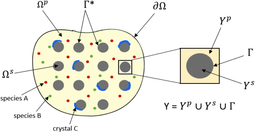
In this article, we consider an optimal control problem associated to a chemical transportation phenomena in a porous medium Ω. Let two mobile chemical species A, B are present in the porous part $(Ω^{p})$ and a crystal C is present on the surface $(Γ^{*})$ of solid matrices (see Fig. 1). They are connected via following reaction $\begin{matrix} A + B \to C . \end{matrix}$ This optimal control problem is concerned with the minimization of a cost functional $J_{i}$ , where $\begin{matrix} J_{i} (u_{i}, θ_{i}) = \frac{1}{2} \int_{S \times Ω^{p}} | u_{i} - u_{d_{i}} |^{2} d (x, t) + \frac{β}{2} \int_{S \times Ω^{p}} | θ_{i} |^{2} d (x, t) + \frac{1}{2} \int_{Ω^{p}} {| u_{i} (T, x) - u_{d_{i}} (T, x) |}^{2} d x \end{matrix}$ and subject to the state equations $\begin{aligned} (1.1a) & \frac{\partial u_{i}}{\partial t} + \nabla \cdot (- D_{i} \nabla u_{i}) = u_{i} + θ_{i} in S \times Ω^{p}, \\ (1.1b) & - D_{i} \nabla u_{i} \cdot \vec{n} = 0 on S \times \partial Ω, \\ (1.1c) & - D_{i} \nabla u_{i} \cdot \vec{n} = \frac{\partial w}{\partial t} on S \times Γ^{*}, \\ (1.1d) & \frac{\partial w}{\partial t} = k u_{1} u_{2} on S \times Γ^{*}, \\ (1.1e) & u_{i} (0, x) = u_{i_{0}} (x) in Ω, \\ (1.1f) & w (0, x) = w_{0} (x) on Γ^{*}, \end{aligned}$ where $u_{1}$ , $u_{2}$ and w are the concentrations of A, B and C, respectively. For $i = 1, 2$ , with the control variables $θ_{i} (\subset U_{i})$ , we aim to achieve the given desired states $u_{d_{i}}$ in $L^{2}$ -sense, where $U_{i}$ is a closed convex subset of $L^{2} (S \times Ω)$ . In general, the control variable $θ_{i}$ acts like either a source or a sink term in the optimal control problem. In the context of our problem, when $θ_{i} > 0$ , we inject chemical agent from outside and $θ_{i} < 0$ means extraction of chemical species from the system.

In this article our main objective is to find a control (optimal), which minimizes the cost functional $J_{i}$ . Later this minimization analysis leads us to a relation between optimal control and the corresponding adjoint state. We start with a microscopic description of the controlled system (see (1.2a)–(1.2f)). Then, we upscale the system to a macroscopic description via periodic homogenisation. For the existence of the solution of the controlled system (state equations), we use some fixed point techniques shown in [12,20]. Unfortunately, we are unable to find the positiveness of the solution as the nature of the control variable in terms of positiveness is completely unknown to us. For homogenisation part, we assume that the porous medium has periodic structure to avoid the geometric complexity. We first obtain an anticipated macro-structure by asymptotic expansion method see [16], although we also use rigorous two-scale convergence method and periodic unfolding method, cf. [1,8,14,23,25,26] and references therein. The two-scale convergence of the nonlinear term on boundary is not straightforward and required some delicate tools to deal with it. Final aim of this paper is to show the convergence of optimal solution (optimal control and the corresponding state) from microscopic to macroscopic description (see Theorem 2.3). Now, we move to the next section to get familiar with the microscopic description.

Fig. 1.

Mobile species A and B in $Ω^{p}$ with crystal C on $Γ^{*}$ .

1.1. Micro-model equation

Let $Ω \subset R^{n} (n = 2, 3)$ be a bounded porous medium with the pore space $Ω^{p}$ and union of the boundary of solid parts $Ω^{s}$ such that $Ω : = Ω^{p} \cup Ω^{s}$ , $Ω^{s} \cap {\bar{Ω}}^{p} = ϕ$ . Let $Γ^{*}$ and $\partial Ω$ denote the union of the boundaries of solid parts and the boundary of the domain, respectively. Further assume that domain Ω is periodic and covered by finitely many unit representative cells $Y : = {(0, 1)}^{n} \subset R^{n}$ , where Y is composed of $Y^{s}$ (solid part) with boundary Γ and $Y^{p}$ (pore part) such that $Y = Y^{s} \cup Y^{p}$ and $Γ = Y^{s} \cap {\bar{Y}}^{p}$ . For $k \in Z^{n}$ , $Y_{k} : = Y + k$ , $Y_{k}^{s} : = Y^{s} + k$ , $Y_{k}^{p} : = Y^{p} + k$ and $Γ_{k} : = Γ + k$ such that $Ω \subset ⋃_{k \in Z^{n}} Y_{k}$ , $Ω^{p} \subset ⋃_{k \in Z^{n}} Y_{k}^{p}$ , $Ω^{s} \subset ⋃_{k \in Z^{n}} Y_{k}^{s}$ , $Γ^{*} \subset ⋃_{k \in Z^{n}} Γ_{k}$ . To avoid technical glitch, we assume that the solids parts do not touch the boundary $\partial Ω$ as well as the boundary of Y. Let $ε > 0$ be the scale parameter and Ω be covered by a finite union of $ε Y_{k}$ cells such that $ε Y_{k} \subset Ω$ for $k \in Z^{n}$ , $Ω_{p}^{ε} : = ⋃_{k \in Z^{n}} {ε Y_{k}^{p} : ε Y_{k}^{p} \subset Ω}$ , $Ω_{s}^{ε} : = ⋃_{k \in Z^{n}} {ε Y_{k}^{s} : ε Y_{k}^{s} \subset Ω}$ , $Γ_{ε}^{*} : = ⋃_{k \in Z^{n}} {ε Γ_{k} : ε Γ_{k} \subset Ω} and \partial Ω_{p}^{ε} : = \partial Ω \cup Γ_{ε}^{*}$ . Also, $χ^{ε} (x) = χ (\frac{x}{ε})$ is defined by $χ^{ε} (x) = 1 for x \in Ω_{p}^{ε} and = 0 for x \in Ω - Ω_{p}^{ε}$ . We denote by $d x$ and $d y$ the volume elements in Ω and Y, and by $d σ_{y}$ and $d σ_{x}$ the surface elements on Γ and $Γ_{ε}^{*}$ , respectively. $S : = [0, T)$ , $T > 0$ denotes the time interval. Now, let the microscopic concentrations of A, B and C are $u_{1}^{ε}$ , $u_{2}^{ε}$ and $w_{ε}$ , respectively. Further assuming that there is no interaction happening between the chemical species on the outer boundary $\partial Ω$ and precipitation of crystal forms on the solid matrices $Γ_{ε}^{*}$ at pore scale level. Then $\begin{aligned} (1.2a) & \frac{\partial u_{i}^{ε}}{\partial t} + \nabla \cdot (- D_{i} \nabla u_{i}^{ε}) = u_{i}^{ε} + θ_{i}^{ε} in S \times Ω_{p}^{ε}, \\ (1.2b) & - D_{i} \nabla u_{i}^{ε} \cdot \vec{n} = 0 on S \times \partial Ω, \\ (1.2c) & - D_{i} \nabla u_{i}^{ε} \cdot \vec{n} = ε \frac{\partial w_{ε}}{\partial t} on S \times Γ_{ε}^{*}, \\ (1.2d) & \frac{\partial w_{ε}}{\partial t} = k u_{1}^{ε} u_{2}^{ε} on S \times Γ_{ε}^{*}, \\ (1.2e) & u_{i}^{ε} (0, x) = u_{i_{0}} (x) in Ω_{p}^{ε}, \\ (1.2f) & w_{ε} (0, x) = w_{0} (x) on Γ_{ε}^{*}, \end{aligned}$ where $D_{i}$ are the diffusion coefficients and $θ_{i}^{ε}$ are distributed control variable for concentrations $u_{i}^{ε}$ for $i = 1, 2$ , k is the precipitation rate constant. We denote (1.2a)–(1.2f) by $(P^{ε})$ . Let $U_{i}^{ε} \subset L^{2} (S \times Ω_{p}^{ε})$ be closed convex, called admissible control set. For $θ^{ε} = (θ_{1}^{ε}, θ_{2}^{ε}) \in U_{1}^{ε} \times U_{2}^{ε}$ , let a cost functional defined by $\begin{aligned} J_{i}^{ε} (θ_{i}^{ε}) & = \frac{1}{2} \int_{S \times Ω_{p}^{ε}} {| u_{i}^{ε} - u_{d_{i}} |}^{2} d (x, t) \\ (1.3) & + \frac{β}{2} \int_{S \times Ω_{p}^{ε}} {| θ_{i}^{ε} |}^{2} d (x, t) + \frac{1}{2} \int_{Ω_{p}^{ε}} {| u_{i}^{ε} (T, x) - u_{d_{i}} (T, x) |}^{2} d x \end{aligned}$ Where $β > 0$ and $u^{ε} = (u_{1}^{ε} (θ_{1}^{ε}), u_{2}^{ε} (θ_{2}^{ε}), w_{ε})$ is a solution of the problem (1.2a)–(1.2f). An optimal control problem $(O P^{ε})$ is to find ${min}_{θ_{i}^{ε} \in U_{i}^{ε}} J_{i}^{ε} (θ_{i}^{ε})$ , where $(u_{1}^{ε} (θ_{1}^{ε}), u_{2}^{ε} (θ_{2}^{ε}), w_{ε})$ is the solution of (1.2a)–(1.2f) and $i = 1, 2$ . Our main goal is to do the limiting analysis of $(O P^{ε})$ .

The brief layout of this paper is as follows: in Section 2, we state our main theorems and collect all the necessary mathematical tools for our proposed problems. In Section 3, we obtain the existence of the solution of the diffusion–reaction–precipitation system $P^{ε}$ (Theorem 2.1). The existence of optimal control and its characterization are studied in Section 4 (Theorem 2.2). In Section 5, we obtain an anticipated upscaled model by asymptotic expansion method. Then we study the limiting analysis and the convergence theorem (Theorem 2.3) in Section 6.

2. Mathematical preliminaries and problems description

Let $δ \in [0, 1]$ and $1 ⩽ ρ$ , $μ ⩽ \infty$ be such that $\frac{1}{ρ} + \frac{1}{μ} = 1$ . Assume that $Θ \in {Ω, Ω_{p}^{ε}}$ and $r \in N_{0}$ , then the standard notations $L^{ρ} (Θ)$ and $H^{r, ρ} (Θ)$ denote the Lebesgue space and Sobolev space with their usual norms. For $ρ = 2$ , we denote $H^{1, 2} (Θ) = H^{1} (Θ)$ . Similarly, $C^{δ} (\bar{Θ})$ , ${(\cdot, \cdot)}_{δ, r}$ and ${[\cdot, \cdot]}_{δ}$ are the Hölder, real- and complex-interpolation spaces respectively endowed with their standard norms, for definition confer [13,18]. $C_{p e r}^{β} (Y)$ denotes the set of all Y-periodic β-times continuously differentiable functions in y for $β \in N$ . The symbol ${(\cdot, \cdot)}_{H}$ represents the inner product on a Hilbert space H and $‖ \cdot ‖_{H}$ denotes the corresponding norm. For a Banach space X, $X^{*}$ denotes its dual and the duality pairing is denoted by ${⟨ \cdot, \cdot ⟩}_{X^{*} \times X}$ . Since $C_{0}^{\infty} (Θ)$ is space of all continuously differentiable functions with compact support in Θ, then the closure of $C_{0}^{\infty} (Θ)$ is $H_{0}^{1} (Θ)$ . The symbols ↪, $↪ ↪$ and $d_{↪}$ denote the continuous, compact and dense embeddings respectively. we define the function spaces $F^{ε} = {c^{ε} : c^{ε} \in L^{2} (S; H^{1} (Ω_{p}^{ε})), \partial_{t} c^{ε} \in L^{2} (S; H^{1} {(Ω_{p}^{ε})}^{*})}$ , $F = {c : c \in L^{2} (S; H^{1} (Ω)), \partial_{t} c \in L^{2} (S; H^{1} {(Ω)}^{*})}$ , $W_{ε} = {w_{ε} : w_{ε} \in L^{2} (S; L^{2} (Γ_{ε}^{*}), \partial_{t} w_{ε} \in L^{2} (S; L^{2} (Γ_{ε}^{*}))}$ and $W = {w : w \in L^{2} (S \times Ω \times Γ), \partial_{t} w \in L^{2} (S \times Ω \times Γ)}$ . We make the following assumptions for the sake of analysis of $P^{ε}$ .

$u_{i_{0}} (x) ⩾ 0$ and $w_{0} (x) ⩾ 0$ .

$u_{i_{0}} \in H^{1} (Ω)$ , $w_{0} \in L^{2} (Ω \times Γ)$ such that ${sup}_{ε > 0} {‖ u_{i_{0}} ‖}_{H^{1} (Ω)} < \infty$ and ${sup}_{ε > 0} {‖ w_{0} ‖}_{L^{2} (Ω \times Γ)} < \infty$ .

$θ_{i}^{ε} \in U_{i}^{ε} \subset L^{2} (S \times Ω_{p}^{ε})$ such that ${sup}_{ε > 0} {‖ θ_{i}^{ε} ‖}_{L^{2} (S \times Ω_{p}^{ε})} < \infty$ .

Nonlinear precipitation term is bounded in $L^{2} (S \times Γ_{ε}^{*})$ .

Constants $k, D_{i}, β > 0$ .

2.1. Weak formulation of (1.2a)–(1.2f)

Let the assumption A1–A5 be satisfied. A triplet $(u_{1}^{ε}, u_{2}^{ε}, w_{ε}) \in F^{ε} \times F^{ε} \times W_{ε}$ is said to be weak solution of (1.2a)–(1.2f) such that $(u_{1}^{ε}, u_{2}^{ε}, w_{ε}) (0, x) = (u_{1_{0}}, u_{2_{0}}, w_{0}) (x)$ for all $x \in Ω_{p}^{ε}$ , and $\begin{aligned} \int_{S} {⟨ \frac{\partial u_{i}^{ε} (t)}{\partial t}, η_{i} (t) ⟩}_{H^{1} {(Ω_{p}^{ε})}^{*} \times H^{1} (Ω_{p}^{ε})} d t + \int_{S \times Ω_{p}^{ε}} D_{i} \nabla u_{i}^{ε} \cdot \nabla η_{i} d (x, t) + ε \int_{S \times Γ_{ε}^{*}} \frac{\partial w_{ε}}{\partial t} η_{i} d (σ_{x}, t) \\ (2.1a) & = \int_{S \times Ω_{p}^{ε}} (u_{i}^{ε} + θ_{i}^{ε}) η_{i} d (x, t), \\ (2.1b) & \int_{S \times Γ_{ε}^{*}} \frac{\partial w_{ε}}{\partial t} ψ d (σ_{x}, t) = k \int_{S \times Γ_{ε}^{*}} u_{1}^{ε} u_{2}^{ε} ψ d (σ_{x}, t), \end{aligned}$ for all $η_{i} \in L^{2} (S; H^{1} (Ω_{p}^{ε}))$ , $ψ \in L^{2} (S; L^{2} (Γ_{ε}^{*}))$ and $i = 1, 2$ .

We are now going to state main theorems of this paper which are given below. From time to time, we will use the notation, $u_{i}^{ε *} (t, x) = u_{i}^{ε} ({(θ_{i}^{ε} (t, x))}^{*})$ , $θ_{i}^{ε *} (t, x) = {(θ_{i}^{ε} (t, x))}^{*}$ , $u_{i}^{0 *} (t, x) = u_{i}^{0} ({(θ_{i}^{0} (t, x))}^{*})$ and $θ_{i}^{0 *} (t, x) = {(θ_{i}^{0} (t, x))}^{*}$ , where ∗ is used in the sense of optimality.

Theorem 2.1.
Let the assumption A1–A5 be satisfied, then there exists a unique weak solution $(u_{1}^{ε}, u_{2}^{ε}, w_{ε}) \in F^{ε} \times F^{ε} \times W_{ε}$ of $(P^{ε})$ which satisfies $\begin{aligned} (2.2a) & {‖ u_{i}^{ε} (t) ‖}_{L^{2} (Ω_{p}^{ε})} ⩽ M_{i}, \\ (2.2b) & {‖ w_{ε} (t) ‖}_{L^{2} (Γ_{ε}^{})} ⩽ M_{3}, \\ (2.2c) & {‖ u_{i}^{ε} ‖}_{L^{2} (S \times Ω_{p}^{ε})} + {‖ \nabla u_{i}^{ε} ‖}_{L^{2} (S \times Ω_{p}^{ε})} + {‖ \partial_{t} u_{i}^{ε} ‖}_{L^{2} (S; H^{1} {(Ω_{p}^{ε})}^{})} < \infty, \\ (2.2d) & ‖ w_{ε} ‖_{L^{2} (S \times Γ_{ε}^{})} + ‖ \partial_{t} w_{ε} ‖_{L^{2} (S \times Γ_{ε}^{})} < \infty, \end{aligned}$ for a.e. $t \in S$ , $M_{i}$ ’s are constants independent of ε and $i = 1, 2$ .
Theorem 2.2.
Let the assumptions A1–A5 hold true. If $(u_{1}^{ε}, u_{2}^{ε}, w_{ε}) \in F^{ε} \times F^{ε} \times W_{ε}$ is the solution of the problem $(O P^{ε})$ , then, the optimal control, ${(θ_{i}^{ε} (t, x))}^{} = - \frac{1}{β} γ_{i}^{ε} (t, x)$ , where* $γ_{i}^{ε}$ is the solution of adjoint problem $\begin{aligned} (2.3a) & \partial_{t} γ_{i}^{ε} + D_{i} Δ γ_{i}^{ε} + γ_{i}^{ε} = u_{d_{i}} - u_{i}^{ε } in S \times Ω_{p}^{ε}, \\ (2.3b) & - D_{i} \nabla γ_{i}^{ε} \cdot \vec{n} = 0 on S \times \partial Ω, \\ (2.3c) & - D_{i} \nabla γ_{i}^{ε} \cdot \vec{n} = k ε u_{j}^{ε} γ_{i}^{ε} on S \times Γ_{ε}^{}, \\ (2.3d) & γ_{i}^{ε} (T, x) = u_{i}^{ε } (T, x) - u_{d_{i}} (T, x) in Ω_{p}^{ε}, \end{aligned}$ for i, j* = 1, 2 (i ≠ j) and it satisfies the optimality condition $\begin{aligned} (2.4) & \int_{S \times Ω_{p}^{ε}} (γ_{i}^{ε} + β θ_{i}^{ε }) (θ_{i}^{ε} - θ_{i}^{ε }) d (x, t) ⩾ 0 \end{aligned}$ Conversely, if $(u_{1}^{ε}, u_{2}^{ε}, w_{ε}) \in F^{ε} \times F^{ε} \times W_{ε}$ and $γ_{i}^{ε} \in F^{ε}$ solve the system $\begin{aligned} (2.5a) & \partial_{t} u_{i}^{ε} + \nabla \cdot (- D_{i} \nabla u_{i}^{ε}) = u_{i}^{ε} - \frac{1}{β} γ_{i}^{ε} in S \times Ω_{p}^{ε}, \\ (2.5b) & - D_{i} \nabla u_{i}^{ε} \cdot \vec{n} = 0 on S \times \partial Ω, \\ (2.5c) & - D_{i} \nabla u_{i}^{ε} \cdot \vec{n} = ε \frac{\partial w_{ε}}{\partial t} on S \times Γ_{ε}^{}, \\ (2.5d) & \frac{\partial w_{ε}}{\partial t} = k u_{1}^{ε} u_{2}^{ε} on S \times Γ_{ε}^{}, \\ (2.5e) & u_{i}^{ε} (0, x) = u_{i_{0}} (x) in Ω_{p}^{ε}, \\ (2.5f) & w_{ε} (0, x) = w_{0} (x) on Γ_{ε}^{}, \end{aligned}$ and* $\begin{aligned} (2.6a) & \partial_{t} γ_{i}^{ε} + D_{i} Δ γ_{i}^{ε} + γ_{i}^{ε} = u_{d_{i}} - u_{i}^{ε } in S \times Ω_{p}^{ε}, \\ (2.6b) & - D_{i} \nabla γ_{i}^{ε} \cdot \vec{n} = 0 on S \times \partial Ω, \\ (2.6c) & - D_{i} \nabla γ_{i}^{ε} \cdot \vec{n} = k ε u_{j}^{ε} γ_{i}^{ε} on S \times Γ_{ε}^{}, \\ (2.6d) & γ_{i}^{ε} (T, x) = u_{i}^{ε } (T, x) - u_{d_{i}} (T, x) in Ω_{p}^{ε}, \end{aligned}$ for i, j* = 1, 2 and $i \neq j$ . Then, $(u_{1}^{ε}, u_{2}^{ε}, w_{ε})$ is the optimal solution of $(O P^{ε})$ .

The homogenised problem $(OP)$ , is given by: find the ${min}_{θ_{i}^{0} \in U_{i}} J_{i}^{0} (θ_{i}^{0})$ , where $(u_{1}^{0}, u_{2}^{0}, w_{0})$ is the solution of the problem $\begin{aligned} (2.7a) & \partial_{t} u_{i}^{0} + \nabla \cdot (- A_{i} \nabla u_{i}^{0}) + P (t, x) = u_{i}^{0} + \bar{θ_{i}^{0}} in S \times Ω, \\ (2.7b) & - A_{i} \nabla u_{i}^{0} \cdot \vec{n} = 0 on S \times \partial Ω, \\ (2.7c) & \frac{\partial w_{0}}{\partial t} = k u_{1}^{0} u_{2}^{0} in S \times Ω \times Γ, \\ (2.7d) & u_{i}^{0} (0, x) = u_{i_{0}} (x) in Ω, \\ (2.7e) & w_{0} (0, x) = w_{0} (x) on Ω \times Γ, \end{aligned}$ where $P (t, x) = \frac{1}{| Y^{p} |} \int_{Γ} \frac{\partial w_{0}}{\partial t} d σ_{y}$ , $A_{i}$ are upscaled form of $D_{i}$ (see next theorem), $\bar{θ_{i}^{0}} = \frac{1}{| Y^{p} |} \int_{Y^{p}} θ_{i}^{0} d y$ and $i = 1, 2$ . The cost functional $J_{i}^{0}$ is given by $\begin{aligned} J_{i}^{0} (θ_{i}^{0}) & = \frac{1}{2} \int_{S \times Ω \times Y^{p}} {| u_{i}^{0} - u_{d_{i}} |}^{2} d (x, y, t) + \frac{β}{2 | Y^{p} |} \int_{S \times Ω \times Y^{p}} {| θ_{i}^{0} |}^{2} d (x, y, t) \\ (2.8) & + \frac{1}{2} \int_{Ω \times Y^{p}} {| u_{i}^{0} (T, x) - u_{d_{i}} (T, x) |}^{2} d (x, y) . \end{aligned}$ Theorem 2.3.
Let the assumptions $A 1 - A 5$ hold true. Then, there exists limit functions $u_{i}^{0}, γ_{i}^{0} \in F$ , $θ_{i}^{0} \in U_{i}$ of $u_{i}^{ε}$ , $γ_{i}^{ε}$ and $θ_{i}^{ε}$ for $i = 1, 2$ , defined in the sense of Lemma ( 6.3 ), such that $θ_{i}^{0 } = - \frac{1}{β} γ_{i}^{0}$ is the optimal control of the functional (* 2.8 ) and $γ_{i}^{0}$ is the solution of the (upscaled) adjoint problem $\begin{aligned} (2.9a) & \partial_{t} γ_{i}^{0} + \nabla_{x} \cdot (A_{i} \nabla_{x} γ_{i}^{o}) + γ_{i}^{0} + Q (t, x) = | Y^{p} | (u_{d_{i}} - u_{i}^{0 }) in S \times Ω, \\ (2.9b) & - A_{i} \nabla_{x} γ_{i}^{0} \cdot \vec{n} = 0 on S \times \partial Ω, \\ (2.9c) & γ_{i}^{0} (T, x) = | Y^{p} | (u_{i}^{0 } (T, x) - u_{d_{i}} (T, x)) in Ω, \end{aligned}$ where $\begin{aligned} (2.10) & \begin{aligned} A_{i} = {(a_{κ r}^{i})}_{1 ⩽ κ, r ⩽ n} = \int_{Y^{p}} \frac{D_{i}}{| Y^{p} |} (δ_{κ r} + \sum_{κ, r = 1}^{n} \frac{\partial l_{κ} (y)}{\partial y_{r}}) d y \\ and Q (t, x) = - \frac{1}{| Y^{p} |} \int_{Γ} k u_{j}^{0} (t, x) γ_{i}^{0} (t, x) d σ_{y} for i, j = 1, 2 (i \neq j) . \end{aligned} \end{aligned}$ Moreover, $\begin{array}{r} \int_{S \times Ω \times Y^{p}} (γ_{i}^{0} + β θ_{i}^{0 }) (θ_{i}^{0} - θ_{i}^{0 }) d (t, x, y) ⩾ 0 . \end{array}$ Conversely, if $(u_{1}^{0}, u_{2}^{0}, w_{0}, γ_{i}^{0}) \in F \times F \times W \times F$ solves the system $\begin{aligned} (2.11a) & \partial_{t} u_{i}^{0} + \nabla \cdot (- A_{i} \nabla u_{i}^{0}) + P (t, x) = u_{i}^{0} - \frac{1}{β} γ_{i}^{0} in S \times Ω, \\ (2.11b) & - A_{i} \nabla u_{i}^{0} \cdot \vec{n} = 0 on S \times \partial Ω, \\ (2.11c) & \partial_{t} w_{0} = k u_{1}^{0} u_{2}^{0} in S \times Ω \times Γ, \\ (2.11d) & u_{i}^{0} (0, x) = u_{i_{0}} (x) in Ω, \\ (2.11e) & w_{0} (0, x) = w_{0} (x) on Ω \times Γ \end{aligned}$ and $\begin{aligned} (2.12a) & \partial_{t} γ_{i}^{0} + \nabla_{x} \cdot (A_{i} \nabla_{x} γ_{i}^{0}) + γ_{i}^{0} + Q (t, x) = | Y^{p} | (u_{d_{i}} - u_{i}^{0 }) in S \times Ω, \\ (2.12b) & - A_{i} \nabla_{x} γ_{i}^{0} \cdot \vec{n} = 0 on S \times \partial Ω, \\ (2.12c) & γ_{i}^{0} (T, x) = | Y^{p} | (u_{i}^{0 } (T, x) - u_{d_{i}} (T, x)) in Ω, \end{aligned}$ then the triplet $(u_{1}^{0}, u_{2}^{0}, w_{0})$ solves the optimal control problem $(OP)$ .

3. Existence of solution of $P^{ε}$

Lemma 3.1.
For $i = 1, 2$ ; $u_{i}^{ε}$ satisfies the following estimate $\begin{aligned} (3.1) & {‖ u_{i}^{ε} ‖}_{L^{2} (S; L^{2} (Ω_{p}^{ε}))} + {‖ \nabla u_{i}^{ε} ‖}_{L^{2} (S; L^{2} (Ω_{p}^{ε}))} + {‖ \partial_{t} u_{i}^{ε} ‖}_{L^{2} (S; H^{1} {(Ω_{p}^{ε})}^{})} < \infty \end{aligned}$
Proof.
Choose $η_{i} = χ_{(0, t)} u_{i}^{ε} \in L^{2} (S; H^{1} (Ω_{p}^{ε}))$ as test function in the weak formulation (2.1a), then $\begin{aligned} \frac{1}{2} \int_{0}^{t} \frac{\partial}{\partial t} {‖ u_{i}^{ε} (t) ‖}_{L^{2} (Ω_{p}^{ε})}^{2} d t + \int_{0}^{t} D_{i} {‖ \nabla u_{i}^{ε} ‖}_{L^{2} (Ω_{p}^{ε})}^{2} d t + ε k \int_{0}^{t} \int_{Γ_{ε}^{}} u_{1}^{ε} u_{2}^{ε} u_{i}^{ε} d (σ_{x}, t) \\ = \int_{0}^{t} \int_{Ω_{p}^{ε}} {(u_{i}^{ε})}^{2} d (x, t) + \int_{0}^{t} \int_{Ω_{p}^{ε}} θ_{i}^{ε} u_{i}^{ε} d (x, t) \\ \Rightarrow {‖ u_{i}^{ε} (t) ‖}_{L^{2} (Ω_{p}^{ε})}^{2} + \int_{0}^{t} 2 D_{i} {‖ \nabla u_{i}^{ε} ‖}_{L^{2} (Ω_{p}^{ε})}^{2} d t \\ ⩽ {‖ u_{i_{0}} ‖}_{L^{2} (Ω_{p}^{ε})}^{2} + \int_{0}^{t} {‖ θ_{i}^{ε} (t) ‖}_{L^{2} (Ω_{p}^{ε}))}^{2} d t \\ (3.2) & + 3 \int_{0}^{t} {‖ u_{i}^{ε} ‖}_{L^{2} (Ω_{p}^{ε})}^{2} d t + ε k {\frac{1}{4 γ} \int_{0}^{t} {‖ u_{1}^{ε} u_{2}^{ε} ‖}_{L^{2} (Γ_{ε}^{})}^{2} d t + γ \int_{0}^{t} {‖ u_{i}^{ε} ‖}_{L^{2} (Γ_{ε}^{})}^{2} d t}, \end{aligned}$ where γ is the Young’s inequality constant. Now, by assumption A4 and the trace inequality Lemma A.2 on the boundary term ${‖ u_{i}^{ε} ‖}_{L^{2} (Γ_{ε}^{})}^{2}$ , we obtain $\begin{aligned} {‖ u_{i}^{ε} (t) ‖}_{L^{2} (Ω_{p}^{ε})}^{2} + 2 D_{i} \int_{0}^{t} {‖ \nabla u_{i}^{ε} ‖}_{L^{2} (Ω_{p}^{ε})}^{2} d t \\ ⩽ C_{1} + 3 \int_{0}^{t} {‖ u_{i}^{ε} (t) ‖}_{L^{2} (Ω_{p}^{ε})}^{2} d t + C γ {\int_{0}^{t} {‖ u^{ε} ‖}_{L^{2} (Ω_{p}^{ε})}^{2} d t + ε^{2} \int_{0}^{t} {‖ \nabla u_{i}^{ε} ‖}_{L^{2} (Ω_{p}^{ε})}^{2} d t} \\ (3.3) & = C_{1} + (3 + C γ) \int_{0}^{t} ‖ u_{i}^{ε} (t) ‖ |_{L^{2} (Ω_{p}^{ε})}^{2} d t + C γ ε^{2} \int_{0}^{t} {‖ \nabla u_{i}^{ε} ‖}_{L^{2} (Ω_{p}^{ε})}^{2} d t a.e. t \in S, \end{aligned}$ where C and $C_{1} (= {‖ u_{i_{0}} ‖}_{L^{2} (Ω_{p}^{ε})}^{2} + \int_{0}^{t} {‖ θ_{i}^{ε} (t) ‖}_{L^{2} (Ω_{p}^{ε}))}^{2} d t)$ are arbitrary constants independent of ε. As $0 < ε ≪ 1$ , this leads (3.3) to $\begin{aligned} (3.4) & {‖ u_{i}^{ε} (t) ‖}_{L^{2} (Ω_{p}^{ε})}^{2} + (2 D_{i} - C γ) \int_{0}^{t} {‖ \nabla u_{i}^{ε} ‖}_{L^{2} (Ω_{p}^{ε})}^{2} d t ⩽ C_{1} + (3 + C γ) \int_{0}^{t} {‖ u_{i}^{ε} (t) ‖}_{L^{2} (Ω_{p}^{ε})}^{2} d t . \end{aligned}$ We take $0 < γ < \frac{2 D_{i}}{C}$ , to obtain $\begin{matrix} {‖ u_{i}^{ε} (t) ‖}_{L^{2} (Ω_{p}^{ε})}^{2} ⩽ C_{1} + (2 D_{i} + 3) \int_{0}^{t} {‖ u_{i}^{ε} ‖}_{L^{2} (Ω_{p}^{ε})}^{2} d t . \end{matrix}$ □

Now, applying Gronwall’s inequality $\begin{matrix} (3.5) & {‖ u_{i}^{ε} (t) ‖}_{L^{2} (Ω_{p}^{ε})} ⩽ M_{i} < \infty a.e. t \in S . \end{matrix}$ Similarly for $0 < γ < \frac{2 D_{i}}{C}$ , estimate (3.4) implies $\begin{matrix} \int_{0}^{t} {‖ \nabla u_{i}^{ε} ‖}_{L^{2} (Ω_{p}^{ε})}^{2} d t < \infty . \end{matrix}$ Now for the remaining estimate, take an arbitrary $ψ (t) \in H^{1} (Ω_{p}^{ε})$ and by trace inequality Lemma A.2 $\begin{aligned} | ⟨ \partial_{t} u_{i}^{ε}, ψ ⟩ | & ⩽ D_{i} {‖ \nabla u_{i}^{ε} ‖}_{L^{2} (Ω_{p}^{ε})} ‖ \nabla ψ ‖_{L^{2} (Ω_{p}^{ε})} + ε ‖ \partial_{t} w_{ε} ‖_{L^{2} (Γ_{ε}^{})} ‖ ψ ‖_{L^{2} (Γ_{ε}^{})} \\ + ({‖ u_{i}^{ε} ‖}_{L^{2} (Ω_{p}^{ε})} + {‖ θ_{i}^{ε} ‖}_{L^{2} (Ω_{p}^{ε})}) ‖ ψ ‖_{L^{2} (Ω_{p}^{ε})} \\ ⩽ {D_{i} {‖ \nabla u_{i}^{ε} ‖}_{L^{2} (Ω_{p}^{ε})} + C_{2} ‖ \partial_{t} w_{ε} ‖_{L^{2} (Γ_{ε}^{})} + {‖ u_{i}^{ε} ‖}_{L^{2} (Ω_{p}^{ε})} + {‖ θ_{i}^{ε} ‖}_{L^{2} (Ω_{p}^{ε})}} ‖ ψ ‖_{H^{1} (Ω_{p}^{ε})}, \end{aligned}$ where $C_{2}$ is an arbitrary constant independent of ε, then it follows that $\begin{array}{r} {‖ \partial_{t} u_{i}^{ε} (t) ‖}_{H^{1} {(Ω_{p}^{ε})}^{}} ⩽ D_{i} {‖ \nabla u_{i}^{ε} ‖}_{L^{2} (Ω_{p}^{ε})} + C_{2} ‖ \partial_{t} w_{ε} ‖_{L^{2} (Γ_{ε}^{})} + {‖ u_{i}^{ε} ‖}_{L^{2} (Ω_{p}^{ε})} + {‖ θ_{i}^{ε} ‖}_{L^{2} (Ω_{p}^{ε})} for a.e. t \in S . \end{array}$ Hence from Lemma 3.2 required estimation can be derived. Lemma 3.2.
The solution $w_{ε}$ satisfies $‖ w_{ε} ‖_{L^{2} (S \times Γ_{ε}^{})}^{2} + ‖ \partial_{t} w_{ε} ‖_{L^{2} (S \times Γ_{ε}^{})}^{2} < \infty$ .
Proof.
Choose $ψ = χ_{(0, t)} w_{ε} \in L^{2} (S; L^{2} (Γ_{ε}^{}))$ as test function for (2.1b) and by the assumption A4, we obtain □
$\begin{aligned} (3.6) & {‖ w_{ε} (t) ‖}_{L^{2} (Γ_{ε}^{})}^{2} ⩽ C_{3} + \frac{k}{2} \int_{0}^{t} ‖ w_{ε} ‖_{L^{2} (Γ_{ε}^{})}^{2} d t, \end{aligned}$ where $C_{3}$ is an arbitrary constant independent of ε. Then Gronwall’s inequality leads (3.4) to $\begin{matrix} {‖ w_{ε} (t) ‖}_{L^{2} (Γ_{ε}^{})} ⩽ M_{3} < \infty a.e. t \in S . \end{matrix}$ Next choose $ψ = χ_{(0, t)} \partial_{t} w_{ε} \in L^{2} (S; L^{2} (Γ_{ε}^{}))$ as test function for (2.1b) to get the remaining estimate.

Now, we obtain the solution of $P^{ε}$ . Let consider the following closed and convex sets $\begin{aligned} X_{F^{ε}}^{1} = {u_{1}^{ε} \in F^{ε} : {‖ u_{1}^{ε} (t) ‖}_{L^{2} (Ω_{p}^{ε})} ⩽ M_{1} a.e. in S}, \\ X_{F^{ε}}^{2} = {u_{2}^{ε} \in F^{ε} : {‖ u_{2}^{ε} (t) ‖}_{L^{2} (Ω_{p}^{ε})} ⩽ M_{2} a.e. in S}, \\ X_{W_{ε}} = {w_{ε} \in W_{ε} : {‖ w_{ε} (t) ‖}_{L^{2} (Γ_{ε}^{})} ⩽ M_{3} a.e. in S} . \end{aligned}$ Existence of solution of (2.1a)–(2.1b) is motivated from nested concept of Banach fixed Point theorem, cf. Theorem 3.1 in [6] and Lemma 3.80 in [17]. The statement is: for arbitrary $(u_{1}^{ε}, u_{2}^{ε}) \in X_{F^{ε}}^{1} \times X_{F^{ε}}^{2}$ , consider the equation (2.1b) with $w_{ε} (0, x) = w_{0} (x)$ , then by Picard–Lindelöf theorem there exists a unique solution $w_{ε} \in X_{W_{ε}}$ of (2.1b), since r.h.s. of (2.1b) is Lipschitz. Again for $u_{1}^{ε} \in X_{F^{ε}}^{1}$ and (2.1a) with $u_{2}^{ε} (0, x) = u_{2_{0}}$ has a unique solution $T_{1} u_{2}^{ε} \in X_{F^{ε}}^{2}$ where $T_{1} : X_{F^{ε}}^{2} \to X_{F^{ε}}^{2}$ is a contraction map with unique fixed point in $X_{F^{ε}}^{2}$ . In this way, for $u_{1}^{ε} \in X_{F^{ε}}^{1}$ ; the equation (2.1a) has solution $T_{2} u_{1}^{ε}$ where $T_{2} : X_{F^{ε}}^{1} \to X_{F^{ε}}^{1}$ is a contraction map and has a fixed point in $X_{F^{ε}}^{1}$ . Clearly these fixed points of contraction maps define a solution of (2.1a)–(2.1b).
Lemma 3.3.
$T_{1} u_{2}^{ε}$ satisfies the following estimate $\begin{matrix} {‖ T_{1} u_{2}^{ε} ‖}_{L^{2} (S \times Ω_{p}^{ε})} + {‖ \nabla T_{1} u_{2}^{ε} ‖}_{L^{2} (S \times Ω_{p}^{ε})} + {‖ \partial_{t} T_{1} u_{2}^{ε} ‖}_{L^{2} (S; H^{1} {(Ω_{p}^{ε})}^{})} < \infty . \end{matrix}$ Proof.
Proof follows the same pattern of Lemma* 3.1 . □

Let ${(u_{2}^{ε})}^{(1)}, {(u_{2}^{ε})}^{(2)} \in X_{F^{ε}}^{2}$ with ${(w_{ε})}^{(1)}, {(w_{ε})}^{(2)} \in X_{W_{ε}}$ be the corresponding solution of (2.1b). Further we denote $\begin{array}{r} V (u_{2}^{ε}, t) = {‖ u_{2}^{ε} ‖}_{L^{2} ((0, t); H^{1} (Ω_{p}^{ε}))}^{2} = {‖ u_{2}^{ε} ‖}_{L^{2} ((0, t) \times Ω_{p}^{ε})}^{2} + {‖ \nabla u_{2}^{ε} ‖}_{L^{2} ((0, t) \times Ω_{p}^{ε})}^{2} \end{array}$ By Trace inequality of $u_{2}^{ε}$ on $Γ_{ε}^{}$ (see Lemma A.2), we have $\begin{array}{r} {‖ u_{2}^{ε} ‖}_{L^{2} ((0, t) \times Γ_{ε}^{})}^{2} ⩽ C_{4} V (u_{2}^{ε}, t) for all u_{2}^{ε} \in L^{2} (S; H^{1} (Ω_{p}^{ε})) \end{array}$ where $C_{4}$ is independent of ε.
Lemma 3.4.
If ${(w_{ε})}^{(1)}$ , ${(w_{ε})}^{(2)}$ are two solutions of ( 2.1b ) and $w_{ε} = {(w_{ε})}^{(1)} - {(w_{ε})}^{(2)}$ then for a.e. $t \in S$ we have, $\begin{aligned} ‖ w_{ε} ‖_{L^{2} ((0, t) \times Γ_{ε}^{})}^{2} ⩽ C_{5} V (u_{2}^{ε}, t) (e^{t} - 1) and ‖ \partial_{t} w_{ε} ‖_{L^{2} ((0, t) \times Γ_{ε}^{})}^{2} ⩽ C_{5} V (u_{2}^{ε}, t) \end{aligned}$ where $C_{5} = k^{2} L_{R_{1}}^{2} C_{4}$ , $C_{4}$ is the trace inequality constant and $L_{R_{1}}$ is the Lipschitz constant.
Proof.
Choose $ψ = χ_{(0, t)} w_{ε} \in L^{2} (S \times Γ_{ε}^{})$ as a test function in the weak formulation (2.1b), which yields $\begin{aligned} (3.7) & \frac{1}{2} \int_{0}^{t} \frac{\partial}{\partial t} ‖ w_{ε} ‖_{L^{2} (Γ_{ε}^{})}^{2} d t & = \int_{0}^{t} \int_{Γ_{ε}^{}} k u_{1}^{ε} {{(u_{2}^{ε})}^{(1)} - {(u_{2}^{ε})}^{(2)}} w_{ε} d (σ_{x}, t) . \end{aligned}$ Now locally Lipschitzness implies $\begin{aligned} (3.8) & {‖ w_{ε} (t) ‖}_{L^{2} (Γ_{ε}^{})}^{2} ⩽ 2 \int_{0}^{t} \int_{Γ_{ε}^{}} k L_{R_{1}} u_{2}^{ε} w_{ε} d (σ_{x}, t) \end{aligned}$ By Young’s inequality and Trace inequality of $u_{2}^{ε}$ on $Γ_{ε}^{}$ , we obtain $\begin{array}{r} 2 \int_{0}^{t} \int_{Γ_{ε}^{}} k L_{R_{1}} u_{2}^{ε} w_{ε} ⩽ k^{2} L_{R_{1}}^{2} C_{4} V (u_{2}^{ε}, t) + \int_{0}^{t} {‖ w_{ε} (t) ‖}_{L^{2} (Γ_{ε}^{})}^{2} d t . \end{array}$ Hence from (3.8), $\begin{aligned} (3.9) & {‖ w_{ε} (t) ‖}_{L^{2} (Γ_{ε}^{})}^{2} ⩽ C_{5} V (u_{2}^{ε}, t) + \int_{0}^{t} {‖ w_{ε} (t) ‖}_{L^{2} (Γ_{ε}^{})}^{2} d t where C_{5} = k^{2} L_{R_{1}}^{2} C_{4} . \end{aligned}$ By Gronwall’s inequality, (3.9) reads like $\begin{array}{r} {‖ w_{ε} (t) ‖}_{L^{2} (Γ_{ε}^{})}^{2} ⩽ C_{5} V (u_{2}^{ε}, t) e^{t} \Rightarrow {‖ w_{ε} (t) ‖}_{L^{2} ((0, t) \times Γ_{ε}^{})}^{2} ⩽ C_{5} V (u_{2}^{ε}, t) (e^{t} - 1) . \end{array}$

Again, choose $ψ = χ_{(0, t)} \partial_{t} w_{ε} \in L^{2} (S \times Γ_{ε}^{})$ as test function in (2.1b) and proceed in the similar fashion as above to get the estimate $‖ \partial_{t} w_{ε} ‖_{L^{2} ((0, t) \times Γ_{ε}^{})}^{2} ⩽ C_{5} V (u_{2}^{ε}, t)$ . □
Lemma 3.5.
For all $t \in S$ and $μ > 0$ (fixed) $\begin{aligned} {‖ T_{1} u_{2}^{ε} ‖}_{L^{2} ((0, t) \times Ω_{p}^{ε})}^{2} ⩽ \frac{μ C_{5} V (u_{2}^{ε}, t)}{2 (2 + \frac{2 C_{6}}{μ})} (e^{(2 + \frac{2 C_{6}}{μ}) t} - 1) and \\ {‖ \nabla T_{1} u_{2}^{ε} ‖}_{L^{2} ((0, t) \times Ω_{p}^{ε})}^{2} ⩽ \frac{μ C_{5} V (u_{2}^{ε}, t)}{2} e^{(2 + \frac{2 C_{6}}{μ}) t}, \end{aligned}$ where $C_{5} = k^{2} L_{R_{1}}^{2} C_{4}$ from Lemma 3.4 , $C_{6}$ and μ are the trace inequality and Young’s inequality constants, respectively such that $μ > \frac{C_{6}}{D_{2}}$ .
Proof.
Taking (2.1a) for the difference $T_{1} u_{2}^{ε} = T_{1} {(u_{2}^{ε})}^{(1)} - T_{1} {(u_{2}^{ε})}^{(2)}$ and choosing $η = χ_{(0, t)} T_{1} u_{2}^{ε}$ as test function for arbitrary $t \in S$ yields $\begin{aligned} \frac{1}{2} {‖ T_{1} u_{2}^{ε} (t) ‖}_{L^{2} (Ω_{p}^{ε})}^{2} + D_{2} \int_{0}^{t} {‖ \nabla T_{1} u_{2}^{ε} ‖}_{L^{2} (Ω_{p}^{ε})}^{2} & ⩽ \int_{0}^{t} {‖ T_{1} u_{2}^{ε} (t) ‖}_{L^{2} (Ω_{p}^{ε})}^{2} d t + \frac{ε μ}{4} \int_{0}^{t} ‖ \partial_{t} w_{ε} ‖_{L^{2} (Γ_{ε}^{})}^{2} d t \\ + \frac{ε}{μ} \int_{0}^{t} {‖ T_{1} u_{2}^{ε} (t) ‖}_{L^{2} (Γ_{ε}^{})}^{2} d t . \end{aligned}$ As $0 < ε ≪ 1$ , we have $\begin{array}{r} \frac{ε μ}{4} \int_{0}^{t} ‖ \partial_{t} w_{ε} ‖_{L^{2} (Γ_{ε}^{})}^{2} d t ⩽ \frac{C_{5} μ}{4} V (u_{2}^{ε}, t) (see Lemma 3.4), \end{array}$ and trace inequality A.2 gives $\begin{array}{r} ε {‖ T_{1} u_{2}^{ε} (t) ‖}_{L^{2} (Γ_{ε}^{})}^{2} ⩽ C_{6} {{‖ T_{1} u_{2}^{ε} (t) ‖}_{L^{2} (Ω_{p}^{ε})}^{2} + ε^{2} {‖ \nabla T_{1} u_{2}^{ε} ‖}_{L^{2} (Ω_{p}^{ε})}^{2}} . \end{array}$ Hence, we obtain $\begin{aligned} {‖ T_{1} u_{2}^{ε} (t) ‖}_{L^{2} (Ω_{p}^{ε})}^{2} + 2 D_{2} \int_{0}^{t} {‖ \nabla T_{1} u_{2}^{ε} ‖}_{L^{2} (Ω_{p}^{ε})}^{2} & ⩽ \frac{C_{5} μ}{2} V (u_{2}^{ε}, t) + (2 + \frac{2 C_{6}}{μ}) \int_{0}^{t} {‖ T_{1} u_{2}^{ε} (t) ‖}_{L^{2} (Ω_{p}^{ε})}^{2} d t \\ + \frac{2 C_{6}}{μ} \int_{0}^{t} {‖ \nabla T_{1} u_{2}^{ε} ‖}_{L^{2} (Ω_{p}^{ε})}^{2} d t . \end{aligned}$ Take $μ > \frac{C_{6}}{D_{2}}$ to get $\begin{array}{r} {‖ T_{1} u_{2}^{ε} (t) ‖}_{L^{2} (Ω_{p}^{ε})}^{2} ⩽ \frac{C_{5} μ}{2} V (u_{2}^{ε}, t) + (2 + \frac{2 C_{6}}{μ}) \int_{0}^{t} {‖ T_{1} u_{2}^{ε} (t) ‖}_{L^{2} (Ω_{p}^{ε})}^{2} d t . \end{array}$ Now, the monotonicity of $\frac{C_{5} μ}{2} V (u_{2}^{ε}, t)$ and integrating with respect to t forms the required first estimate and using this estimate we obtain the gradient estimate. □

Now, $\begin{aligned} V (T_{1} {(u_{2}^{ε})}^{(1)} - T_{1} {(u_{2}^{ε})}^{(2)}, t) & = {‖ T_{1} {(u_{2}^{ε})}^{(1)} - T_{1} {(u_{2}^{ε})}^{(2)} ‖}_{L^{2} ((0, t) \times Ω_{p}^{ε})}^{2} \\ + {‖ \nabla T_{1} {(u_{2}^{ε})}^{(1)} - \nabla T_{1} {(u_{2}^{ε})}^{(2)} ‖}_{L^{2} ((0, t) \times Ω_{p}^{ε})}^{2} \\ ⩽ {\frac{μ C_{5}}{2 (2 + \frac{2 C_{6}}{μ})} (e^{(2 + \frac{2 C_{6}}{μ}) t} - 1) + \frac{μ C_{5}}{2} e^{(2 + \frac{2 C_{6}}{μ}) t}} \\ \times V ({(u_{2}^{ε})}^{(1)} - {(u_{2}^{ε})}^{(2)}, t) \end{aligned}$ Putting $t = μ$ yields, $\begin{matrix} (3.10) & V (T_{1} {(u_{2}^{ε})}^{(1)} - T_{1} {(u_{2}^{ε})}^{(2)}, μ) ⩽ μ \tilde{C} V ({(u_{2}^{ε})}^{(1)} - {(u_{2}^{ε})}^{(2)}, μ), \end{matrix}$ where $\tilde{C} = \frac{C_{5}}{2 (2 + \frac{2 C_{6}}{μ})} (e^{(2 μ + 2 C_{6})} - 1) + \frac{C_{5}}{2} e^{(2 μ + 2 C_{6})}$ and the constants $C_{5}$ , $C_{6}$ are independent of the initial data. Hence, $\tilde{C}$ in (3.10), doesn’t depend on the initial data. Now if, $0 < μ \tilde{C} < 1$ i.e., $0 < \tilde{C} < \frac{1}{μ}$ , then $T_{1}$ becomes a contraction mapping on the closed set ${u_{2}^{ε} \in L^{2} ((0, μ); H^{1} (Ω_{p}^{ε})) : ‖ u_{2}^{ε} (μ) ‖ ⩽ M_{2}}$ and hence by Banach’s fixed point theorem $T_{1}$ has a fixed point $u_{2}^{ε}$ (say) in this set. By Lemma 3.3, $u_{2}^{ε} \in H^{1} ((0, μ); H^{1} {(Ω_{p}^{ε})}^{})$ and satisfies its a-priori estimates. Now, $u_{2}^{ε} \in C ([0, μ); L^{2} (Ω_{p}^{ε}))$ with $0 ⩽ ‖ u_{2}^{ε} ‖_{L^{2} (Ω_{p}^{ε})} ⩽ M_{2}$ . So, $u_{2}^{ε} (μ)$ can be used as initial condition for extending the time interval of existence. Since μ is independent of initial condition, we can get a fixed point of $T_{1}$ for a.e. $t \in S$ .
Lemma 3.6.
The fixed point* $u_{2}^{ε}$ of $T_{1}$ belongs to $X_{F^{ε}}^{2}$ exists uniquely and satisfies the following estimates $\begin{array}{r} {‖ u_{2}^{ε} ‖}_{L^{2} (S; L^{2} (Ω_{p}^{ε}))}^{2} + {‖ \nabla u_{2}^{ε} ‖}_{L^{2} (S; L^{2} (Ω_{p}^{ε}))}^{2} + {‖ \partial_{t} u_{2}^{ε} ‖}_{L^{2} (S; H^{1} {(Ω_{p}^{ε})}^{})}^{2} < \infty \end{array}$
Proof.
Assume that ${(u_{2}^{ε})}_{0}$ be an arbitrary and a sequence ${(u_{2}^{ε})}_{n} \in X_{F^{ε}}^{2} \cap H^{1} (S; H^{1} {(Ω_{p}^{ε})}^{})$ is constructed by the iterations ${(u_{2}^{ε})}_{n} = T_{1} {(u_{2}^{ε})}_{n - 1}$ , $n ⩾ 1$ , which becomes a Cauchy sequence in $X_{F^{ε}}^{2}$ . Now $X_{F^{ε}}^{2}$ is closed subspace in a Banach space and hence complete. So, there exists $u_{2}^{ε} \in X_{F^{ε}}^{2}$ such that ${(u_{2}^{ε})}_{n}$ converges to $u_{2}^{ε}$ as $n \to \infty$ . Again, $\begin{array}{r} V (T_{1} u_{2}^{ε} - u_{2}^{ε}, t) = V (lim_{n \to \infty} T_{1} {(u_{2}^{ε})}_{n} - u_{2}^{ε}, t) = V (lim_{n \to \infty} {(u_{2}^{ε})}_{n + 1} - u_{2}^{ε}, t) = V (u_{2}^{ε} - u_{2}^{ε}, t) = 0 \end{array}$ This implies $T_{1} u_{2}^{ε} = u_{2}^{ε}$ i.e., $u_{2}^{ε}$ is a fixed point of $T_{1}$ . For $0 < μ \tilde{C} < 1$ , $T_{1}$ is contraction map, hence it has a unique fixed point $u_{2}^{ε} \in X_{F^{ε}}^{2} \cap H^{1} (S; H^{1} {(Ω_{p}^{ε})}^{})$ . Now ${(u_{2}^{ε})}_{n}$ is uniformly bounded in $H^{1} (S; H^{1} {(Ω_{p}^{ε})}^{})$ hence, it has a weakly convergent subsequence ${(u_{2}^{ε})}_{n_{k}}$ with $u_{2}^{ε} \in H^{1} (S; H^{1} {(Ω_{p}^{ε})}^{})$ as a weak limit. By construction all ${(u_{2}^{ε})}_{n_{k}}$ satisfy the initial and boundary conditions and $\begin{aligned} \int_{S} {⟨ \frac{\partial {(u_{2}^{ε})}_{n_{k}}}{\partial t}, η ⟩}_{H^{1} {(Ω_{p}^{ε})}^{} \times H^{1} (Ω_{p}^{ε})} d t + \int_{S \times Ω_{p}^{ε}} D_{2} \nabla {(u_{2}^{ε})}_{n_{k}} \cdot \nabla η d (x, t) + \int_{S \times Γ_{ε}^{}} ε \frac{\partial {(w_{ε})}_{n_{k}}}{\partial t} η d (σ_{x}, t) \\ (3.11) & = \int_{S \times Ω_{p}^{ε}} ({(u_{2}^{ε})}_{n_{k}} + θ_{2}^{ε}) η d (x, t) \end{aligned}$ for all $η \in L^{2} (S; H^{1} (Ω_{p}^{ε}))$ and ${(w_{ε})}_{n_{k}}$ satisfies $\begin{aligned} (3.12) & \int_{S \times Γ_{ε}^{}} \frac{\partial {(w_{ε})}_{n_{k}}}{\partial t} ψ (t) d (σ_{x}, t) = k \int_{S \times Γ_{ε}^{}} u_{1}^{ε} {(u_{2}^{ε})}_{n_{k}} ψ d (σ_{x}, t) \end{aligned}$ for all $ψ \in L^{2} (S; L^{2} (Γ_{ε}^{}))$ with $w_{o}$ is initial data. By Lemma 3.4, the sequence ${(w_{ε})}_{n_{k}}$ converges strongly to a limit $w_{ε}$ in $H^{1} (S; L^{2} (Γ_{ε}^{}))$ . We can pass to the limit in (3.11) and (3.12) and then obtain $(u_{2}^{ε}, w_{ε})$ as a solution of the problem related to (2.1a)–(2.1b) for i=2.

$\underline{Uniqueness}$ : Let $({(u_{2}^{ε})}_{1}, {(w_{ε})}_{1})$ and $({(u_{2}^{ε})}_{2}, {(w_{ε})}_{2})$ be two solutions of the problem related to the equations (2.1a) and (2.1b). Assume $u_{2}^{ε} = {(u_{2}^{ε})}_{1} - {(u_{2}^{ε})}_{2}$ and $w_{ε} = {(w_{ε})}_{1} - {(w_{ε})}_{2}$ . By Lemma 3.4 $\begin{aligned} (3.13) & \begin{aligned} ‖ w_{ε} ‖_{L^{2} ((0, t) \times Γ_{ε}^{})}^{2} ⩽ k^{2} L_{R_{1}}^{2} {‖ u_{2}^{ε} ‖}_{L^{2} ((0, t) \times Γ_{ε}^{})}^{2} (e^{t} - 1) \\ ‖ \partial_{t} w_{ε} ‖_{L^{2} ((0, t) \times Γ_{ε}^{})} ⩽ k^{2} L_{R_{1}}^{2} {‖ u_{2}^{ε} ‖}_{L^{2} ((0, t) \times Γ_{ε}^{})}^{2} for a.e. t \in S . \end{aligned} \end{aligned}$ Now take $u_{2}^{ε}$ as test function in (2.1a) and using trace inequality, we obtain $\begin{array}{r} {‖ u_{2}^{ε} (t) ‖}_{L^{2} (Ω_{p}^{ε})}^{2} + 2 D_{2} {‖ \nabla u_{2}^{ε} ‖}_{L^{2} ((0, t) \times Ω_{p}^{ε})}^{2} ⩽ C_{7} \int_{0}^{t} {‖ u_{2}^{ε} (t) ‖}_{L^{2} (Ω_{p}^{ε})}^{2} + C_{8} \int_{0}^{t} {‖ \nabla u_{2}^{ε} (t) ‖}_{L^{2} (Ω_{p}^{ε})}^{2}, \end{array}$ where constants $C_{7}$ and $C_{8}$ are independent of ε. Setting $C_{8} = 2 D_{2}$ implies $‖ u_{2}^{ε} (t) ‖_{L^{2} (Ω_{p}^{ε})}^{2} ⩽ C_{7} \int_{0}^{t} ‖ u_{2}^{ε} (t) ‖_{L^{2} (Ω_{p}^{ε})}^{2}$ . Hence, from Gronwall’s inequality $\begin{array}{r} {‖ u_{2}^{ε} (t) ‖}_{L^{2} (Ω_{p}^{ε})}^{2} = 0 \Rightarrow {(u_{2}^{ε})}_{1} = {(u_{2}^{ε})}_{2} for a.e. t \in S . \end{array}$ From (3.13), we have $\begin{array}{r} {‖ w_{ε} (t) ‖}_{L^{2} (Γ_{ε}^{})}^{2} = 0 \Rightarrow {(w_{ε})}_{1} = {(w_{ε})}_{2} for a.e. t \in S . \end{array}$ □

Now for existence of solution of (2.1a) for $i = 1$ and (2.1b), define $T_{2} : X_{F^{ε}}^{1} \to X_{F^{ε}}^{1}$ contraction operator and proceed in the similar way as before. Remark 3.1.
Instead of considering the assumption A4, one can take polynomial type growth of the nonlinear precipitation term $(f (u_{1}^{ε}, u_{2}^{ε}) = k u_{1}^{ε} u_{2}^{ε})$ i.e., $\begin{matrix} | f (u_{1}^{ε}, u_{2}^{ε}) | ⩽ C (1 + {| u_{1}^{ε} |}^{γ_{1}} + {| u_{2}^{ε} |}^{γ_{2}}), \end{matrix}$ where $C > 0$ (independent of ε) and $0 ⩽ γ_{1}$ , $γ_{2} ⩽ 1$ (see [15,22,27]). Then, following in the similar fashion as in Lemmas 3.1 and 3.2, required estimates can be obtained. Indeed, for $i = 1, 2$ choose $η_{i} = χ_{(0, t)} u_{i}^{ε} \in L^{2} (S; H^{1} (Ω_{p}^{ε}))$ as test functions in the weak formulation (2.1a), then $\begin{aligned} \frac{d}{d t} {‖ u_{1}^{ε} ‖}_{L^{2} (Ω_{p}^{ε})}^{2} + (2 D_{1} - C_{1}) {‖ \nabla u_{1}^{ε} ‖}_{L^{2} (Ω_{p}^{ε})}^{2} \\ ⩽ (C_{1} + 2) {‖ u_{1}^{ε} ‖}_{L^{2} (Ω_{p}^{ε})}^{2} + C_{2} ({‖ u_{2}^{ε} ‖}_{L^{2} (Ω_{p}^{ε})}^{2} + {‖ \nabla u_{2}^{ε} ‖}_{L^{2} (Ω_{p}^{ε})}^{2}) \\ + C_{3}, \\ \frac{d}{d t} {‖ u_{2}^{ε} ‖}_{L^{2} (Ω_{p}^{ε})}^{2} + (2 D_{2} - C_{1}^{'}) {‖ \nabla u_{2}^{ε} ‖}_{L^{2} (Ω_{p}^{ε})}^{2} \\ ⩽ (C_{1}^{'} + 2) {‖ u_{2}^{ε} ‖}_{L^{2} (Ω_{p}^{ε})}^{2} + C_{2}^{'} ({‖ u_{1}^{ε} ‖}_{L^{2} (Ω_{p}^{ε})}^{2} + {‖ \nabla u_{1}^{ε} ‖}_{L^{2} (Ω_{p}^{ε})}^{2}) \\ + C_{3}^{'}, \end{aligned}$ where constants $C_{i}$ , $C_{i}^{'}$ are independent of ε. Now, adding the above inequalities and by the Gronwall’s inequality one can obtain the required estimates.

4. Optimality condition

Lemma 4.1.
There exist a unique $θ_{i}^{ε} \in U_{i}^{ε}$ such that the minimization problem $J_{i}^{ε}$ will attain it’s infimum.
Proof.
Let $m = {inf}_{θ_{i}^{ε} \in U_{i}^{ε}} J_{i}^{ε} (u_{i}^{ε} (θ_{i}^{ε}))$ . Since $0 ⩽ m < \infty$ , there exist a sequence ${(θ_{i}^{ε})}_{n} \in U_{i}^{ε} \subset L^{2} (S \times Ω_{p}^{ε})$ such that ${lim}_{n \to \infty} J_{i}^{ε} (u_{i}^{ε} ({(θ_{i}^{ε})}_{n})) = m$ . Without loss of generality, we can assume that $J_{i}^{ε} (u_{i}^{ε} ({(θ_{i}^{ε})}_{n})) ⩽ J_{i}^{ε} (u_{i}^{ε} (0))$ , then Lemma 3.1 implies ${‖ {(θ_{i}^{ε})}_{n} ‖}_{L^{2} (S \times Ω_{p}^{ε})} < \infty$ . Thus up to subsequence, there exists a subsequence of ${(θ_{i}^{ε})}_{n}$ , still indexed by n and a function $θ_{i}^{ε} \in L^{2} (S \times Ω_{p}^{ε})$ s.t. ${(θ_{i}^{ε})}_{n}$ converges to $θ_{i}^{ε}$ for the weak topology of $L^{2} (S \times Ω_{p}^{ε})$ . Using the fact the mapping ${‖ \cdot ‖}^{2}$ is weakly lower semi continuous in $L^{2} (S \times Ω_{p}^{ε})$ , then we have $\begin{aligned} (4.1) & {‖ θ_{i}^{ε} ‖}_{L^{2} (S \times Ω_{p}^{ε})}^{2} ⩽ \underset{n \to \infty}{lim inf} {‖ {(θ_{i}^{ε})}_{n} ‖}_{L^{2} (S \times Ω_{p}^{ε})}^{2} \end{aligned}$ Since $L^{2} (S \times Ω_{p}^{ε}) ∋ θ_{i}^{ε} \mapsto u_{i}^{ε} (θ_{i}^{ε}) \in F^{ε}$ is continuous and linear operator, $u_{i}^{ε}$ is also continuous in weak topology sense. This implies $u_{i}^{ε} ({(θ_{i}^{ε})}_{n})$ converges to $u_{i}^{ε} (θ_{i}^{ε})$ for the weak topology of $F^{ε}$ . Since $F^{ε} ↪ L^{2} (S \times Ω_{p}^{ε})$ compactly, $u_{i}^{ε} ({(θ_{i}^{ε})}_{n})$ converges to $u_{i}^{ε} (θ_{i}^{ε})$ for the weak topology of $L^{2} (S \times Ω_{p}^{ε})$ . Then $\begin{aligned} (4.2) & \int_{S \times Ω_{p}^{ε}} {| u_{i}^{ε} (θ_{i}^{ε}) - u_{d_{i}} |}^{2} ⩽ \underset{n \to \infty}{lim inf} \int_{S \times Ω_{p}^{ε}} {| u_{i}^{ε} ({(θ_{i}^{ε})}_{n}) - u_{d_{i}} |}^{2} \end{aligned}$ Combining (4.1) and (4.2) to get the existence of the optimal control problem ( $O P^{ε}$ ), i.e. $\begin{aligned} (4.3) & J_{i}^{ε} (u_{i}^{ε} (θ_{i}^{ε})) ⩽ \underset{n \to \infty}{lim inf} J_{i}^{ε} (u_{i}^{ε} ({(θ_{i}^{ε})}_{n})) = inf_{θ_{i}^{ε} \in U_{i}^{ε}} J_{i}^{ε} (u_{i}^{ε} (θ_{i}^{ε})) \end{aligned}$ The uniqueness follows from the convexity of $J_{i}^{ε}$ . □
Proof of Theorem 2.2.
Now, we obtain the optimality condition for microscopic description of the optimal control problem $({OP}^{ε})$ , which is motivated from [28].

Step 1. Let $F (θ_{i}^{ε}) = J_{i}^{ε} (u_{i}^{ε} (θ_{i}^{ε}), θ_{i}^{ε})$ . Then, by the optimality condition $\begin{matrix} \frac{1}{λ} [F (θ_{i}^{ε } + λ θ_{i}^{ε}) - F (θ_{i}^{ε })] ⩾ 0 for any θ_{i}^{ε} \in U_{i}^{ε} . \end{matrix}$ Here our aim is to find $\begin{matrix} lim_{λ \to 0} \frac{1}{λ} [F (θ_{i}^{ε } + λ θ_{i}^{ε}) - F (θ_{i}^{ε })] . \end{matrix}$ Now, $\begin{aligned} \frac{1}{λ} [F (θ_{i}^{ε } + λ θ_{i}^{ε}) - F ((θ_{i}^{ε }))] \\ = \frac{1}{2 λ} \int_{S \times Ω_{p}^{ε}} [{u_{i}^{ε} (θ_{i}^{ε } + λ θ_{i}^{ε}) - u_{i}^{ε} (θ_{i}^{ε })} {u_{i}^{ε} (θ_{i}^{ε } + λ θ_{i}^{ε}) + u_{i}^{ε} (θ_{i}^{ε }) - 2 u_{d_{i}}}] d (x, t) \\ + \frac{1}{2 λ} \int_{Ω_{p}^{ε}} [{u_{i}^{ε} (θ_{i}^{ε } (T) + λ θ_{i}^{ε} (T)) - u_{i}^{ε} (θ_{i}^{ε } (T))} \\ \times {u_{i}^{ε} (θ_{i}^{ε } (T) + λ θ_{i}^{ε} (T)) + u_{i}^{ε} (θ_{i}^{ε } (T)) - 2 u_{d_{i}} (T)}] d x \\ (4.4) & + \frac{β_{i}}{2 λ} \int_{S \times Ω_{p}^{ε}} [2 λ θ_{i}^{ε} θ_{i}^{ε } + λ^{2} {| θ_{i}^{ε} |}^{2}] d (x, t) . \end{aligned}$ Let ${(u_{i}^{ε})}_{λ} = u_{i}^{ε} (λ θ_{i}^{ε} + θ_{i}^{ε }, u_{i_{0}})$ , $u_{i}^{ε } = u_{i}^{ε} (θ_{i}^{ε }, u_{i_{0}})$ and ${(r_{i}^{ε})}_{λ} = {(u_{i}^{ε})}_{λ} - u_{i}^{ε }$ , then ${(r_{i}^{ε})}_{λ}$ is a solution of $\begin{aligned} (4.5a) & \frac{\partial {(r_{i}^{ε})}_{λ}}{\partial t} + \nabla \cdot (- D_{i} \nabla {(r_{i}^{ε})}_{λ}) = {(r_{i}^{ε})}_{λ} + λ θ_{i}^{ε} in S \times Ω_{p}^{ε}, \\ (4.5b) & - D_{i} \nabla {(r_{i}^{ε})}_{λ} \cdot \vec{n} = 0 on S \times \partial Ω, \\ (4.5c) & - D_{i} \nabla {(r_{i}^{ε})}_{λ} \cdot \vec{n} = ε k {(r_{i}^{ε})}_{λ} u_{j}^{ε} on S \times Γ_{ε}^{}, \\ (4.5d) & {(r_{i}^{ε})}_{λ} (0, x) = 0 in Ω_{p}^{ε} \end{aligned}$ Where $i, j = 1, 2$ and $i \neq j$ .

Now, we want to show that ${(u_{i}^{ε})}_{λ} \to u_{i}^{ε }$ in $F^{ε}$ as $λ \to 0$ . Choose ${(r_{i}^{ε})}_{λ}$ as test function in (4.5a), then using the assumption A4, trace inequality A.2 and Gronwall’s inequality, we obtain $\begin{aligned} (4.6) & {‖ \partial_{t} {(r_{i}^{ε})}_{λ} ‖}_{L^{2} (S; H^{1} {(Ω_{p}^{ε})}^{})} + {‖ {(r_{i}^{ε})}_{λ} ‖}_{L^{2} (S; H^{1} (Ω_{p}^{ε}))} ⩽ C | λ | {‖ θ_{i}^{ε} ‖}_{L^{2} (S \times Ω_{p}^{ε})} < \infty, \end{aligned}$ where constant C is independent of ε and this estimate implies the required limit. Now, set $r_{i}^{ε} = \frac{1}{λ} {(r_{i}^{ε})}_{λ}$ , then $r_{i}^{ε}$ is a solution of $\begin{aligned} (4.7a) & \frac{\partial r_{i}^{ε}}{\partial t} + \nabla \cdot (- D_{i} \nabla r_{i}^{ε}) = r_{i}^{ε} + θ_{i}^{ε} in S \times Ω_{p}^{ε} \\ (4.7b) & - D_{i} \nabla r_{i}^{ε} \cdot \vec{n} = 0 on S \times \partial Ω \\ (4.7c) & - D_{i} \nabla r_{i}^{ε} \cdot \vec{n} = ε k r_{i}^{ε} u_{j}^{ε} on S \times Γ_{ε}^{} \\ (4.7d) & r_{i}^{ε} (0, x) = 0 in Ω_{p}^{ε} \end{aligned}$ where $i, j = 1, 2$ and $i \neq j$ . We take limit on both sides of (4.4) $\begin{aligned} F^{'} (θ_{i}^{ε }) (θ_{i}^{ε}) & = lim_{λ \to 0} \frac{1}{λ} [F (θ_{i}^{ε } + λ θ_{i}^{ε}) - F (θ_{i}^{ε })] = \int_{S \times Ω_{p}^{ε}} (u_{i}^{ε } - u_{d_{i}}) r_{i}^{ε} d (x, t) \\ (4.8) & + \int_{Ω_{p}^{ε}} (u_{i}^{ε } (T, x) - u_{d_{i}} (T, x)) r_{i}^{ε} (T, x) d x + β \int_{S \times Ω_{p}^{ε}} θ_{i}^{ε } θ_{i}^{ε} d (x, t) \end{aligned}$ Now, if a $γ_{i}^{ε} \in F^{ε}$ is a solution of the adjoint system $\begin{aligned} (4.9a) & \partial_{t} γ_{i}^{ε} + D_{i} Δ γ_{i}^{ε} + γ_{i}^{ε} = u_{d_{i}} - u_{i}^{ε } in S \times Ω_{p}^{ε}, \\ (4.9b) & - D_{i} \nabla γ_{i}^{ε} \cdot \vec{n} = 0 on S \times \partial Ω, \\ (4.9c) & - D_{i} \nabla γ_{i}^{ε} \cdot \vec{n} = k ε u_{j}^{ε} γ_{i}^{ε} on S \times Γ_{ε}^{}, \\ (4.9d) & γ_{i}^{ε} (T, x) = u_{i}^{ε } (T, x) - u_{d_{i}} (T, x) in Ω_{p}^{ε}, \end{aligned}$ where $i, j = 1, 2$ and $i \neq j$ . Then from (4.8) and the adjoint system (4.9a)–(4.9d), we get $\begin{array}{r} F^{'} (θ_{i}^{ε }) (θ_{i}^{ε}) = \int_{S \times Ω_{p}^{ε}} θ_{i}^{ε} γ_{i}^{ε} d (x, t) + β \int_{S \times Ω_{p}^{ε}} θ_{i}^{ε } θ_{i}^{ε} d (x, t) = \int_{S \times Ω_{p}^{ε}} (γ_{i}^{ε} + β θ_{i}^{ε }) θ_{i}^{ε} d (x, t), \end{array}$ which gives the optimality condition as $\begin{matrix} \int_{S \times Ω_{p}^{ε}} (γ_{i}^{ε} + β θ_{i}^{ε }) (θ_{i}^{ε} - θ_{i}^{ε }) d (x, t) ⩾ 0 . \end{matrix}$ Furthermore, since $\begin{matrix} (4.10) & F^{'} (θ_{i}^{ε }) (θ_{i}^{ε}) = \int_{S \times Ω_{p}^{ε}} (γ_{i}^{ε} + β θ_{i}^{ε }) θ_{i}^{ε} d (x, t) = 0 \Rightarrow θ_{i}^{ε } (t, x) = - \frac{1}{β} γ_{i}^{ε} (t, x) . \end{matrix}$ Step 2. Existence of solution of ( 2.3a )–( 2.3d ) and ( 2.5a )–( 2.5f ): Note that PDE (2.3a)–(2.3d) is a terminal value problem (TVP). To show the existence of the solution of TVP, we substitute $v_{i}^{ε} (t, x) = γ_{i}^{ε} (T - t, x)$ , then $\begin{aligned} (4.11a) & - \partial_{t} v_{i}^{ε} + \nabla D_{i} \nabla v_{i}^{ε} + v_{i}^{ε} = u_{d_{i}} (T - t) - {(u_{i}^{ε})}^{} (T - t) in S \times Ω_{p}^{ε}, \\ (4.11b) & - D_{i} \nabla v_{i}^{ε} \cdot \vec{n} = 0 on S \times \partial Ω, \\ (4.11c) & - D_{i} \nabla v_{i}^{ε} \cdot \vec{n} = k ε u_{j}^{ε} (T - t) v_{i}^{ε} on S \times Γ_{ε}^{}, \\ (4.11d) & v_{i}^{ε} (0, x) = {(u_{i}^{ε})}^{} (T, x) - u_{d_{i}} (T, x) in Ω_{p}^{ε} . \end{aligned}$ Now, the existence of solution of above PDE is similar to the existence Theorem 2.1. Again, the existence of solution of (2.5a) together with boundary and initial conditions is directly follows from Theorem 2.1.

Step 3. Conversely: From the previous calculations, we have ${(θ_{i}^{ε} (t, x))}^{} = - \frac{1}{β} γ_{i}^{ε} (t, x)$ for every $θ_{i}^{ε} \in U_{i}^{ε} \subset L^{2} (S \times Ω_{p}^{ε})$ , where $γ_{i}^{ε}$ is the solution to the adjoint problem. Thus, if $(u_{1}^{ε}, u_{2}^{ε}, w_{ε}, γ_{i}^{ε}) \in F^{ε} \times F^{ε} \times W_{ε} \times F^{ε}$ satisfies the optimality system then we have $F^{'} (- \frac{1}{β} γ_{i}^{ε} (t, x)) = γ_{i}^{ε} (t, x) - β \frac{1}{β} γ_{i}^{ε} (t, x) = 0$ . Thus, it follows that $- \frac{1}{β} γ_{i}^{ε}$ is the optimal control to the problem $({OP}^{ε})$ . □
5. An anticipated macroscale model

In this section, we try to find an anticipated upscaled (macroscale) model of (1.2a)–(1.2f) and (2.3a)–(2.6d) by asymptotic expansion method (see [16]).

Let us take: (i) $u_{i}^{ε} (t, x) = Σ_{k = 0}^{\infty} ε^{k} u_{i}^{k} (t, x, y)$ ; (ii) $γ_{i}^{ε} (t, x) = Σ_{k = 0}^{\infty} ε^{k} γ_{i}^{k} (t, x, y)$ ; (iii) $θ_{i}^{ε} (t, x) = \sum_{k = 0}^{\infty} ε^{k} θ_{i}^{k} (t, x, y)$ ; (iv) $θ_{i}^{ε *} = {(θ_{i}^{ε} (t, x))}^{*} = \sum_{k = 0}^{\infty} ε^{k} {(θ_{i}^{*})}^{k} (t, x, y)$ ; (v) $w_{ε} (t, x) = Σ_{k = 0}^{\infty} ε^{k} w_{k} (t, x, y)$ , where each $u_{i}^{k}$ , $γ_{i}^{k}$ , $θ_{k}$ , $w_{k}$ and $θ_{k}^{*}$ are Y-periodic in y.

Step 1. For $i = 1, 2$ , from (1.2a) and (1.2c), we obtain $\begin{aligned} (5.1) & \frac{\partial}{\partial t} (\sum_{k = 0}^{\infty} ε^{k} u_{i}^{k}) - (\nabla_{x} + \frac{1}{ε} \nabla_{y}) \cdot {D_{i} (\nabla_{x} + \frac{1}{ε} \nabla_{y}) (\sum_{k = 0}^{\infty} ε^{k} u_{i}^{k})} = \sum_{k = 0}^{\infty} ε^{k} u_{i}^{k} + \sum_{k = 0}^{\infty} ε^{k} θ_{i}^{k} \\ (5.2) & - D_{i} (\nabla_{x} + \frac{1}{ε} \nabla_{y}) (\sum_{k = 0}^{\infty} ε^{k} u_{i}^{k}) \cdot \vec{n} = ε \frac{\partial}{\partial t} (\sum_{k = 0}^{\infty} ε^{k} w_{k}) . \end{aligned}$ Now comparing the coefficient of $ε^{- 2}$ on the both sides of (5.1) and the coefficient $ε^{- 1}$ on the both sides of (5.2), we get $\begin{aligned} (5.3) & \begin{aligned} \nabla_{y} \cdot (- D_{i} \nabla_{y} u_{i}^{0}) = 0 and - D_{i} \nabla_{y} u_{i}^{0} \cdot \vec{n} = 0 \\ \Rightarrow \int_{Y^{p}} D_{i} {| \nabla_{y} u_{i}^{0} (t, x, y) |}^{2} d y = 0 \Rightarrow {| \nabla_{y} u_{i}^{0} (t, x, y) |}^{2} = 0 \\ ⟹ u_{i}^{0} (t, x, y) = u_{i}^{0} (t, x) . \end{aligned} \end{aligned}$ Again, comparing the coefficients of $ε^{- 1}$ on both sides (5.1), we obtain $\begin{array}{r} \nabla_{y} \cdot (- D_{i} (\nabla_{x} u_{i}^{0} + \nabla u_{i}^{1})) = 0 ⟹ \nabla_{y} \cdot (\nabla_{y} u_{i}^{1}) = - \sum_{κ = 1}^{n} \frac{\partial}{\partial y_{κ}} (\frac{\partial u_{i}^{0}}{\partial x_{κ}}) . \end{array}$ This implies that $u_{i}^{1} (t, x, y) = \sum_{κ = 1}^{n} \frac{\partial u_{i}^{0} (t, x)}{\partial x_{κ}} l_{κ} (y) + c (x)$ , where, for each $κ = 1, 2, \dots, n$ ; $l_{κ} (y)$ is the Y-periodic solution of the cell problem $\begin{aligned} \nabla_{y} \cdot (\nabla_{y} l_{κ} + e_{κ}) & = 0 \forall y \in Y^{p} and (\nabla_{y} l_{κ} + e_{κ}) \cdot \vec{n} = 0 on Γ . \end{aligned}$ Further comparing the coefficients of $ε^{0}$ on both sides of (5.1) and integrating w.r.t. y to obtain $\begin{aligned} \int_{Y^{p}} {\frac{\partial u_{i}^{0}}{\partial t} - D_{i} Δ_{x} u_{i}^{0} + \nabla_{x} \cdot (- D_{i} \nabla_{y} u_{i}^{1}) + \nabla_{y} \cdot (- D_{i} \nabla_{x} u_{i}^{1}) + \nabla_{y} \cdot (- D_{i} \nabla_{y} u_{i}^{2})} d y \\ (5.4) & = \int_{Y^{p}} (u_{i}^{0} + θ_{i}^{0}) d y . \end{aligned}$ For more simplification of (5.4) we compare the coefficient of ε on both sides of (5.2) in order to obtain $- D_{i} (\nabla_{x} u_{i}^{1} + \nabla_{y} u_{i}^{2}) \cdot \vec{n} = \frac{\partial w_{0}}{\partial t}$ and this can be used to rewrite the integral $\begin{aligned} (5.5) & \int_{Y^{p}} (\nabla_{y} \cdot (- D_{i} \nabla_{x} u_{i}^{1} - D_{i} \nabla_{y} u_{i}^{2}) d y = - \int_{Γ} D_{i} (\nabla_{x} u_{i}^{1} + \nabla_{y} u_{i}^{2}) . \vec{n} d σ_{y} = \int_{Γ} \frac{\partial w_{0}}{\partial t} d σ_{y} . \end{aligned}$ Thus, (5.4) reduces to $\begin{aligned} (5.6) & \begin{aligned} | Y^{p} | \frac{\partial u_{i}^{0}}{\partial t} - \int_{Y^{p}} D_{i} Δ_{x} u_{i}^{0} d y + \int_{Y^{p}} \nabla_{x} \cdot (- D_{i} \nabla_{y} u_{i}^{1}) d y + \int_{Γ} \frac{\partial w_{0}}{\partial t} d σ_{y} = | Y^{p} | u_{i}^{0} + \int_{Y^{p}} θ_{i}^{0} d y \\ \Rightarrow \frac{\partial u_{i_{0}}}{\partial t} - \sum_{r, κ = 1}^{n} \int_{Y^{p}} D_{i} (δ_{r, κ} + \frac{\partial l_{κ} (y)}{\partial y_{r}}) \frac{\partial^{2} u_{i}^{0}}{\partial x_{r} \partial x_{κ}} d y + \frac{1}{| Y^{p} |} \int_{Γ} \frac{\partial w_{0}}{\partial t} d σ_{y} \\ = u_{i}^{0} + \frac{1}{| Y^{p} |} \int_{Y^{p}} θ_{i}^{0} d y . \end{aligned} \end{aligned}$ Putting the value of $u_{i_{1}}$ $\begin{array}{r} \Rightarrow \frac{\partial u_{i}^{0}}{\partial t} - \nabla_{x} \cdot (A_{i} \nabla_{x} u_{i}^{0}) + P (t, x) = u_{i}^{0} + \bar{θ_{i}^{0}} for x \in Ω, \end{array}$ where $\begin{aligned} A_{i} = {(a_{κ r}^{i})}_{1 ⩽ κ, r ⩽ n} = \int_{Y^{p}} \frac{D_{i}}{| Y^{p} |} (δ_{κ r} + \sum_{κ, r = 1}^{n} \frac{\partial l_{κ} (y)}{\partial y_{r}}) d y for i = 1,2; δ_{κ r} is Kronecker delta, \\ \bar{θ_{i}^{0}} = \frac{1}{| Y^{p} |} \int_{Y^{p}} θ_{i}^{0} d y and P (t, x) = \frac{1}{| Y^{p} |} \int_{Γ} \frac{\partial w_{0}}{\partial t} d σ_{y} . \end{aligned}$ For the boundary conditions, we equate the coefficient of $ε^{0}$ on both sides of (5.2) and integrating w.r.t. y to get $\begin{aligned} (5.7) & \begin{aligned} - D_{i} (\nabla_{x} u_{i}^{0} + \nabla_{y} u_{i}^{1}) \cdot \vec{n} = 0 \Rightarrow - D_{i} [\int_{Y^{p}} (δ_{κ r} + \sum_{κ, r = 1}^{n} \frac{\partial l_{κ} (y)}{\partial y_{r}}) d y] \nabla_{x} u_{i}^{0} \cdot \vec{n} = 0 \\ ⟹ - A_{i} \nabla_{x} u_{i}^{0} \cdot \vec{n} = 0 for x \in \partial Ω . \end{aligned} \end{aligned}$ Similarly comparing the coefficient of $ε^{0}$ from $\begin{matrix} \sum_{k = 0}^{\infty} ε^{k} \frac{\partial w_{k}}{\partial t} = k (\sum_{k = 0}^{\infty} ε^{k} u_{1}^{k}) (\sum_{k = 0}^{\infty} ε^{k} u_{2}^{k}) \end{matrix}$ to obtain $\begin{matrix} \frac{\partial w_{0}}{\partial t} = k u_{1}^{0} u_{2}^{0} . \end{matrix}$ Initial conditions become $u_{i}^{0} (0, x) = u_{i_{0}} (x)$ and $w_{0} (0, x) = w_{0} (x)$ .

Step 2. From (2.3a) $\begin{aligned} - \frac{\partial}{\partial t} (\sum_{k = 0}^{\infty} ε^{k} γ_{i}^{k}) - (\nabla_{x} + \frac{1}{ε} \nabla_{y}) \cdot {D_{i} (\nabla_{x} + \frac{1}{ε} \nabla_{y}) (\sum_{k = 0}^{\infty} ε^{k} γ_{i}^{k})} - \sum_{k = 0}^{\infty} ε^{k} γ_{i}^{k} \\ = \sum_{k = 0}^{\infty} ε^{k} u_{i}^{k} (\sum_{m = 0}^{\infty} ε^{m} {(θ_{i}^{*})}^{m}) - u_{d_{i}} = \sum_{k = 0}^{\infty} \sum_{m = 0}^{\infty} ε^{k + m} u_{i}^{k} ({(θ_{i}^{*})}^{m}) - u_{d_{i}} \\ (5.8) & = \sum_{k = 0}^{\infty} ε^{k} [u_{i}^{k} ({(θ_{i}^{*})}^{0}) + ε u_{i}^{k + 1} ({(θ_{i}^{*})}^{1}) + ε^{2} u_{i}^{k + 2} ({(θ_{i}^{*})}^{2}) + \dots] - u_{d_{i}}, \end{aligned}$ here $θ^{ε} \mapsto u^{ε} (θ^{ε})$ is a linear state-control operator. Comparing the coefficient of $ε^{- 2}$ on both sides of (5.8) and continuing the similar fashion as in step 1, we obtain $\begin{array}{r} γ_{i}^{0} (t, x, y) = γ_{i}^{0} (t, x) and γ_{i}^{1} (t, x, y) = \sum_{κ = 1}^{n} \frac{\partial γ_{i}^{0} (t, x)}{\partial x_{κ}} l_{κ} (y) + c (x), \end{array}$ where for each $κ = 1, 2, \dots, n$ , $l_{κ} (y)$ is the Y-periodic solution of the cell problems $\begin{aligned} \nabla_{y} \cdot (\nabla_{y} l_{κ} + e_{κ}) & = 0 \forall y \in Y^{p} and (\nabla_{y} l_{κ} + e_{κ}) \cdot \vec{n} = 0 on Γ . \end{aligned}$ Again, comparing the coefficients of $ε^{0}$ on both sides of (5.8) to obtain $\begin{aligned} \frac{\partial γ_{i}^{0}}{\partial t} + \nabla_{x} \cdot D_{i} \nabla_{x} γ_{i}^{0} + \nabla_{x} \cdot (D_{i} \nabla_{y} γ_{i}^{1}) + \nabla_{y} \cdot (- D_{i} \nabla_{x} γ_{i}^{1}) + \nabla_{y} \cdot (D_{i} \nabla_{y} γ_{i}^{2}) + γ_{i}^{0} \\ = u_{d_{i}} - u_{i}^{0} ({(θ_{i}^{*})}^{0}) . \end{aligned}$ We integrate the last equation w.r.t. y, then $\begin{aligned} \int_{Y^{p}} [\frac{\partial γ_{i}^{0}}{\partial t} + \nabla_{x} \cdot D_{i} \nabla_{x} γ_{i}^{0} + \nabla_{x} \cdot (D_{i} \nabla_{y} γ_{i}^{1}) + \nabla_{y} \cdot (D_{i} \nabla_{x} γ_{i}^{1}) + \nabla_{y} \cdot (D_{i} \nabla_{y} γ_{i}^{2}) + γ_{i}^{0}] d y \\ (5.9) & = \int_{Y^{p}} (u_{d_{i}} - u_{i}^{0 *}) d y . \end{aligned}$ As in step 1, we can show that $\int_{Y^{p}} \nabla_{y} \cdot (D_{i} \nabla_{x} γ_{i}^{1} + D_{i} \nabla_{y} γ_{i}^{2}) d y = - \int_{Γ} k u_{j}^{0} γ_{i}^{0} d σ_{y}$ . Hence, from (5.9) $\begin{aligned} | Y^{p} | \frac{\partial γ_{i}^{0}}{\partial t} + \int_{Y^{p}} D_{i} Δ_{x} γ_{i}^{0} d y + \int_{Y^{p}} \nabla_{x} \cdot (D_{i} \nabla_{y} γ_{i}^{1}) d y - \int_{Γ} k u_{j}^{0} γ_{i}^{0} d s + γ_{i}^{0} = \int_{Y^{p}} (u_{d_{i}} - u_{i}^{0 *}) d y \\ \Rightarrow \frac{\partial γ_{i}^{0}}{\partial t} + \nabla_{x} \cdot (A_{i} \nabla_{x} γ_{i}^{0}) + γ_{i}^{0} + Q (t, x) = u_{d_{i}} - u_{i}^{0 *} for x \in Ω, \end{aligned}$ where $\begin{aligned} A_{i} = {(a_{κ r}^{i})}_{1 ⩽ κ, r ⩽ n} = \int_{Y^{p}} \frac{D_{i}}{| Y^{p} |} (δ_{κ r} + \sum_{κ, r = 1}^{n} \frac{\partial l_{κ} (y)}{\partial y_{r}}) d y for i = 1, 2 \\ and Q (t, x) = - \frac{1}{| Y^{p} |} \int_{Γ} k u_{j}^{0} γ_{i}^{0} d σ_{y} . \end{aligned}$ For terminal condition, we equate the coefficient of $ε^{0}$ on both sides of (2.3d) $\begin{array}{r} γ_{i}^{0} (T, x) = u_{i}^{0} (T, x) - u_{d_{i}} (T, x) . \end{array}$ Similarly, from boundary condition we obtain $\begin{array}{r} A_{i} \nabla_{x} γ_{i}^{0} \cdot \vec{n} = 0 for x \in \partial Ω . \end{array}$

6. Homogenisation of $({OP}^{ε})$

In this section, we obtain the homogenised version of the microscale optimal control problem $({OP}^{ε})$ . Two-scale convergence, introduced in Appendix, is a type of weak convergence in some $L^{p}$ -space. The idea of two-scale convergence resides on the assumption that the oscillating sequence of functions are defined over some fixed domain, say Ω and we have boundedness of such sequence of functions in $L^{p} (Ω)$ for some p. Since there is no oscillation in $t \in S$ , we are only focused on the oscillation in $x \in Ω$ . As our microscale solution $u_{i}^{ε}$ , $γ_{i}^{ε}$ are defined over $Ω_{p}^{ε}$ , in order to apply two-scale convergence we need to obtain the a-priori estimates for $u_{i}^{ε}$ , $γ_{i}^{ε}$ , $\nabla u_{i}^{ε}$ , $\partial_{t} u_{i}^{ε}$ , $γ_{i}^{ε}$ , $\nabla γ_{i}^{ε}$ and $\partial_{t} γ_{i}^{ε}$ etc. in $L^{p} (S \times Ω)$ for some p or in some other appropriate space. This is not so straightforward. Usually, we first obtain the estimates for $u_{i}^{ε}$ , $γ_{i}^{ε}$ in $Ω_{p}^{ε}$ , and then use the extension operator defined in Lemma A.1 to extend these estimates to all of $S \times Ω$ . In order to extend these estimates, we first begin to extend the function $y \mapsto u_{i}^{ε} (y)$ from $S \times Y^{p}$ to $S \times Y$ by some reflection operator and then by a simple argument we perform the extension from $S \times Ω_{p}^{ε}$ to $S \times Ω$ . We denote the extended function into all of $S \times Ω$ by $\hat{\cdot}$ , however, from here on we will drop the hat notation and simply use $u_{i}^{ε}$ and $γ^{ε}$ for the extended function. We first start with some estimates of the solution of $({OP}^{ε})$ and adjoint equation (2.3a)–(2.3d) which are given below.

Lemma 6.1.
There exists a constant C, independent of ε, such that ∀ $i = 1, 2$ and ∀ $ε > 0$ $\begin{aligned} {‖ u_{i}^{ε} ‖}_{L^{2} (S \times Ω_{p}^{ε})} + {‖ \nabla u_{i}^{ε} ‖}_{L^{2} (S \times Ω_{p}^{ε})} + {‖ γ_{i}^{ε} ‖}_{L^{2} (S \times Ω_{p}^{ε})} + {‖ \nabla γ_{i}^{ε} ‖}_{L^{2} (S \times Ω_{p}^{ε})} + {‖ γ_{i}^{ε} (T, x) ‖}_{L^{2} (Ω_{p}^{ε})} \\ (6.1) & + ‖ w_{ε} ‖_{L^{2} (S \times Γ_{ε}^{})} + ‖ \partial_{t} w_{ε} ‖_{L^{2} (S \times Γ_{ε}^{})} ⩽ C < \infty . \end{aligned}$
Lemma 6.2.
There exists an extension of the solution $u_{i}^{ε}$ , $γ_{i}^{ε}$ into all of $S \times Ω$ , still denoted by same symbol, such that ∀ $i = 1, 2$ and ∀ ε $\begin{aligned} {‖ u_{i}^{ε} ‖}_{L^{2} (S \times Ω)} + {‖ \nabla u_{i}^{ε} ‖}_{L^{2} (S \times Ω)} + {‖ χ^{ε} \partial_{t} u_{i}^{ε} ‖}_{L^{2} (S; H^{1} {(Ω)}^{})} + {‖ γ_{i}^{ε} ‖}_{L^{2} (S \times Ω)} \\ (6.2) & + {‖ \nabla γ_{i}^{ε} ‖}_{L^{2} (S \times Ω)} + {‖ χ^{ε} \partial_{t} γ_{i}^{ε} ‖}_{L^{2} (S; H^{1} {(Ω)}^{})} + {‖ γ^{ε} (T, x) ‖}_{L^{2} (Ω)} < \infty . \end{aligned}$

The proofs of Lemmas(6.1) and (6.2) follow from Theorem 2.1 and Lemma A.1.
Lemma 6.3.
Let ${(u_{i}^{ε})}_{ε > 0}$ , ${(γ_{i}^{ε})}_{ε > 0}$ satisfies the estimate (6.2) and $w_{ε}$ satisfies the estimate ( 6.1 ), then there exists functions $u_{i}^{0}, γ_{i}^{0} \in L^{2} (S; H^{1} (Ω))$ , $u_{i}^{1}, γ_{i}^{1} \in L^{2} (S \times Ω; H_{p e r}^{1} (Y) / R)$ and $w_{0} \in L^{2} (S \times Ω \times Γ)$ such that up to a subsequence, still denoted by same symbol, the following convergence results hold:
${(u_{i}^{ε})}_{ε > 0}$ and ${(γ_{i}^{ε})}_{ε > 0}$ are weakly convergent to $u_{i}^{0}$ and $γ_{i}^{0}$ , respectively in $L^{2} (S; H^{1} (Ω))$ .

${(u_{i}^{ε})}_{ε > 0}$ and ${(\nabla_{x} u_{i}^{ε})}_{ε > 0}$ are two-scale convergent to $u_{i}^{0}$ and $\nabla_{x} u_{i}^{0} + \nabla_{y} u_{i}^{1}$ , respectively.

${(γ_{i}^{ε})}_{ε > 0}$ and ${(\nabla_{x} γ_{i}^{ε})}_{ε > 0}$ are two-scale convergent to $γ_{i}^{0}$ and $\nabla_{x} γ_{i}^{0} + \nabla_{y} γ_{i}^{1}$ , respectively.

${(w_{ε})}_{ε > 0}$ and ${(\partial_{t} w_{ε})}_{ε > 0}$ are two-scale convergent to $w_{0}$ and $\partial_{t} w_{0}$ , respectively in $L^{2} (S \times Ω \times Γ)$ .

Proof.
The proofs of (i)–(iii) follow straightaway from estimate (6.2), Lemma A.6 and the proof of $(i v)$ follows from Lemma A.8. □
Lemma 6.4.
There exists a function $θ_{i}^{0} \in L^{2} (S \times Ω \times Y)$ such that $θ_{i}^{ε} \overset{2}{⇀} θ_{i}^{0}$ for $i = 1, 2$ .
Proof.
The extension of $θ_{i}^{ε}$ from $S \times Ω_{p}^{ε}$ to all of $S \times Ω$ follows from Lemma A.1. The rest of proof follows from assumption A3 and Lemma A.6. □
Lemma 6.5.
Let ${(u_{i}^{ε})}_{ε > 0}$ be a bounded sequence in $L^{2} (S; H^{1} (Ω))$ and weakly convergent in $L^{2} (S; H^{1} (Ω))$ to a function $u_{i}^{0}$ for all $i = 1, 2$ . Suppose further that the sequence ${(χ^{ε} \frac{\partial}{\partial t} u_{i}^{ε})}_{ε > 0}$ is bounded in $L^{2} (S; H^{1} {(Ω)}^{})$ . Then, the sequence* ${(u_{i}^{ε})}_{ε > 0}$ is strongly convergent to the function $u_{i}^{0}$ in $L^{2} (S \times Ω)$ for all $i = 1, 2$ .
Proof.
The proof follows from Lemma 3.1 and Theorem 2.1 in [21]. □

Now in order to pass the two-scale limit in (1.2d), we would require the limit of $u_{1}^{ε} u_{2}^{ε}$ on $Γ_{ε}^{}$ . For this, we first prove the strong convergence of $u_{i}^{ε}$ in $L^{2} (S \times Γ_{ε}^{})$ then we will employ the boundary unfolding operator.
Lemma 6.6.
The following convergence results hold:
The sequence $u_{i}^{ε}$ and $γ_{i}^{ε}$ are strongly convergent to $u_{i}^{0}$ and $γ_{i}^{0}$ respectively in $L^{2} (S \times Γ_{ε}^{})$ for* $i = 1, 2$ .

The product $u_{1}^{ε} u_{2}^{ε}$ is two-scale convergent to $u_{1}^{0} u_{2}^{0}$ in $L^{2} (S \times Ω \times Γ)$ .

The product $u_{j}^{ε} γ_{i}^{ε}$ is two-scale convergent to $u_{j}^{0} γ_{i}^{0}$ in $L^{2} (S \times Ω \times Γ)$ for $i, j = 1, 2 (i \neq j)$ .

Proof.
For $α \in (\frac{1}{2}, 1)$ , the Sobolev space $H^{α^{'}, 2} (U) ↪ ↪ H^{α, 2} (U)$ where $α < α^{'} ⩽ 1$ and space $U = {u \in L^{2} (S; H^{1} (Ω)) : \frac{\partial u}{\partial t} \in L^{2} (S; H^{1} {(Ω)}^{})} ↪ ↪ L^{2} (S; H^{α, 2} (Ω))$ by Lemma A.4. Now from Lemma 4.2 in [11], we obtain $\begin{matrix} {‖ u_{i}^{ε} ‖}_{L^{2} (Γ_{ε}^{})}^{2} ⩽ C {‖ u_{i}^{ε} ‖}_{H^{α, 2} (Ω_{p}^{ε})}^{2} . \end{matrix}$ Hence we get, $\begin{matrix} {‖ u_{i}^{ε} - u_{i}^{0} ‖}_{L^{2} (S \times Γ_{ε}^{})}^{2} ⩽ C_{0} {‖ u_{i}^{ε} - u_{i}^{0} ‖}_{L^{2} (S; H^{α, 2} (Ω_{p}^{ε}))}^{2} ⩽ C {‖ u_{i}^{ε} - u_{i}^{0} ‖}_{L^{2} (S; H^{α, 2} (Ω))}^{2} . \end{matrix}$ Now compact embedding of $U$ in $L^{2} (S; H^{α, 2} (Ω))$ yields $\begin{matrix} {‖ u_{i}^{ε} - u_{i}^{0} ‖}_{L^{2} (S \times Γ_{ε}^{})} \to 0 as ε \to 0 . \end{matrix}$ Similar argument goes for $γ_{i}^{ε}$ . Now $\begin{aligned} {‖ u_{1}^{ε} u_{2}^{ε} - u_{1}^{0} u_{2}^{0} ‖}_{L^{2} (S \times Γ_{ε}^{})} & = {‖ u_{1}^{ε} u_{2}^{ε} - u_{1}^{0} u_{2}^{ε} + u_{1}^{0} u_{2}^{ε} - u_{1}^{0} u_{2}^{0} ‖}_{L^{2} (S \times Γ_{ε}^{})} \\ ⩽ {‖ u_{1}^{ε} - u_{1}^{0} ‖}_{L^{2} (S \times Γ_{ε}^{})} {‖ u_{2}^{ε} ‖}_{L^{2} (S \times Γ_{ε}^{})} + {‖ u_{2}^{ε} - u_{2}^{0} ‖}_{L^{2} (S \times Γ_{ε}^{})} {‖ u_{1}^{0} ‖}_{L^{2} (S \times Γ_{ε}^{})} . \end{aligned}$ Hence from Lemma A.2 and the above boundary strong convergence, we obtain $\begin{matrix} {‖ u_{1}^{ε} u_{2}^{ε} - u_{1}^{0} u_{2}^{0} ‖}_{L^{2} (S \times Γ_{ε}^{})} \to 0 as ε \to 0 . \end{matrix}$ Now use Lemma A.11 and Lemma A.10 to get $\begin{aligned} T_{b}^{ε} (u_{1}^{ε} u_{2}^{ε}) \to u_{1}^{0} u_{2}^{0} strongly two-scale convergence in L^{2} (S \times Ω \times Γ) \\ \Rightarrow u_{1}^{ε} u_{2}^{ε} \to u_{1}^{0} u_{2}^{0} in two-scale sense in L^{2} (S \times Ω \times Γ) . \end{aligned}$ Proceeding as before (iii) can be proved. □

Convergence analysis of ( $(O P^{ε})$ ) Step 1: Let us consider the functions $η_{0} \in C_{0}^{\infty} (S \times Ω)$ and $η_{1} \in C_{0}^{\infty} ((S \times Ω); C_{p e r}^{\infty} (Y))$ such that $η (t, x, \frac{x}{ε}) : = η_{0} (t, x) + ε η_{1} (t, x, \frac{x}{ε}) \in C_{0}^{\infty} ((S \times Ω); C_{p e r}^{\infty} (Y))$ . Using η as test function in the weak formulation (2.1a) to obtain $\begin{aligned} \int_{0}^{T} {⟨ \frac{\partial u_{i}^{ε} (t)}{\partial t}, η (t) ⟩}_{H^{1} {(Ω_{p}^{ε})}^{} \times H^{1} (Ω_{p}^{ε})} d t + \int_{0}^{T} \int_{Ω_{p}^{ε}} D_{i} \nabla u_{i}^{ε} (t, x) \cdot \nabla η (t, x, \frac{x}{ε}) d (x, t) \\ (6.3) & + ε \int_{0}^{T} \int_{Γ_{ε}^{}} \frac{\partial w_{ε}}{\partial t} η (t, x, \frac{x}{ε}) d (σ_{x}, t) = \int_{0}^{T} \int_{Ω_{p}^{ε}} (u_{i}^{ε} (t, x) + θ_{i}^{ε} (t, x)) η (t, x, \frac{x}{ε}) d (x, t) . \end{aligned}$

Now we pass the two-scale convergence limit in (6.3) term by term. $\begin{aligned} 1st term = lim_{ε \to 0} \int_{0}^{T} {⟨ \frac{\partial u_{i}^{ε} (t)}{\partial t}, η (t) ⟩}_{H^{1} {(Ω_{p}^{ε})}^{} \times H^{1} (Ω_{p}^{ε})} d t \\ = - lim_{ε \to 0} \int_{0}^{T} \int_{Ω_{p}^{ε}} u_{i}^{ε} (t, x) (\frac{\partial η_{0} (t, x)}{\partial t} + ε \frac{\partial η_{1} (t, x, \frac{x}{ε})}{\partial t}) d (x, t) \\ = - \int_{0}^{T} \int_{Ω} \int_{Y^{p}} u_{i}^{0} (t, x) \frac{\partial η_{0} (t, x)}{\partial t} d (x, y, t), since χ (y) = 1 in Y^{p} \\ (6.4) & = | Y^{p} | \int_{0}^{T} {⟨ \frac{\partial u_{i}^{0} (t)}{\partial t}, η_{0} (t) ⟩}_{H^{1} {(Ω)}^{} \times H^{1} (Ω)} d t . \\ 2nd term = lim_{ε \to 0} \int_{0}^{T} \int_{Ω_{p}^{ε}} D_{i} \nabla u_{i}^{ε} (t, x) \cdot \nabla η (t, x, \frac{x}{ε}) d (x, t) \\ = lim_{ε \to 0} [\int_{0}^{T} \int_{Ω} χ (\frac{x}{ε}) D_{i} \nabla_{x} u_{i}^{ε} (t, x) \cdot (\nabla_{x} η_{0} (t, x) + \nabla_{y} η_{1} (t, x, \frac{x}{ε})) d (x, t) \\ + ε \int_{0}^{T} \int_{Ω} χ (\frac{x}{ε}) D_{i} \nabla_{x} u_{i}^{ε} \cdot \nabla_{x} η_{1} (t, x, \frac{x}{ε}) d (x, t)] \\ = \int_{0}^{T} \int_{Ω} \int_{Y^{p}} D_{i} (\nabla_{x} u_{i}^{0} (t, x) + \nabla_{y} u_{i}^{1} (t, x, y)) \\ (6.5) & \cdot (\nabla_{x} η_{0} (t, x) + \nabla_{y} η_{1} (t, x, y)) d (x, y, t) . \\ 3rd term = lim_{ε \to 0} \int_{0}^{T} \int_{Ω_{p}^{ε}} (u_{i}^{ε} (t, x) + θ_{i}^{ε} (t, x)) η (t, x, \frac{x}{ε}) d (x, t) \\ (6.6) & = | Y^{p} | \int_{0}^{T} \int_{Ω} u_{i}^{0} (t, x) η_{0} (t, x) d (x, t) + \int_{0}^{T} \int_{Ω} \int_{Y^{p}} θ_{i}^{0} (t, x, y) η_{0} (t, x) d (x, y, t) . \\ 4th term = lim_{ε \to 0} ε \int_{0}^{T} \int_{Γ_{ε}^{}} \frac{\partial w_{ε}}{\partial t} (η_{0} (t, x) + ε η_{1} (t, x, \frac{x}{ε})) d (σ_{x}, t) \\ (6.7) & = \int_{0}^{T} \int_{Ω \times Γ} \frac{\partial w_{0}}{\partial t} η_{0} d (x, σ_{y}, t) \end{aligned}$ Combining (6.4), (6.5), (6.6) and (6.7), we get $\begin{aligned} | Y^{p} | \int_{0}^{T} {⟨ \frac{\partial u_{i}^{0} (t)}{\partial t}, η_{0} (t) ⟩}_{H^{1} {(Ω)}^{} \times H^{1} (Ω)} d t + \int_{0}^{T} \int_{Ω \times Γ} \frac{\partial w_{0}}{\partial t} η_{0} d (x, σ_{y}, t) \\ + \int_{0}^{T} \int_{Ω} \int_{Y^{p}} D_{i} (\nabla_{x} u_{i}^{0} (t, x) + \nabla_{y} u_{i}^{1} (t, x, y)) \cdot (\nabla_{x} η_{0} (t, x) + \nabla_{y} η_{1} (t, x, y)) d (x, y, t) \\ (6.8) & = | Y^{p} | \int_{0}^{T} \int_{Ω} u_{i}^{0} (t, x) η_{0} (t, x) d (x, t) + \int_{0}^{T} \int_{Ω} \int_{Y^{p}} θ_{i}^{0} (t, x, y) η_{0} (t, x) d (x, y, t) . \end{aligned}$ Now choosing $η_{0} \equiv 0$ , then $η (t, x) = ε η_{1} (t, x, \frac{x}{ε})$ and the equation (6.8) reduces to $\begin{aligned} (6.9) & \int_{0}^{T} \int_{Ω} \int_{Y^{p}} D_{i} (\nabla_{x} u_{i}^{0} (t, x) + \nabla_{y} u_{i}^{1} (t, x, y)) \cdot \nabla_{y} η_{1} (t, x, y) d (x, y, t) = 0 . \end{aligned}$ Let us choose $u_{i}^{1} (t, x, y) = \sum_{κ = 1}^{n} \frac{\partial u_{i}^{0} (t, x)}{\partial x_{κ}} l_{κ} (t, x, y) + c (x)$ , where $c (x)$ is any arbitrary function of x. For each $κ = 1, 2 \dots, n$ ; $l_{κ}$ is the Y-periodic solution of the cell problem $\begin{aligned} \nabla_{y} \cdot (D_{i} (\nabla_{y} l_{κ} (t, x, y) + e_{κ})) = 0 for (t, x, y) \in S \times Ω \times Y^{p}, \\ (6.10) & D_{i} (\nabla_{y} l_{κ} (t, x, y) + e_{κ}) \cdot \vec{n} = 0 for (t, x, y) \in S \times Ω \times Γ . \end{aligned}$ On the other hand, if $l_{κ}$ is the solution of the cell problem (6.10), the equation (6.9) is satisfied if $u_{i}^{1} (t, x, y) = \sum_{κ = 1}^{n} \frac{\partial u_{i}^{0} (t, x)}{\partial x_{κ}} l_{κ} (t, x, y) + c (x)$ . Choosing $η_{1} (t, x, \frac{x}{ε}) \equiv 0$ then the equation (6.8) reduces to $\begin{aligned} | Y^{p} | \int_{0}^{T} {⟨ \frac{\partial u_{i}^{0} (t)}{\partial t}, η_{0} (t) ⟩}_{H^{1} {(Ω)}^{} \times H^{1} (Ω)} d t + \int_{0}^{T} \int_{Ω \times Γ} \frac{\partial w_{0}}{\partial t} η_{0} d (x, σ_{y}, t) \\ + \int_{0}^{T} \int_{Ω} \int_{Y^{p}} D_{i} (\nabla_{x} u_{i}^{0} (t, x) + \nabla_{y} u_{i}^{1} (t, x, y)) \cdot \nabla_{x} η_{0} (t, x) d (x, y, t) \\ = | Y^{p} | \int_{0}^{T} \int_{Ω} u_{i}^{0} (t, x) η_{0} (t, x) d (x, t) + \int_{0}^{T} \int_{Ω} \int_{Y^{p}} θ_{i}^{0} (t, x, y) η_{0} (t, x) d (x, y, t) \\ \Rightarrow \int_{0}^{T} {⟨ \frac{\partial u_{i}^{0} (t)}{\partial t}, η_{0} (t) ⟩}_{H^{1} {(Ω)}^{} \times H^{1} (Ω)} d t + \frac{1}{| Y^{p} |} \int_{0}^{T} \int_{Ω \times Γ} \frac{\partial w_{0}}{\partial t} η_{0} d (x, σ_{y}, t) \\ + \int_{0}^{T} \int_{Ω} \int_{Y^{p}} \frac{D_{i}}{| Y^{p} |} (\nabla_{x} u_{i}^{0} (t, x) + \nabla_{y} u_{i}^{1} (t, x, y)) \cdot \nabla_{x} η_{0} (t, x) d (x, y, t) \\ = \int_{0}^{T} \int_{Ω} (u_{i}^{0} (t, x) + \bar{θ_{i}^{0}} (t, x)) η_{0} (t, x) d (x, t) . \end{aligned}$ Substituting the value of $\begin{aligned} (6.11) & u_{i}^{1} (t, x, y) = & \sum_{κ = 1}^{n} \frac{\partial u_{i}^{0} (t, x)}{\partial x_{κ}} l_{κ} (t, x, y) + c (x) \Rightarrow \nabla_{y} u_{i}^{1} = \sum_{κ = 1}^{n} \nabla_{y} l_{κ} \frac{\partial u_{i}^{0}}{\partial x_{κ}} \end{aligned}$ in above equality to obtain $\begin{aligned} \int_{0}^{T} {⟨ \frac{\partial u_{i}^{0} (t)}{\partial t}, η_{0} (t) ⟩}_{H^{1} {(Ω)}^{} \times H^{1} (Ω)} d t + \frac{1}{| Y^{p} |} \int_{0}^{T} \int_{Ω \times Γ} \frac{\partial w_{0}}{\partial t} η_{0} d (x, σ_{y}, t) \\ + \int_{0}^{T} \int_{Ω} \int_{Y^{p}} \frac{D_{i}}{| Y^{p} |} (\nabla_{x} u_{i}^{0} (t, x) + \sum_{κ = 1}^{n} \nabla_{y} l_{κ} \frac{\partial u_{i}^{0}}{\partial x_{κ}}) \cdot \nabla_{x} η_{0} (t, x) d (x, y, t) \\ = \int_{0}^{T} \int_{Ω} (u_{i}^{0} (t, x) + \bar{θ_{i}^{0}} (t, x)) η_{0} (t, x) d (x, t) \\ \Rightarrow \int_{0}^{T} {⟨ \frac{\partial u_{i}^{0} (t)}{\partial t}, η_{0} (t) ⟩}_{H^{1} {(Ω)}^{} \times H^{1} (Ω)} d t + \frac{1}{| Y^{p} |} \int_{0}^{T} \int_{Ω \times Γ} \frac{\partial w_{0}}{\partial t} η_{0} d (x, σ_{y}, t) \\ + \int_{0}^{T} \int_{Ω} \sum_{κ, r = 1}^{n} {\frac{D_{i}}{| Y^{p} |} \int_{Y^{p}} (δ_{κ r} + \frac{\partial l_{κ}}{\partial y_{r}} d y} \frac{\partial u_{i}^{0} (t, x)}{\partial x_{κ}} \frac{\partial η_{0} (t, x)}{\partial x_{r}} d (x, t) \\ = \int_{0}^{T} \int_{Ω} (u_{i}^{0} (t, x) + \bar{θ_{i}^{0}} (t, x)) η_{0} (t, x) d (x, t) \\ \Rightarrow \int_{0}^{T} {⟨ \frac{\partial u_{i}^{0} (t)}{\partial t}, η_{0} (t) ⟩}_{H^{1} {(Ω)}^{} \times H^{1} (Ω)} d t + \int_{0}^{T} \int_{Ω} A_{i} \nabla_{x} u_{i}^{0} (t, x) \cdot \nabla η_{0} (t, x) d (x, t) \\ (6.12) & + \int_{0}^{T} \int_{Ω} P (t, x) η_{0} d (x, t) = \int_{0}^{T} \int_{Ω} (u_{i}^{0} (t, x) + \bar{θ_{i}^{0}} (t, x)) η_{0} (t, x) d (x, t), \end{aligned}$ where $\begin{aligned} A_{i} = {(a_{κ r}^{i})}_{1 ⩽ κ, r ⩽ n} = \int_{Y^{p}} \frac{D_{i}}{| Y^{p} |} (δ_{κ r} + \sum_{κ, r = 1}^{n} \frac{\partial l_{κ}}{\partial y_{r}}) d y, P (t, x) = \frac{1}{| Y^{p} |} \int_{Γ} \frac{\partial w_{0}}{\partial t} d σ_{y} \\ and \bar{θ_{i}^{0}} = \frac{1}{| Y |^{p}} \int_{Y^{p}} θ_{i}^{0} d y . \end{aligned}$ Now, for boundary condition, taking $ψ (t, x, \frac{x}{ε}) \in C_{0}^{\infty} ((S \times Ω); C_{p e r}^{\infty} (Y))$ as test function in the weak formulation (2.1b), we obtain $\begin{aligned} \int_{0}^{T} \int_{Γ_{ε}^{}} \frac{\partial w_{ε}}{\partial t} ψ (t, x, \frac{x}{ε}) d (σ_{x}, t) - k \int_{0}^{T} \int_{Γ_{ε}^{}} u_{1}^{ε} u_{2}^{ε} ψ (t, x, \frac{x}{ε}) d (σ_{x}, t) = 0 \\ \Rightarrow - \int_{0}^{T} \int_{Γ_{ε}^{}} w_{ε} (t, x) \frac{\partial ψ}{\partial t} d (σ_{x}, t) - k \int_{0}^{T} \int_{Γ_{ε}^{}} u_{1}^{ε} u_{2}^{ε} ψ (t, x, \frac{x}{ε}) d (σ_{x}, t) = 0 . \end{aligned}$ By using Lemmas 6.3 and 6.6, passing $ε \to 0$ , $\begin{array}{r} \frac{\partial w_{0}}{\partial t} = k u_{1}^{0} u_{2}^{0} on S \times Ω \times Γ . \end{array}$ Initial condition becomes $\begin{array}{r} u_{i}^{0} (0, x) = u_{i_{0}} (x) in Ω and w_{0} (0, x) = w_{0} (x) on Ω \times Γ . \end{array}$

Step 2: Again, we choose η as test function in the weak formulation of (2.3a) to get $\begin{aligned} \int_{0}^{T} {⟨ \frac{\partial γ_{i}^{ε} (t)}{\partial t}, η (t) ⟩}_{H^{1} {(Ω_{p}^{ε})}^{} \times H^{1} (Ω_{p}^{ε})} d t - \int_{0}^{T} \int_{Ω_{p}^{ε}} D_{i} \nabla γ_{i}^{ε} (t, x) \cdot \nabla η (t, x, \frac{x}{ε}) d (x, t) \\ - ε \int_{0}^{T} \int_{Γ_{ε}^{}} k u_{j}^{ε} (t, x) γ_{i}^{ε} (t, x) η (t, x, \frac{x}{ε}) d (σ_{x}, t) + \int_{0}^{T} \int_{Ω_{p}^{ε}} γ_{i}^{ε} (t, x) η (t, x, \frac{x}{ε}) d (x, t) \\ (6.13) & = \int_{0}^{T} \int_{Ω_{p}^{ε}} u_{d_{i}} (t, x) η (t, x, \frac{x}{ε}) d (x, t) - \int_{0}^{T} \int_{Ω_{p}^{ε}} u_{i}^{ε } (t, x) η (t, x, \frac{x}{ε}) d (x, t) \end{aligned}$ Now, passing the two-scale convergence limit in (6.13) term by term. $\begin{aligned} 1st term = lim_{ε \to 0} \int_{0}^{T} {⟨ \frac{\partial γ_{i}^{ε} (t)}{\partial t}, η (t) ⟩}_{H^{1} {(Ω_{p}^{ε})}^{} \times H^{1} (Ω_{p}^{ε})} d t \\ (6.14) & = | Y^{p} | \int_{0}^{T} {⟨ \frac{\partial γ_{i}^{0} (t)}{\partial t}, η_{0} (t) ⟩}_{H^{1} {(Ω)}^{} \times H^{1} (Ω)} d t . \\ 2nd term = lim_{ε \to 0} \int_{0}^{T} \int_{Ω_{p}^{ε}} D_{i} \nabla γ_{i}^{ε} (t, x) \cdot \nabla η (t, x, \frac{x}{ε}) d (x, t) \\ = \int_{0}^{T} \int_{Ω} \int_{Y^{p}} D_{i} (\nabla_{x} γ_{i}^{0} (t, x) + \nabla_{y} γ_{i}^{1} (t, x, y)) \\ (6.15) & \cdot (\nabla_{x} η_{0} (t, x) + \nabla_{y} η_{1} (t, x, y)) d (x, y, t) . \\ 3rd term = lim_{ε \to 0} ε \int_{0}^{T} \int_{Γ_{ε}^{}} k u_{j}^{ε} (t, x) γ_{i}^{ε} (t, x) η (t, x, \frac{x}{ε}) d (σ_{x}, t) \\ (6.16) & = \int_{0}^{T} \int_{Ω \times Γ} k u_{j}^{0} (x, t) γ_{i}^{0} (t, x) η_{0} (t, x) d (x, σ_{y}, t) (by Lemma 6.6). \\ 4th term = lim_{ε \to 0} \int_{0}^{T} \int_{Ω_{p}^{ε}} (u_{d_{i}} (t, x) - γ_{i}^{ε} (t, x) - u_{i}^{ε } (t, x)) (η_{0} (t, x) + ε η_{1} (t, x, \frac{x}{ε})) d (x, t) \\ = lim_{ε \to 0} \int_{0}^{T} \int_{Ω} χ (\frac{x}{ε}) (u_{d_{i}} (t, x) - γ_{i}^{ε} (t, x) - u_{i}^{ε } (t, x)) η_{0} (t, x) d (x, t) \\ = \int_{0}^{T} \int_{Ω} \int_{Y} χ (y) (u_{d_{i}} (t, x) - γ_{i}^{0} (t, x) - u_{i}^{0 } (t, x)) η_{0} (t, x) d (x, y, t) \\ (6.17) & = | Y^{p} | \int_{0}^{T} \int_{Ω} (u_{d_{i}} (t, x) - γ_{i}^{0} (t, x) - u_{i}^{0 } (t, x)) η_{0} (t, x) d (x, t) . \end{aligned}$ Combining (6.14), (6.15), (6.16) and (6.17), we have $\begin{aligned} | Y^{p} | \int_{0}^{T} {⟨ \frac{\partial γ_{i}^{0} (t)}{\partial t}, η_{0} (t) ⟩}_{H^{1} {(Ω)}^{} \times H^{1} (Ω)} d t - \int_{0}^{T} \int_{Ω \times Γ} k u_{j}^{0} (x, t) γ_{i}^{0} (t, x) η_{0} (t, x) d (x, σ_{y}, t) \\ - \int_{0}^{T} \int_{Ω} \int_{Y^{p}} D_{i} (\nabla_{x} γ_{i}^{0} (t, x) + \nabla_{y} γ_{i}^{1} (t, x, y)) \cdot (\nabla_{x} η_{0} (t, x) + \nabla_{y} η_{1} (t, x, y)) d (x, y, t) \\ (6.18) & = | Y^{p} | \int_{0}^{T} \int_{Ω} (u_{d_{i}} (t, x) - γ_{i}^{0} (t, x) - u_{i}^{0 } (t, x)) η_{0} (t, x) d (x, t) . \end{aligned}$ Now, choosing $η_{0} \equiv 0$ , then the equation (6.18) reduces to $\begin{aligned} (6.19) & \int_{0}^{T} \int_{Ω} \int_{Y^{p}} D_{i} (\nabla_{x} γ_{i}^{0} (t, x) + \nabla_{y} γ_{i}^{1} (t, x, y)) \cdot \nabla_{y} η_{1} (t, x, y) d (x, y, t) = 0 . \end{aligned}$ Let us choose $γ_{i}^{1} (t, x, y) = \sum_{κ = 1}^{n} \frac{\partial γ_{i}^{0} (t, x)}{\partial x_{κ}} l_{κ} (t, x, y) + c (x)$ , where $c (x)$ is any arbitrary function of x. For each $κ = 1, 2, \dots, n$ ; $l_{κ}$ is the Y-periodic solution of the cell problems $\begin{aligned} (6.20) & \begin{aligned} \nabla_{y} \cdot (D_{i} (\nabla_{y} l_{κ} (t, x, y) + e_{κ})) = 0 for (t, x, y) \in S \times Ω \times Y^{p}, \\ D_{i} (\nabla_{y} l_{κ} (t, x, y) + e_{κ}) \cdot \vec{n} = 0 for (t, x, y) \in S \times Ω \times Γ . \end{aligned} \end{aligned}$

On the other hand, if $l_{κ}$ is the solution of the cell problem (6.20), the equation (6.19) is satisfied if $γ_{i}^{1} (t, x, y) = \sum_{κ = 1}^{n} \frac{\partial γ_{i}^{0} (t, x)}{\partial x_{κ}} l_{κ} (t, x, y) + c (x)$ . Choosing $η_{1} (t, x, \frac{x}{ε}) \equiv 0$ then the equation (6.18) reduces to $\begin{aligned} | Y^{p} | \int_{0}^{T} {⟨ \frac{\partial γ_{i}^{0} (t)}{\partial t}, η_{0} (t) ⟩}_{H^{1} {(Ω)}^{} \times H^{1} (Ω)} d t - \int_{0}^{T} \int_{Ω \times Γ} k u_{j}^{0} (x, t) γ_{i}^{0} (t, x) η_{0} (t, x) d (x, σ_{y}, t) \\ - \int_{0}^{T} \int_{Ω} \int_{Y^{p}} D_{i} (\nabla_{x} γ_{i}^{0} (t, x) + \nabla_{y} γ_{i}^{1} (t, x, y)) \cdot \nabla_{x} η_{0} (t, x) d (x, y, t) \\ = | Y^{p} | \int_{0}^{T} \int_{Ω} (u_{d_{i}} (t, x) - γ_{i}^{0} (t, x) - u_{i}^{0 } (t, x)) η_{0} (t, x) d (x, t) \\ \Rightarrow \int_{0}^{T} {⟨ \frac{\partial γ_{i}^{0} (t)}{\partial t}, η_{0} (t) ⟩}_{H^{1} {(Ω)}^{} \times H^{1} (Ω)} d t - \frac{1}{| Y^{p} |} \int_{0}^{T} \int_{Ω \times Γ} k u_{j}^{0} (x, t) γ_{i}^{0} (t, x) η_{0} (t, x) d (x, σ_{y}, t) \\ - \int_{0}^{T} \int_{Ω} \int_{Y^{p}} \frac{D_{i}}{| Y^{p} |} (\nabla_{x} γ_{i}^{0} (t, x) + \nabla_{y} γ_{i}^{1} (t, x, y)) \cdot \nabla_{x} η_{0} (t, x) d (x, y, t) \\ (6.21) & = \int_{0}^{T} \int_{Ω} (u_{d_{i}} (t, x) - γ_{i}^{0} (t, x) - u_{i}^{0 } (t, x)) η_{0} (t, x) d (x, t) . \end{aligned}$ Substituting $\begin{aligned} γ_{i}^{1} (t, x, y) = & \sum_{κ = 1}^{n} \frac{\partial γ_{i}^{0} (t, x)}{\partial x_{κ}} l_{κ} (t, x, y) + c (x) \Rightarrow \nabla_{y} γ_{i}^{1} = \sum_{κ = 1}^{n} \nabla_{y} l_{κ} \frac{\partial γ_{i}^{0}}{\partial x_{κ}} \end{aligned}$ in (6.21) to get $\begin{aligned} \int_{0}^{T} {⟨ \frac{\partial γ_{i}^{0} (t)}{\partial t}, η_{0} (t) ⟩}_{H^{1} {(Ω)}^{} \times H^{1} (Ω)} d t - \frac{1}{| Y^{p} |} \int_{0}^{T} \int_{Ω \times Γ} k u_{j}^{0} (x, t) γ_{i}^{0} (t, x) η_{0} (t, x) d (x, σ_{y}, t) \\ - \int_{0}^{T} \int_{Ω} \int_{Y^{p}} \frac{D_{i}}{| Y^{p} |} (\nabla_{x} γ_{i}^{0} (t, x) + \sum_{κ = 1}^{n} \nabla_{y} l_{κ} \frac{\partial γ_{i}^{0}}{\partial x_{κ}}) \cdot \nabla_{x} η_{0} (t, x) d (x, y, t) \\ = \int_{0}^{T} \int_{Ω} (u_{d_{i}} (t, x) - γ_{i}^{0} (t, x) - u_{i}^{0 } (t, x)) η_{0} (t, x) d (x, t) \\ \Rightarrow \int_{0}^{T} {⟨ \frac{\partial γ_{i}^{0} (t)}{\partial t}, η_{0} (t) ⟩}_{H^{1} {(Ω)}^{} \times H^{1} (Ω)} d t - \frac{1}{| Y^{p} |} \int_{0}^{T} \int_{Ω \times Γ} k u_{j}^{0} (x, t) γ_{i}^{0} (t, x) η_{0} (t, x) d (x, σ_{y}, t) \\ - \int_{0}^{T} \int_{Ω} \sum_{κ, r = 1}^{n} {\frac{D_{i}}{| Y^{p} |} \int_{Y^{p}} (δ_{κ r} + \frac{\partial l_{κ}}{\partial y_{r}} d y)} \frac{\partial γ_{i}^{0} (t, x)}{\partial x_{κ}} \frac{\partial η_{0} (t, x)}{\partial x_{r}} d (x, t) \\ = \int_{0}^{T} \int_{Ω} (u_{d_{i}} (t, x) - γ_{i}^{0} (t, x) - u_{i}^{0 } (t, x)) η_{0} (t, x) d (x, t) \\ \Rightarrow \int_{0}^{T} {⟨ \frac{\partial γ_{i}^{0} (t)}{\partial t}, η_{0} (t) ⟩}_{H^{1} {(Ω)}^{} \times H^{1} (Ω)} d t - \int_{0}^{T} \int_{Ω} A_{i} \nabla_{x} γ_{i}^{0} (t, x) \cdot \nabla η_{0} (t, x) d (x, t) \\ + \int_{0}^{T} \int_{Ω} Q (t, x) η_{0} (t, x) d (x, t) \\ = \int_{0}^{T} \int_{Ω} (u_{d_{i}} (t, x) - γ_{i}^{0} (t, x) - u_{i}^{0 } (t, x)) η_{0} (t, x) d (x, t), \end{aligned}$ where $A_{i}$ is given by (2.10) and $Q (t, x) = - \frac{1}{| Y^{p} |} \int_{Γ} k u_{j}^{0} (t, x) γ_{i}^{0} (t, x) d σ_{y}$ .

Now let $η \in C^{\infty} (S \times Ω)$ such that $η (0, x) = 0$ . Then, from (2.3a), we obtain $\begin{aligned} - \int_{S \times Ω} χ^{ε} (x) γ_{i}^{ε} \partial_{t} η d (x, t) + \int_{Ω} χ^{ε} (x) γ_{i}^{ε} (T, x) η (T, x) - \int_{S \times Ω} χ^{ε} (x) D_{i} \nabla γ_{i}^{ε} \cdot \nabla η d (x, t) \\ (6.22) & - ε \int_{S \times Γ_{ε}^{}} k u_{j}^{ε} γ_{i}^{ε} η d (σ_{x}, t) + \int_{S \times Ω} χ^{ε} (x) γ_{i}^{ε} η d (x, t) = \int_{S \times Ω} χ^{ε} (x) (u_{d_{i}} - u_{i}^{ε }) η d (x, t) . \end{aligned}$ Taking two-scale limit on both sides, we have $\begin{aligned} - \int_{S \times Ω \times Y} χ (y) γ_{i}^{0} \partial_{t} η d (x, y, t) + lim_{ε \to 0} \int_{Ω} χ^{ε} (x) γ_{i}^{ε} (T, x) η (T, x) d x \\ - \int_{S \times Ω \times Y} χ (y) D_{i} (\nabla_{x} γ_{i}^{0} + \nabla_{y} γ_{i}^{1}) \cdot \nabla η d (x, y, t) \\ - \int_{S \times Ω \times Γ} k u_{j}^{0} γ_{i}^{0} η d (x, σ_{y}, t) + \int_{S \times Ω \times Y} χ (y) γ_{i}^{0} η d (x, y, t) \\ (6.23) & = \int_{S \times Ω \times Y} χ (y) (u_{d_{i}} - u_{i}^{0 }) η d (x, y, t) . \end{aligned}$ We now combine (6.23) with the weak formulation of $γ_{i}^{0}$ in Step 2 to obtain $\begin{matrix} (6.24) & lim_{ε \to 0} \int_{Ω} χ^{ε} (x) γ_{i}^{ε} (T, x) η (T, x) d x = | Y_{p} | \int_{Ω} γ_{i}^{0} (T, x) η (T, x) d x . \end{matrix}$ Similarly, $\begin{matrix} (6.25) & lim_{ε \to 0} \int_{Ω} χ^{ε} (x) u_{i}^{ε} (T, x) η (T, x) d x = | Y_{p} | \int_{Ω} u_{i}^{0} (T, x) η (T, x) d x . \end{matrix}$ Step 3: In this last step we prove the third theorem. Take $θ_{i}^{ε} = 0$ . Let $u_{i}^{ε} = u_{i}^{ε} (0)$ be the solution of the equation (1.2a), then from Lemma (3.1), we get $\begin{matrix} (6.26) & {‖ u_{i}^{ε} (0) ‖}_{L^{2} (S \times Ω_{p}^{ε})} + {‖ \nabla u_{i}^{ε} (0) ‖}_{L^{2} (S \times Ω_{p}^{ε})} < \infty . \end{matrix}$ Furthermore, since $(u_{1}^{ε} (θ_{1}^{ε }), u_{2}^{ε} (θ_{2}^{ε }), w_{ε})$ is the optimal solution of $(O P^{ε})$ , $J_{i}^{ε} (θ_{i}^{ε }) ⩽ J_{i}^{ε} (0)$ , this implies $\begin{aligned} J_{i}^{ε} (θ_{i}^{ε }) & = \frac{1}{2} \int_{S \times Ω_{p}^{ε}} {| u_{i}^{ε} (θ_{i}^{ε }) - u_{d_{i}} |}^{2} d (x, t) \\ + \frac{β_{i}}{2} \int_{S \times Ω_{p}^{ε}} {| θ_{i}^{ε } |}^{2} d (x, t) + \frac{1}{2} \int_{Ω_{p}^{ε}} {| (u_{i}^{ε} (θ_{i}^{ε } (T, x)) - u_{d_{i}} (T, x) |}^{2} d x, \\ ⩽ \frac{1}{2} \int_{S \times Ω_{p}^{ε}} {| u_{i}^{ε} (0) - u_{d_{i}} |}^{2} d (x, t) + \frac{1}{2} \int_{Ω_{p}^{ε}} {| u_{i}^{ε} (T, x) - u_{d_{i}} (T, x) |}^{2} d x \\ (6.27) & \Rightarrow {‖ u_{i}^{ε} (θ_{i}^{ε }) ‖}_{L^{2} (S \times Ω_{p}^{ε})} + {‖ θ_{i}^{ε } ‖}_{L^{2} (S \times Ω_{p}^{ε})} < \infty, by (6.26) . \end{aligned}$ Now, from the Lemma (3.1), we obtain $\begin{aligned} (6.28) & {‖ χ^{ε} \partial_{t} u_{i}^{ε} (θ_{i}^{ε }) ‖}_{L^{2} (S; H^{1} {(Ω)}^{})} + {‖ u_{i}^{ε} (θ_{i}^{ε }) ‖}_{L^{2} (S \times Ω_{p}^{ε})} + {‖ \nabla u_{i}^{ε} (θ_{i}^{ε }) ‖}_{L^{2} (S \times Ω_{p}^{ε})} < \infty \forall ε > 0 . \end{aligned}$ We employ the Lemma A.1 and Theorem 2.1 in [21] to obtain that $u_{i}^{ε} (θ_{i}^{ε }) \to u_{i}^{}$ strongly which implies that the two-scale limit of $u_{i}^{ε }$ is independent of y, i.e. $u_{i}^{} (t, x, y) = u_{i}^{} (t, x)$ . Moreover, $\nabla u_{i}^{ε } \overset{2}{⇀} \nabla u_{i}^{} + \nabla_{y} u_{i}^{ 1}$ , where $u_{i}^{* 1} \in L^{2} (S \times Ω; H_{p e r}^{1} (Y))$ and $θ_{i}^{ε } \overset{2}{⇀} θ_{i}^{}$ . Now, we pass the two-scale limit in the state-control equation (1.2a)–(1.2f) for $θ_{i}^{ε} = θ_{i}^{ε }$ and proceed as in step 1, we obtain $\begin{aligned} \partial_{t} u_{i}^{} + \nabla \cdot (- A_{i} \nabla u_{i}^{}) + P (t, x) = u_{i}^{} + \bar{θ_{i}^{}} in S \times Ω, \\ - A_{i} \nabla u_{i}^{} \cdot \vec{n} = 0 on S \times \partial Ω, \\ \frac{\partial w_{0}}{\partial t} = k u_{i}^{} u_{j}^{0} in S \times Ω \times Γ, \\ u_{i}^{} (0, x) = u_{i_{0}} (x) in Ω, \\ w_{0} (0, x) = w_{0} (x) on Ω \times Γ, \end{aligned}$ where $A_{i}$ , $P (t, x)$ are mentioned in step 1, $\bar{θ_{i}^{}} = \frac{1}{| Y |^{p}} \int_{Y^{p}} θ_{i}^{} d y$ and $i, j = 1$ , $2 (i \neq j)$ . We note that the two-scale limit of the adjoint problem is already shown in step 2. Finally, we will show that if $θ_{i}^{0 } = θ_{i}^{}$ ( $θ_{i}^{0}$ is from (2.7a)), then our proof will be done. Now one can easily check that $u_{i}^{}$ satisfies the differential equation (2.7a) for $θ_{i}^{0} = θ_{i}^{}$ . From the optimal control solution, we have $\begin{aligned} (6.29) & θ_{i}^{ε } = - \frac{1}{β} γ_{i}^{ε} \Rightarrow θ_{i}^{} = - \frac{1}{β} γ_{i}^{0} by taking two-scale limit . \end{aligned}$ The last limit shows that any $θ_{i}^{}$ , given by (6.29), will solve an optimal control problem $(OP)$ of type (2.7a)–(2.8). Therefore, $θ_{i}^{0 } = θ_{i}^{}$ , $u_{i}^{0 } = u_{i}^{*}$ . This finishes the proof of Theorem 2.3.
7. Conclusion

In this article, we have considered a coupled micro-scale model of diffusion–precipitation system consists of only crystal precipitation on $Γ^{*}$ . We have shown the existence of solution of the micro scale model under certain assumptions. We also obtained the optimal control for problems $(O P^{ε})$ . Finally, we were successfully able to obtain the macroscale description of the micro-model and showed the convergence of the optimal control. To our knowledge, this is one of the new results that has been addressed in this context. The assumption A4 seems to be a rather strong one but we are hoping to relax this condition in our next work. Our model can be further extended to crystal dissolution–precipitation model i.e., a reversible reaction system $A + B ⇌ C$ on $Γ^{*}$ , which will be addressed elsewhere.

Footnotes

Acknowledgement

The authors express their appreciation to the anonymous reviewer for valuable feedback, which significantly contributed to improve the initial manuscript. The first author Mr. Arghya kundu would like to thank National Board of Higher Mathematics, India (Ref. No-0203/11/2019-R&D-ll/9247) for fellowship during his doctoral work. The second author would like to thank SERB DST for their funding under the program Core Research Grant (File number: CRG/2020/006453).

Appendix

Similarly, one can define the extension operator from $S \times Ω_{p}^{ε}$ to $S \times Ω$ , cf. [1,2,19,23,26].

we denote $\overset{2}{⇀}$ , $\overset{w}{⇀}$ and → the two-scale, weak and strong convergence of a sequence respectively. The proof of next lemma is given in [23,25].

Time dependent periodic unfolding operator on $Γ_{ε}^{*}$ The unfolding operator technique is used to deal with the homogenisation problems with non linear terms. It is built on the notion of periodic unfolding method (cf. [4,7,9,10]).

References

Allaire, Homogenization and two scale convergence, SIAM Journal on Mathematical Analysis 23(6) (1992), 1482–1518. doi:10.1137/0523084.

Allaire,

Braides,

Buttazzo,

Defranceschi and

Gibiansky, in: School on Homogenization, Lecture Notes of the Courses Held at ICTP, Trieste, 1993, pp. 4–7.

Allaire,

Damlamian and

Hornung, Two-scale convergence on periodic structures and applications, in: Proceedings of the International Conference on Mathematical Modelling of Flow Through Porous Media, pp. 15–25.

Amar,

Andreucci and

Bellaveglia, The time-periodic unfolding operator and applications to parabolic homogenization, Rendiconti Lincei 28(4) (2017), 663–700.

Auchmuty, Sharp boundary trace inequalities, Proceedings of the Royal Society of Edinburgh Section A: Mathematics 144(1) (2014), 1–12. doi:10.1017/S0308210512000601.

Chelminski,

Hömberg and

Kern, On a thermomechanical model of phase transitions in steel, WIAS Preprints 1225(1225) (2007).

Cioranescu,

Damlamian,

Donato,

Griso and

Zaki, The periodic unfolding method in domains with holes, SIAM Journal on Mathematical Analysis 44(2) (2012), 718–760. doi:10.1137/100817942.

Cioranescu and

Donato, An Introduction to Homogenization, Vol. 17, Oxford University Press, Oxford, 1999.

Cioranescu,

Donato and

Zaki, Periodic unfolding and robin problems in perforated domains, Comptes Rendus Mathematique 342(7) (2006), 469–474. doi:10.1016/j.crma.2006.01.028.

10.

Cioranescu,

Donato and

Zaki, The periodic unfolding method in perforated domains, Portugaliæ Mathematica 63(4) (2006).

11.

A.M.

Czochra and

Ptashnyk, Derivation of a macroscopic receptor-based model using homogenization techniques, SIAM Journal on Mathematical Analysis 40(1) (2008), 215–237. doi:10.1137/050645269.

12.

C.J.V.

Duijn and

I.S.

Pop, Crystals dissolution and precipitation in porous media: Pore scale analysis, Journal für die Reine und Angewandte Mathematik 577 (2004), 171–211.

13.

L.C.

Evans, Partial Differential Equations, AMS Publication, 1998.

14.

Fatima and

Muntean, Sulfate attack in sewer pipes: Derivation of a concrete corrosion model via two-scale convergence, Nonlinear Analysis: Real World Applications (2012), 326–344.

15.

Fellner,

Fischer,

Kniely and

B.Q.

Tang, Global renormalised solutions and equilibration of reaction–diffusion systems with nonlinear diffusion, Journal of Nonlinear Science 33(4) (2023), 66. doi:10.1007/s00332-023-09926-w.

16.

Hornung, Homogenization and Porous Media, Vol. 6, Springer Science & Business Media, 1996.

17.

D.S.

Kern, Analysis and numerics for a thermomechanical phase transition model in steel, 2011.

18.

Lunardi, Analytic Semigroups and Optimal Regularity in Parabolic Problems, Birkhäuser Publication, 1995.

19.

H.S.

Mahato and

Böhm, Homogenization of a system of semilinear diffusion–reaction equations in an h 1, p setting, Electronic Journal of Differential Equations 2013(210) (2013), 1–22.

20.

H.S.

Mahato and

Böhm, An existence result for a system of coupled semilinear diffusion–reaction equations with flux boundary conditions, European Journal of Applied Mathematics (2014), 1–22. doi:10.1017/S0956792514000369.

21.

Meirmanov and

Zimin, Compactness result for periodic structures and its application to the homogenization of a diffusion–convection equation, Electronic Journal of Differential Equations 2011(115) (2011), 1–11.

22.

Morgan and

B.Q.

Tang, Boundedness for reaction–diffusion systems with Lyapunov functions and intermediate sum conditions, Nonlinearity 33(7) (2020), 3105. doi:10.1088/1361-6544/ab8772.

23.

Neuss-Radu, Homogenization techniques, Diploma thesis, University of Heidelberg, Germany, 1992.

24.

Neuss-Radu, Some extensions of two-scale convergence, Comptes rendus de l’Académie des sciences. Série 1, Mathématique 322(9) (1996), 899–904.

25.

Nguetseng, A general convergence result for a functional related to the theory of homogenization, SIAM Journal on Mathematical Analysis 20(3) (1989), 608–623. doi:10.1137/0520043.

26.

M.A.

Peter, Homogenisation in domains with evolving microstructure, Comptes Rendus Mécanique 335(7) (2007), 357–362. doi:10.1016/j.crme.2007.05.024.

27.

Pierre, Global existence in reaction–diffusion systems with control of mass: A survey, Milan Journal of Mathematics 78 (2010), 417–455. doi:10.1007/s00032-010-0133-4.

28.

J.P.

Raymond, Optimal control of partial differential equations. Université Paul Sabatier, lecture notes, 2013.

29.

R.E.

Showalter, Microstructure Models of Porous Media, Homogenization and Porous Media, Springer Publication, 1997, chapter 9.

An optimal control problem for diffusion–precipitation model

Abstract

Keywords

1. Introduction

2. Mathematical preliminaries and problems description

2.1. Weak formulation of (1.2a)–(1.2f)

6. Homogenisation of ( OP ε )

Footnotes

Acknowledgement

Appendix

References

6. Homogenisation of $({OP}^{ε})$