Cahn–Hilliard system with proliferation term

Abstract

In this article, our objective is to explore a Cahn–Hilliard system with a proliferation term, particularly relevant in biological contexts, with Neumann boundary conditions. We commence our investigation by establishing the boundedness of the average values of the local cell density u and the temperature H. This observation suggests that the solution $(u, H)$ either persists globally in time or experiences finite-time blow-up. Subsequently, we prove the convergence of u to 1 and H to 0 as time approaches infinity. Finally, we bolster our theoretical findings with numerical simulations.

Keywords

Cahn–Hilliard system proliferation term dissipativity blow up simulations

1. Introduction

In [5,7] (also see [6]), G. Calginalp introduced the following phase-field system: $\begin{aligned} (1.1) & \frac{\partial u}{\partial t} + Δ^{2} u - Δ f (u) = - Δ H, \\ (1.2) & \frac{\partial H}{\partial t} - Δ H = - \frac{\partial u}{\partial t} . \end{aligned}$ The system consists of the order parameter u, the temperature H, and the derivative of a double-well potential F, denoted as f. The typical choice for F is $F (s) = \frac{1}{4} {(s^{2} - 1)}^{2}$ , which results in the usual cubic nonlinear term $f (s) = s^{3} - s$ . It is important to note that all physical parameters in this system have been set equal to one. This model is commonly used to describe phase transition phenomena, such as melting-solidification processes, in certain types of materials (see, [1,2,4]).

The Caginalp system can be derived as follows: frist, we introduce the free energy $\begin{matrix} (1.3) & Ψ_{GL} = \int_{Ω} (\frac{1}{2} | \nabla u |^{2} + F (u) - u H - \frac{1}{2} H^{2}) d x, \end{matrix}$ where Ω represents the domain occupied by the material. We then define the enthalpy $H_{ρ}$ as $\begin{matrix} (1.4) & H_{ρ} = u + H . \end{matrix}$ For the evolution of the order parameter, we assume the relaxation dynamics with the relaxation parameter set to one, resulting in: $\begin{matrix} (1.5) & \frac{\partial u}{\partial t} = Δ \frac{D Ψ_{GL}}{D u}, \end{matrix}$ where $\frac{D}{D u}$ represents the variational derivative with respect to u, leading to (1.1). Next, we derive the energy equation as follows: $\begin{matrix} (1.6) & \frac{\partial H_{ρ}}{\partial t} = - div q, \end{matrix}$ where q denotes the heat flux. Finally, we make the assumption of the usual Fourier law for heat conduction, which can be expressed as $\begin{matrix} (1.7) & q = - \nabla H . \end{matrix}$ We recover (1.2) from the previous derivations. In equation (1.2), the term $| \nabla u |^{2}$ represents short-ranged interactions. It is worth noting that such a term is obtained by truncating higher-order terms (see, [8]), and it can also be viewed as a first-order approximation of a nonlocal term that accounts for long-ranged interactions (see, [13]).

Consequently, our focus shifts to the system where the convective Cahn–Hilliard equation is substituted with the convective Cahn–Hilliard equation with a proliferation term. Instead of (1.1), we contemplate the following: $\begin{array}{r} (1.8) & \frac{\partial u}{\partial t} + Δ^{2} u - Δ f (u) + g (u) = - Δ H . \end{array}$ Therefore, we are concerned with $\begin{aligned} (1.9) & \frac{\partial u}{\partial t} + Δ^{2} u - Δ f (u) + g (u) = - Δ H in Ω \times R_{+}^{*}, \\ (1.10) & \frac{\partial H}{\partial t} - Δ H = - \frac{\partial u}{\partial t} in Ω \times R_{+}^{*}, \\ (1.11) & \frac{\partial u}{\partial ϑ} = \frac{\partial Δ u}{\partial ϑ} = \frac{\partial H}{\partial ϑ} = 0 on Γ \times R_{+}^{*}, \\ (1.12) & H (0, x) = H_{0} (x); u (0, x) = u_{0} (x), \forall x \in Ω . \end{aligned}$ We assume that Ω is a bounded and regular domain in $R^{n}$ , where $n = 1, 2, 3$ .

Moreover, we define a proliferation term g as follows: $\begin{matrix} (1.13) & g (s) = s (s - 1) . \end{matrix}$ Furthermore, we take the cubic function: $\begin{matrix} (1.14) & f (s) = s^{3} - s . \end{matrix}$ It is noteworthy that the motivation for this article originates from the recent work of L. Cherfils, A. Miranville, and S. Zelik (referenced as [9]), where the authors investigated the asymptotic behavior of a generalized form of the Cahn–Hilliard equation with a proliferation term and subject to Neumann boundary conditions. Their findings indicated that either the average of the local cell density remains bounded, leading to the existence of a global-in-time solution, or the solution experiences finite-time blow-up. Moreover, they illustrated that biologically significant solutions converge to 1 as time approaches infinity. Additionally, they provided numerical simulations to corroborate their theoretical results. Building upon this groundwork, our contribution focuses on examining a Cahn–Hilliard system with a proliferation term.

The structure of this article unfolds as follows: In Section 2, we introduce the notation, function spaces, and key assumptions, Section 3 is dedicated to establishing a priori estimates. In Section 4, we prove the existence and uniqueness of the solution, Section 5 demonstrates that the problem generates a continuous semigroup on a suitable phase space, Section 6 investigates the phenomenon of blow-up in finite time of the solution. Finally, in Section 7, we present numerical simulations to validate the theoretical results.

2. Preliminaries

2.1. Notations and function spaces

We denote by $(\cdot, \cdot)$ the usual inner product in $L^{2}$ , with the associated norm $‖ \cdot ‖$ . We define $‖ \cdot ‖_{- 1} = ‖ {(- Δ)}^{- \frac{1}{2}} \cdot ‖$ , where $- Δ$ denotes the negative Laplace operator associated with Neumann boundary conditions and acting on functions with null spatial mean. $‖ \cdot ‖_{- 1}$ is a norm on ${v \in H^{- 1} (Ω), ⟨ v ⟩ = 0}$ that is equivalent to the standard $H^{- 1} (Ω)$ norm. More generally, $‖ \cdot ‖_{X}$ denotes the norm in the Banach space X, while $X^{*}$ will denote the dual space. We define, for $v \in L^{1} (Ω)$ $\begin{array}{r} ⟨ v (t) ⟩ = \frac{1}{| Ω |} \int_{Ω} v (t, x) d x, \end{array}$ where $| Ω |$ represents the Lebesgue measure of Ω and $\overline{v} = v - ⟨ v ⟩$ . Furthermore, for $v \in H^{1} {(Ω)}^{*}$ , $\begin{matrix} ⟨ v (t) ⟩ = \frac{1}{| Ω |} {⟨ v, 1 ⟩}_{H^{1} {(Ω)}^{*}, H^{1} (Ω)} . \end{matrix}$ We note that $\begin{matrix} v ⟶ {({‖ v - ⟨ v ⟩ ‖}_{- 1}^{2} + {⟨ v ⟩}^{2})}^{\frac{1}{2}}, \end{matrix}$ is a norm on $H^{1} {(Ω)}^{*}$ that is equivalent to the standard norm. Similarly, $\begin{aligned} v ⟶ {({‖ v - ⟨ v ⟩ ‖}^{2} + {⟨ v ⟩}^{2})}^{\frac{1}{2}}, \\ v ⟶ {(‖ \nabla v ‖^{2} + {⟨ v ⟩}^{2})}^{\frac{1}{2}}, \end{aligned}$ and $\begin{matrix} v ⟶ {(‖ Δ v ‖^{2} + {⟨ v ⟩}^{2})}^{\frac{1}{2}}, \end{matrix}$ are the norms on $L^{2} (Ω)$ , $H^{1} (Ω)$ , and $H^{2} (Ω)$ , respectively, that are equivalent to their usual norms.

We also introduce the following phase space $\begin{matrix} (2.1) & Ψ = H^{1} (Ω) \times L^{2} (Ω), \end{matrix}$ which is a complete metric space with respect to the metric associated with the norm $\begin{matrix} {‖ (u, H) ‖}_{Ψ}^{2} = (‖ \nabla u ‖^{2} + {⟨ u ⟩}^{2}) + (‖ \overline{H} ‖^{2} + {⟨ H ⟩}^{2}) . \end{matrix}$

2.2. Main assumptions

We state the following assumptions: $\begin{aligned} (2.2) & f \in C^{2} (R), f (0) = 0, g \in C^{1} (R), \\ (2.3) & f^{'} (s) ⩾ - c_{0}, s \in R, c_{0} ⩾ 0 . \end{aligned}$ Throughout this article, the same letter c, $c^{'}$ , and $c^{″}$ represent constants that can vary from line to line, or even within the same line.

3. A priori estimates

Our objective in this section is to establish dissipative estimates. These estimates play a crucial role in demonstrating the existence and uniqueness of solutions, as well as the regularity of the solution. To initiate this process, we will introduce the following lemmas:

Lemma 3.1.
Let $(u, H)$ constitute a solution to ( 1.9 )–( 1.12 ). Then, $⟨ u ⟩$ is bounded from above, and $⟨ H ⟩$ is bounded from below.
Proof.
We integrate (1.9) over Ω, and we find $\begin{matrix} (3.1) & \frac{d}{d t} \int_{Ω} u d x + \int_{Ω} g (u) d x = 0 . \end{matrix}$ Note that $\begin{matrix} (3.2) & 2 u ⩽ u^{2} + 1 . \end{matrix}$ Furthermore, it follows that $\begin{matrix} (3.3) & \int_{Ω} g (u) d x ⩾ \int_{Ω} u d x - | Ω | . \end{matrix}$ Therefore, $\begin{matrix} (3.4) & \frac{d}{d t} ⟨ u ⟩ + ⟨ u ⟩ ⩽ 1 . \end{matrix}$ Applying the Gronwall’s lemma to (3.4), we obtain $\begin{matrix} (3.5) & ⟨ u (t) ⟩ ⩽ e^{- t} ⟨ u_{0} ⟩ + 1, \forall t ⩾ 0, \end{matrix}$ i.e, $⟨ u ⟩$ is bounded from above.

Next, we integrate (1.10) over Ω, and we have $\begin{matrix} (3.6) & \frac{d}{d t} ⟨ H ⟩ = - \frac{d}{d t} ⟨ u ⟩, \end{matrix}$ which implies $\begin{matrix} (3.7) & ⟨ H (t) ⟩ = ⟨ u_{0} + H_{0} ⟩ - ⟨ u (t) ⟩, \forall t ⩾ 0 . \end{matrix}$ Now, thanks to (3.5) and (3.7), we have $\begin{matrix} (3.8) & ⟨ H (t) ⟩ ⩾ (1 - e^{- t}) ⟨ u_{0} ⟩ + ⟨ H_{0} ⟩ - 1, \forall t ⩾ 0, \end{matrix}$ i.e. $⟨ H ⟩$ is bounded from below. Thus, the lemma is exhaustive. □
Lemma 3.2.
Let $(u, H)$ be a solution of ( 1.9 )–( 1.12 ) and if $⟨ u (T) ⟩ < 0$ and $⟨ H (T) ⟩ > 0$ , for all $T ⩾ 0$ (and, in particular, we assume $⟨ u_{0} ⟩ < 0$ and $⟨ H_{0} ⟩ > 0$ ), then $\begin{matrix} ⟨ u (t) ⟩ < 0, \forall t ⩾ 0 \end{matrix}$ and $\begin{matrix} ⟨ H (t) ⟩ > 0, \forall t ⩾ 0, \end{matrix}$ and, if $(u, H)$ exists globally in time $\begin{matrix} lim_{t ⟶ + \infty} ⟨ u (t) ⟩ = - \infty \end{matrix}$ and $\begin{matrix} lim_{t ⟶ + \infty} ⟨ H (t) ⟩ = + \infty . \end{matrix}$
Proof.
Notice that, thanks to (3.4), we conclude $\begin{matrix} (3.9) & \frac{d}{d t} ⟨ u ⟩ ⩽ ⟨ u ⟩, \end{matrix}$ which gives $\begin{matrix} (3.10) & ⟨ u (t) ⟩ ⩽ e^{t} ⟨ u_{0} ⟩ . \end{matrix}$ Furthermore, if $\begin{matrix} ⟨ u_{0} ⟩ < 0, \end{matrix}$ we have $\begin{matrix} (3.11) & ⟨ u (t) ⟩ < 0, \forall t ⩾ 0 . \end{matrix}$ Using (3.7) and (3.10), we get $\begin{array}{rcl} (3.12) & ⟨ H (t) ⟩ & ⩾ & (1 - e^{t}) ⟨ u_{0} ⟩ + ⟨ H_{0} ⟩, \forall t ⩾ 0 \end{array}$ and, if $⟨ u_{0} ⟩ < 0$ and $⟨ H_{0} ⟩ > 0$ , we obtain $\begin{matrix} (3.13) & ⟨ H (t) ⟩ > 0, \forall t ⩾ 0 . \end{matrix}$ Now, if $(u, H)$ exists globally in time, $\begin{matrix} lim_{t ⟶ + \infty} ⟨ u (t) ⟩ = - \infty, \end{matrix}$ and $\begin{matrix} lim_{t ⟶ + \infty} ⟨ H (t) ⟩ = + \infty . \end{matrix}$ Hence the lemma. □

Now, we assume that $\begin{matrix} | ⟨ u_{0} ⟩ | ⩽ M_{1}, | ⟨ H_{0} ⟩ | ⩽ M_{2} and | ⟨ u_{0} ⟩ + H_{0} ⟩ | ⩽ M_{1} + M_{2}, \end{matrix}$ for fixed positive constants $M_{1}$ and $M_{2}$ .

Consequently, we have, owing to (3.5) and (3.7) $\begin{matrix} (3.14) & | ⟨ u (t) ⟩ | ⩽ M_{1} + 1, | ⟨ H (t) ⟩ | ⩽ 2 M_{1} + M_{2} + 1 . \end{matrix}$ Next, we state the following theorem: Theorem 3.1.
Assuming that the given hypotheses are satisfied, if $(u (t), H (t))$ is a global solution of ( 1.9 )–( 1.12 ) with $(u_{0}, H_{0}) \in Ψ$ , then the following estimate holds: $\begin{aligned} {‖ (u, H) ‖}_{Ψ}^{2} + \int_{t}^{t + 1} ({‖ Δ \overline{u} (s) ‖}^{2} + {‖ \nabla \overline{H} (s) ‖}^{2} + {‖ \frac{\partial \overline{u} (s)}{\partial t} ‖}_{- 1}^{2} + \int_{Ω} ({\overline{u}}^{4} + {⟨ u ⟩}^{2} {\overline{u}}^{2} d x)) d s \\ (3.15) & ⩽ e^{- c t} Q ({‖ (u_{0}, H_{0}) ‖}_{Ψ}^{2}) + c^{'}, t ⩾ 0, \end{aligned}$ where $c > 0$ and Q the monotonic function.
Proof.
Setting $\overline{u} = u - ⟨ u ⟩$ and $\overline{H} = H - ⟨ H ⟩$ , we rewrite (1.9)–(1.12) as follows: $\begin{aligned} (3.16) & \frac{\partial \overline{u}}{\partial t} + Δ^{2} \overline{u} - Δ (f (u) - ⟨ f (u) ⟩) + g (u) - ⟨ g (u) ⟩ = - Δ \overline{H} in Ω \times R_{+}^{}, \\ (3.17) & \frac{\partial \overline{H}}{\partial t} - Δ \overline{H} = - \frac{\partial \overline{u}}{\partial t} in Ω \times R_{+}^{}, \\ (3.18) & \frac{\partial \overline{u}}{\partial ϑ} = \frac{\partial Δ \overline{u}}{\partial ϑ} = \frac{\partial \overline{H}}{\partial ϑ} = 0 on Γ \times R_{+}^{*}, \\ (3.19) & \overline{H} (0, x) = {\overline{H}}_{0} (x) = H_{0} - ⟨ H_{0} ⟩; \overline{u} (0, x) = {\overline{u}}_{0} (x) = u_{0} - ⟨ u_{0} ⟩, \forall x \in Ω . \end{aligned}$ We multiply (3.16) by ${(- Δ)}^{- 1} \overline{u}$ and integrate over Ω, we find $\begin{array}{r} (3.20) & \frac{d}{d t} ‖ \overline{u} ‖_{- 1}^{2} + 2 ‖ \nabla \overline{u} ‖^{2} + 2 (\overline{f (u)}, \overline{u}) + 2 (\overline{g (u)}, {(- Δ)}^{- 1} \overline{u}) ⩽ ϵ_{1} ‖ \overline{H} ‖^{2} + c_{ϵ_{1}} ‖ \overline{u} ‖^{2}, \forall ϵ_{1} > 0 . \end{array}$ We remark that (see, [9]) $\begin{array}{rcl} (\overline{f (u)}, \overline{u}) & = & (f (\overline{u} + ⟨ u ⟩) - ⟨ f (u) ⟩, \overline{u}) \\ ⩾ & c_{1} \int_{Ω} ({\overline{u}}^{4} + {⟨ u ⟩}^{2} {\overline{u}}^{2}) d x - ‖ \overline{u} ‖^{2}, \forall c_{1} > 0 \end{array}$ and $\begin{array}{rcl} | (\overline{g (u)}, {(Δ)}^{- 1} \overline{u}) | & = & | (g (\overline{u} + ⟨ u ⟩) - g (⟨ u ⟩), {(- Δ)}^{- 1} \overline{u}) | \\ ⩽ & \frac{c_{1}}{4} \int_{Ω} ({\overline{u}}^{4} + {⟨ u ⟩}^{2} {\overline{u}}^{2}) d x + c ‖ \overline{u} ‖^{2} + c^{'} . \end{array}$ Hence, we have $\begin{array}{r} (3.21) & \frac{d}{d t} ‖ \overline{u} ‖_{- 1}^{2} + 2 ‖ \nabla \overline{u} ‖^{2} + \frac{3 c_{1}}{2} \int_{Ω} ({\overline{u}}^{4} + {⟨ u ⟩}^{2} {\overline{u}}^{2}) d x ⩽ ϵ_{1} ‖ \overline{H} ‖^{2} + c ‖ \overline{u} ‖^{2} + c^{'}, \end{array}$ which leads to $\begin{array}{r} (3.22) & \frac{d}{d t} ‖ \overline{u} ‖_{- 1}^{2} + ‖ \nabla \overline{u} ‖^{2} + c_{1} \int_{Ω} ({\overline{u}}^{4} + {⟨ u ⟩}^{2} {\overline{u}}^{2}) d x ⩽ ϵ_{1} ‖ \overline{H} ‖^{2} + c^{″} . \end{array}$ We now multiply (3.16) by ${(- Δ)}^{- 1} \frac{\partial \overline{u}}{\partial t}$ and (3.17) by $\overline{H}$ , integrate over Ω, and summing the two results, we obtain $\begin{aligned} \frac{d}{d t} (‖ \nabla \overline{u} ‖^{2} + ‖ \overline{H} ‖^{2}) + 2 {‖ \frac{\partial \overline{u}}{\partial t} ‖}_{- 1}^{2} \\ (3.23) & + 2 ‖ \nabla \overline{H} ‖^{2} + 2 (\overline{g (u)}, {(- Δ)}^{- 1} \frac{\partial \overline{u}}{\partial t}) + 2 (\overline{f (u)}, \frac{\partial \overline{u}}{\partial t}) = 0 . \end{aligned}$ Note also that $\begin{array}{r} |\begin{array}{c} (\overline{g (u)}, {(- Δ)}^{- 1} \frac{\partial \overline{u}}{\partial t}) \end{array}| ⩽ c \int_{Ω} ({\overline{u}}^{4} + {⟨ u ⟩}^{2} {\overline{u}}^{2}) d x + \frac{1}{4} {‖ \frac{\partial \overline{u}}{\partial t} ‖}_{- 1}^{2} \end{array}$ and, thanks to (2.3) $\begin{array}{rcl} (\overline{f (u)}, \frac{\partial \overline{u}}{\partial t}) & = & (f^{'} (u) \nabla \overline{u}, {(- Δ)}^{- \frac{1}{2}} \frac{\partial \overline{u}}{\partial t}) ⩾ - c ‖ \nabla \overline{u} ‖^{2} - \frac{1}{4} {‖ \frac{\partial \overline{u}}{\partial t} ‖}_{- 1}^{2} . \end{array}$ Then, we get $\begin{aligned} (3.24) & \frac{d Γ_{1} (t)}{d t} + 2 ‖ \nabla \overline{H} ‖^{2} + {‖ \frac{\partial \overline{u}}{\partial t} ‖}_{- 1}^{2} ⩽ c \int_{Ω} ({\overline{u}}^{4} + {⟨ u ⟩}^{2} {\overline{u}}^{2}) d x + c ‖ \nabla \overline{u} ‖^{2}, \end{aligned}$ where $\begin{array}{r} Γ_{1} (t) = ‖ \nabla \overline{u} ‖^{2} + ‖ \overline{H} ‖^{2}, \end{array}$ satisfies $\begin{array}{r} (3.25) & Γ_{1} (t) ⩾ c (‖ \overline{u} ‖_{H^{1} (Ω)}^{2} + ‖ \overline{H} ‖^{2}) - c^{'}, c > 0 . \end{array}$ Now, summing (3.22) and $ϵ_{2}$ (3.24), where $ϵ_{2} >$ is chosen sufficiently small such that $2 ϵ_{2} - c ϵ_{1} > 0$ , $c_{1} - c ϵ_{2} > 0$ , and $1 - c ϵ_{2} > 0$ , we arrive at $\begin{aligned} (3.26) & \frac{d Γ_{2} (t)}{d t} + c (‖ \nabla \overline{H} ‖^{2} + ‖ \nabla \overline{u} ‖^{2} + {‖ \frac{\partial \overline{u}}{\partial t} ‖}_{- 1}^{2} + \int_{Ω} ({\overline{u}}^{4} + {⟨ u ⟩}^{2} {\overline{u}}^{2}) d x) ⩽ c^{'}, c > 0, \end{aligned}$ where $\begin{array}{r} Γ_{2} (t) = ϵ_{2} Γ_{1} (t) + ‖ \overline{u} ‖_{- 1}^{2}, \end{array}$ satisfies $\begin{array}{r} (3.27) & Γ_{2} (t) ⩾ c (‖ \overline{u} ‖_{H^{1} (Ω)}^{2} + ‖ \overline{H} ‖^{2}) - c^{'}, c > 0 . \end{array}$ Additionally, we multiply (3.17) by ${(- Δ)}^{- 1} \overline{H}$ and integrate over Ω. Employing Young’s inequality, we infer that $\begin{array}{r} (3.28) & \frac{d}{d t} ‖ \overline{H} ‖_{- 1}^{2} + ‖ \overline{H} ‖^{2} ⩽ c {‖ \frac{\partial \overline{u}}{\partial t} ‖}_{- 1}^{2} . \end{array}$ Summing (3.26) and $ϵ_{3}$ (3.28), where $ϵ_{3} >$ is chosen sufficiently small such that $c - c ϵ_{3} > 0$ , we find $\begin{aligned} (3.29) & \frac{d Γ_{3} (t)}{d t} + c (Γ_{3} (t) + ‖ \nabla \overline{H} ‖^{2} + {‖ \frac{\partial \overline{u}}{\partial t} ‖}_{- 1}^{2} + \int_{Ω} ({\overline{u}}^{4} + {⟨ u ⟩}^{2} {\overline{u}}^{2}) d x) ⩽ c^{'}, c > 0, \end{aligned}$ where $\begin{array}{r} Γ_{3} (t) = Γ_{2} (t) + ϵ_{3} ‖ \overline{H} ‖^{2}, \end{array}$ verifies $\begin{array}{r} (3.30) & Γ_{3} (t) ⩾ c (‖ \overline{u} ‖_{H^{1} (Ω)}^{2} + ‖ \overline{H} ‖^{2}) - c^{'}, c > 0 . \end{array}$ In the subsequent steps, we multiply (3.16) by $\overline{u}$ and integrate over Ω, we get $\begin{array}{r} (3.31) & \frac{d}{d t} ‖ \overline{u} ‖^{2} + \frac{5}{3} ‖ Δ \overline{u} ‖^{2} + 2 (\overline{f (u)}, - Δ \overline{u}) + 2 (g (u) - ⟨ g (u) ⟩, \overline{u}) ⩽ c ‖ \overline{H} ‖^{2} . \end{array}$ Note that, thanks to (2.3) and an appropriate interpolation inequality, we have $\begin{array}{rcl} (\overline{f (u)}, - Δ \overline{u}) & = & (f^{'} (u) \nabla \overline{u}, \nabla \overline{u}) ⩾ - c_{0} ‖ \nabla \overline{u} ‖^{2} \\ (3.32) & ⩾ & - c ‖ \overline{u} ‖^{2} - \frac{1}{6} ‖ Δ \overline{u} ‖^{2} . \end{array}$ Proceeding as above, we obtain $\begin{array}{rcl} | (g (u) - ⟨ g (u) ⟩, \overline{u}) | & ⩽ & ‖\begin{array}{c} g (u) - g (⟨ u ⟩) \end{array}‖ ‖ \overline{u} ‖ \\ (3.33) & ⩽ & c \int_{Ω} ({\overline{u}}^{4} + {⟨ u ⟩}^{2} {\overline{u}}^{2}) d x + \frac{1}{6} ‖ Δ \overline{u} ‖^{2} . \end{array}$ Therefore, $\begin{array}{r} (3.34) & \frac{d}{d t} ‖ \overline{u} ‖^{2} + ‖ Δ \overline{u} ‖^{2} ⩽ c (\int_{Ω} ({\overline{u}}^{4} + {⟨ u ⟩}^{2} {\overline{u}}^{2}) d x + ‖ \overline{H} ‖^{2}) + c^{″} . \end{array}$ Now, summing (3.29) and $ϵ_{4}$ (3.34), where $ϵ_{4} > 0$ is chosen sufficiently small such that $c - c ϵ_{4} > 0$ , we observe that the energy functional $\begin{array}{r} Γ_{4} (t) = Γ_{3} (t) + ϵ_{4} ‖ \overline{u} ‖^{2}, \end{array}$ satisfies the differential inequality of the form $\begin{aligned} \frac{d Γ_{4} (t)}{d t} + c (Γ_{4} (t) + ‖ Δ \overline{u} ‖^{2} + ‖ \nabla \overline{H} ‖^{2} + {‖ \frac{\partial \overline{u}}{\partial t} ‖}_{- 1}^{2} + \int_{Ω} ({\overline{u}}^{4} + {⟨ u ⟩}^{2} {\overline{u}}^{2}) d x) ⩽ c^{'}, \\ (3.35) & c > 0, t ⩾ 0 \end{aligned}$ and verifies $\begin{array}{r} (3.36) & Γ_{4} (t) ⩾ c (‖ \overline{u} ‖_{H^{1} (Ω)}^{2} + ‖ \overline{H} ‖^{2}) - c^{'}, c > 0 . \end{array}$ Now, applying Gronwall’s lemma to (3.35) (see, [14,16,18]), we obtain, thanks (3.36) the following dissipative estimate $\begin{aligned} Γ_{4} (t) + \int_{t}^{t + 1} ({‖ Δ \overline{u} (s) ‖}^{2} + {‖ \nabla \overline{H} (s) ‖}^{2} + {‖ \frac{\partial \overline{u} (s)}{\partial t} ‖}_{- 1}^{2} + \int_{Ω} ({\overline{u}}^{4} + {⟨ u ⟩}^{2} {\overline{u}}^{2}) d x) d s \\ (3.37) & ⩽ e^{- c t} Γ_{4} (0) + c^{'}, c > 0, t ⩾ 0, \end{aligned}$ which implies thanks to (3.14) $\begin{aligned} {‖ (u, H) ‖}_{Ψ}^{2} + \int_{t}^{t + 1} ({‖ Δ \overline{u} (s) ‖}^{2} + {‖ \nabla \overline{H} (s) ‖}^{2} + {‖ \frac{\partial \overline{u} (s)}{\partial t} ‖}_{- 1}^{2} + \int_{Ω} ({\overline{u}}^{4} + {⟨ u ⟩}^{2} {\overline{u}}^{2}) d x) d s \\ (3.38) & ⩽ e^{- c t} Q ({‖ (u_{0}, H_{0}) ‖}_{Ψ}^{2}) + c^{'}, c > 0, t ⩾ 0 . \end{aligned}$ Thus, the proof. □

4. Existence and uniqueness of the solution

The theorem referenced as 3.1 plays an essential role in proving the existence of a solution to (1.9)–(1.12). To do so, it suffices to apply the standard Faedo Galerkin scheme, as explained in [3]. Once the existence of a solution to (1.9)–(1.12) is established, proving uniqueness is not a difficult task. Hence, the theorem

Theorem 4.1.
Under the assumptions of Theorem 3.1 hold, then a corresponding solution $(u_{i} (t), H_{i} (t))$ of ( 1.9 )–( 1.12 ) with initial data $(u_{0, i} (t), H_{0, i} (t)) \in Ψ$ , $i = 1, 2$ , satisfies the following estimate: $\begin{aligned} {‖ ((u_{1} - u_{2}) (t), (H_{1} - H_{2}) (t)) ‖}_{Ψ}^{2} + \int_{0}^{t} ({‖ \frac{\partial \overline{u} (s)}{\partial t} ‖}_{- 1}^{2} + {‖ \nabla \overline{H} (s) ‖}^{2}) d s \\ (4.1) & ⩽ c e^{c^{'} t} {‖ (u_{0, 1} - u_{0, 2}, H_{0, 1} - H_{0, 2}) ‖}_{Ψ}^{2}, c^{'} > 0, \forall t ⩾ 0 . \end{aligned}$
Proof.
We define $(u (t), H (t)) = (u_{1} (t), H_{1} (t)) - (u_{2} (t), H_{2} (t))$ and $(u_{0}, H_{0}) = (u_{1, 0}, H_{1, 0}) - (u_{2, 0}, H_{2, 0})$ . Then, the solution $(u (t), H (t))$ satisfies the following problem: $\begin{aligned} (4.2) & \frac{\partial u}{\partial t} - Δ^{2} u - Δ (f (u_{1}) - f (u_{2})) + g (u_{1}) - g (u_{2}) = - Δ H, \\ (4.3) & \frac{\partial H}{\partial t} - Δ H = - \frac{\partial u}{\partial t}, \\ (4.4) & \frac{\partial u}{\partial ϑ} = \frac{\partial Δ u}{\partial ϑ} = \frac{\partial H}{\partial ϑ} = 0 on Γ, \\ (4.5) & H (0, x) = H_{0} (x); u (0, x) = u_{0} (x), \forall x \in Ω . \end{aligned}$ We integrate (4.2) over Ω, we find $\begin{matrix} (4.6) & \frac{d}{d t} ⟨ u ⟩ = - ⟨ g (u_{1}) - g (u_{2}) ⟩ . \end{matrix}$ Integrating also (4.3) over Ω, we obtain $\begin{matrix} (4.7) & \frac{d}{d t} ⟨ H ⟩ = - \frac{d}{d t} ⟨ u ⟩ . \end{matrix}$ Now, taking into account (4.6) and (4.7), we rewrite (4.2)–(4.5) as follows $\begin{aligned} (4.8) & \frac{\partial \overline{u}}{\partial t} - Δ^{2} \overline{u} - Δ (f (u_{1}) - f (u_{2})) + \overline{g (u_{1}) - g (u_{2})} = - Δ \overline{H}, \\ (4.9) & \frac{\partial \overline{H}}{\partial t} - Δ \overline{H} = - \frac{\partial \overline{u}}{\partial t}, \\ (4.10) & \frac{\partial \overline{u}}{\partial ϑ} = \frac{\partial Δ \overline{u}}{\partial ϑ} = \frac{\partial \overline{H}}{\partial ϑ} = 0 on Γ, \\ (4.11) & \overline{H} (0, x) = {\overline{H}}_{0} (x); \overline{u} (0, x) = {\overline{u}}_{0} (x), \forall x \in Ω . \end{aligned}$ Using now (4.6), the Hölder inequality, and the Young’s inequality, we have $\begin{array}{rcl} \frac{d}{d t} {⟨ u ⟩}^{2} & ⩽ & c ‖ g (u_{1}) - g (u_{2}) ‖ ‖ u ‖ \\ ⩽ & c ‖ \int_{0}^{1} g^{'} (u_{1} (t) + s (u_{2} - u_{1})) d s u ‖ ‖ u ‖ \\ (4.12) & ⩽ & Q (‖ u_{1} ‖_{H^{1} (Ω)} + ‖ u_{2} ‖_{H^{1} (Ω)}) (‖ \nabla \overline{u} ‖^{2} + {⟨ u ⟩}^{2}) . \end{array}$ Also, thanks to (4.6), (4.7), and following the same procedure as above, we conclude that $\begin{array}{rcl} \frac{d}{d t} {⟨ H ⟩}^{2} & ⩽ & c ‖ g (u_{1}) - g (u_{2}) ‖ ‖ H ‖ \\ (4.13) & ⩽ & Q (‖ u_{1} ‖_{H^{1} (Ω)} + ‖ u_{2} ‖_{H^{1} (Ω)}) (‖ \nabla \overline{u} ‖^{2} + {⟨ u ⟩}^{2} + ‖ \overline{H} ‖^{2} + {⟨ H ⟩}^{2}) . \end{array}$ We now multiply (4.8) by ${(- Δ)}^{- 1} \frac{\partial \overline{u}}{\partial t}$ and (4.9) by $\overline{H}$ and integrate over Ω. Summing the two results, we obtain the following estimate $\begin{aligned} \frac{d}{d t} (‖ \nabla \overline{u} ‖^{2} + ‖ \overline{H} ‖^{2}) + 2 {‖ \frac{\partial \overline{u}}{\partial t} ‖}_{- 1}^{2} + 2 ‖ \nabla \overline{H} ‖^{2} + 2 (f (u_{1}) - f (u_{2}), \frac{\partial \overline{u}}{\partial t}) \\ (4.14) & + 2 (\overline{g (u_{1}) - g (u_{2})}, {(- Δ)}^{- 1} \frac{\partial \overline{u}}{\partial t}) = 0 . \end{aligned}$ Note that $\begin{array}{r} |\begin{array}{c} (f (u_{1}) - f (u_{2}), \frac{\partial \overline{u}}{\partial t}) \end{array}| ⩽ c ‖ \nabla (f (u_{1}) - f (u_{2})) ‖ {‖ \frac{\partial \overline{u}}{\partial t} ‖}_{- 1} . \end{array}$ Setting $\begin{array}{r} f (u_{1}) - f (u_{2}) = Λ (t, x) u, \end{array}$ with Λ defined as $\begin{matrix} Λ (t, x) = \int_{0}^{1} f^{'} (s u_{1} + (1 - s) u_{2}) d s, \end{matrix}$ we have $\begin{array}{r} (4.15) & |\begin{array}{c} (f (u_{1}) - f (u_{2}), \frac{\partial \overline{u}}{\partial t}) \end{array}| ⩽ ‖ \nabla (\int_{0}^{1} f^{'} (s u_{1} + (1 - s) u_{2}) d s u) ‖ {‖ \frac{\partial \overline{u}}{\partial t} ‖}_{- 1} . \end{array}$ Besides $\begin{aligned} ‖ \nabla (\int_{0}^{1} f^{'} (s u_{1} + (1 - s) u_{2}) d s u) ‖ \\ ⩽ ‖ \int_{0}^{1} f^{'} (s u_{1} + (1 - s) u_{2}) d s \nabla u ‖ \\ + ‖ u \int_{0}^{1} f^{″} (s u_{1} + (1 - s) u_{2}) (\nabla u_{1} + s (\nabla u_{2} - \nabla u_{1})) d s ‖ \\ ⩽ ‖ \int_{0}^{1} (3 {(s u_{1} + (1 - s) u_{2})}^{2} - 1) d s \nabla u ‖ \\ + ‖ 6 \int_{0}^{1} (s u_{1} + (1 - s) u_{2}) (s \nabla u_{1} + (1 - s) \nabla u_{2}) d s u ‖ \\ ⩽ c \int_{Ω} (| u_{1} |^{2} + | u_{2} |^{2} + 1) | \nabla u | d x + c \int_{Ω} (| u_{1} | + | u_{2} |) (| \nabla u_{1} | + | \nabla u_{2} |) | u | d x . \end{aligned}$ Then (4.15) implies alors $\begin{aligned} |\begin{array}{c} (f (u_{1}) - f (u_{2}), \frac{\partial u}{\partial t}) \end{array}| \\ (4.16) & ⩽ Q (‖ u_{1} ‖_{H^{1} (Ω)} + ‖ u_{2} ‖_{H^{1} (Ω)}) (‖ u_{1} ‖_{H^{2} (Ω)}^{2} + ‖ u_{2} ‖_{H^{2} (Ω)}^{2}) (‖ \nabla \overline{u} ‖^{2} + {⟨ φ ⟩}^{2}) + \frac{1}{4} {‖ \frac{\partial u}{\partial t} ‖}_{- 1}^{2} . \end{aligned}$ Furthermore, $\begin{array}{rcl} |\begin{array}{c} (\overline{g (u_{1}) - g (u_{2})}, {(- Δ)}^{- 1} \frac{\partial \overline{u}}{\partial t}) \end{array}| & ⩽ & c ‖ \int_{0}^{1} g^{'} (s u_{1} + (1 - s) u_{2}) d s u ‖ {‖ \frac{\partial \overline{u}}{\partial t} ‖}_{- 1} \\ (4.17) & ⩽ & Q (‖ u_{1} ‖_{H^{1} (Ω)} + ‖ u_{2} ‖_{H^{1} (Ω)}) (‖ \nabla \overline{u} ‖^{2} + {⟨ u ⟩}^{2}) + \frac{1}{4} {‖ \frac{\partial \overline{u}}{\partial t} ‖}_{- 1}^{2} . \end{array}$ Finally, owing to (4.12), (4.13), (4.16) and (4.17) we obtain the following differential inequality $\begin{aligned} (4.18) & \frac{d}{d t} Γ_{5} (t) + {‖ \frac{\partial \overline{u}}{\partial t} ‖}_{- 1}^{2} + 2 ‖ \nabla \overline{H} ‖^{2} ⩽ β (t) Γ_{5} (t) \end{aligned}$ where $\begin{array}{rcl} Γ_{5} (t) & = & ‖ u ‖_{H^{1} (Ω)}^{2} + ‖ H ‖^{2} \end{array}$ and $\begin{array}{rcl} β (t) & = & Q (‖ u_{1} ‖_{H^{1} (Ω)} + ‖ u_{2} ‖_{H^{1} (Ω)}) (‖ u_{1} ‖_{H^{2} (Ω)}^{2} + ‖ u_{2} ‖_{H^{2} (Ω)}^{2} + 3) \end{array}$ In particular, we deduce that $\begin{array}{r} Γ_{5} (t) ⩽ Γ_{5} (0) + \int_{0}^{t} β (s) Γ_{5} (s) d s . \end{array}$ Thanks to the Theorem 3.1, we get $\begin{aligned} (4.19) & \int_{t}^{t + 1} β (s) d s ⩽ Q ({‖ (u_{1} (0), H_{1} (0)) ‖}_{Ψ}^{2} + {‖ (u_{2} (0), H_{2} (0)) ‖}_{Ψ}^{2}) + c, \forall t ⩾ 0 . \end{aligned}$ Thus, using the appropriate version of Gronwall’s inequality (see, [18]), we obtain $\begin{aligned} Γ_{5} (t) + \int_{0}^{t} ({‖ \frac{\partial \overline{u} (s)}{\partial t} ‖}_{- 1}^{2} + {‖ \nabla \overline{H} (s) ‖}^{2}) d s \\ (4.20) & ⩽ Γ_{5} (0) + \int_{0}^{t} Γ_{5} (0) β (s) (e^{\int_{s}^{t} β (κ) d κ}) d s, \forall t ⩾ 0 . \end{aligned}$ Using estimates (4.19), (4.20) and the above estimates, we find $\begin{aligned} {‖ ((u_{1} - u_{2}) (t), (H_{1} - H_{2}) (t)) ‖}_{Ψ}^{2} + \int_{0}^{t} ({‖ \frac{\partial \overline{u} (s)}{\partial t} ‖}_{- 1}^{2} + {‖ \nabla \overline{H} (s) ‖}^{2}) d s \\ (4.21) & ⩽ c e^{c^{'} t} {‖ (u_{0, 1} - u_{0, 2}, H_{0, 1} - H_{0, 2}) ‖}_{Ψ}^{2}, c^{'} > 0, \forall t ⩾ 0 . \end{aligned}$ The uniqueness of the solution for the system (1.9)–(1.12) is immediately established by the estimate (4.21), thus confirming the validity of the theorem. □

Thanks to Theorem 4.1, we are able to state the following theorem:
Theorem 4.2.
Under the assumptions of Theorem 4.1 , the problem ( 1.9 )–( 1.12 ) defines a continuous semi-group. $\begin{array}{r} S (t) : Ψ ⟶ Ψ, \end{array}$ by the expression $\begin{array}{r} (4.22) & S (t) (u_{0}, H_{0}) = (u (t), H (t)), \end{array}$ where $(u (t), H (t))$ is the unique solution of ( 1.9 )–( 1.12 ).

A direct consequence of the Theorem 3.1 is the following corollary: Corollary 4.1.
Under the above assumptions, the semi-group ${S (t)}_{t ⩾ 0}$ , generated by ( 1.9 )–( 1.12 ), has on Ψ a bounded absorbing set, which can be denoted by $\begin{matrix} B_{0} = {(u, H) \in Ψ : {‖ (u, H) ‖}_{Ψ}^{2} ⩽ 2 c^{'}}, \end{matrix}$ where $c^{'}$ is the constant in ( 3.38 ). Moreover, $B \in Ψ$ , there exists $t_{0} = t_{0} (B) > 0$ , for which $\begin{matrix} (4.23) & {‖ S (t) (u_{0}, H_{0}) ‖}_{Ψ}^{2} ⩽ 2 c^{'}, \forall t ⩾ t_{0} . \end{matrix}$

5. Regularity of the solution

To establish additional regularity properties of the solution of (1.9)–(1.12), we state the following theorem

Theorem 5.1.
Under the above assumptions hold. Then there exists a positive constant c such that for any fixed bounded set $B \subset Ψ$ , there exists a positive time $t_{1} = t_{1} (‖ B ‖_{Ψ})$ such that, for any $(u_{0}, H_{0}) \in B$ , the solution $S (u_{0}, H_{0}) = (u (t), H (t))$ satisfies the following estimate: $\begin{array}{r} (5.1) & {‖ u (t) ‖}_{H^{2} (Ω)}^{2} + {‖ H (t) ‖}_{H^{1} (Ω)}^{2} + \int_{t}^{t + 1} ({‖ Δ \overline{H} (s) ‖}^{2} + {‖ \frac{\partial \overline{u} (s)}{\partial t} ‖}^{2}) d s ⩽ c, \forall t > t_{1} . \end{array}$
Proof.
Multiplying (3.17) by $- Δ H$ and (3.16) by $\frac{\partial \overline{u}}{\partial t}$ , we obtain, adding the two results $\begin{array}{r} \frac{d}{d t} (‖ Δ \overline{u} ‖^{2} + ‖ \nabla \overline{H} ‖^{2}) + {‖\begin{array}{c} Δ \overline{H} \end{array}‖}^{2} + {‖ \frac{\partial \overline{u}}{\partial t} ‖}^{2} ⩽ \int_{Ω} ({\overline{u}}^{4} + {⟨ u ⟩}^{2} {\overline{u}}^{2}) d x + Q (‖ u ‖_{H^{2} (Ω)}), t ⩾ t_{0} . \end{array}$ Setting $\begin{array}{r} z = ‖ Δ \overline{u} ‖^{2} + ‖ \nabla \overline{H} ‖^{2}, k = 0 and b = \int_{Ω} ({\overline{u}}^{4} + {⟨ u ⟩}^{2} {\overline{u}}^{2}) d x + Q (‖ u ‖_{H^{2} (Ω)}), \end{array}$ we deduce from (5.2) that $\begin{matrix} (5.2) & z^{'} ⩽ k z + b, t ⩾ t_{0} . \end{matrix}$ Using Theorem 3.1, there exist positive constants $Φ_{1}$ , $Φ_{2}$ , and $Φ_{3}$ (independent of time and initial data) such that $\begin{matrix} (5.3) & \int_{t}^{t + 1} z (s) d s ⩽ Φ_{1}; \int_{t}^{t + 1} b (s) d s ⩽ Φ_{2}; \int_{t}^{t + 1} k (s) d s ⩽ Φ_{3}, t ⩾ t_{0} . \end{matrix}$ Based on (5.2) and (5.3) and employing the uniform Gronwall lemma (see, [18]), we can conclude that $\begin{matrix} z (t + 1) ⩽ (Φ_{3} + Φ_{2}) e^{Φ_{1}}, \forall t ⩾ t_{0}, \end{matrix}$ which gives, for every $t ⩾ t_{1} = t_{0} + 1$ , $\begin{matrix} (5.4) & {‖ \overline{u} (t) ‖}_{H^{2} (Ω)}^{2} + {‖ \overline{H} (t) ‖}_{H^{1} (Ω)}^{2} + \int_{t}^{t + 1} ({‖ Δ \overline{H} (s) ‖}^{2} + {‖ \frac{\partial \overline{u} (s)}{\partial t} ‖}^{2}) d s ⩽ c, \forall t > t_{1}, \end{matrix}$ which implies, owing to (3.14) $\begin{matrix} (5.5) & {‖ u (t) ‖}_{H^{2} (Ω)}^{2} + {‖ H (t) ‖}_{H^{1} (Ω)}^{2} + \int_{t}^{t + 1} ({‖ Δ \overline{H} (s) ‖}^{2} + {‖ \frac{\partial \overline{u} (s)}{\partial t} ‖}^{2}) d s ⩽ c, \forall t > t_{1} . \end{matrix}$ Hence, the proof is complete. □

We can also prove the following lemma:
Lemma 5.1.
Let the assumptions of the Theorem 5.1 hold. Then, the following estimate is satisfied $\begin{matrix} (5.6) & {‖ \overline{u} (t) ‖}_{H^{2} (Ω)}^{2} + {‖ \overline{H} (t) ‖}_{H^{1} (Ω)}^{2} ⩽ c (‖ {\overline{u}}_{0} ‖_{H^{2} (Ω)}^{2} + ‖ {\overline{H}}_{0} ‖_{H^{1} (Ω)}^{2}), \forall t ⩾ 0 . \end{matrix}$
Proof.
Integrating (3.35) and (5.2) between 0 and $t_{0} + 1$ , we obtain $\begin{matrix} (5.7) & {‖ \overline{u} (t) ‖}_{H^{2} (Ω)}^{2} + {‖ \overline{H} (t) ‖}_{H^{1} (Ω)}^{2} ⩽ c (‖ {\overline{u}}_{0} ‖_{H^{2} (Ω)}^{2} + ‖ {\overline{H}}_{0} ‖_{H^{1} (Ω)}^{2}), \forall t ⩾ 0 . \end{matrix}$ Hence, the proof. □

According to (4.23) and (5.5), we have the following corollary: Corollary 5.1.
Under the above assumptions, the semigroup ${S (t)}_{t ⩾ 0}$ generated by ( 1.9 )–( 1.12 ) has a bounded absorbing set on $H^{2} (Ω) \times H^{1} (Ω)$ , denoted by $\begin{matrix} B_{1} = {(u, H) \in H^{2} (Ω) \times H^{1} (Ω) : {‖ (u, H) ‖}_{H^{2} (Ω) \times H^{1} (Ω)} ⩽ \sqrt{c}}, \end{matrix}$ where c is a positive constant in ( 5.5 ). Furthermore, for any $B \in Ψ$ , there exists $t_{1} = t_{1} (B) > 0$ such that $\begin{matrix} (5.8) & {‖ S (t) (u_{0}, H_{0}) ‖}_{H^{2} (Ω) \times H^{1} (Ω)}^{2} ⩽ c, \forall t ⩾ t_{1} . \end{matrix}$

6. Blow up in finite time of the solution

Having established the additional regularity on the solution of (1.9)–(1.12), we demonstrate that the solution of (1.9)–(1.12) blows up in finite time. Hence, the following theorem:

Theorem 6.1.
We assume that $⟨ u (T) ⟩ < 0$ and $⟨ H (T) ⟩ > 0$ for some $T ⩾ 0$ (and in particular, we assume $⟨ u_{0} ⟩ < 0$ and $⟨ H_{0} ⟩ > 0$ ). Then, u and H blow up in finite time. Furthermore, the blow up time $T^{+}$ satisfies $\begin{matrix} T^{+} ⩽ T + ln (\frac{⟨ u (T) ⟩ - 1}{⟨ u (T) ⟩}) \end{matrix}$ and, owing to ( 3.7 ) $\begin{matrix} T^{+} ⩽ T + ln (\frac{⟨ u_{0} ⟩ + ⟨ H_{0} ⟩ - ⟨ H (T) ⟩ - 1}{⟨ u_{0} ⟩ + ⟨ H_{0} ⟩ - ⟨ H (T) ⟩}) . \end{matrix}$
Proof.
We rewrite (3.1) in the following form: $\begin{matrix} \frac{d}{d t} ⟨ u ⟩ + g (⟨ u ⟩) = g (⟨ u ⟩) - ⟨ g (u) ⟩ . \end{matrix}$ Note that $\begin{matrix} g (⟨ u ⟩) - ⟨ g (u) ⟩ = - ⟨ {\overline{u}}^{2} ⟩, \end{matrix}$ we find an equation of the form: $\begin{matrix} (6.1) & α^{'} + α^{2} - α = β (t) \end{matrix}$ where $α = ⟨ u ⟩$ and $β (t) = - ⟨ {\overline{u}}^{2} ⟩$ is non-positive and uniformly (in time) bounded.

So, the solution of the Riccati ODE $α^{'} + α^{2} - α = 0$ (see, [9] and [11]) is written as $\begin{matrix} (6.2) & α (t) = 1 + \frac{1}{\frac{α (T)}{α (T) - 1} e^{(t - T)} - 1}, \forall t ⩾ T . \end{matrix}$ Using (3.7), where $μ (t) = ⟨ H (t) ⟩$ , we get $\begin{matrix} (6.3) & μ (t) = α_{0} + μ_{0} - α (t), \forall t ⩾ 0, \end{matrix}$ which implies, owing to (6.2) $\begin{matrix} (6.4) & μ (t) = α_{0} + μ_{0} - 1 - \frac{1}{\frac{α (T)}{α (T) - 1} e^{(t - T)} - 1}, \forall t ⩾ T . \end{matrix}$ So, we conclude the proof based on the principle of comparison. □

As a consequence of Theorem 6.1 and the estimates (3.5) and (3.8) (see, for example, [9] and [11]), we have the following corollary:
Corollary 6.1.
Let $(u, H)$ be a solution of ( 1.9 )–( 1.12 ). Then, either u and H blow up in finite time, or $(u, H)$ exists globally in time, and $0 ⩽ ⟨ u (t) ⟩ ⩽ ⟨ u_{0} ⟩ + 1$ and $⟨ H_{0} ⟩ - 1 ⩽ ⟨ H (t) ⟩ ⩽ ⟨ u_{0} ⟩ + ⟨ H_{0} ⟩$ for all $t ⩾ 0$
Corollary 6.2.
Let $(u, H)$ be a solution of ( 1.9 )–( 1.12 ), where $(u, H)$ is a global-in-time solution. Then, $(u, H)$ is dissipative in $H^{2} (Ω) \times H^{1} (Ω)$ .
Remark 6.1.
We see in ([9], Remark 2.2.2) that u can become negative even if $u_{0}$ is positive, which yields that H can become positive, if $H_{0} > 0$ . Analogously, we can prouve that $⟨ u ⟩$ can become negative (and thus blows up) even if $⟨ u_{0} ⟩$ is nonnegative, which implies that $⟨ H ⟩$ can be positive (and thus blows up) if $⟨ H_{0} ⟩ > 0$ .

Indeed, we assume that $\begin{matrix} ⟨ u_{0} ⟩ = 0 and u_{0} \neq 0 . \end{matrix}$ Then, if follows from (6.1), that at $t = 0$ , $\begin{matrix} \frac{d}{d t} ⟨ u ⟩ < 0, \end{matrix}$ meaning that $⟨ u ⟩ < 0$ , for $t > 0$ and blows up in finite time. Furthermore $\begin{matrix} ⟨ H (t) ⟩ = ⟨ u_{0} + H_{0} ⟩ - ⟨ u (t) ⟩, \end{matrix}$ then $⟨ H ⟩ > 0$ , for $t > 0$ and blows in finite time. The interesting question here is to see, if $⟨ u ⟩$ can becomes negative even if $⟨ u_{0} ⟩$ is positive, which leads to $⟨ H ⟩$ can be positive (and thus blows up) if $⟨ H_{0} ⟩ > 0$ . We consider the following Riccati ODE (see, [9]) $\begin{matrix} (6.5) & α^{'} + α^{2} - α = β_{0} . \end{matrix}$ When $- \frac{1}{4} < β_{0} < 0$ , the solution of (6.5) reads $\begin{matrix} (6.6) & α = \frac{1}{(\frac{1}{α_{0} - β_{1} - \frac{1}{2}} + \frac{1}{2 β_{1}}) e^{2 β_{1} t} - \frac{1}{2 β_{1}}} + β_{1} + \frac{1}{2}, \end{matrix}$ where $β_{1}^{2} = β_{0} + \frac{1}{4}$ .

Then, when $0 ⩽ α_{0} < \frac{1}{2} - β_{1}$ , u blows up in finite time and becomes negative.

Moreover, when $β_{0} = - \frac{1}{4}$ the solution to (6.5) reads $\begin{matrix} (6.7) & α = \frac{1}{t + \frac{1}{α_{0} - \frac{1}{2}}} + \frac{1}{2}, \end{matrix}$ and the same holds, for $0 ⩽ α_{0} < \frac{1}{2}$ . Finally, when $β_{0} < - \frac{1}{4}$ , then $\begin{matrix} α^{'} ⩽ (β_{0} + \frac{1}{4}) < 0, \end{matrix}$ which implies $\begin{matrix} (6.8) & α (t) ⩽ α_{0} + (β_{0} + \frac{1}{4}) t, \forall t ⩾ 0 . \end{matrix}$ Due to (6.3) and (6.8), we find $\begin{matrix} (6.9) & μ (t) ⩾ μ_{0} - (β_{0} + \frac{1}{4}) t, \forall t ⩾ 0 . \end{matrix}$ Hence, thanks to (6.8) and (6.9), we conclude that $⟨ u ⟩$ can becomes negative for every $⟨ u_{0} ⟩$ is positive, which implies $⟨ H ⟩$ can be positive for every $⟨ H_{0} ⟩ > 0$ .

Eventually, we have the following theorem: Theorem 6.2.
Let $(u, H)$ be a nonvanishing solution to ( 1.9 )–( 1.12 ) such that $u (t) \in [0, 1]$ and $H (t) \in [0, 1]$ , $\forall t ⩾ 0$ . Then, u tends to 1 in $H^{2} (Ω)$ and H tends to 0 in $H^{1} (Ω)$ as $t ⟶ + \infty$ .
Proof.
We frist note that if $u_{0} = 0$ , then $u = 0$ . We thus assume that $u_{0} \neq 0$ .

Setting again $α = ⟨ u ⟩$ , we have $\begin{matrix} (6.10) & α^{'} = - ⟨ g (u) ⟩ . \end{matrix}$ Then, since $u (t) \in [0, 1]$ , $\forall t ⩾ 0$ , we note that $\begin{matrix} g (u) ⩽ 0, \forall t ⩾ 0, \end{matrix}$ hence $\begin{matrix} ⟨ g (u) ⟩ ⩽ 0, \forall t ⩾ 0 . \end{matrix}$ We can deduce from (6.10) that, α is monotone increasing. Since it is bounded from above (by 1), it follows that α tends to some limit $\overline{u}$ as $t ⟶ + \infty$ .

Let now $t_{n}$ , $n \in N$ , be such that $α^{'} (t_{n})$ tends to 0 as $n ⟶ + \infty$ (indeed, note that $α (t + 1) - α (t) = α^{'} (ς)$ ), for some $ς \in (t, t + 1)$ . Then, $⟨ u (t_{n}) ⟩$ and $‖ u (t_{n}) ‖_{H^{2} (Ω)}$ (and also $g (u (t_{n}))$ , $⟨ g (u (t_{n}) ⟩$ and $‖ g (u (t_{n})) ‖_{L^{1} (Ω)}$ ), are bounded, indepently of n, so that, at least for subsequence which we do not relabel, $\begin{matrix} u (t_{n}) ⟶ \overline{u}, in H^{2} (Ω), α (t_{n}) ⟶ ⟨ \overline{u} ⟩ as n ⟶ + \infty . \end{matrix}$ Thus, passing to the limit $n ⟶ + \infty$ in (6.10), we obtain $\begin{matrix} ⟨ g (\overline{u}) ⟩ = 0, \end{matrix}$ and $\begin{matrix} {‖ g (\overline{u}) ‖}_{L^{1} (Ω)} = 0, \end{matrix}$ hence $\begin{matrix} g (\overline{u}) = 0, \end{matrix}$ which implies that $\overline{u} = 1$ (indeed, $⟨ u ⟩$ is monotone increasing and cannot tend to 0). Finally, we see that α tends to 1 as $t ⟶ + \infty$ .

Now, noting that the trajectory is asymptotically compact in $H^{2} (Ω)$ , the w-limit set of $u_{0}$ is nonempty and compact in $H^{2} (Ω)$ . Then, if $\overline{u}$ belongs to this set, necessarily $⟨ \overline{u} ⟩ = 1$ , whence $\overline{u} \equiv 1$ .

Furthermore, we note that $\overline{H} = H - ⟨ H ⟩$ , which implies $⟨ \overline{H} ⟩ = 0$ for all $t ⩾ 0$ . It follows from (5.5) that $‖ \overline{H} ‖_{H^{1} (Ω)}$ is bounded. Therefore, at least for a subsequence that we do not rename, $\begin{matrix} \overline{H} (t_{n}) ⟶ \overline{\overline{H}} in H^{1} (Ω), n \in N, \end{matrix}$ and consequently, $\begin{matrix} \overline{H} (t_{n}) ⟶ \overline{\overline{H}} a.e. in Ω . \end{matrix}$ Since $⟨ \overline{H} ⟩ = 0$ , we have $\begin{matrix} ⟨ \overline{\overline{H}} ⟩ = 0, \end{matrix}$ which implies $\begin{matrix} \overline{\overline{H}} \equiv 0 . \end{matrix}$ Finally, $\overline{H}$ tends to 0 in $H^{1} (Ω)$ as $t ⟶ + \infty$ , which completes the proof. □

7. Numerical results

In this section, we provide some simulations that confirm our results. These numerical simulations are conducted using the FreeFem $+ +$ software (see, [12]). To do this, we rewrite the problem in the following form: $\begin{aligned} (7.1) & \frac{\partial u}{\partial t} + Δ w + g (u) = - Δ H in Ω \times R_{+}^{*}, \\ (7.2) & w = Δ u - f (u) in Ω \times R_{+}^{*}, \\ (7.3) & \frac{\partial H}{\partial t} - Δ H = - \frac{\partial u}{\partial t} in Ω \times R_{+}^{*}, \\ (7.4) & \frac{\partial u}{\partial ϑ} = \frac{\partial H}{\partial ϑ} = \frac{\partial w}{\partial ϑ} = 0 on Γ \times R_{+}^{*}, \\ (7.5) & H (0, x) = H_{0} (x); u (0, x) = u_{0} (x), \forall x \in Ω, \end{aligned}$ what is advantageous is that we have split the fourth-order equation (1.9) into two second-order equations (7.1) and (7.2) (see, [10,15] and [17]). Furthermore, the variational formulation associated with this problem is: $\begin{aligned} (7.6) & (\frac{\partial u}{\partial t}, χ) - (\nabla w, \nabla χ) + (g (u), χ) = (\nabla H, \nabla χ), \\ (7.7) & (w, ψ) = - (\nabla u, \nabla ψ) - (f (u), ψ), \\ (7.8) & (\frac{\partial H}{\partial t}, λ) + (\nabla H, \nabla λ) = - (\frac{\partial u}{\partial t}, λ), \end{aligned}$ for all $χ, ψ, λ \in H^{1} (Ω)$ .

For spatial discretization, we consider a quasi-uniform family of decompositions $Ω_{h}$ of Ω into d-simplices, such that $Ω_{h}$ forms a triangulation of $\overline{Ω}$ . The triangulation $Ω_{h}$ of $\overline{Ω}$ induces a triangulation of $\overline{Ω}$ . The triangulation $Ω_{h}$ of $\overline{Ω}$ naturally induces a triangulation $Γ_{h}$ of Γ into d-1 simplices. For a given triangulation $Ω_{h} = ⋃_{T \in Ω_{h}} T$ , we define $V_{h}$ as the usual conforming $P 1$ finite element space. $\begin{matrix} V_{h} = {v_{h} \in C^{0} (\overline{Ω}), v_{h / T} is affine for all T \in Ω_{h}} . \end{matrix}$ The semi-discrete spatial version of (7.1)–(7.5) is written as: Find $(u_{h}, w_{h}, H_{h}) : [0, T] ⟶ V_{h} \times V_{h} \times V_{h}$ such that $\begin{aligned} (7.9) & (\frac{d u_{h}}{d t}, χ_{h}) - (\nabla w_{h}, \nabla χ_{h}) + (g (u_{h}), χ_{h}) = (\nabla H_{h}, \nabla χ_{h}), \\ (7.10) & (w_{h}, ψ_{h}) = - (\nabla u_{h}, \nabla ψ_{h}) - (f (u_{h}), ψ_{h}), \\ (7.11) & (\frac{d H_{h}}{d t}, λ_{h}) + (\nabla H_{h}, \nabla λ_{h}) = - (\frac{d u_{h}}{d t}, λ_{h}), \end{aligned}$ for all $χ_{h}, ψ_{h}, λ_{h} \in V_{h}$ .

Now, concerning the temporal discretization of our problem, we consider here the semi-implicit Euler scheme applied to the semi-discrete spatial scheme. The time step is chosen as $δ t = 0.03$ .

The scheme is then written as $(u_{0 h}, H_{0 h}) \in V_{h} \times V_{h}$ , for $n = 1, 2, \dots$ , find $(u_{h}^{n}, w_{h}^{n}, H_{h}^{n})$ such that $\begin{aligned} (7.12) & (u_{h}^{n + 1}, χ_{h}) - δ t (\nabla w_{h}^{n + 1}, \nabla χ_{h}) + δ t (g (u_{h}^{n}), χ_{h}) = δ t (\nabla H_{h}^{n + 1}, \nabla χ_{h}) + (u_{h}^{n}, χ_{h}), \\ (7.13) & (w_{h}^{n + 1}, ψ_{h}) = - (\nabla u_{h}^{n + 1}, \nabla ψ_{h}) - (f (u_{h}^{n}), ψ_{h}), \\ (7.14) & (H_{h}^{n + 1}, λ_{h}) + δ t (\nabla H_{h}^{n + 1}, \nabla λ_{h}) + (u_{h}^{n + 1}, λ_{h}) = (u_{h}^{n}, λ_{h}) + (H_{h}^{n}, λ_{h}), \end{aligned}$ for all $χ_{h}, ψ_{h}, λ_{h} \in V_{h}$ .

In the numerical results presented below, Ω is a $(0, 5) \times (0, 1)$ rectangle. The triangulation is obtained by dividing Ω into $200 \times 40$ rectangles and subdividing each rectangle along the same diagonal. The time step is set to $δ t = 0.03$ . Furthermore, we consider $f (s) = {(s - \frac{1}{2})}^{3} - (s - \frac{1}{2})$ .

The left-hand images below depict the evolution of $u_{min} = {min}_{x \in Ω} u (x)$ , $u_{max} = {max}_{x \in Ω} u (x)$ , and $⟨ u ⟩$ with respect to time, and $H_{min} = {min}_{x \in Ω} H (x)$ , $H_{max} = {max}_{x \in Ω} H (x)$ , and $⟨ H ⟩$ with respect to time, where $(u, H)$ is the numerical solution of (7.1)–(7.5). The right-hand images depict the evolution of $‖ u - ⟨ u ⟩ ‖_{H^{2} (Ω)}$ and $‖ H - ⟨ H ⟩ ‖_{H^{1} (Ω)}$ with respect to t, for different choices of initial data $u_{0}$ and $H_{0}$ .

Fig. 1.

$u_{0} \in [0, 1]$ and $⟨ u_{0} ⟩ = 0.424$ , then u tends to 1.

Fig. 2.

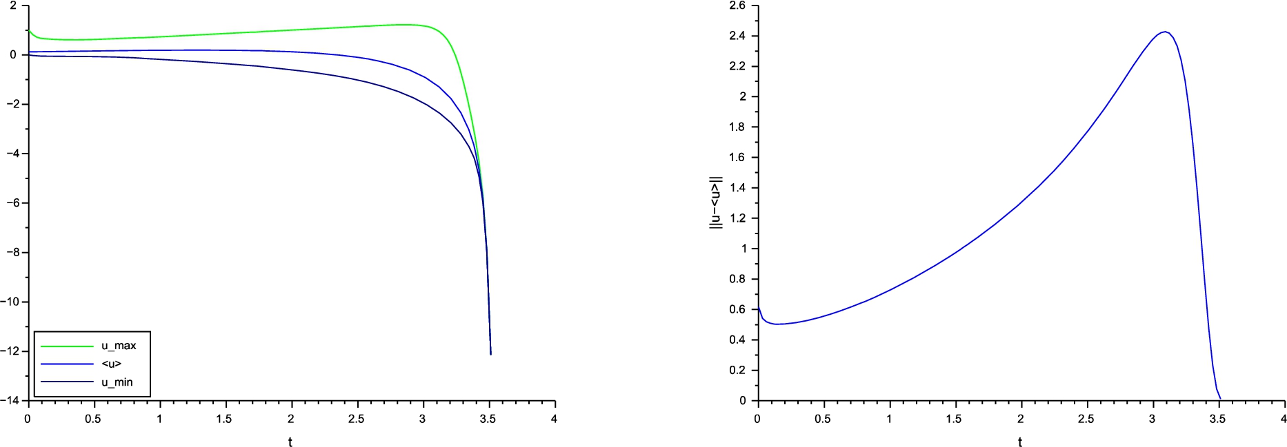
$u_{0} \in [0, 1]$ and $⟨ u_{0} ⟩ = 0.123$ , u blows up and $u - ⟨ u ⟩$ tends to 0.

In Fig. 1 , we take $g (s) = s^{2} - s$ , $u_{0} = 1 - {sin}^{2} (x + y)$ , and $H_{0} = 0$ , leading to $u_{0} \in [0, 1]$ and $⟨ u_{0} ⟩ = 0.424$ . In this case, u remains in the interval $[0, 1]$ for all $t ⩾ 0$ and converges to $\overline{u} \equiv 1$ .

Fig. 2 corresponds to the function $g (s) = s^{2} - s$ and the initial data $u_{0} = \frac{1}{(12 x^{6} + 1) (y^{5} + 1)}$ and $H_{0} = 0$ , resulting in $⟨ u_{0} ⟩ = 0.123$ . In this case, u blows up in finite time, while $‖ u - ⟨ u ⟩ ‖_{H^{2} (Ω)}$ converges to 0, in accordance with the theoretical results.

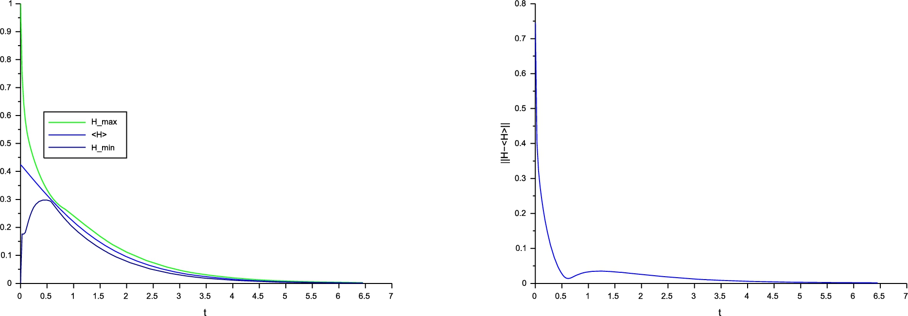
In Fig. 3 , we still take $g (s) = s^{2} - s$ with the initial data $u_{0} = {sin}^{2} (x + y)$ and $H_{0} = 1 - {sin}^{2} (x + y)$ , belonging to $[0, 1]$ , and $⟨ H_{0} ⟩ = 0.422$ . Here, H remains in the interval $[0, 1]$ for all $t ⩾ 0$ and converges to $\overline{H} = 0$ , confirming the theoretical results.

In Fig. 4 $, H$ blows up in finite time, while $‖ H - ⟨ H ⟩ ‖_{H^{1} (Ω)}$ converges to 0. Here, we take $g (s) = \frac{1}{2} s^{2} - s + \frac{1}{2}$ and the initial data $u_{0} = H_{0} = 1 - {sin}^{2} (x + y)$ , which leads to $⟨ H_{0} ⟩ = 0.486$ .

Fig. 3.

$H_{0} \in [0, 1]$ and $⟨ H_{0} ⟩ = 0.422$ , then H tends to 0.

Fig. 4.

$H_{0} \in [0, 1]$ and $⟨ H_{0} ⟩ = 0.486$ , H blows up and $H - ⟨ H ⟩$ tends to 0.

References

Aizicovici and

Feireisl, Long-time stabilization of solutions to a phase-field model with memory, Journal of Evolution Equations 1 (2001), 69–84. doi:10.1007/PL00001365.

Aizicovici,

Feireisl and

Issard-Roch, Long-time convergence of solutions to a phase-field system, Mathematical Methods in the Applied Sciences 24 (2001), 277–287. doi:10.1002/mma.215.

Boyer, Mathematical study of multi-phase flow under shear through order parameter formulation, Asymptot. Anal. 20 (1999), 175–212.

Brochet,

Chen and

Hilhorst, Finite dimensional exponential attractors for the phase-field model, Applied Analysis 49 (1993), 197–212.

Cagilnalp, Conserved-phase field system; implication for kinetic undercooling, Appl. Rev-B 38 (1988), 789–791. doi:10.1103/PhysRevB.38.789.

Caginalp, An analysis of a phase field model of a free boundary, Arch. Ration. Mech. Anal. 92 (1986), 205–245. doi:10.1007/BF00254827.

Caginalp and

Esenturk, Anisotropic phase field equations of arbitrary order, Discrete Contin. Dyn. Systems S 4 (2011), 311–350. doi:10.3934/dcdss.2011.4.311.

Cahn and

Hilliard, Free energy of a nonunifor system I. Interfacial free energy, J. Chem. Phys. 28 (1958), 258–267. doi:10.1063/1.1744102.

Cherfils,

Miranville and

Zelik, One a generalized Cahn–Hilliard equation with biological applications, disrete and continuous, Dynamical systems series B 19 (2014), 2013–2026.

10.

Cherfils,

Petcu and

Pierre, A numerical analysis of the Cahn–Hilliard equation with dynamic boundary conditions, Discrete Cont. Dyn. Systems 27 (2010), 1511–1533. doi:10.3934/dcds.2010.27.1511.

11.

Fakih, A Cahn–Hilliard equation with a proliferation term for biological and chemical applications, Asymptotic 94 (2015), 71–104. doi:10.3233/ASY-151306.

12.

FreeFem

+ +

is freely available at http://www.freefem.org/ff.

13.

Giacomin and

J.L.

Lebowitz, Phase segregation dynamics in particle systems with long range interaction I. Macroscopic limits, J. Statist. Phys. 87 (1997), 37–61. doi:10.1007/BF02181479.

14.

Giorgi,

Grasseli and

Pata, Uniform attractors for a phase-field model with memory and quadratic nonlinearity, Indiana Univ. Math. J 48 (1999), 1395–1446. doi:10.1512/iumj.1999.48.1793.

15.

Grasselli and

Pierre, A splitting method for the Cahn–Hilliard equation with inertial term, Math. Models Methods Appl. Sci. 20 (2010), 1363–1390. doi:10.1142/S0218202510004635.

16.

Gurtin,

Polignone and

Vinãls, Two-phase binary fluids and immiscible fluids described by an order parameter, Math. Models Methods Appli. Sci. 6 (1996), 815–831. doi:10.1142/S0218202596000341.

17.

Injrou and

Pierre, Stable discretizations of the Cahn–Hilliard–Gurtin equations, Discrete Cont. Dyn. Systems 22 (2008), 1065–1080. doi:10.3934/dcds.2008.22.1065.

18.

Nimi,

Langa et al., Robust exponential attractors for the Cahn–Hilliard–Oono–Navier–Stokes system, Discrete Cont. Dyn. Systems – Series S 9 (2023), 2426–2451.