The time horizon for stochastic homogenization of the one-dimensional wave equation

Abstract

The wave equation with stochastic rapidly oscillating coefficients can be classically homogenized on bounded time intervals; solutions converge in the homogenization limit to solutions of a wave equation with constant coefficients. This is no longer true on large time scales: Even in the periodic case with periodicity $ε$ , classical homogenization fails for times of the order $ε^{- 2}$ . We consider the one-dimensional wave equation with random rapidly oscillation coefficients on scale $ε$ and are interested in the critical time scale $ε^{- β}$ from where on classical homogenization fails. In the general setting, we derive upper and lower bounds for β in terms of the growth rate of correctors. In the specific setting of i.i.d. coefficients with matched impedance, we show that the critical time scale is $ε^{- 1}$ .

Keywords

Stochastic homogenization wave equation

1. Introduction

We are interested in homogenization limits for the wave equation with two x-dependent coefficients, the density ρ and the stiffness a. We focus on the case where these coefficients are random and consider, for a length scale parameter $ε > 0$ , the scaled functions $ρ_{ε} (x) := ρ (x / ε)$ and $a_{ε} (x) := a (x / ε)$ . The wave equation with unknown $u^{ε}$ then reads

\begin{aligned} ρ_{ε} \partial_{t}^{2} u^{ε} - \nabla \cdot (a_{ε} \nabla u^{ε}) = f_{ε}, \end{aligned}

(1.1)

where

f_{ε}

is given and the equation is completed with initial conditions for

u^{ε}

and

\partial_{t} u^{ε}

. The fundamental question of classical homogenization theory is to determine effective coefficients

\bar{ρ}

and

\bar{a}

such that solutions

u^{ε}

of (1.1) converge, in some appropriate sense, to a solution

\bar{u}

of the wave equation with the effective x-independent coefficients

\bar{ρ}

and

\bar{a}

In the setting of periodic homogenization, one assumes that ρ and a are periodic functions. Classical homogenization on bounded time intervals $[0, T_{0}]$ was investigated in [9]. It is worth mentioning that the homogenization of the wave equation is more involved than the homogenization of the corresponding parabolic problem; the difference is that the energy of high frequency contributions of solutions is not dissipated and may contribute error terms for the entire time of interest.

The seminal work [18] treated the question of larger time spans in periodic media. It was shown that a dispersive version of the wave equation must be considered in order to treat longer time spans. The effect was also clearly demonstrated in [13]. The first rigorous convergence result was given in [16] for one space dimension and in [10,11] for arbitrary space dimension. All these approaches show that dispersive effects are relevant on time intervals $[0, T_{0} ε^{- 2}]$ , for additional analysis see also [1,4], and, for the same effect in lattice equations, [20]. In particular, classical homogenization cannot hold on this time scale. In [3], the authors show that, in the periodic case, $ε^{- 2}$ is indeed the critical scale and classical homogenization holds on every scale $ε^{- 2 + δ}$ for $δ > 0$ . Regarding methods we would like to mention that Bloch Analysis was used in [10,11,18], while more direct energy methods are the basis of [1,3,16], and the later stochastic contributions. For general results regarding the two methods we mention [2].

Let us now turn to stochastic models, given by maps

\begin{aligned} ρ : R^{d} \times Ω_{P} \to [Λ^{- 1}, Λ] and a : R^{d} \times Ω_{P} \to [Λ^{- 1}, Λ] \end{aligned}

(1.2)

for some probability space

(Ω_{P}, A, P)

and some

Λ > 0

. We emphasize that positive upper and lower bounds for the coefficients are used. Suppressing, as usual, the stochastic parameter

ω \in Ω_{P}

, we write rescaled coefficients as

\begin{aligned} ρ_{ε} (x) := ρ (x / ε) = ρ (x / ε, ω) and a_{ε} (x) := a (x / ε) = a (x / ε, ω) . \end{aligned}

(1.3)

For the wave equation (1.1) with stochastic coefficients, there are several positive homogenization results available. In [7], convergence to the solution of a dispersive limit equation is shown in dimension $d ⩾ 4$ . It is even shown that arbitrary orders of convergence can be achieved by introducing a cascade of corrections in the equation in sufficiently large dimensions. This was recently put in a new perspective in [12]. For a quite general approach see [17]. For a detailed analysis of one-dimensional wave equations with stochastic coefficients on fixed time intervals we refer to [14]. The recently published book [8] gives an introduction to homogenization techniques; it covers various stochastic settings and provides examples of interesting effects even for one space dimension and for the stationary (elliptic) equation.

An important difference between random and periodic homogenization is the growth of correctors. In the periodic case, there exist bounded correctors to all orders, which is not true in a general random setting. Even under the best possible mixing assumptions, in general, there are only bounded correctors of order $d / 2$ (see, e.g., [7, Appendix C]). In particular, in the one-dimensional case, even the first order corrector is not bounded. The long-time homogenization results mentioned above rely either on periodic Bloch wave analysis or on expansions involving bounded higher order correctors. The fact that these correctors are only bounded if the dimension is sufficiently large leads to the dimensional restriction mentioned earlier. In particular, we are not aware of a stochastic homogenization result valid until the dispersive time-scale in dimension $d ⩽ 3$ .

In this contribution, we consider the one-dimensional case (where even first order correctors are unbounded). We are not concerned with possible dispersive limit equations, but rather with critical time scale for classical homogenization (non-dispersive constant coefficients limit model). We are interested in the following question for stochastic media:

For which parameters $β \in [0, 2]$ is the constant coefficient wave equation a good replacement for (1.1) on time intervals $[0, T_{0} ε^{- β}]$ ?

The critical number β will depend on the properties of the stochastic medium. In this contribution, we obtain two results related to this question: In the first result, we consider very general random media. These are characterised by a parameter $γ ⩾ 0$ , which is essentially the growth rate of correctors. We provide a lower critical value $β_{-} = β_{-} (γ) > 0$ and an upper critical value $β_{+} = β_{+} (γ) > 0$ with the following properties: For parameters $0 ⩽ β < β_{-}$ , homogenization with classical limits works on $[0, T_{0} ε^{- β}]$ for all models of class γ. For parameters $β > β_{+}$ , stochastic homogenization with classical limits is not valid for all models of class γ on time intervals $[0, T_{0} ε^{- β}]$ . The precise formulation of this result and the formulas for $β_{-} (γ)$ and $β_{+} (γ)$ are given in Theorem 2.6. Unfortunately, the two critical values do not coincide. The most standard stochastic medium (using i.i.d. coefficients) has the model parameter $γ = 1 / 2$ , the two critical parameters are $β_{-} = 1 / 3$ and $β_{+} = 1$ . In this sense, we have bounds for the critical time scale, but we cannot determine the exact value of the critical time scale at which stochastic homogenization fails. In our second main result, we consider the case of i.i.d. coefficients with matched impedance, i.e., $ρ a$ is a constant function. In this setting, we show that $ε^{- 1}$ (corresponding to $β = 1$ ) is the critical time-scale until which classical homogenization works, see Theorem 5.1.

To the best of our knowledge, we provide the first negative results on stochastic homogenization for the wave equation. The negative results in Theorem 2.6 and Theorem 5.1 rely on the same mechanism: the speed of wave packages in the random medium and in the corresponding (constant coefficient) homogenized equation is different on large time-scales. As mentioned above, we show that in the case of i.i.d. coefficients with matched impedance, homogenization works until that time-scale. This result relies on explicit formulas for solutions of the wave equations with matched impedance. In the general case, the situation is not clear and our analysis leaves open the following question: Consider the elementary i.i.d. stochastic medium with $γ = 1 / 2$ , $β_{-} = 1 / 3$ and $β_{+} = 1$ . What is the “real” critical value $β_{*} \in [1 / 3, 1]$ with the property that homogenization holds for $β < β_{*}$ and homogenization fails for $β > β_{*}$ ? We tried to find this value at least with numerical experiments, but we did not succeed to determine $β_{*} \in [1 / 3, 1]$ .

Our arguments for counter-examples are one-dimensional. We give some remarks on higher dimension in Section 2.4.

2. Notation and main result

2.1. Homogenized coefficients and correctors

In the one-dimensional case, the homogenized coefficients are given by simple formulas. Essentially, the effective density $\bar{ρ}$ is the arithmetic mean of ρ and the effective permeability $\bar{a}$ is the harmonic mean of a. Since we also consider non-ergodic media, we have a very general dependence on the spatial variable $x \in R^{n}$ ; this requires slightly more involved definitions. In any case, the stochastic setting allows to take expectations: In the probability space $(Ω_{P}, A, P)$ we denote the expected value of a random variable $f : Ω_{P} \to R$ with brackets $⟨ . ⟩$ and set $⟨ f ⟩ := \int_{Ω_{P}} f (ω) d P (ω)$ .

Since we do not impose stationarity or ergodicity of the medium, our definition of effective coefficients involves several averages. In one space dimension, we use the following concept.

Definition 2.1 (Effective coefficients in the sense of averages)

For $ρ, a : R \times Ω_{P} \to R$ , we define the effective coefficients in the sense of averages as

\begin{aligned} \bar{ρ} := lim_{| r | \to \infty} ⟨ - \int_{0}^{r} - \int_{0}^{y} ρ (s) d s d y ⟩, \bar{a} := lim_{| r | \to \infty} {⟨ - \int_{0}^{r} - \int_{0}^{y} 1 / a (s) d s d y ⟩}^{- 1}, \end{aligned}

(2.1)

demanding on the model functions ρ and a that the two limits of (2.1) exist. Note that we use a special sign convention for integrals, see (2.2) below.

In (2.1) and similar expressions in the subsequent text, we are interested in averages of the integrand. This means that, when we write $\int_{0}^{y} g (s) d s$ for negative y, we are indeed interested in the value of $\int_{[y, 0]} g (s) d s$ . In other words, we want that integrals of positive functions are positive, even when the limits of the integrand are not ordered in the usual way. We therefore set, for $y < 0$ ,

\begin{aligned} \int_{0}^{y} g (s) d s := \int_{y}^{0} g (s) d s and - \int_{0}^{y} g (s) d s := | y |^{- 1} \int_{y}^{0} g (s) d s . \end{aligned}

(2.2)

For periodic and, more generally, for stationary media, (2.1) can be replaced by simpler expressions. For stationary media, expectations are independent of y, hence $\bar{ρ} = ⟨ ρ (y, .) ⟩$ and $\bar{a} = ⟨ 1 / a (y, .) ⟩^{- 1}$ for arbitrary $y \in R$ . When the stochastic medium is ergodic, then spatial averages converge to expected values, hence, in this case, it is not necessary to take expectations in (2.1). For periodic media, the formula is even simpler: One can omit the expectation and integrate only over one periodicity cell.

In the one-dimensional setting, we can write the two wave equations of interest as follows. For coefficients ρ, a given by (1.2) and rescaled coefficients $ρ_{ε}$ , $a_{ε}$ given by (1.3) and a source $f : R \times R_{+} \to R$ , we consider the sequence of solutions $u^{ε} : R \times R_{+} \to R$ of the $ε$ -problem

\begin{aligned} ◻_{ε} u^{ε} := ρ_{ε} \partial_{t}^{2} u^{ε} - \partial_{x} (a_{ε} \partial_{x} u^{ε}) = f with u^{ε} (\cdot, 0) = \partial_{t} u^{ε} (\cdot, 0) = 0, \end{aligned}

(2.3)

and the solution

\bar{u} : R \times [0, \infty) \to R

of the limit problem

\begin{aligned} \bar{◻} \bar{u} := \bar{ρ} \partial_{t}^{2} \bar{u} - \partial_{x} (\bar{a} \partial_{x} \bar{u}) = f with \bar{u} (\cdot, 0) = \partial_{t} \bar{u} (\cdot, 0) = 0. \end{aligned}

(2.4)

We use here trivial initial data for notational convenience.

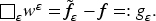
We turn to the construction of correctors and harmonic coordinates. The one-dimensional corrector equation reads $\partial_{y} [a (y) (1 + \partial_{y} Φ (y))] = 0$ for $y \in R$ . For a given coefficient field a, one seeks a solution $Φ : R \to R$ of this equation. In one space dimension, the solution is given by an integral: Since the argument in the squared brackets must be independent of y, the squared bracket coincides with some constant. The constant value is indeed the effective coefficient, $a (y) (1 + \partial_{y} Φ (y)) = \bar{a}$ for every $y \in R$ . Dividing by $a (y)$ and integrating over y, this formula can be used to define Φ. The procedure for the corrector $Ψ$ for ρ is similar.

Definition 2.2 (Correctors)

Let $ρ, a : R \times Ω_{P} \to (0, \infty)$ be stochastic coefficients and let $\bar{ρ}$ and $\bar{a}$ be two positive numbers. We define corresponding correctors as

\begin{aligned} Ψ (y) := Ψ (y, ω) := \int_{0}^{y} {\frac{ρ (s)}{\bar{ρ}} - 1} d s, Φ (y) := Φ (y, ω) := \int_{0}^{y} {\frac{\bar{a}}{a (s)} - 1} d s, \end{aligned}

(2.5)

where we suppressed the argument ω also in ρ and a.

Dependence on coefficients. We note that the correctors depend on the coefficients ρ and a and on the effective coefficients $\bar{ρ}$ and $\bar{a}$ . Indeed, one can regard $\bar{ρ}$ and $\bar{a}$ as being chosen in such a way that the correctors have minimal growth.

Rescaling. Rescaled coefficients are defined by $ρ_{ε} (x) = ρ (x / ε)$ and $a_{ε} (x) = a (x / ε)$ . The correctors are rescaled as $Φ_{ε} (x) := ε Φ (x / ε)$ and $Ψ_{ε} (x) := ε Ψ (x / ε)$ . We note that $Φ_{ε}$ satisfies, for every $x \in R$ ,

\begin{aligned} \begin{matrix} \partial_{x} [(a_{ε} (x) (1 + \partial_{x} Φ_{ε} (x))] = 0, \end{matrix} \end{aligned}

and

\begin{aligned} a_{ε} (x) (1 + \partial_{x} Φ_{ε} (x)) = \bar{a} . \end{aligned}

(2.6)

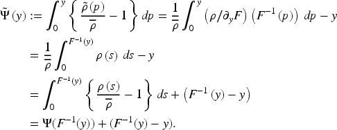
Harmonic coordinates. Related to the correctors are harmonic coordinates. Later on we use the function

F (y) := y + Φ (y)

to perform a change of coordinates that simplifies the equation. The rescaling for the function F is given by

F_{ε} (x) := ε F (x / ε) = x + Φ_{ε} (x)

In this article, we study the question whether or not the homogenized solution $\bar{u}$ is a good approximation for the heterogeneous media solution $u^{ε}$ . The answer depends on the time span of interest and on the “quality” of the stochastic medium. We will measure the latter in terms of growth rates of the correctors.

2.2. Model classes and first main result

Let $(Ω_{P}, A, P)$ be a probability space, let ρ and a be stochastic coefficients, and let the space dimension be $d = 1$ .

Definition 2.3 (Model class parameter γ)

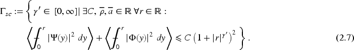
For fixed $Λ ⩾ 1$ we consider maps $ρ, a : R \times Ω_{P} \to [\frac{1}{Λ}, Λ]$ . Given ρ and a and two positive numbers $\bar{ρ}$ and $\bar{a}$ , we denote the corresponding correctors as $Ψ$ and Φ, see Definition 2.2. We define the set of supercritical parameters $γ^{'}$ as

\begin{aligned} Γ_{s c} := & {γ^{'} \in [0, \infty] | \exists C, \bar{ρ}, \bar{a} \in R \forall r \in R : \\ ⟨ - \int_{0}^{r} {| Ψ (y) |}^{2} d y ⟩ + ⟨ - \int_{0}^{r} {| Φ (y) |}^{2} d y ⟩ ⩽ C {(1 + | r |^{γ^{'}})}^{2}} . \end{aligned}

(2.7)

The model class parameter γ is set to be

\begin{aligned} γ := inf Γ_{s c} . \end{aligned}

(2.8)

With this definition, we associate to a model (given by random fields a and ρ) a model class parameter

γ = γ (ρ, a)

Remarks. 1.) The class is a number $γ \in [0, 1]$ . We recall that we always assume boundedness of a and ρ. Under this assumption, the functions Φ and $Ψ$ have at most linear growth, which implies $(1, \infty) \subset Γ_{s c}$ and hence $γ ⩽ 1$ . By definition, there always holds $γ ⩾ 0$ .

2.) Interpretation and periodic media. With $γ \in [0, 1]$ defined as above, we say that $(ρ, a)$ defines a model of class γ. The quantity γ quantifies the sublinearity of the correctors. We recall the periodic coefficients have bounded correctors, hence the model parameter for periodic coefficients is $γ = 0$ .

3.) Effective coefficients in the sense of optimal correctors. The definition can also be used to define effective coefficients: The numbers $\bar{ρ}$ and $\bar{a}$ for which the optimal growth rate in (2.7) is obtained are the effective coefficients in the sense of optimal correctors.

We emphasize that the two possible definitions of effective coefficients are closely related. We will show in Lemma 4.4 the following: When the growth of (2.7) holds for $\bar{ρ}$ and $\bar{a}$ and for a number $γ^{'} < 1$ , then $\bar{ρ}$ and $\bar{a}$ are the effective coefficients in the sense of averages of Definition 2.1.

Example 2.4 (The simplest stochastic medium)

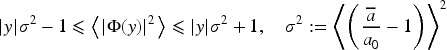
Let $(a_{j})_{j \in Z}$ and $(ρ_{j})_{j \in Z}$ be i.i.d. random variables, chosen with a uniform distribution in $[1, 2]$ . We define a and ρ by setting $a (x) = a_{j}$ and $ρ (x) = ρ_{j}$ for $x \in [j, j + 1)$ , and we set $\bar{ρ} = ⟨ ρ_{0} ⟩$ and $\bar{a} := ⟨ a_{0}^{- 1} ⟩^{- 1}$ . This defines a stochastic model. The model class parameter of this model is $γ = 1 / 2$ .

Let us sketch how to calculate the model parameter γ. For large $y \in N$ , the quantities $Φ (y)$ and $Ψ (y)$ of (2.5) are sums of y i.i.d. random variables with vanishing expected value, in particular we have for $Φ (y)$ , with $y \in R$ ,

\begin{aligned} | y | σ^{2} - 1 ⩽ ⟨ {| Φ (y) |}^{2} ⟩ ⩽ | y | σ^{2} + 1, σ^{2} := {⟨ (\frac{\bar{a}}{a_{0}} - 1) ⟩}^{2} \end{aligned}

(for

Ψ (y)

holds an analogous estimate with

σ^{2} := ⟨ (\frac{ρ_{0}}{\bar{ρ}} - 1)^{2} ⟩

). We conclude that the expressions in (2.7) behave like (we write the formulas for Φ and

y > 0

\begin{aligned} \frac{σ^{2}}{2} y - 1 = - \int_{0}^{y} σ^{2} s - 1 d s ⩽ ⟨ - \int_{0}^{y} {| Φ (s) |}^{2} d s ⟩ ⩽ - \int_{0}^{y} σ^{2} s + 1 d s = \frac{σ^{2}}{2} y + 1. \end{aligned}

The above estimate, together with the analogous estimate for

Ψ

, yield

γ = 1 / 2

For media with growth parameter $γ \in (1 / 2, 1)$ , we refer to Appendix C.

We have to make precise what we mean with the sloppy expression “homogenization works”. The subsequent gives a definition. On the one hand, we have to introduce the parameter β that measures the time span under consideration. On the other hand, we have to choose a notion of convergence. Regarding the latter, it seems natural to work with the norms that are suggested by energy estimates, i.e., we use an $L^{\infty}$ -norm in time, and measure first derivatives with the norm $L^{2}$ in the spatial coordinate. We actually leave out first spatial derivatives, since one expects oscillations of $\partial_{x} u^{ε}$ , but no oscillations of $\partial_{x} \bar{u}$ . To compare only time derivatives turns out to be the more robust concept.

Definition 2.5 (Homogenization time parameter β)

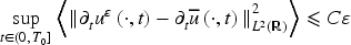
Let $ρ, a : R \times Ω_{P} \to R$ be stochastic coefficients and let $β \in [0, \infty)$ be a positive parameter. We say that classical homogenization works with parameter β if the following holds: For any $f \in C^{2} (R \times R_{+}, R)$ with compact support and any $T_{0} > 0$ , the solutions $u^{ε}$ of (2.3) and $\bar{u}$ of (2.4) satisfy

\begin{aligned} lim_{ε \to 0} sup_{t \in [0, T_{0} ε^{- β}]} ⟨ {‖ \partial_{t} u^{ε} (\cdot, t) - \partial_{t} \bar{u} (\cdot, t) ‖}_{L^{2} (R)} ⟩ = 0. \end{aligned}

(2.9)

Loosely speaking: $β ⩾ 0$ is the parameter such that classical stochastic homogenization works on time intervals $[0, T_{0} ε^{- β}]$ .

We can now formulate our first main result.

Theorem 2.6 Critical parameters

Let $γ \in [0, 1]$ be a number such that a model of that class exists. With the critical parameters

\begin{aligned} β_{-} := \frac{1 - γ}{1 + γ}, β_{+} := \frac{1 - γ}{γ} \end{aligned}

(2.10)

there holds:

(1)

For $β \in [0, β_{-})$ : For all coefficients $(ρ, a)$ of class γ, classical homogenization works with parameter β.

(2)

For $β \in (β_{+}, \infty)$ : There exist coefficients $(ρ, a)$ of class γ such that classical homogenization does not work with parameter β.

The main novelty of Theorem 2.6 is Part (2), while Part (1) follows by well established computations.

Remark 2.7 (The class of models with i.i.d. coefficients)

We described the case of i.i.d. coefficients in Example 2.4 and noted that it corresponds to $γ = 1 / 2$ . In this case, we have $β_{-} = (1 / 2) / (3 / 2) = 1 / 3$ and $β_{+} = 1$ . Accordingly, Theorem 2.6 implies that, for all $β \in [0, 1 / 3)$ , classical homogenization is valid. This matches previous findings, e.g. [12, Theorem 3 and Eq. (1.13)].

We emphasize that Part (2) of Theorem 2.6 does not imply that there exists i.i.d. coefficients such that for $β > 1$ homogenization fails. It only ensures that there exist a model of class $γ = 1 / 2$ such that homogenization fails.

However, as mentioned above, Theorem 5.1 provides a sharp threshold for i.i.d. coefficients with matched impedance, $a_{i} ρ_{i} = 1$ for all $i \in Z^{d}$ . The threshold is $β = β_{+} = 1$ .

Section 3 is devoted to the first claim of the theorem, the positive homogenization result. Section 4 is devoted to the second claim of the theorem, the negative result.

2.3. The case of matched impedance

The main novelty of Theorem 2.6 is Part (2), which concerns the failure of classical homogenization on sufficiently large time spans. In the special class of media with matched impedance one can understand well the mechanism of this failure. It is related to a large likelihood of a wrong averaged wave speed on a considerable time span. We would like to mention that we learned the techniques for matched impedance media from [14]. Below we provide an informal (but detailed) discussion of the failure of homogenization in media with matched impedance; rigorous results in this setting can be found in Section 5.

A medium has matched impedance if the product $ρ \cdot a$ is a constant function. Here, we assume that $ρ (x, ω) \cdot a (x, ω) = 1$ holds for all $x \in R$ and for $P$ -almost every $ω \in Ω_{P}$ .

In this section, we sketch the idea leading to negative results on homogenization in the case of matched impedance. For precise statements and rigorous proofs, we refer to Theorem 5.1 in Section 5. In addition, we provide in Theorem 5.1 a positive homogenization results which is significantly stronger than Part (1) of Theorem 2.6.

A stochastic medium with matched impedance. We consider coefficients $a = a (x)$ that are piecewise constant in the intervals, $a (x) = a_{j}$ for every $x \in [j, j + 1) =: I_{j}$ . The numbers $a_{j} \in [Λ^{- 1}, Λ]$ are chosen as i.i.d. random variables. A possible choice is to pick $a_{j}$ according to a uniform distribution on the interval $[1, 2]$ . We set $ρ_{j} = 1 / a_{j}$ for every j and $ρ (x) := ρ_{j}$ for all $x \in I_{j}$ . This construction guarantees a constant impedance, $ρ \cdot a = 1$ on $R$ .

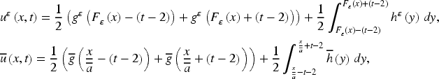
Solutions of the wave equation. In this setting, there is an explicit formula for solutions. Let $g : R \to R$ of class $C^{2}$ be an arbitrary function with compact support in $R_{+}$ . We define a function u as follows: For every $x > 0$ and $t ⩾ 0$ , we set

\begin{aligned} u (x, t) := g (\frac{x - j}{a_{j}} - t + \sum_{i = 0}^{j - 1} \frac{1}{a_{i}}) for x \in I_{j}, \end{aligned}

(2.11)

using the convention that empty sums are zero,

\sum_{i = 0}^{- 1} = 0

. We extend trivially by setting

u (x, t) = 0

for

x < 0

. We claim that u solves the wave equation.

Before we verify the claim, let us calculate the initial values of u. For $x < 0$ , there holds $u (x, 0) = 0$ . For $0 ⩽ x \in I_{j}$ , there holds $x = j + h$ for some $h \in [0, 1)$ and $u (x, 0) = g (h / a_{j} + \sum_{i = 0}^{j - 1} (1 / a_{i}))$ . In particular, g does not coincide with the initial values of u.

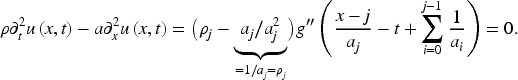
Let us now show that, independent of initial data, u solves the wave equation. In the interior of the interval $I_{j}$ , we can calculate classically

\begin{aligned} ρ \partial_{t}^{2} u (x, t) - a \partial_{x}^{2} u (x, t) = (ρ_{j} - \underset{= 1 / a_{j} = ρ_{j}}{\underset{⏟}{a_{j} / a_{j}^{2}}}) g^{″} (\frac{x - j}{a_{j}} - t + \sum_{i = 0}^{j - 1} \frac{1}{a_{i}}) = 0. \end{aligned}

It remains to show continuity of u and of the fluxes

a \partial_{x} u

at the interfaces, i.e., at

x = j \in Z

. Regarding continuity of u we calculate

\begin{aligned} \begin{matrix} lim_{x ↗ j} u (x, t) = g (\frac{j - (j - 1)}{a_{j - 1}} - t + \sum_{i = 0}^{j - 2} \frac{1}{a_{i}}) = g (\frac{1}{a_{j - 1}} - t + \sum_{i = 0}^{j - 2} \frac{1}{a_{i}}) = lim_{x ↘ j} u (x, t) . \end{matrix} \end{aligned}

We now verify the continuity of fluxes at

x = j \in Z

\begin{aligned} lim_{x ↗ j} a (x) \partial_{x} u (x, t) = g^{'} (\frac{1}{a_{j - 1}} - t + \sum_{i = 0}^{j - 2} \frac{1}{a_{i}}) = lim_{x ↘ j} a (x) \partial_{x} u (x, t), \end{aligned}

where we exploited

a_{j - 1} / a_{j - 1} = 1 = a_{j} / a_{j}

. We have verified that u is a solution of the wave equation with coefficients a and ρ (see Appendix A for a integral representation of solutions of the Cauchy–Problem in the case of matched impedance).

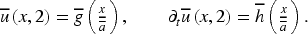
Homogenization. Let us now consider the rescaled coefficients $a_{ε} = a (\cdot / ε)$ and $ρ_{ε} = ρ (\cdot / ε)$ . A solution $u^{ε}$ of the wave equation is given by formula (2.11), which is modified to

\begin{aligned} u^{ε} (x, t) = g (\frac{x - ε j}{a_{j}} - t + \sum_{i = 0}^{j - 1} \frac{ε}{a_{i}}) for x \in [ε j, ε (j + 1)) . \end{aligned}

(2.12)

We note that one can also express j in terms of x as

j = ⌊ x / ε ⌋

in order to have a single formula for all

x > 0

The effective parameter $\bar{a}$ is the harmonic average of $a_{j}$ , with our choices it is given by a simple expectation, ${\bar{a}}^{- 1} = ⟨ 1 / a_{j} ⟩$ for any $j \in Z$ . The effective parameter $\bar{ρ}$ is the arithmetic average of $ρ_{j}$ , in our setting $\bar{ρ} = ⟨ ρ_{j} ⟩ = ⟨ 1 / a_{j} ⟩ = {\bar{a}}^{- 1}$ . We see that the impedance of the effective medium is again 1 and that the effective speed is $\bar{c} = \bar{a}$ . The effective wave equation is

\begin{aligned} \frac{1}{\bar{a}} \partial_{t}^{2} \bar{u} - \bar{a} \partial_{x}^{2} \bar{u} = 0. \end{aligned}

(2.13)

A solution to this equation is given, for

x > 0

, by

\begin{aligned} \bar{u} (x, t) = g (\frac{x}{\bar{a}} - t) . \end{aligned}

(2.14)

We claim that stochastic homogenization fails in this setting on time intervals $[0, T_{0} ε^{- β}]$ when we choose $β > 1$ . To see this, it suffices to compare $u^{ε}$ of (2.12) and $\bar{u}$ of (2.14). This is sufficient since, for t in bounded time intervals, there holds $u^{ε} \approx \bar{u}$ for small $ε > 0$ (and recall that rigorous results are presented in Section 5).

Calculating the difference. Let us assume that the support of g is contained in $[0, 2]$ , that the maximal value of g is 1 and that this maximum is attained in the point $x = 1$ . The solution $\bar{u}$ is a shift of the initial values, in this sense it is a wave that travels with speed $\bar{a}$ to the right. For every observation point $x > 1$ , the peak of the wave arrives at the time $\bar{T} (x)$ at which the argument of g in (2.14) is 1, i.e., $\bar{T} (x) := - 1 + (x / \bar{a})$ . In more mathematical terms: For $x > 1$ , the function $\bar{u} (x, .) : [0, \infty) \to R$ has its maximum at $t = \bar{T} (x)$ , the value in this maximum is 1.

We want to calculate the time instance ${\bar{T}}_{ε} (x)$ at which the function $u^{ε} (x, .) : [0, \infty) \to R$ is maximal. The maximum of $u^{ε} (x, .)$ is at the point ${\bar{T}}_{ε} (x)$ for which the argument of g in (2.12) is 1, hence

\begin{aligned} {\bar{T}}_{ε} (x) = \frac{x - j ε}{a_{j}} - 1 + \sum_{i = 0}^{j - 1} \frac{ε}{a_{i}}, \end{aligned}

(2.15)

where j is such that

x \in [ε j, ε (j + 1))

holds, that is,

j = ⌊ x / ε ⌋

We are interested in the mismatch of the arrival times for the $ε$ -solution and the homogenized solution,

\begin{aligned} Δ_{ε} (x) := {\bar{T}}_{ε} (x) - \bar{T} (x) = \frac{x - ε ⌊ x / ε ⌋}{a_{j}} + \sum_{i = 0}^{j - 1} \frac{ε}{a_{i}} - \frac{x}{\bar{a}} . \end{aligned}

(2.16)

Let us consider a fixed grid point

x = ε j

. At this point, the expected value of the mismatch is

\begin{aligned} ⟨ Δ_{ε} (x) ⟩ = ⟨ - \frac{x}{\bar{a}} + \sum_{i = 0}^{j - 1} \frac{ε}{a_{i}} ⟩ = ε j (\frac{1}{\bar{a}} - ⟨ \frac{1}{a_{i}} ⟩) = 0. \end{aligned}

(2.17)

This agrees with intuition, we expect that the wave arrives at the time that is suggested by the homogenized equation.

For our analysis, it is not sufficient to calculate the averaged arrival time. Homogenization fails when, with a positive probability, we observe a wrong arrival time in the stochastic medium. Let us therefore calculate the typical size of the random variable $Δ_{ε} (x)$ . For the calculation we use the quantity $σ ⩾ 0$ , defined by the expectation $σ^{2} := ⟨ | (1 / a_{i}) - (1 / \bar{a}) |^{2} ⟩$ for any i. The number $σ > 0$ is the variance of the single entry in the sum. The independence of the random variables $a_{i}$ allows to calculate, again for $x = ε j$ ,

\begin{aligned} ⟨ | Δ_{ε} (x) |^{2} ⟩ & = ⟨ {| \frac{ε j}{\bar{a}} - \sum_{i = 0}^{j - 1} \frac{ε}{a_{i}} |}^{2} ⟩ = ε^{2} ⟨ {| \sum_{i = 0}^{j - 1} \frac{1}{\bar{a}} - \frac{1}{a_{i}} |}^{2} ⟩ \\ = ε^{2} ⟨ \sum_{i = 0}^{j - 1} {| \frac{1}{\bar{a}} - \frac{1}{a_{i}} |}^{2} ⟩ = ε^{2} j σ^{2} . \end{aligned}

(2.18)

For

β ⩾ 0

and

ε \in (0, \frac{1}{4}]

, we consider

j_{ε} = ⌊ ε^{- 1 - β} ⌋

and

x_{ε} = ε j_{ε}

. Clearly, we have

| x_{ε} | ⩽ 2 ε^{- β}

j_{ε} ⩾ \frac{1}{2} ε^{- 1 - β}

, and the arrival times of the pulse

u^{ε}

and the pulse

\bar{u}

typically differ by the order

\begin{aligned} | {\bar{T}}_{ε} (x_{ε}) - \bar{T} (x_{ε}) | = | Δ_{ε} (x_{ε}) | = O (\sqrt{ε^{2} j_{ε} σ^{2}}) ⩾ O (σ \sqrt{ε^{1 - β}}) . \end{aligned}

(2.19)

For

β ⩾ 1

, this deviation is not small. We therefore expect that, typically, the two waves arrive at x with an order 1 mismatch, which leads also to an order 1 mismatch between the two solutions of the wave equation. The calculation strongly suggests that homogenization fails on the time scale

ε^{- β}

for

β ⩾ 1

. Note that, in the above discussion,

u^{ε}

and

\bar{u}

(see (2.12) and (2.13)) do not satisfy the same initial conditions. We recall that rigorous result – positive and negative – are given in Section 5.

2.4. Remarks on higher dimensions

In Theorem 2.6, we provide two critical parameters, $β_{-}$ and $β_{+}$ . The lower critical parameter, $β_{-} = β_{-} (γ) = (1 - γ) / (1 + γ)$ , is related to positive homogenization results. It is derived in Section 3. The techniques of that section are well-established and independent of the dimension. It is possible to define a growth rate of correctors also in higher dimensions and to derive, with similar methods as in Section 3, positive homogenization results until time-scales $ε^{- β_{-}}$ , where $β_{-}$ depends on the growth rate. We mentioned that recent advances in quantitative stochastic homogenization yield optimal estimates on the growth of the correctors for large classes of random media, see e.g. [5,15] and the references therein.

The upper critical parameter $β_{+} = β_{+} (γ) = (1 - γ) / γ$ is based on the construction of counter-examples. The counter-examples use either media with matched impedance or media-adapted domain transformations. In any case: If one considers layered media in dimension $d > 1$ , then the one-dimensional counter-examples still provide examples where homogenization does not hold. We mention that a restriction to initial values with compact support would still require some work, but we would not expect severe difficulties to the construction of counter-examples.

On the other hand, for stochastic media that exploit the full liberty of media in higher dimension, we do not have any counter-examples and they cannot be constructed easily following the ideas that are used in this contribution.

3. The lower critical parameter

In this section we derive estimates for the homogenization error and prove Part (1) of Theorem 2.6: $u^{ε} \approx \bar{u}$ when t is not too large.

Following a standard approach, we first compare the solution $u^{ε}$ of (2.3) with the two-scale expansion $\bar{u} + Φ_{ε} \partial_{x} \bar{u}$ of the solution $\bar{u}$ of (2.4). This comparison is the aim of the subsequent lemma.

Lemma 3.1 Energy estimate for the error

Let $(ρ, a)$ be a model of class $γ \in [0, 1)$ with bounds given by $Λ > 0$ . Then, for every $γ^{'} > γ$ and every $M ⩾ 1$ , there exists $C = C (Λ, γ^{'}, M) > 0$ such that the following is true: Let $f \in C^{2} (R \times R_{+})$ be supported in $[- M, M] \times [0, M]$ , for $ε \in (0, 1]$ let $u^{ε}$ and $\bar{u}$ be the unique solutions to (2.3) and (2.4), respectively, and let $z_{ε}$ be defined as

\begin{aligned} z_{ε} := u^{ε} - (\bar{u} + Φ_{ε} \partial_{x} \bar{u}) . \end{aligned}

(3.1)

For every

T ⩾ 1

holds

\begin{aligned} sup_{t \in [0, T]} ⟨ E_{ε} (t) ⟩ ⩽ C ε^{2 (1 - γ^{'})} T^{2 (1 + γ^{'})} ‖ f ‖_{C^{2} (R \times R_{+})}^{2}, \end{aligned}

(3.2)

where

\begin{aligned} E_{ε} (t) := \frac{1}{2} \int_{R} ρ_{ε} {| \partial_{t} z_{ε} (x, t) |}^{2} + a_{ε} {| \partial_{x} z_{ε} (x, t) |}^{2} d x . \end{aligned}

(3.3)

Proof.

The following argument closely follows [19, Lemma 3.3]. Clearly, it suffices to prove the claim for $M = 1$ . We therefore fix $f \in C^{2} (R \times R_{+})$ with support in $[- 1, 1] \times [0, 1]$ .

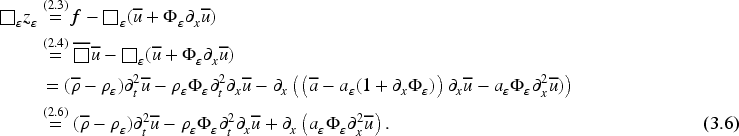
Step 1: Equation for $z_{ε}$ . We claim that $z_{ε}$ of (3.1) satisfies

\begin{aligned} ◻_{ε} z_{ε} = ρ_{ε} g_{ε}^{(1)} + \partial_{x} (a_{ε} g_{ε}^{(2)}), \end{aligned}

(3.4)

where

◻_{ε}

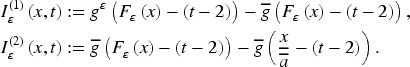
is defined in (2.3) and the error functions are

\begin{aligned} g_{ε}^{(1)} := - (Φ_{ε} - (\bar{ρ} / ρ_{ε}) Ψ_{ε}) \partial_{t}^{2} \partial_{x} \bar{u}, g_{ε}^{(2)} := Φ_{ε} \partial_{x}^{2} \bar{u} - (\bar{ρ} / a_{ε}) Ψ_{ε} \partial_{t}^{2} \bar{u} . \end{aligned}

(3.5)

With the help of (2.3), (2.4) and (2.6) we compute

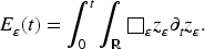
\begin{aligned} ◻_{ε} z_{ε} & \overset{(2.3)}{=} f - ◻_{ε} (\bar{u} + Φ_{ε} \partial_{x} \bar{u}) \\ \overset{(2.4)}{=} \bar{◻} \bar{u} - ◻_{ε} (\bar{u} + Φ_{ε} \partial_{x} \bar{u}) \\ = (\bar{ρ} - ρ_{ε}) \partial_{t}^{2} \bar{u} - ρ_{ε} Φ_{ε} \partial_{t}^{2} \partial_{x} \bar{u} - \partial_{x} ((\bar{a} - a_{ε} (1 + \partial_{x} Φ_{ε})) \partial_{x} \bar{u} - a_{ε} Φ_{ε} \partial_{x}^{2} \bar{u})) \\ \overset{(2.6)}{=} (\bar{ρ} - ρ_{ε}) \partial_{t}^{2} \bar{u} - ρ_{ε} Φ_{ε} \partial_{t}^{2} \partial_{x} \bar{u} + \partial_{x} (a_{ε} Φ_{ε} \partial_{x}^{2} \bar{u}) . \end{aligned}

(3.6)

The first term on the right-hand side in (3.6) can be expressed with the help of

Ψ_{ε}

, defined in (2.5):

\begin{aligned} (\bar{ρ} - ρ_{ε}) \partial_{t}^{2} \bar{u} = - (\bar{ρ} \partial_{x} Ψ_{ε}) \partial_{t}^{2} \bar{u} = - \bar{ρ} \partial_{x} (Ψ_{ε} \partial_{t}^{2} \bar{u}) + \bar{ρ} Ψ_{ε} \partial_{x} \partial_{t}^{2} \bar{u} . \end{aligned}

The claimed identity (3.4) follows.

Step 2: Energy estimate. We claim that

\begin{aligned} sup_{t \in [0, T]} ⟨ E_{ε} (t) ⟩ & ⩽ T Λ \int_{0}^{T} ⟨ {‖ g_{ε}^{(1)} (\cdot, s) ‖}_{L^{2} (R))}^{2} ⟩ + ⟨ {‖ \partial_{t} g_{ε}^{(2)} (\cdot, s) ‖}_{L^{2} (R))}^{2} ⟩ d s \\ + 8 Λ sup_{t \in [0, T]} ⟨ {‖ g_{ε}^{(2)} (\cdot, t) ‖}_{L^{2} (R))}^{2} ⟩ . \end{aligned}

(3.7)

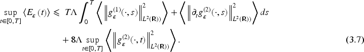
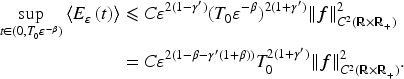
The derivation of (3.7) follows with a standard procedure of the theory of the linear wave equation: We multiply (3.4) with $\partial_{t} z_{ε}$ and integrate, for arbitrary $t \in [0, T]$ , over $R \times (0, t)$ . Since $z_{ε}$ satisfies homogeneous initial conditions, an integration by parts allows to write the energy expression of (3.3) in the form

\begin{aligned} E_{ε} (t) & = \int_{0}^{t} \int_{R} ◻_{ε} z_{ε} \partial_{t} z_{ε} . \end{aligned}

Equation (3.4) therefore yields, using again

z_{ε} (\cdot, 0) = 0

\begin{aligned} E_{ε} (t) & = \int_{0}^{t} \int_{R} [ρ_{ε} g_{ε}^{(1)} + \partial_{x} (a_{ε} g_{ε}^{(2)})] \partial_{t} z_{ε} \\ = \int_{0}^{t} \int_{R} {ρ_{ε} g_{ε}^{(1)} \partial_{t} z_{ε} + a_{ε} \partial_{t} g_{ε}^{(2)} \partial_{x} z_{ε}} - \int_{R} a_{ε} (x) g_{ε}^{(2)} (x, t) \partial_{x} z_{ε} (x, t) d x . \end{aligned}

(3.8)

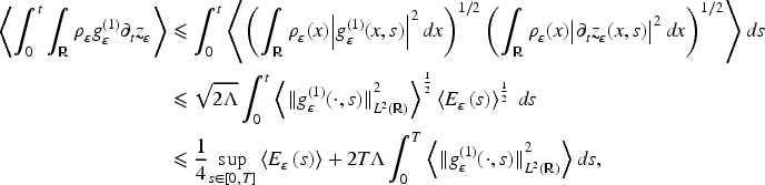
Taking expectations and using

ρ_{ε} ⩽ Λ

, we estimate the first term on the right hand side, for arbitrary

t \in [0, T]

\begin{aligned} ⟨ \int_{0}^{t} \int_{R} ρ_{ε} g_{ε}^{(1)} \partial_{t} z_{ε} ⟩ & ⩽ \int_{0}^{t} ⟨ {(\int_{R} ρ_{ε} (x) {| g_{ε}^{(1)} (x, s) |}^{2} d x)}^{1 / 2} {(\int_{R} ρ_{ε} (x) {| \partial_{t} z_{ε} (x, s) |}^{2} d x)}^{1 / 2} ⟩ d s \\ ⩽ \sqrt{2 Λ} \int_{0}^{t} {⟨ {‖ g_{ε}^{(1)} (\cdot, s) ‖}_{L^{2} (R)}^{2} ⟩}^{\frac{1}{2}} {⟨ E_{ε} (s) ⟩}^{\frac{1}{2}} d s \\ ⩽ \frac{1}{4} sup_{s \in [0, T]} ⟨ E_{ε} (s) ⟩ + 2 T Λ \int_{0}^{T} ⟨ {‖ g_{ε}^{(1)} (\cdot, s) ‖}_{L^{2} (R)}^{2} ⟩ d s, \end{aligned}

where we use Young’s inequality in the last inequality. A similar calculation allows to estimate the expectation of the second term on the right hand side of (3.8):

\begin{aligned} ⟨ \int_{0}^{t} \int_{R} a_{ε} \partial_{t} g_{ε}^{(2)} \partial_{x} z_{ε} ⟩ ⩽ \frac{1}{4} sup_{s \in [0, T]} ⟨ E_{ε} (s) ⟩ + 2 T Λ \int_{0}^{T} ⟨ {‖ \partial_{t} g_{ε}^{(2)} (\cdot, s) ‖}_{L^{2} (R)}^{2} ⟩ d s . \end{aligned}

Regarding the last term in (3.8), we find, for every

t \in [0, T]

\begin{aligned} ⟨ \int_{R} | a_{ε} g_{ε}^{(2)} (x, t) \partial_{x} z_{ε} (x, t) | d x ⟩ ⩽ \frac{1}{4} sup_{s \in [0, T]} ⟨ E_{ε} (s) ⟩ + 2 Λ sup_{s \in [0, T]} ⟨ {‖ g_{ε}^{(2)} (\cdot, s) ‖}_{L^{2} (R)}^{2} ⟩ . \end{aligned}

Combining the last three displayed formulas with (3.8), we obtain (3.7).

Step 3: Estimating $g_{ε}^{(1)}$ and $g_{ε}^{(2)}$ . The solution $\bar{u}$ of (2.4) can be expressed by the following d’Alembert type representation formula with $c = \sqrt{\bar{a} / \bar{ρ}}$ :

\begin{aligned} \bar{u} (x, t) = \frac{1}{2 \bar{ρ}} \int_{0}^{t} \int_{x - c (t - s)}^{x + c (t - s)} f (y, s) d y d s . \end{aligned}

(3.9)

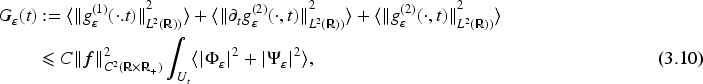
This representation of

\bar{u}

allows to estimate the error functions. We claim that there exists

C = C (Λ) \in [1, \infty)

such that, for every

t \in [0, T]

\begin{aligned} G_{ε} (t) & := ⟨ {‖ g_{ε}^{(1)} (\cdot . t) ‖}_{L^{2} (R))}^{2} ⟩ + ⟨ {‖ \partial_{t} g_{ε}^{(2)} (\cdot, t) ‖}_{L^{2} (R))}^{2} ⟩ + ⟨ {‖ g_{ε}^{(2)} (\cdot, t) ‖}_{L^{2} (R))}^{2} ⟩ \\ ⩽ C ‖ f ‖_{C^{2} (R \times R_{+})}^{2} \int_{U_{t}} ⟨ | Φ_{ε} |^{2} + | Ψ_{ε} |^{2} ⟩, \end{aligned}

(3.10)

where the domain of integration is, with

c = \sqrt{\bar{a} / \bar{ρ}}

as above,

\begin{aligned} U_{t} := [- c t - (1 + c), - c t + (1 + c)] \cup [c t - (1 + c), c t + (1 + c)] . \end{aligned}

(3.11)

To show (3.10), we exploit formula (3.9). In combination with the assumption $supp f \subset [- 1, 1] \times [0, 1]$ , the formula implies $supp \bar{u} (\cdot, t) \subset U_{t}$ . Additionally, for a constant $C = C (Λ) \in [1, \infty)$ , it yields bounds for $\bar{u}$ :

\begin{aligned} {‖ \partial_{t}^{2} \partial_{x} \bar{u} ‖}_{\infty} + {‖ \partial_{t}^{2} \bar{u} ‖}_{\infty} + {‖ \partial_{x}^{2} \bar{u} ‖}_{\infty} + {‖ \partial_{t}^{3} \bar{u} ‖}_{\infty} + {‖ \partial_{t} \partial_{x}^{2} \bar{u} ‖}_{\infty} ⩽ C {‖ f ‖}_{C^{2} (R \times R_{+})}, \end{aligned}

(3.12)

where we use the shorthand notation

‖ \cdot ‖_{\infty} := ‖ \cdot ‖_{L^{\infty} (R \times R_{+})}

Let us estimate the first term of $G_{ε} (t)$ . Combining Fubini’s theorem with the facts that $\bar{u}$ is deterministic and $\bar{ρ} / ρ_{ε} ⩽ Λ^{2}$ , we obtain

\begin{aligned} ⟨ {‖ g_{ε}^{(1)} (\cdot, t) ‖}_{L^{2} (R)}^{2} ⟩ & = \int_{R} ⟨ | (Φ_{ε} - (\bar{ρ} / ρ_{ε}) Ψ_{ε}) \partial_{t}^{2} \partial_{x} \bar{u} (\cdot, t) |^{2} ⟩ \\ ⩽ 2 Λ^{4} \int_{R} ⟨ | Φ_{ε} |^{2} + | Ψ_{ε} |^{2} ⟩ | \partial_{t}^{2} \partial_{x} \bar{u} (x, t) |^{2} d x \\ ⩽ 2 Λ^{4} {‖ \partial_{t}^{2} \partial_{x} \bar{u} ‖}_{L^{\infty} (R \times R_{+})}^{2} \int_{supp \bar{u} (\cdot, t)} ⟨ | Φ_{ε} |^{2} + | Ψ_{ε} |^{2} ⟩ \\ ⩽ C ‖ f ‖_{C^{2} (R \times R_{+})}^{2} \int_{U_{t}} ⟨ | Φ_{ε} |^{2} + | Ψ_{ε} |^{2} ⟩, \end{aligned}

where

C = C (Λ) \in [1, \infty)

. The terms involving

g_{ε}^{(2)}

and

\partial_{t} g_{ε}^{(2)}

can be estimated analogously, and the claimed estimate (3.10) follows.

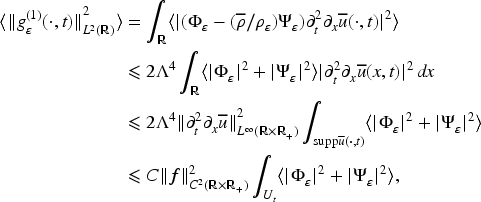
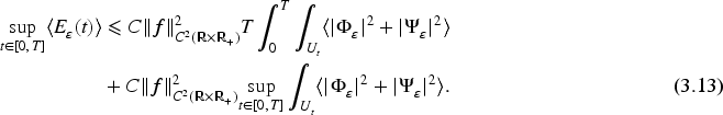
Step 4: Conclusion. Combining (3.7) and (3.10), we obtain with $C = C (Λ)$

\begin{aligned} sup_{t \in [0, T]} ⟨ E_{ε} (t) ⟩ & ⩽ C ‖ f ‖_{C^{2} (R \times R_{+})}^{2} T \int_{0}^{T} \int_{U_{t}} ⟨ | Φ_{ε} |^{2} + | Ψ_{ε} |^{2} ⟩ \\ + C ‖ f ‖_{C^{2} (R \times R_{+})}^{2} sup_{t \in [0, T]} \int_{U_{t}} ⟨ | Φ_{ε} |^{2} + | Ψ_{ε} |^{2} ⟩ . \end{aligned}

(3.13)

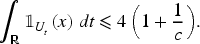
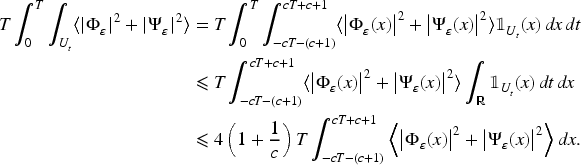
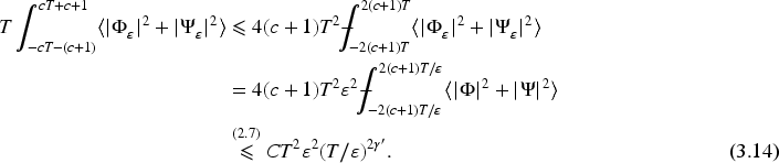
We begin by estimating the first term on the right-hand side of (3.13). For the set

U_{t} \subset [- c T - (c + 1), c T + c + 1]

we use the characteristic function

1_{U_{t}}

, defined as

1_{U_{t}} (x) = 1

x \in U_{t}

and

1_{U_{t}} (x) = 0

otherwise. The definition of

U_{t}

implies, for every

x \in R

\begin{aligned} \int_{R} 1_{U_{t}} (x) d t ⩽ 4 (1 + \frac{1}{c}) . \end{aligned}

We can therefore calculate

\begin{aligned} T \int_{0}^{T} \int_{U_{t}} ⟨ | Φ_{ε} |^{2} + | Ψ_{ε} |^{2} ⟩ & = T \int_{0}^{T} \int_{- c T - (c + 1)}^{c T + c + 1} ⟨ {| Φ_{ε} (x) |}^{2} + {| Ψ_{ε} (x) |}^{2} ⟩ 1_{U_{t}} (x) d x d t \\ ⩽ T \int_{- c T - (c + 1)}^{c T + c + 1} ⟨ {| Φ_{ε} (x) |}^{2} + {| Ψ_{ε} (x) |}^{2} ⟩ \int_{R} 1_{U_{t}} (x) d t d x \\ ⩽ 4 (1 + \frac{1}{c}) T \int_{- c T - (c + 1)}^{c T + c + 1} ⟨ {| Φ_{ε} (x) |}^{2} + {| Ψ_{ε} (x) |}^{2} ⟩ d x . \end{aligned}

At this point we exploit the growth conditions (2.7). For every

γ^{'} \in (γ, 1)

there exists

C = C (γ^{'}, Λ) \in [1, \infty)

such that, for

ε \in (0, 1]

and

T ⩾ 1

\begin{aligned} T \int_{- c T - (c + 1)}^{c T + c + 1} ⟨ | Φ_{ε} |^{2} + | Ψ_{ε} |^{2} ⟩ & ⩽ 4 (c + 1) T^{2} - \int_{- 2 (c + 1) T}^{2 (c + 1) T} ⟨ | Φ_{ε} |^{2} + | Ψ_{ε} |^{2} ⟩ \\ = 4 (c + 1) T^{2} ε^{2} - \int_{- 2 (c + 1) T / ε}^{2 (c + 1) T / ε} ⟨ | Φ |^{2} + | Ψ |^{2} ⟩ \\ \overset{(2.7)}{⩽} C T^{2} ε^{2} (T / ε)^{2 γ^{'}} . \end{aligned}

(3.14)

To estimate the second term on the right-hand side in (3.13), we use

U_{t} \subset [- c T - c - 1, c T + c + 1]

for all

t \in [0, T]

and thus for

γ^{'} \in (γ, 1)

\begin{aligned} sup_{t \in [0, T]} \int_{U_{t}} ⟨ | Φ_{ε} |^{2} + | Ψ_{ε} |^{2} ⟩ ⩽ \int_{- c T - (c + 1)}^{c T + c + 1} ⟨ | Φ_{ε} |^{2} + | Ψ_{ε} |^{2} ⟩ \overset{(3.14)}{⩽} C T ε^{2} (T / ε)^{2 γ^{'}}, \end{aligned}

where

C = C (γ^{'}, Λ) \in [1, \infty)

. Inserting in (3.13) yields the claim (3.2).

Lemma 3.1 allows to prove Part (1) of Theorem 2.6. We repeat the desired statement in the subsequent lemma. Lemma 3.2.

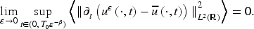
Let $(ρ, a)$ be a model of class $γ \in [0, 1)$ . Then, for all $β \in [0, \frac{1 - γ}{1 + γ})$ , classical homogenization works with parameter β in the sense of Definition 2.5.

Proof.

Because of $\frac{1 - γ}{1 + γ} = 0$ for $γ = 1$ , it suffices to consider $γ \in [0, 1)$ . Let $β \in [0, (1 - γ) / (1 + γ))$ be given and let $f \in C^{2} (R \times R_{+})$ be supported in $[- 1, 1] \times [0, 1]$ . Let $u^{ε}$ and $\bar{u}$ be the solutions of (2.3) and (2.4). We want to show that, for every $T_{0} ⩾ 1$ , there holds

\begin{aligned} \begin{matrix} lim_{ε \to 0} sup_{t \in (0, T_{0} ε^{- β})} ⟨ {‖ \partial_{t} (u^{ε} (\cdot, t) - \bar{u} (\cdot, t)) ‖}_{L^{2} (R)}^{2} ⟩ = 0. \end{matrix} \end{aligned}

By continuity, we find

γ^{'} \in (γ, 1)

such that

β \in [0, \frac{1 - γ^{'}}{1 + γ^{'}})

. The triangle inequality together with the definition

z_{ε} = u_{ε} - (\bar{u} + Φ_{ε} \partial_{x} \bar{u})

(see (3.1)) and

Λ^{- 1} ⩽ ρ_{ε} ⩽ Λ

yields

\begin{aligned} ⟨ ‖ \partial_{t} (u_{ε} (\cdot, t) - \bar{u} (\cdot, t)) ‖_{L^{2} (R)}^{2} ⟩ & ⩽ 2 ⟨ {‖ \partial_{t} z_{ε} (\cdot, t) ‖}_{L^{2} (R)}^{2} + {‖ Φ_{ε} \partial_{t} \partial_{x} \bar{u} (\cdot, t) ‖}_{L^{2} (R)}^{2} ⟩ \\ ⩽ 2 Λ ⟨ E_{ε} (t) ⟩ + 2 ⟨ {‖ Φ_{ε} \partial_{t} \partial_{x} \bar{u} (\cdot, t) ‖}_{L^{2} (R)}^{2} ⟩, \end{aligned}

(3.15)

where

E_{ε}

is defined in (3.3). We estimate the two terms on the right-hand side separately. For the first term we use Lemma 3.1 with

T = T_{0} ε^{- β}

and find a constant

C = C (γ^{'}, Λ) \in [1, \infty)

such that, for every

ε \in (0, 1]

\begin{aligned} sup_{t \in (0, T_{0} ε^{- β})} ⟨ E_{ε} (t) ⟩ & ⩽ C ε^{2 (1 - γ^{'})} (T_{0} ε^{- β})^{2 (1 + γ^{'})} ‖ f ‖_{C^{2} (R \times R_{+})}^{2} \\ = C ε^{2 (1 - β - γ^{'} (1 + β))} T_{0}^{2 (1 + γ^{'})} ‖ f ‖_{C^{2} (R \times R_{+})}^{2} . \end{aligned}

Hence,

lim_{ε \to 0} sup_{t \in (0, T ε^{- β})} ⟨ E_{ε} (t) ⟩ = 0

follows from

1 - β - γ^{'} (1 + β) > 0

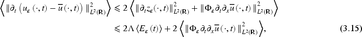
It remains to find bounds for the term $⟨ ‖ Φ_{ε} \partial_{t} \partial_{x} \bar{u} (\cdot, t) ‖_{L^{2} (R)}^{2} ⟩$ . We use computations that are similar to those of Step 3 and Step 4 in the proof of Lemma 3.1. In particular, we use that by the explicit expression (3.9) of the homogenized solution $\bar{u}$ in terms of f, which provides

\begin{aligned} ‖ \partial_{t} \partial_{x} \bar{u} ‖_{L^{\infty} (R \times R_{+})} ⩽ C ‖ f ‖_{C^{2} (R \times R_{+})} and supp u (\cdot, t) \subset U_{t}, \end{aligned}

where

C = C (Λ) \in [1, \infty)

and the set

U_{t}

is defined in (3.11). For every

t \in [0, T]

we have

supp \bar{u} (\cdot, t) \subset U_{t} \subset [- c T - c - 1, c T + c + 1]

and thus

\begin{aligned} ⟨ {‖ Φ_{ε} \partial_{t} \partial_{x} \bar{u} (\cdot, t) ‖}_{L^{2} (R)}^{2} ⟩ & = \int_{R} ⟨ | Φ_{ε} |^{2} ⟩ | \partial_{t} \partial_{x} \bar{u} (\cdot, t) |^{2} \\ ⩽ C ‖ f ‖_{C^{2} (R \times R_{+})}^{2} \int_{supp (\bar{u} (\cdot, t))} ⟨ | Φ_{ε} |^{2} ⟩ ⩽ C ‖ f ‖_{C^{2} (R \times R_{+})}^{2} \int_{- 2 (c + 1) T}^{2 (c + 1) T} ⟨ | Φ_{ε} |^{2} ⟩ \\ \overset{(3.14)}{⩽} \tilde{C} T ε^{2} (T / ε)^{2 γ^{'}}, \end{aligned}

where

\tilde{C} = \tilde{C} (γ^{'}, Λ) \in [1, \infty)

. Hence, for every

ε \in (0, 1]

and

T = T_{0} ε^{- β}

\begin{aligned} \begin{array}{rr} sup_{t \in (0, T_{0} ε^{- β})} ⟨ {‖ Φ_{ε} \partial_{t} \partial_{x} \bar{u} (\cdot, t) ‖}_{L^{2} (R)}^{2} ⟩ ⩽ \tilde{C} ε^{2 (1 - γ^{'}) - β (1 + 2 γ^{'})} T_{0}^{1 - 2 γ^{'}} ‖ f ‖_{C^{2} (R \times R_{+})} . \end{array} \end{aligned}

The right-hand side converges to zero as

ε \to 0

provided that

2 (1 - γ^{'}) - β (1 + 2 γ^{'}) > 0

, which is satisfied by the assumption

β < \frac{1 - γ^{'}}{1 + γ^{'}}

4. The upper critical parameter

In this section, we prove Part (2) of Theorem 2.6. We show that model-independent homogenization fails on large time intervals. In this result, the length of the time interval depends on the growth properties of the correctors.

The construction will be based on coordinate transformations that are given by diffeomorphisms $F : R \to R$ . We compare the wave equation in the original and in the new coordinates. We show that, when the original model defines a model of class γ, also the coefficients in the new coordinates define a model of class γ.

In Section 4.2 we use diffeomorphisms F that are based on the correctors. A relevant choice of F is given by harmonic coordinates. We stick with a more general description, since we also use a diffeomorphism F that is related to the oscillatory density coefficient. The growth properties of F imply that homogenization cannot take place for both models, the original model and the transformed model.

4.1. The wave equation in new coordinates

In this section, we use a general diffeomorphism $F : R \to R$ to define new coordinates. We always assume that F is of class $C^{1}$ and strictly monotonically increasing with a positive lower bound for the derivative.

Given F, we construct also a rescaled map: We set $F_{ε} (x) := ε F (x / ε)$ such that $\partial_{x} F_{ε} (x) = \partial_{y} F (x / ε)$ . The coordinate transformation $z = F_{ε} (x)$ is equivalent to $z / ε = F (x / ε)$ and hence equivalent to $x / ε = F^{- 1} (z / ε)$ .

Coefficients are always scaled without any multiplication with $ε$ . For coefficients in new coordinates we have, e.g.,

\begin{aligned} (ρ_{ε} \circ F^{- 1})_{ε} (z) := (ρ_{ε} \circ F^{- 1}) (z / ε) = ρ (x / ε) = ρ_{ε} (x) = ρ_{ε} \circ F_{ε}^{- 1} (z) . \end{aligned}

We next calculate the wave equation in the new coordinates $(z, t)$ .

Lemma 4.1 Transformed wave equation

Let $F : R \to R$ be a diffeomorphism. We consider new spatial coordinates in the form $z = F_{ε} (x) := ε F (x / ε)$ . Let $u^{ε}$ be a solution of the wave equation (2.3) with coefficients $ρ_{ε}$ and $a_{ε}$ . In the coordinates $(z, t)$ we consider the new function $v^{ε} := u^{ε} \circ F_{ε}^{- 1}$ . We can this as

\begin{aligned} \begin{matrix} v^{ε} \circ F_{ε} = u^{ε} o r v^{ε} (z) = u^{ε} (x) for z = F_{ε} (x) . \end{matrix} \end{aligned}

We use the transformed coefficients

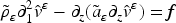
\begin{aligned} \tilde{ρ} := (ρ / \partial_{y} F) \circ F^{- 1}, \tilde{a} := (a \partial_{y} F) \circ F^{- 1}, \end{aligned}

(4.1)

which provides after $ε$ -dilation the formulas

{\tilde{ρ}}_{ε} (z) = \tilde{ρ} (z / ε) = (ρ_{ε} / \partial_{x} F_{ε}) (F_{ε}^{- 1} (z))

and

{\tilde{a}}_{ε} (z) = \tilde{a} (z / ε) = (a_{ε} \partial_{x} F_{ε}) (F_{ε}^{- 1} (z))

. Regarding the right hand side, we define

{\tilde{f}}_{ε} (z) := (f / \partial_{x} F_{ε}) (F_{ε}^{- 1} (z))

. Then the equation for

v^{ε} = v^{ε} (z, t)

reads

\begin{aligned} {\tilde{ρ}}_{ε} (z) \partial_{t}^{2} v^{ε} (z) - \partial_{z} ({\tilde{a}}_{ε} (z) \partial_{z} v^{ε} (z)) = {\tilde{f}}_{ε} (z), \end{aligned}

(4.2)

where we suppressed the argument t.

Proof.

We have to transform the terms of (2.3). In the subsequent calculations, we always omit the argument t. The spatial arguments are always related by $z = F_{ε} (x)$ . For the first term of (2.3) we find

\begin{aligned} ρ_{ε} (x) \partial_{t}^{2} u^{ε} (x) & = ρ_{ε} (x) \partial_{t}^{2} v^{ε} (z) = {\tilde{ρ}}_{ε} (z) \partial_{t}^{2} v^{ε} (z) \partial_{x} F_{ε} (F_{ε}^{- 1} (z)) . \end{aligned}

The elliptic term of (2.3) reads

\begin{aligned} \partial_{x} (a_{ε} \partial_{x} u^{ε}) (x) & = \partial_{x} (a_{ε} \partial_{x} [v^{ε} \circ F_{ε}]) (x) \\ = \partial_{x} (a_{ε} (x) \partial_{z} v^{ε} (F_{ε} (x)) \partial_{x} F_{ε} (x)) \\ = \partial_{x} ({\tilde{a}}_{ε} (F_{ε} (x)) \partial_{z} v^{ε} (F_{ε} (x))) \\ = \partial_{z} ({\tilde{a}}_{ε} (z) \partial_{z} v^{ε} (z)) \partial_{x} F_{ε} (F_{ε}^{- 1} (z)) . \end{aligned}

The right hand side of (2.3) is f. When we divide the rewritten equation (2.3) by

\partial_{x} F_{ε} (x) = \partial_{x} F_{ε} (F_{ε}^{- 1} (z))

, we obtain (4.2).

Remark 4.2 (Two problem adapted diffeomorphisms)

For two particular choices of F, the transformation yields a wave equation (4.2) that has one constant coefficient. We use the correctors Φ and $Ψ$ of (2.5).

Harmonic coordinates: Let the transformation be given by $F (y) := y + Φ (y)$ . We observe that $\partial_{y} F = 1 + \partial_{y} Φ = \bar{a} / a > 0$ . With this choice of F, we obtain $a_{ε} \partial_{x} F_{ε} = \bar{a}$ . The transformed system then has the coefficients ${\tilde{ρ}}_{ε} (z) = (ρ_{ε} a_{ε} / \bar{a}) (F_{ε}^{- 1} (z))$ and ${\tilde{a}}_{ε} (z) = \bar{a}$ for all $z \in R$ .

Coordinates for the density: With the choice $F (y) := y + Ψ (y)$ we have $\partial_{y} F = 1 + \partial_{y} Ψ = ρ / \bar{ρ} > 0$ . We find $\bar{ρ} \partial_{x} F_{ε} = ρ_{ε}$ . The transformed system has the coefficients ${\tilde{ρ}}_{ε} (z) = \bar{ρ}$ and ${\tilde{a}}_{ε} (z) = (a_{ε} ρ_{ε} / \bar{ρ}) (F_{ε}^{- 1} (z))$ for all $z \in R$ .

Let us now evaluate the homogenized coefficients in the new coordinates. Interestingly, independently of the choice of the transformation F, the homogenized coefficients remain unchanged.

The subsequent lemma yields this fact, and it contains additionally a result about the order of the transformed system. When F satisfies certain assumptions regarding its distance from the identity and when the original system has the order γ, then the system in the new coordinates has also the order γ.

Lemma 4.3 Properties of the transformed model

Let $(ρ, a)$ be a stochastic model of class $γ \in [0, 1]$ . Let $F : R \times Ω_{P} \to R$ be a family of diffeomorphisms $F (., ω) : R \to R$ . We assume that $c_{0} ⩽ \partial_{y} F (y, ω) ⩽ C_{0}$ holds for two constants $0 < c_{0} < C_{0}$ , for all $ω \in Ω_{P}$ and all y with $| y | ⩾ 1$ . We furthermore assume that, for every $γ^{'} > γ$ , there exists C such that

\begin{aligned} ⟨ - \int_{0}^{r} {| F (y, .) - y |}^{2} d y ⟩ ⩽ C {(1 + | r |^{γ^{'}})}^{2} \end{aligned}

(4.3)

for all

r \in R

. We consider the transformed coefficients

\tilde{ρ} := (ρ / \partial_{y} F) \circ F^{- 1}

and

\tilde{a} := (a \partial_{y} F) \circ F^{- 1}

. Then there holds:

(1)

The transformed model $(\tilde{ρ}, \tilde{a})$ is again of class γ.

(2)

The effective coefficients in the sense of optimal correctors are identical for the original and for the transformed model.

(3)

In the case $γ < 1$ , the effective coefficients in the sense of averages are unchanged in the sense that

\begin{aligned} lim_{| r | \to \infty} ⟨ - \int_{0}^{r} - \int_{0}^{y} \tilde{ρ} (s) d s d y ⟩ = \bar{ρ} & = lim_{| r | \to \infty} ⟨ - \int_{0}^{r} - \int_{0}^{y} ρ (s) d s d y ⟩, \end{aligned}

(4.4)

\begin{aligned} lim_{| r | \to \infty} {⟨ - \int_{0}^{r} - \int_{0}^{y} 1 / \tilde{a} (s) d s d y ⟩}^{- 1} = \bar{a} & = lim_{| r | \to \infty} {⟨ - \int_{0}^{r} - \int_{0}^{y} 1 / a (s) d s d y ⟩}^{- 1} . \end{aligned}

(4.5)

Proof.

Step 1: $L^{2}$ -norm in transformed coordinates. The upper and lower bounds $C_{0}$ and $c_{0}$ on the growth of F imply that $L^{2}$ -norms in transformed coordinates are equivalent to $L^{2}$ -norms in original coordinates. More precisely, for any $L^{2}$ -function $g : R \to R$ and any integration bounds $0 < r < R$ , there holds, with the substitution $p = F (s)$ ,

\begin{aligned} \int_{r}^{R} | g \circ F |^{2} (s) d s = \int_{F (r)}^{F (R)} {| g (p) |}^{2} {| \partial_{y} F (F^{- 1} (p)) |}^{- 1} d p ⩽ c_{0}^{- 1} \int_{c_{0} r}^{C_{0} R} {| g (p) |}^{2} . \end{aligned}

(4.6)

A similar calculation can be performed for a lower bound and for the inverse transformation.

Step 2: Assertions 1. and 2. The main point is that the transformed system is of class γ, but the subsequent calculation provides also that the effective coefficients are not changed. We fix $γ^{'} > γ$ . We define the corrector $\tilde{Ψ}$ with the transformed coefficient $\tilde{ρ}$ and the same number $\bar{ρ}$ . We calculate, with the change of coordinates $p = F (s)$ in the second line,

\begin{aligned} \tilde{Ψ} (y) & := \int_{0}^{y} {\frac{\tilde{ρ} (p)}{\bar{ρ}} - 1} d p = \frac{1}{\bar{ρ}} \int_{0}^{y} (ρ / \partial_{y} F) (F^{- 1} (p)) d p - y \\ = \frac{1}{\bar{ρ}} \int_{0}^{F^{- 1} (y)} ρ (s) d s - y \\ = \int_{0}^{F^{- 1} (y)} {\frac{ρ (s)}{\bar{ρ}} - 1} d s + (F^{- 1} (y) - y) \\ = Ψ (F^{- 1} (y)) + (F^{- 1} (y) - y) . \end{aligned}

We now exploit that, for some

C > 0

and all

r > 0

, the growth estimate holds for the original model:

⟨ - \int_{0}^{r} | Ψ (y) |^{2} d y ⟩ ⩽ C (1 + | r |^{γ^{'}})^{2}

. Evaluating the corresponding expression for the first term of

\tilde{Ψ} (y)

, we get

\begin{aligned} ⟨ - \int_{0}^{r} {| Ψ (F^{- 1} (y)) |}^{2} d y ⟩ ⩽ \frac{C_{0}}{c_{0}} ⟨ - \int_{0}^{c_{0}^{- 1} r} {| Ψ (y) |}^{2} d y ⟩ ⩽ \frac{C C_{0}}{c_{0}} (1 + | c_{0}^{- 1} r |^{γ^{'}})^{2} . \end{aligned}

Regarding the second term we obtain with the Cauchy–Schwarz inequality

\begin{aligned} {| ⟨ - \int_{0}^{r} (F^{- 1} (y) - y) d y ⟩ |}^{2} & ⩽ ⟨ - \int_{0}^{r} {| F^{- 1} (y) - y |}^{2} d y ⟩ \\ ⩽ \frac{C_{0}}{c_{0}} ⟨ - \int_{0}^{c_{0}^{- 1} r} {| s - F (s) |}^{2} d s ⟩ ⩽ \frac{C C_{0}}{c_{0}} (1 + | r |^{γ^{'}})^{2}, \end{aligned}

where we used (4.3) in the last inequality. We conclude that there exists

C < \infty

such that

\begin{aligned} ⟨ - \int_{0}^{r} {| \tilde{Ψ} (y) |}^{2} d y ⟩ ⩽ C {(1 + | r |^{γ^{'}})}^{2} \end{aligned}

(4.7)

and thus the claim for

\tilde{Ψ}

. The same calculation can be performed for Φ. Since

γ^{'} > γ

was arbitrary, we conclude that the transformed model has an order not greater than γ.

Since the argument can be also used in the opposite direction, we also know that the class γ of the original problem is less than or equal to the class of the transformed system. This shows that the two classes actually coincide. Since we have used the numbers $\bar{ρ}$ and $\bar{a}$ of the original model in the calculation, we have obtained also the second assertion.

Step 3: Effective coefficients in the sense of averages. The subsequent lemma provides Assertion 3. Loosely speaking, the lemma shows that, for $γ < 1$ , the effective coefficients in the sense of averages coincide with the effective coefficients in the sense of optimal correctors.

Lemma 4.4 On the two definitions of effective coefficients

Let $(ρ, a)$ be a stochastic model of class $γ \in [0, 1)$ . Let $\bar{ρ}, \bar{a} \in R$ be such that the corresponding correctors have the following property: For every $γ^{'} > γ$ there is $C > 0$ such that, for all $r \in R$ ,

\begin{aligned} ⟨ - \int_{0}^{r} {| Φ (y) |}^{2} d y ⟩ + ⟨ - \int_{0}^{r} {| Ψ (y) |}^{2} d y ⟩ ⩽ C {(1 + | r |^{γ^{'}})}^{2} . \end{aligned}

(4.8)

Then the effective coefficients in the sense of averages are well-defined and coincide with

\bar{ρ}

and

\bar{a}

Proof.

We perform all calculations for ρ and $Ψ$ , the calculations for a and Φ are analogous. Furthermore, we can restrict ourselves to $r > 0$ , the calculations for negative r are identical. Because of $γ < 1$ we can furthermore assume $γ^{'} < 1$ . Our goal is to study the expression

\begin{aligned} ρ_{*} & := lim_{r \to \infty} ⟨ - \int_{0}^{r} - \int_{0}^{y} ρ (s) d s d y ⟩ = lim_{r \to \infty} ⟨ - \int_{0}^{r} \frac{\bar{ρ}}{y} (Ψ (y) + y) d y ⟩ \\ = \bar{ρ} + lim_{r \to \infty} ⟨ - \int_{0}^{r} \frac{\bar{ρ}}{y} Ψ (y) d y ⟩ . \end{aligned}

The lemma is proven when we show that the limit in the last line exists and that it vanishes.

With this aim, we use a dyadic decomposition of the integral. For a large number r, we select the natural number K with $r \in (2^{K - 1}, 2^{K}]$ . With constants C that depend only on the upper bound of ρ, we calculate for the squared absolute value with the Cauchy–Schwarz inequality

\begin{aligned} {| ⟨ - \int_{0}^{r} \frac{1}{y} Ψ (y) d y ⟩ |}^{2} & ⩽ ⟨ - \int_{0}^{r} {| \frac{1}{y} Ψ (y) |}^{2} d y ⟩ ⩽ \frac{C}{r} + \frac{1}{r} ⟨ \int_{1}^{2^{K}} {| \frac{1}{y} Ψ (y) |}^{2} d y ⟩ \\ ⩽ C \frac{1}{2^{K - 1}} + \frac{1}{2^{K - 1}} \sum_{k = 1}^{K} {| \frac{1}{2^{k - 1}} |}^{2} ⟨ \int_{2^{k - 1}}^{2^{k}} {| Ψ (y) |}^{2} d y ⟩ . \end{aligned}

Using estimate (4.8) with

r = 2^{k}

we find, with the constant C changing in the last inequality,

\begin{aligned} ⟨ \int_{2^{k - 1}}^{2^{k}} {| Ψ (y) |}^{2} d y ⟩ ⩽ 2^{k} ⟨ - \int_{0}^{2^{k}} {| Ψ (y) |}^{2} d y ⟩ ⩽ 2^{k} C (1 + | 2^{k} |^{γ^{'}})^{2} ⩽ C 2^{k (1 + 2 γ^{'})} . \end{aligned}

Inserting above we obtain

\begin{aligned} {| ⟨ - \int_{0}^{r} \frac{1}{y} Ψ (y) d y ⟩ |}^{2} & ⩽ C 2^{- K} + C 2^{- K} \sum_{k = 1}^{K} 2^{- 2 k} 2^{k (1 + 2 γ^{'})} \\ ⩽ C 2^{- K} + C 2^{- K} \sum_{k = 1}^{K} 2^{k (2 γ^{'} - 1)} . \end{aligned}

For

γ^{'} ⩽ 1 / 2

, this tends obviously to zero for

K \to \infty

. For

γ^{'} \in (1 / 2, 1)

, the second expression can be estimated by

\begin{aligned} 2^{- K} \sum_{k = 1}^{K} 2^{k (2 γ^{'} - 1)} ⩽ C 2^{- K} 2^{K (2 γ^{'} - 1)} ⩽ C 2^{K (2 γ^{'} - 2)}, \end{aligned}

which tends to zero because of

γ^{'} < 1

. This shows

ρ_{*} = \bar{ρ}

and hence the claim.

4.2. Failure of stochastic homogenization

We claim that stochastic homogenization must fail on large time scales. The principal approach to the proof can be described as follows. We fix a model class parameter γ and fix a parameter β beyond the critical threshold $β_{+}$ . Let us assume that homogenization works with the parameter β. We consider a model $(ρ, a)$ of class γ. Then, for any $γ^{'} > γ$ , a change of coordinates provides a new model $(\tilde{ρ}, \tilde{a})$ that satisfies the corrector estimates with parameter $γ^{'}$ , hence the new model is again of class γ. Then both models, the old one, $(ρ, a)$ , and the new one, $(\tilde{ρ}, \tilde{a})$ , allow homogenization. On the other hand, the coordinate transformation has a growth that is essentially γ, and this fact yields a contradiction to the fact that the $ε$ -solutions of both models are close to the homogenized solution (and hence close to each other).

Proposition 4.5 Upper critical parameter

Let $γ \in (0, 1)$ be such that a model with this model class parameter exists. Then

\begin{aligned} β_{+} := \frac{1 - γ}{γ} \end{aligned}

is an upper critical parameter in the sense of Theorem 2.6: For any

β \in (β_{+}, \infty)

there are coefficients

(ρ, a)

of class γ such that classical homogenization does not work with parameter β.

Proof.
Step 0: Preparation. We perform a proof by contradiction. We assume that, for some $β > β_{+}$ , classical homogenization works with parameter β for all coefficients $(ρ, a)$ of class γ. From now on we consider γ and $β > β_{+}$ as fixed and wish to derive a contradiction. Because of $β > β_{+}$ we can choose a number $0 < \tilde{γ} < γ$ such that $\tilde{γ} (1 + β) > 1$ .

We furthermore choose a model $(ρ, a)$ of class γ. The contradiction will be derived from the fact that homogenization cannot work simultaneously for $(ρ, a)$ and the transformed model $(\tilde{ρ}, \tilde{a})$ .

In the proof, we fix some function f, consider rescaled stochastic coefficients $ρ_{ε} (x) = ρ (x / ε)$ and $a_{ε} (x) = a (x / ε)$ , and study the solution $u^{ε}$ of the wave equation (1.1) for $f_{ε} = f$ with trivial initial data. Another object is the solution $\bar{u}$ of the effective wave equation
$\begin{aligned} \bar{ρ} \partial_{t}^{2} \bar{u} - \bar{a} \partial_{x}^{2} \bar{u} = f, \end{aligned}$
(4.9)
with trivial initial data. Since, by assumption, classical homogenization works for the parameter β, we know that $u^{ε} - \bar{u} \to 0$ holds in the sense of (2.9): For every $T_{0} > 0$ , as $ε \to 0$ ,
$\begin{aligned} sup_{t \in (0, T_{0} ε^{- β})} ⟨ {‖ \partial_{t} u^{ε} (., t) - \partial_{t} \bar{u} (., t) ‖}_{L^{2} (R)} ⟩ \to 0. \end{aligned}$
(4.10)

Step 1: The limit solution. Let us first make a choice for the right hand side f. We choose a smooth non-negative function f with support in $[- 1, 1] \times [0, 1]$ which satisfies $f > 0$ on $[- 3 / 4, 3 / 4] \times [1 / 4, 3 / 4]$ . The generalized d’Alembert representation formula in one space dimension allows to write the solution $\bar{u}$ with the help of integrals over f. With $c^{2} = \bar{a} / \bar{ρ}$ and initial data $\bar{u} (\cdot, 0) = \partial_{t} \bar{u} (\cdot, 0) \equiv 0$ , the limit solution reads
$\begin{aligned} \bar{u} (x, t) = \frac{1}{2 c \bar{ρ}} \int_{0}^{t} \int_{x - c (t - s)}^{x + c (t - s)} f (x^{'}, s) d x^{'} d s . \end{aligned}$
(4.11)
The formula implies that, for every time instance $t > 0$ , the function $\bar{u} (., t)$ has its support in $[- c t - (1 + c), - c t + (1 + c)] \cup [c t - (1 + c), c t + (1 + c)]$ . The function $\bar{u} (., t)$ is positive in the point $x = c t$ , and non-negative everywhere. Loosely speaking, $\bar{u}$ is a combination of two wave pulses, both positive, one located at $x = c t$ and the other located at $x = - c t$ .

Step 2: Model class γ. Since $(ρ, a)$ is of class γ, the parameter $\tilde{γ}$ is below the infimum over admissible growth rates, $\tilde{γ} < γ = inf Γ_{s c}$ ; this implies that, considering the constants $C_{k} = k \in N$ ,
$\begin{aligned} \exists r = r_{k} \in R : ⟨ - \int_{0}^{r} {| Φ (y) |}^{2} d y ⟩ + ⟨ - \int_{0}^{r} {| Ψ (y) |}^{2} d y ⟩ > 2 C_{k} {(1 + | r |^{\tilde{γ}})}^{2} . \end{aligned}$
(4.12)
Because of (4.12), we can choose a subsequence $k \to \infty$ such that
$\begin{aligned} \forall k : ⟨ - \int_{0}^{r_{k}} {| Φ (y) |}^{2} d y ⟩ > C_{k} (1 + {| r_{k} |}^{\tilde{γ}})^{2} or \forall k : ⟨ - \int_{0}^{r_{k}} {| Ψ (y) |}^{2} d y ⟩ > C_{k} (1 + {| r_{k} |}^{\tilde{γ}})^{2} . \end{aligned}$
In the following, we suppose that there exists a sequence $k \to \infty$ such that
$\begin{aligned} ⟨ - \int_{0}^{r_{k}} {| Ψ (y) |}^{2} d y ⟩ > C_{k} {(1 + | r_{k} |^{\tilde{γ}})}^{2} \end{aligned}$
(4.13)
(the case in which (4.13) holds with $Ψ$ replaced by Φ can be treated analogously). For large k, there must hold $r_{k} ⩾ 2$ , so we always assume this lower bound in the following. We claim that, for every $k \in N$ with $r_{k} ⩾ 2$ it holds
$\begin{aligned} \exists y_{k} \in [r_{k} / 2, r_{k}] : ⟨ {| Ψ (y_{k}) |}^{2} ⟩ > C_{k} {(1 + | y_{k} |^{\tilde{γ}})}^{2} . \end{aligned}$
(4.14)

Indeed, assuming that (4.14) fails to hold, we have
$\begin{aligned} \int_{0}^{r_{k}} ⟨ {| Ψ (y) |}^{2} ⟩ d y ⩽ \int_{r_{k} / 2}^{r_{k}} ⟨ {| Ψ (y) |}^{2} ⟩ d y ⩽ \frac{r_{k}}{2} C_{k} (1 + | r_{k} |^{\tilde{γ}})^{2}, \end{aligned}$
in contradiction to (4.13) (recall $r_{k} ⩾ 2$ ).

We choose the transformation $F := id + Ψ$ . Inequality (4.14) reads
$\begin{aligned} ⟨ {| F (y_{k}) - y_{k} |}^{2} ⟩ > C_{k} {(1 + | y_{k} |^{\tilde{γ}})}^{2} . \end{aligned}$
(4.15)
In this sense, the coordinate transformation produces large errors at some points.

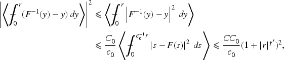
Let us now exploit in another way that the model class is γ. For every $γ^{'} > γ$ there exists a constant C such that
$\begin{aligned} ⟨ - \int_{0}^{r} {| F (y, .) - y |}^{2} d y ⟩ = ⟨ - \int_{0}^{r} {| Ψ (y) |}^{2} d y ⟩ ⩽ C {(1 + | r |^{γ^{'}})}^{2} \end{aligned}$
(4.16)
for all $r \in R$ . Property (4.16) corresponds to one of the assumptions on F in Lemma 4.3. The other assumption reads $0 < c_{0} ⩽ F (y, ω) / y ⩽ C_{0}$ and follows from the fact that
$\begin{aligned} \partial_{y} F (y) = 1 + \partial_{y} Ψ (y) = \frac{ρ (y)}{\bar{ρ}} \in [\frac{m_{ρ}}{\bar{ρ}}, \frac{M_{ρ}}{\bar{ρ}}], \end{aligned}$
(4.17)
and similarly in the case that $\partial_{y} F (y) = 1 + \partial_{y} Φ (y)$ .

Step 3: Transformation of the equation. We recall that the model $(ρ, a)$ and the coordinate change F are fixed. We use the transformation of Lemma 4.1. The function $v^{ε}$ is defined by $v^{ε} \circ F_{ε} = u^{ε}$ , the new coefficients are ${\tilde{ρ}}_{ε} (z) := (ρ_{ε} / \partial_{x} F_{ε}) (F_{ε}^{- 1} (z))$ and ${\tilde{a}}_{ε} (z) := (a_{ε} \partial_{x} F_{ε}) (F_{ε}^{- 1} (z))$ , the new sources are ${\tilde{f}}_{ε} (z) := (f / \partial_{x} F_{ε}) (F_{ε}^{- 1} (z))$ . The transformed equation is given by (4.2),
$\begin{aligned} {\tilde{ρ}}_{ε} (z) \partial_{t}^{2} v^{ε} (z) - \partial_{z} ({\tilde{a}}_{ε} (z) \partial_{z} v^{ε} (z)) = {\tilde{f}}_{ε} (z), \end{aligned}$
(4.18)
and $v^{ε}$ satisfies trivial initial conditions. Because of (4.16) with arbitrary $γ^{'} > γ$ , Lemma 4.3 yields that $\tilde{ρ}$ and $\tilde{a}$ define again a model of class γ and that the homogenized system is again given by $\bar{ρ}$ and $\bar{a}$ . By our assumption, classical homogenization works with parameter β also for the coefficients $(\tilde{ρ}, \tilde{a})$ . This implies that the solutions ${\hat{v}}^{ε}$ of
$\begin{aligned} {\tilde{ρ}}_{ε} \partial_{1}^{2} {\hat{v}}^{ε} - \partial_{z} ({\tilde{a}}_{ε} \partial_{z} {\hat{v}}^{ε}) = f \end{aligned}$
with zero initial conditions satisfy, as $ε \to 0$ ,
$\begin{aligned} sup_{t \in (0, T_{0} ε^{- β})} ⟨ {‖ \partial_{t} {\hat{u}}^{ε} (\cdot, t) - \partial_{t} \bar{u} (, \cdot t) ‖}_{L^{2} (R)} ⟩ \to 0, \end{aligned}$
(4.19)
just as $u^{ε}$ in (4.10).

Step 4: Only a small error is introduced by changing from ${\tilde{f}}_{ε}$ to f. This step is slightly technical. Let $v^{ε}$ and ${\hat{v}}^{ε}$ be as in Step 3. We consider the difference $w^{ε} := v^{ε} - {\hat{v}}^{ε}$ and claim that
$\begin{aligned} lim_{ε \to 0} sup_{t \in (0, T_{0} ε^{- β})} ⟨ {‖ \partial_{t} w^{ε} (\cdot, t) ‖}_{L^{2} (R)} ⟩ = 0. \end{aligned}$
(4.20)
Note that (4.20) together with (4.19) implies
$\begin{aligned} lim_{ε \to 0} sup_{t \in (0, T_{0} ε^{- β})} ⟨ {‖ \partial_{t} υ^{ε} (\cdot, t) - \partial_{t} \bar{υ} (\cdot, t) ‖}_{L^{2} (2 R)} ⟩ \to 0. \end{aligned}$
(4.21)
We will exploit this property in the next step of the proof.

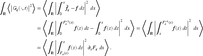
To derive (4.20), we start from the equation for $w^{ε}$ ,
$\begin{aligned} \begin{matrix} ◻_{ε} w^{ε} = {\tilde{f}}_{ε} - f =: g_{ε} . \end{matrix} \end{aligned}$
In view of Lemma B.1, it suffices to show for the space integrals $G_{ε} (x, t, ω) = \int_{0}^{x} g_{ε} (s, t, ω) d s$ the convergence
$\begin{aligned} sup_{t ⩾ 0} \int_{R} ⟨ {| G_{ε} (\cdot, t) |}^{2} ⟩ + ⟨ {| \partial_{t} G_{ε} (\cdot, t) |}^{2} ⟩ d x \to 0 \end{aligned}$
(4.22)
as $ε \to 0$ . We compute for $x > 0$ and omit the argument t after the first equality,
$\begin{aligned} \int_{R} ⟨ {| G_{ε} (\cdot, t) |}^{2} ⟩ & = ⟨ \int_{R} {| \int_{0}^{x} {\tilde{f}}_{ε} - f d s |}^{2} d x ⟩ \\ = ⟨ \int_{R} {| \int_{0}^{F_{ε}^{- 1} (x)} f (s) d s - \int_{0}^{x} f (s) d s |}^{2} d x ⟩ = ⟨ \int_{R} {| \int_{x}^{F_{ε}^{- 1} (x)} f (s) d s |}^{2} d x ⟩ \\ = ⟨ \int_{R} {| \int_{F_{ε} (x)}^{x} f (s) d s |}^{2} \partial_{x} F_{ε} d x ⟩ . \end{aligned}$
We consider the case $F (y) = y + Ψ (y)$ . Equation (4.17) together with $F (0) = 0$ imply the deterministic lower bound $| F_{ε} (x) | ⩾ \frac{m_{ρ}}{\bar{ρ}} | x |$ for all $x \in R$ and $ω \in Ω_{P}$ . Hence, $supp f (\cdot, t) \subset [- 1, 1]$ implies that
$\begin{aligned} | \int_{F_{ε} (x)}^{x} f (s) d s | = 0 for every x with | x | ⩾ 1 + \frac{m_{ρ}}{\bar{ρ}} . \end{aligned}$
We therefore obtain with $R := 1 + \frac{m_{ρ}}{\bar{ρ}}$ ,
$\begin{aligned} \int_{R} ⟨ {| G_{ε} (\cdot, t) |}^{2} ⟩ & = ⟨ \int_{- R}^{R} {| \int_{F_{ε} (x)}^{x} f (s) d s |}^{2} \partial_{x} F_{ε} d x ⟩ \\ ⩽ \frac{M_{ρ}}{\bar{ρ}} | | f | |_{L^{\infty}}^{2} ⟨ \int_{- R}^{R} {| Ψ_{ε} (x) |}^{2} d x ⟩ = \frac{M_{ρ}}{\bar{ρ}} | | f | |_{L^{\infty}}^{2} ε^{3} \int_{- R / ε}^{R / ε} ⟨ {| Ψ |}^{2} ⟩ \\ = \frac{2 R M_{ρ}}{\bar{ρ}} | | f | |_{L^{\infty}}^{2} ε^{2} - \int_{- R / ε}^{R / ε} ⟨ {| Ψ |}^{2} ⟩ \to 0 \end{aligned}$
as $ε \to 0$ . In the convergence of the last line we exploited the sublinear growth of $Ψ$ (compare, e.g., (4.16), and note that we can choose $γ < γ^{'} < 1$ ). The time derivative of $G_{ε}$ in (4.22) is treated with the same calculation, replacing f by $\partial_{t} f$ .

Step 5: Derivation of a contradiction. The remainder of this proof uses the following observation: By the error estimates (4.10) and (4.21), $u^{ε}$ and $v^{ε}$ are close to each other. This is in contradiction with the definition of $v^{ε}$ through $v^{ε} \circ F_{ε} = u^{ε}$ and the large deviation (4.15) of the transformation at the points $y_{k}$ .

Let us turn to the details of the argument. In Step 2 of this proof, we have constructed a sequence of points $y_{k}$ such that $⟨ | F (y_{k}) - y_{k} |^{2} ⟩ > k (1 + | y_{k} |^{\tilde{γ}})^{2}$ , see (4.15). Since F remains bounded on bounded sets by the upper bound on $| \partial_{y} F |$ , we know that necessarily $| y_{k} | \to \infty$ . Given the sequence $y_{k}$ , we choose the sequence $ε_{k} := | y_{k} |^{- 1 / (1 + β)}$ . The choice is made such that $ε_{k}^{1 + β} | y_{k} | = 1$ , and hence $ε_{k} | y_{k} | = ε_{k}^{- β}$ . Upon choosing a subsequence, we can assume that all points $y_{k}$ have the same sign; without loss of generality we assume that the sign is positive. We consider the rescaled points $x_{k} := ε_{k} y_{k} = ε_{k}^{- β}$ and the time instances $t_{k} := x_{k} / c$ with $c = \sqrt{\bar{a} / \bar{ρ}}$ as introduced above.

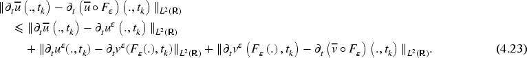
The overall picture is that the functions $u^{ε} \approx \bar{u} = \bar{v} \approx v^{ε}$ must all have a pulse at position $x_{k}$ at time $t_{k}$ . Let us quantify this statement. Writing short $ε = ε_{k}$ , the triangle inequality and $\bar{u} = \bar{v}$ yield
$\begin{aligned} ‖ \partial_{t} \bar{u} (., t_{k}) - \partial_{t} (\bar{u} \circ F_{ε}) (., t_{k}) ‖_{L^{2} (R)} \\ ⩽ ‖ \partial_{t} \bar{u} (., t_{k}) - \partial_{t} u^{ε} (., t_{k}) ‖_{L^{2} (R)} \\ + ‖ \partial_{t} u^{ε} (., t_{k}) - \partial_{t} v^{ε} (F_{ε} (.), t_{k}) ‖_{L^{2} (R)} + ‖ \partial_{t} v^{ε} (F_{ε} (.), t_{k}) - \partial_{t} (\bar{v} \circ F_{ε}) (., t_{k}) ‖_{L^{2} (R)} . \end{aligned}$
(4.23)
The second term on the right hand side was introduced to make the calculation clear; it vanishes identically. Taking expectations, (4.10) provides convergence to 0 as $k \to \infty$ for the first term on the right hand side. In the third term we can exploit the upper and lower bounds $c_{0}$ and $C_{0}$ on the growth of F. Such bounds imply that the $L^{2}$ -norm in transformed coordinates is equivalent to the original coordinates in the sense of (4.6). This allows to estimate the third term by $C ‖ \partial_{t} v^{ε} (., t_{k}) - \partial_{t} \bar{v} (., t_{k}) ‖_{L^{2} (R)}$ , which vanishes after taking expectations in the limit $ε \to 0$ by (4.21). Altogether, we obtain from (4.23) for the expected value
$\begin{aligned} ⟨ {‖ \partial_{t} \bar{u} (\cdot, t_{k}) - \partial_{t} (\bar{u} \circ F_{ε}) (\cdot, t_{k}) ‖}_{L^{2} (R)} ⟩ \to 0. \end{aligned}$
(4.24)

We want to lead (4.24) to a contradiction with the fact that the function $\partial_{t} \bar{u} (., t_{k})$ has non-trivial values in a neighborhood of $x_{k}$ , but vanishing values at positive points that are more than $O (1)$ away from $x_{k}$ .

The transformation satisfies $⟨ | F (y_{k}) - y_{k} |^{2} ⟩ > k | y_{k} |^{2 \tilde{γ}}$ by (4.15). Given this lower bound for the expected value, there necessarily exists a subset $Ω_{1} \subset Ω_{P}$ of events with positive measure, $P (Ω_{1}) = p_{1} > 0$ such that $| F (y_{k}, ω) - y_{k} |^{2} > k | y_{k} |^{2 \tilde{γ}}$ for all $ω \in Ω_{1}$ .

We calculate the mismatch in $ε$ -rescaled variables, writing again short $ε$ instead of $ε_{k}$ . Because of $x_{k} := ε y_{k}$ , $F_{ε} (x_{k}) = ε F (y_{k})$ , and $ε := | y_{k} |^{- 1 / (1 + β)}$ , we find, for $ω \in Ω_{1}$ ,
$\begin{aligned} | F_{ε} (x_{k}, ω) - x_{k} | = ε | F (y_{k}, ω) - y_{k} | ⩾ ε \sqrt{k} | y_{k} |^{\tilde{γ}} = \sqrt{k} ε^{1 - \tilde{γ} (1 + β)} . \end{aligned}$
(4.25)
We had chosen $\tilde{γ}$ in Step 0 such that $\tilde{γ} (1 + β) > 1$ . Because of this choice, the exponent in the last expression of (4.25) is negative, which means that the mismatch $| F_{ε} (x_{k}, ω) - x_{k} |$ is arbitrarily large.

This provides a contradiction with (4.24). For every $ω \in Ω_{1}$ , the function $\partial_{t} \bar{u} (., t_{k})$ has its support (on the positive axis) around the point $x_{k}$ . On the other hand, $\partial_{t} (\bar{u} \circ F_{ε}) (., t_{k})$ vanishes around the point $x_{k}$ because of (4.25). Being a fixed positive quantity on a set with positive measure, and being non-negative everywhere, the expectation of the norm in (4.24) cannot vanish in the limit. We have found the desired contradiction.

5. Sharp homogenization results for matched impedance

Let us introduce a stochastic medium with matched impedance. As in Section 2.3, we focus on the situations of i.i.d. coefficients. Extensions to correlated coefficients are possible, see Remark 5.2 below. Fix $Λ > 1$ and let $a : Z \times Ω_{P} \to [Λ^{- 1}, Λ]$ be such that the random variables $(a_{j})_{j \in Z}$ with $a_{j} := a (j, \cdot)$ are i.i.d.. We define the random coefficients $ρ, a : R \times Ω_{P} \to [Λ^{- 1}, Λ]$ by

\begin{aligned} \begin{matrix} a (x, ω) := a_{j} (ω), ρ (x, ω) := \frac{1}{a_{j} (ω)} for x \in [j, j + 1) . \end{matrix} \end{aligned}

The rescaled coefficients are

a_{ε} := a (\cdot / ε)

and

ρ_{ε} := ρ (\cdot / ε)

Theorem 5.1 Critical parameter for media with matched impedance

Let the stochastic medium $(ρ, a)$ be as described above. Then $ε^{- 1}$ is the critical time horizon for classical homogenization in the following sense:

(1)
Let $β > 1$ and $T_{0} > 0$ be two numbers. Let $f : R \times [0, \infty) \to R$ be supported on $[- 1, 1] \times (0, 1)$ with the property that the corresponding homogenized solution does not have compact support. Then the solution $u^{ε}$ of (2.3) and the solution $\bar{u}$ of (2.4) satisfy
$\begin{aligned} \underset{ε \to 0}{lim sup} sup_{t \in (0, T_{0} ε^{- β})} ⟨ {‖ \partial_{t} u^{ε} (., t) - \partial_{t} \bar{u} (., t) ‖}_{L^{2} (R)} ⟩ > 0. \end{aligned}$
(5.1)
(2)
Let $0 ⩽ β < 1$ and $T_{0} > 0$ be two numbers. Let $f : R \times [0, \infty) \to R$ be smooth and supported on $[- 1, 1] \times (0, 1)$ . Then the solutions $u^{ε}$ and $\bar{u}$ satisfy
$\begin{aligned} \underset{ε \to 0}{lim sup} sup_{t \in (0, T_{0} ε^{- β})} ⟨ {‖ \partial_{t} u^{ε} (., t) - \partial_{t} \bar{u} (., t) ‖}_{L^{2} (R)} ⟩ = 0. \end{aligned}$
(5.2)

Proof of Part (1) of Theorem 5.1. Proof of Part (1) of Theorem 5.1.

The underlying idea of the proof is to use the exact solutions to the homogeneous wave equation with piecewise constant coefficients of (2.12). We recall that a matched impedance is needed in order to have explicit solution in that form.

We allow here not only a right-going wave (with shape function g), but additionally a left-going wave (with shape function h). For times $t > 1$ , the function $u^{ε}$ solves a wave equation with vanishing right hand side. This allows to express $u^{ε}$ with g and h. Writing $v^{ε}$ instead of $u^{ε}$ for times $t > 1$ , and allowing that g and h depend also on $ε$ , an adaption of formula (2.12) reads

\begin{aligned} v^{ε} (x, t) := g^{ε} (\frac{x - ε j}{a_{j}} - t + \sum_{i = 0}^{j - 1} \frac{ε}{a_{i}}) + h^{ε} (\frac{x - ε j}{a_{j}} + t + \sum_{i = 0}^{j - 1} \frac{ε}{a_{i}}) \end{aligned}

(5.3)

for

x \in [ε j, ε (j + 1))

. On the other hand, a comparable solution

\bar{v}

of the homogenized equation with

\bar{ρ}

and

\bar{a}

reads, compare (2.14):

\begin{aligned} \bar{v} (x, t) := \bar{g} (\frac{x}{\bar{a}} - t) + \bar{h} (\frac{x}{\bar{a}} + t) . \end{aligned}

(5.4)

When we include also left-going waves, we do not only have that

v^{ε}

and

\bar{v}

are solutions to the corresponding homogeneous wave equations, but, moreover, every solution of the one-dimensional wave equation can be written with appropriate

g^{ε}

h^{ε}

\bar{g}

, and

\bar{h}

in the above form.

Our proof relies on two observations. (i) For appropriate g- and h-functions, there holds, for $t > 1$ : $u^{ε} = v^{ε}$ and $\bar{u} = \bar{v}$ with $g^{ε} \approx \bar{g}$ and $h^{ε} \approx \bar{h}$ . (ii) For large times, solutions $v^{ε}$ and $\bar{v}$ have their main wave pulses at very distant points. This implies (5.1).

Step 0: Preparation. We fix the right hand side f with support on $[- 1, 1] \times (0, 1)$ as in the Theorem and $β > 1$ . We perform a proof with a contradiction argument and assume that convergence holds in (5.1), i.e., as $ε \to 0$ ,

\begin{aligned} sup_{t \in (0, T_{0} ε^{- β})} ⟨ {‖ \partial_{t} u^{ε} (., t) - \partial_{t} \bar{u} (., t) ‖}_{L^{2} (R)} ⟩ \to 0. \end{aligned}

(5.5)

Step 1: Representation of $u^{ε}$ and $\bar{u}$ . The function $\bar{u} = \bar{u} (x, t)$ is a solution of the homogeneous wave equation ${\bar{a}}^{- 1} \partial_{t}^{2} \bar{u} - \bar{a} \partial_{x}^{2} \bar{u} = 0$ for $t > 1$ . We can therefore, for appropriate functions $\bar{g}$ and $\bar{h}$ , write $\bar{u}$ in the form of (5.4): $\bar{u} (x, t) = \bar{v} (x, t)$ for $t > 1$ for $\bar{v}$ as in (5.4). This defines $\bar{g}$ and $\bar{h}$ . Indeed, by Lemma A.1, we have for $t > 1$

\begin{aligned} \bar{u} (x, t) & = \frac{1}{2} (g (\frac{x}{\bar{a}} - (t - 1)) + g (\frac{x}{\bar{a}} + (t - 1))) + \frac{1}{2} \int_{\frac{x}{\bar{a}} - t - 1}^{\frac{x}{\bar{a}} + t - 1} h (y) d y, \end{aligned}

where g and h are given by

\bar{u} (x, 1) = g (\frac{x}{\bar{a}})

and

\partial_{t} \bar{u} (x, 1) = h (\frac{x}{\bar{a}})

. The above representation formula can be rewritten as a sum of two pulses as in (5.4) by setting

\begin{aligned} \bar{g} (s) := \frac{1}{2} g (s + 1) - \frac{1}{2} \int_{- \infty}^{s + 1} h (y) d y, \bar{h} (s) := \frac{1}{2} g (s - 1) + \frac{1}{2} \int_{- \infty}^{s - 1} h (y) d y . \end{aligned}

Note that

\bar{g} \neq 0

\bar{h} \neq 0

holds by assumption on f. For fixed

ε > 0

, we can also use a representation formula for

u^{ε}

. As a solution of a homogeneous wave equation with coefficients

ρ_{ε}

and

a_{ε}

for

t > 1

, there exist functions

g^{ε} : R \to R

and

h^{ε} : R \to R

such that

u^{ε}

has the form of (5.3),

u^{ε} (x, t) = v^{ε} (x, t)

for

t > 1

for

v^{ε}

as in (5.3). This defines

g^{ε}

and

h^{ε}

. This fact and precise expressions for

g^{ε}

and

h^{ε}

can be derived as above for

\bar{g}

and

\bar{h}

appealing to the d’Alambert-type representation formula for solutions of the wave equation with matched impedance given in Lemma A.1. We skip the details here.

By finite speed of propagation, all functions g and h have support in some interval $[- M, M]$ , where M depends on the support of f and the bounds for the coefficients in the equations.

The convergence (5.5) implies, for fixed $t ⩾ 1$ ,

\begin{aligned} ⟨ {‖ \partial_{t} u^{ε} (., t) - \partial_{t} \bar{u} (., t) ‖}_{L^{2} (R)} ⟩ \to 0. \end{aligned}

(5.6)

Omitting the arguments of the functions, which are as in (5.3) and (5.4), the limit (5.6) is equivalent to

\begin{aligned} ⟨ {‖ \partial_{ξ} g^{ε} - \partial_{ξ} h^{ε} - \partial_{ξ} \bar{g} + \partial_{ξ} \bar{h} ‖}_{L^{2} (R)} ⟩ \to 0 \end{aligned}

For a sufficiently large time instance t, the functions

g^{ε}

and

\bar{g}

are non-vanishing only for

x > 0

, and the functions

h^{ε}

and

\bar{h}

are non-vanishing only for

x < 0

. We therefore conclude the convergence

\begin{aligned} ⟨ {‖ \partial_{ξ} g^{ε} - \partial_{ξ} \bar{g} ‖}_{L^{2} (R)} + {‖ \partial_{ξ} h^{ε} - \partial_{ξ} \bar{h} ‖}_{L^{2} (R)} ⟩ \to 0. \end{aligned}

(5.7)

Step 2: Two solutions to inhomogeneous problems. From now on, we consider only large times $t > T_{M} > 1$ , where the lower bound $T_{M}$ is determined by M. Additionally, we consider only positive positions $x > 0$ . If $T_{M}$ is chosen large enough, only the contributions of $g^{ε}$ and $\bar{g}$ appear in the representation formulas.

We introduce a new function, $w^{ε}$ . The function is defined as in the rule (5.3), but with the shape function $\bar{g}$ :

\begin{aligned} w^{ε} (x, t) := \bar{g} (\frac{x - ε j}{a_{j}} - t + \sum_{j - 1}^{i = 0} \frac{ε}{a_{i}}) . \end{aligned}

(5.8)

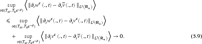
The subsequent calculation uses first a triangle inequality and then the convergence (5.7) for the first term and the convergence (5.5) for the second term:

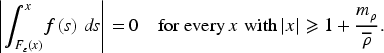
\begin{aligned} sup_{t \in (T_{M}, T_{0} ε^{- β})} ⟨ ‖ \partial_{t} w^{ε} (., t) - \partial_{t} \bar{v} (., t) ‖_{L^{2} (R_{+})} ⟩ \\ ⩽ sup_{t \in (T_{M}, T_{0} ε^{- β})} ⟨ ‖ \partial_{t} w^{ε} (., t) - \partial_{t} v^{ε} (., t) ‖_{L^{2} (R_{+})} ⟩ \\ + sup_{t \in (T_{M}, T_{0} ε^{- β})} ⟨ ‖ \partial_{t} v^{ε} (., t) - \partial_{t} \bar{v} (., t) ‖_{L^{2} (R_{+})} ⟩ \to 0. \end{aligned}

(5.9)

Step 3: Deviation of $w^{ε}$ and $\bar{v}$ . We will now verify that (5.9) leads to a contradiction. We can assume that $\bar{g} \neq 0$ is satisfied, otherwise we switch to $x < 0$ and consider h instead of g. Since $\bar{g}$ has support in $ξ \in [- M, M]$ , the functions $\bar{u} (., t) = \bar{v} (., t)$ and $\partial_{t} \bar{u} (., t) = \partial_{t} \bar{v} (., t)$ have support in $x \in [\bar{a} t - M, \bar{a} t + M]$ .

Fix an arbitrary $T_{1} \in (0, T_{0})$ and consider the sequence of time instances $t := t_{ε} := T_{1} ε^{- β}$ . We claim that there exists an event $Ω_{1} \subset Ω_{P}$ with $P (Ω_{1}) > 0$ , such that

\begin{aligned} supp (\partial_{t} w^{ε} (., t; ω)) \cap [\bar{a} t - M, \bar{a} t + M] = \emptyset \end{aligned}

(5.10)

for every

ω \in Ω_{1}

. Loosely speaking: With a positive probability, the pulse of

w^{ε}

is not approximately moving with speed

\bar{a}

Using the claim, we can conclude the proof: Since the $‖ \partial_{t} \bar{v} (., t) ‖_{L^{2} (R_{+})}$ is a positive quantity for every $t > 1$ , (5.10) yields a contradiction to (5.9). This contradiction implies that (5.1) is true.

Step 4: Verification of the claim. The corresponding calculation was performed before, see (2.18) with the resulting mismatch of arrival times (2.19). When the mismatch exceeds $C M$ for sufficiently large $C > 0$ , then (5.10) holds.

Proof of Part (2) of Theorem 5.1. Proof of Part (2) of Theorem 5.1.

Let f be as in the statement and let $u^{ε}$ and $\bar{u}$ be corresponding solutions. It suffices to show the statement (5.2) with $\partial_{t} u^{ε}$ and $\partial_{t} \bar{u}$ replaced by $u^{ε}$ and $\bar{u}$ . Indeed, since f is smooth and $ρ_{ε}, a_{ε}$ are independent of time, the time derivatives $\partial_{t} u^{ε}$ and $\partial_{t} \bar{u}$ are again solutions for a wave equation with trivial initial data and the result for values can be applied to derivatives.

Step 1: Homogenization for finite time. For every fixed $T_{0} > 0$ , we find $C = C (T_{0}, Λ, f) < \infty$ with

\begin{aligned} sup_{t \in (0, T_{0}]} ⟨ {‖ u^{ε} (\cdot, t) - \bar{u} (\cdot, t) ‖}_{L^{2} (R)}^{2} + {‖ \partial_{t} u^{ε} (\cdot, t) - \partial_{t} \bar{u} (\cdot, t) ‖}_{L^{2} (R)}^{2} ⟩ ⩽ C ε . \end{aligned}

(5.11)

The statement is classical and we display a proof relying on Lemma 3.2 for completeness. Setting $\bar{a} := ⟨ a_{0}^{- 1} ⟩^{- 1}$ and $\bar{ρ} := ⟨ a_{0}^{- 1} ⟩$ , we deduce from $a = ρ^{- 1}$ , the definitions of Φ and $Ψ$ of (2.5), and the scaled correctors $Ψ_{ε} (x) = ε Ψ (x / ε)$ and $Φ_{ε} (x) = ε Φ (x / ε)$ that

\begin{aligned} Ψ (y) = Φ (y) = \int_{0}^{y} \frac{\bar{a}}{a (s)} - 1 d s and Ψ_{ε} (x) = Φ_{ε} (x) = \int_{0}^{x} \frac{\bar{a}}{a_{ε} (ξ)} - 1 d ξ . \end{aligned}

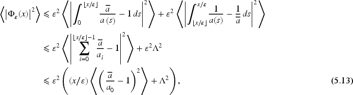
We claim that there exists

C = C (Λ)

such that

\begin{aligned} ⟨ {| Φ_{ε} (x) |}^{2} ⟩ = ⟨ {| Ψ_{ε} (x) |}^{2} ⟩ ⩽ C ε (| x | + ε) . \end{aligned}

(5.12)

In order to show the claim, we consider in the following, without loss of generality, only points

x > 0

. We estimate

\begin{aligned} ⟨ {| Φ_{ε} (x) |}^{2} ⟩ & ⩽ ε^{2} ⟨ {| \int_{0}^{⌊ x / ε ⌋} \frac{\bar{a}}{a (s)} - 1 d s |}^{2} ⟩ + ε^{2} ⟨ {| \int_{⌊ x / ε ⌋}^{x / ε} \frac{1}{a (s)} - \frac{1}{\bar{a}} d s |}^{2} ⟩ \\ ⩽ ε^{2} ⟨ {| \sum_{i = 0}^{⌊ x / ε ⌋ - 1} \frac{\bar{a}}{a_{i}} - 1 |}^{2} ⟩ + ε^{2} Λ^{2} \\ ⩽ ε^{2} ((x / ε) ⟨ {(\frac{\bar{a}}{a_{0}} - 1)}^{2} ⟩ + Λ^{2}), \end{aligned}

(5.13)

where

⌊ p ⌋ := sup {z \in Z | z ⩽ p}

. We used in the last inequality the fact that the

(a_{i})_{i \in Z}

are i.i.d., in particular,

\begin{aligned} \begin{matrix} ⟨ (\frac{\bar{a}}{a_{i}} - 1) (\frac{\bar{a}}{a_{j}} - 1) ⟩ = ⟨ (\frac{\bar{a}}{a_{i}} - 1) ⟩ ⟨ (\frac{\bar{a}}{a_{j}} - 1) ⟩ = 0 \forall i \neq j . \end{matrix} \end{aligned}

This shows the claim, estimate (5.12) for

Φ_{ε}

and, hence, also for

Ψ_{ε}

Inserting (5.12) into (3.13), we obtain

\begin{aligned} \begin{matrix} sup_{t \in [0, T]} ⟨ E_{ε} (t) ⟩ ⩽ C ε, \end{matrix} \end{aligned}

where

C = C (Λ, f, T)

and

E_{ε}

is given in (3.3). Inserting the above estimate and (5.12) into (3.15), we deduce

\begin{aligned} \begin{array}{r} sup_{t \in (0, T_{0}]} ⟨ {‖ \partial_{t} u^{ε} (\cdot, t) - \partial_{t} \bar{u} (\cdot, t) ‖}_{L^{2} (R)}^{2} ⟩ ⩽ C ε \end{array} \end{aligned}

for some

C = C (Λ, T_{0}, f)

. The remaining estimate for

u^{ε} (\cdot, t) - \bar{u} (\cdot, t)

follows by integrating in time, exploiting that

u^{ε}

and

\bar{u}

have trivial initial conditions.

Step 2: Representation formula of solutions for times $t ⩾ 2$ . We use the function $F_{ε} (x) = \int_{0}^{x} a_{ε} {(s)}^{- 1} d s$ , which defines harmonic coordinates (note that we use our particular sign convention for integrals when x is negative). Lemma A.1 allows, for $t ⩾ 2$ , to represent the solutions:

\begin{aligned} u^{ε} (x, t) = \frac{1}{2} (g^{ε} (F_{ε} (x) - (t - 2)) + g^{ε} (F_{ε} (x) + (t - 2))) + \frac{1}{2} \int_{F_{ε} (x) - (t - 2)}^{F_{ε} (x) + (t - 2)} h^{ε} (y) d y, \\ \bar{u} (x, t) = \frac{1}{2} (\bar{g} (\frac{x}{\bar{a}} - (t - 2)) + \bar{g} (\frac{x}{\bar{a}} + (t - 2))) + \frac{1}{2} \int_{\frac{x}{\bar{a}} - t - 2}^{\frac{x}{\bar{a}} + t - 2} \bar{h} (y) d y, \end{aligned}

where

g^{ε}, h^{ε}

and

\bar{g}, \bar{h}

are given by the relations

\begin{aligned} \begin{matrix} u^{ε} (x, 2) = g^{ε} (F_{ε} (x)), \partial_{t} u^{ε} (x, 2) = h^{ε} (F_{ε} (x)) \end{matrix} \end{aligned}

and

\begin{aligned} \begin{matrix} \bar{u} (x, 2) = \bar{g} (\frac{x}{\bar{a}}), \partial_{t} \bar{u} (x, 2) = \bar{h} (\frac{x}{\bar{a}}) . \end{matrix} \end{aligned}

We will later use several properties of the functions

u^{ε}, \bar{u}

and the representing functions

g^{ε}, \bar{g}

and

h^{ε}, \bar{h}

. The smoothness of f implies that there exists

L = L (Λ, f)

such that

\begin{aligned} {‖ \partial_{x} \bar{u} (\cdot, 2) ‖}_{\infty} + {‖ \partial_{x} \partial_{t} \bar{u} (\cdot, 2) ‖}_{\infty} + {‖ \bar{g}^{'} ‖}_{\infty} + {‖ \bar{h}^{'} ‖}_{\infty} ⩽ L . \end{aligned}

(5.14)

Moreover, there exists

M = M (Λ)

such that

\begin{aligned} \forall x \in R ∖ (- M, M) : | \partial_{t} u^{ε} (x, 2) | + | \partial_{t} \bar{u} (x, 2) | + | \partial_{t} \bar{u} (\bar{a} F_{ε} (x), 2) | = 0, \end{aligned}

(5.15)

where we use for the last term on the right-hand side

Λ^{- 1} x ⩽ F_{ε} (x) ⩽ Λ x

Finally, we note that the explicit expressions for $u_{ε}$ and $\bar{u}$ yield for $t ⩾ 2$

\begin{aligned} u^{ε} (x, t) - \bar{u} (x, t) = \frac{1}{2} (I_{ε} (x, t) + {\tilde{I}}_{ε} (x, t)) + \frac{1}{2} J_{ε} (x, t), \end{aligned}

(5.16)

where

\begin{aligned} I_{ε} (x, t) & := g^{ε} (F_{ε} (x) - (t - 2)) - \bar{g} (\frac{x}{\bar{a}} - (t - 2)) \end{aligned}

(5.17)

\begin{aligned} {\tilde{I}}_{ε} (x, t) & := g^{ε} (F_{ε} (x) + (t - 2)) - \bar{g} (\frac{x}{\bar{a}} + (t - 2)) \end{aligned}

(5.18)

\begin{aligned} J_{ε} (x, t) & := \int_{F ε (x) - (t - 2)}^{F ε (s) + (t - 2)} h^{ε} (y) d y - \int_{\frac{x}{\bar{a}} - (t - 2)}^{\frac{x}{\bar{a}} + (t - 2)} \bar{h} (y) d y . \end{aligned}

(5.19)

In the following two steps, we estimate

I_{ε}

and

J_{ε}

separately.

Step 3: Estimates for the error terms $I_{ε}$ and ${\tilde{I}}_{ε}$ . We claim that, for all $T_{0} > 0$ and $β < 1$ , there holds

\begin{aligned} lim_{ε \to 0} sup_{t \in [2, T_{0} ε^{- β}]} ⟨ \int_{R} {| I_{ε} (x, t) |}^{2} d x ⟩ = 0, lim_{ε \to 0} sup_{t \in [2, T_{0} ε^{- β}]} ⟨ \int_{R} {| {\tilde{I}}_{ε} (x, t) |}^{2} d x ⟩ = 0. \end{aligned}

(5.20)

We will show the claim related to

I_{ε}

, the term

{\tilde{I}}_{ε}

can be treated similarly. We use the triangle inequality to split

I_{ε}

into two other terms and write

\begin{aligned} | I_{ε} (x, t) | ⩽ | I_{ε}^{(1)} (x, t) | + | I_{ε}^{(2)} (x, t) | \end{aligned}

(5.21)

with

\begin{aligned} I_{ε}^{(1)} (x, t) & := g^{ε} (F_{ε} (x) - (t - 2)) - \bar{g} (F_{ε} (x) - (t - 2)), \\ I_{ε}^{(2)} (x, t) & := \bar{g} (F_{ε} (x) - (t - 2)) - \bar{g} (\frac{x}{\bar{a}} - (t - 2)) . \end{aligned}

We begin with the term

I_{ε}^{(2)}

. Using that

\bar{g}

has support in

(- M, M)

, the estimates

‖ {\bar{g}}^{'} ‖_{L^{\infty} (R^{d})} ⩽ L < \infty

and

Λ^{- 1} | x | ⩽ | F_{ε} (x) | ⩽ Λ | x |

, we obtain

\begin{aligned} ⟨ \int_{R} {| I_{ε}^{(2)} (x, t) |}^{2} d x ⟩ & ⩽ L^{2} \int_{t - 2 - Λ M}^{t - 2 + Λ M} ⟨ {| F_{ε} (x) - \frac{x}{\bar{a}} |}^{2} ⟩ d x \\ = \frac{L^{2}}{\bar{a}} \int_{t - 2 - Λ M}^{t - 2 + Λ M} ⟨ {| Φ_{ε} (x) |}^{2} ⟩ d x ⩽ C ε (t + 1), \end{aligned}

where we used (5.12) in the last step and a constant

C = C (Λ, f) < \infty

We now estimate the term involving $I_{ε}^{(1)}$ . A change of variables with $y = F_{ε}^{- 1} (F_{ε} (x) - (t - 2))$ and, accordingly, $d y = (F_{ε}^{- 1})^{^{'}} (F_{ε} (x) - (t - 2)) F_{ε}^{^{'}} (x) d x$ with pre-factor $(F_{ε}^{- 1})^{^{'}} (F_{ε} (x) - (t - 2)) F_{ε}^{^{'}} (x) ⩾ Λ^{- 2}$ allows to calculate

\begin{aligned} ⟨ \int_{R} {| I_{ε}^{(1)} (x, t) |}^{2} d x ⟩ & ⩽ Λ^{2} ⟨ \int_{R} {| g^{ε} (F_{ε} (y)) - \bar{g} (F_{ε} (y)) |}^{2} d y ⟩ \\ ⩽ 2 Λ^{2} (⟨ \int_{R} {| u^{ε} (y, 2) - \bar{u} (y, 2) |}^{2} d y ⟩ + ⟨ \int_{R} {| I_{ε}^{(2)} (x, 2) |}^{2} d x ⟩), \end{aligned}

(5.22)

where we use triangle inequality and the definition of

g^{ε}

and

\bar{g}

in the second inequality.

We can now combine (5.22) and (5.11) (with $T_{0} = 2$ ). We obtain, for some $C = C (f, Λ) < \infty$ and arbitrary $t > 2$ :

\begin{aligned} ⟨ \int_{R} | I_{ε} (x, t) |^{2} d x ⟩ ⩽ C ε (1 + t) . \end{aligned}

(5.23)

With this estimate, we have shown the claim of (5.20).

Step 4: Estimate for the error term $J_{ε}$ . We claim that $J_{ε}$ defined in (5.19) satisfies

\begin{aligned} \forall T_{0} > 0, β < 1 : lim_{ε \to 0} sup_{t \in [2, T_{0} ε^{- β}]} ⟨ \int_{R} {| J_{ε} (x, t) |}^{2} d x ⟩ = 0. \end{aligned}

(5.24)

We start the proof by writing

\begin{aligned} \begin{matrix} J_{ε} (x, t) = \sum_{k = 1}^{3} J_{ε}^{(k)} (x, t) \end{matrix} \end{aligned}

with

\begin{aligned} J_{ε}^{(1)} (x, t) & := \int_{F_{ε} (x) - (t - 2)}^{F_{ε} (x) + (t - 2)} h^{ε} (y) - \partial_{t} \bar{u} (F_{ε}^{- 1} (y), 2) d y, \\ J_{ε}^{(2)} (x, t) & := \int_{F_{ε} (x) - (t - 2)}^{F_{ε} (x) + (t - 2)} \partial_{t} \bar{u} (F_{ε}^{- 1} (y), 2) - \partial_{t} \bar{u} (\bar{a} y, 2) d y, \\ J_{ε}^{(3)} (x, t) & := \int_{F_{ε} (x) - (t - 2)}^{F_{ε} (x) + (t - 2)} \partial_{t} \bar{u} (\bar{a} y, 2) d y - \int_{\frac{x}{\bar{a}} - (t - 2)}^{\frac{x}{\bar{a}} + (t - 2)} \bar{h} (y) d y . \end{aligned}

Recalling

h^{ε} (y) = \partial_{t} u^{ε} (z, 2)

for

z = F_{ε}^{- 1} (y)

, we obtain, using the corresponding substitution in the first equality,

\begin{aligned} ⟨ \int_{R} {| J_{ε}^{(1)} (x, t) |}^{2} d x ⟩ & = ⟨ \int_{R} {| \int_{F_{ε}^{- 1} (F_{ε} (x) - (t - 2))}^{F_{ε}^{- 1} (F_{ε} (x) + (t - 2))} (\partial_{t} u^{ε} (z, 2) - \partial_{t} \bar{u} (z, 2)) F_{ε}^{^{'}} (z) d z |}^{2} d x ⟩ \\ \overset{(5.15)}{⩽} Λ^{2} ⟨ \int_{U_{ε} (t)} {| \int_{- M}^{M} | \partial_{t} u^{ε} (z, 2) - \partial_{t} \bar{u} (z, 2) | d z |}^{2} d x ⟩, \end{aligned}

where the outer domain of integration is

\begin{aligned} U_{ε} (t) := {x \in R | (F_{ε}^{- 1} (F_{ε} (x) - (t - 2)), F_{ε}^{- 1} (F_{ε} (x) + (t - 2))) \cap (- M, M) \neq \emptyset} \end{aligned}

and where we used

‖ F_{ε}^{^{'}} ‖_{\infty} ⩽ Λ

Because of $F_{ε} (0) = 0$ and $‖ F_{ε}^{^{'}} ‖_{L^{\infty}}, ‖ (F_{ε}^{- 1})^{^{'}} ‖_{L^{\infty}} ⩽ Λ$ , we obtain $U_{ε} (t) \subset U (t)$ for some deterministic $U (t)$ satisfying $| U (t) | = C (1 + t)$ for some $C = C (Λ)$ . We therefore find $C = C (Λ, f)$ such that, changing the constant from one line to the next,

\begin{aligned} ⟨ \int_{R} {| J_{ε}^{(1)} (x, t) |}^{2} d x ⟩ & ⩽ C (1 + t) ⟨ \int_{R} {| \partial_{t} u^{ε} (z, 2) - \partial_{t} \bar{u} (z, 2) |}^{2} d z ⟩ \\ \overset{(5.11)}{⩽} C (1 + t) ε . \end{aligned}

(5.25)

In order to estimate the term involving $J_{ε}^{(2)}$ , we substitute again $z = F_{ε}^{- 1} (y)$ with $d y = F_{ε}^{^{'}} (z) d z = \frac{1}{a_{ε} (z)} d z$ and obtain

\begin{aligned} ⟨ \int_{R} {| J_{ε}^{(2)} (x, t) |}^{2} d x ⟩ & = ⟨ \int_{R} {| \int_{F_{ε}^{- 1} (F_{ε} (x) - (t - 2))}^{F_{ε}^{- 1} (F_{ε} (x) + (t - 2))} \frac{\partial_{t} \bar{u} (z, 2) - \partial_{t} \bar{u} (\bar{a} F_{ε} (z), 2)}{a_{ε} (z)} d z |}^{2} d x ⟩ \\ \overset{(5.15)}{⩽} Λ^{2} ⟨ \int_{U_{ε} (t)} {| \int_{- M}^{M} | \partial_{t} \bar{u} (z, 2) - \partial_{t} \bar{u} (\bar{a} F_{ε} (z), 2) | d z |}^{2} d x ⟩, \end{aligned}

where

U_{ε} (t) \subset U (t)

with

| U (t) | ⩽ C (1 + t)

are as above. The Cauchy–Schwarz inequality implies

\begin{aligned} ⟨ \int_{R} {| J_{ε}^{(2)} (x, t) |}^{2} d x ⟩ & ⩽ Λ^{2} | U (t) | 2 M ⟨ \int_{- M}^{M} {| \partial_{t} \bar{u} (z, 2) - \partial_{t} \bar{u} (\bar{a} F_{ε} (z), 2) |}^{2} d z ⟩ \\ ⩽ C (1 + t) ‖ \partial_{x} \partial_{t} \bar{u} ‖_{\infty}^{2} \int_{- M}^{M} ⟨ {| z - \bar{a} F_{ε} (z) |}^{2} ⟩ d z, \end{aligned}

where

C = C (Λ)

(recall

M = M (Λ)

). We use the equality

| z - \bar{a} F_{ε} (z) | = | Φ_{ε} (z) |

to conclude from (5.12) and

‖ \partial_{x} \partial_{t} \bar{u} ‖_{\infty} ⩽ C (Λ, f)

, that

\begin{aligned} ⟨ \int_{R} {| J_{ε}^{(2)} (x, t) |}^{2} d x ⟩ ⩽ C (1 + t) ε \end{aligned}

(5.26)

for some

C = C (Λ, f)

. It remains to estimate the term involving

J_{ε}^{(3)}

. We observe that

\partial_{t} \bar{u} (\bar{a} y, 2) = \bar{h} (y)

and thus

\begin{aligned} | J_{ε}^{(3)} (x, t) | ⩽ 2 ‖ h ‖_{\infty} | F_{ε} (x) - \frac{x}{\bar{a}} | = 2 ‖ h ‖_{\infty} | Φ_{ε} (x) | / \bar{a} \end{aligned}

for all

x \in R

. Furthermore,

J_{ε}^{(3)} (x, t) = 0

holds unless

\begin{aligned} (F_{ε} (x) - (t - 2), F_{ε} (x) + (t - 2)) \cap (- M, M) \neq \emptyset or \\ (\frac{x}{\bar{a}} - (t - 2), \frac{x}{\bar{a}} + (t - 2)) \cap (- M, M) \neq \emptyset . \end{aligned}

Arguing similar to the case of

J_{ε}^{(2)}

we deduce with help of (5.12)

\begin{aligned} ⟨ \int_{R} {| J_{ε}^{(3)} (x, t) |}^{2} d x ⟩ ⩽ C (1 + t) ε \end{aligned}

(5.27)

for some

C = C (Λ, f)

. Combining (5.25)–(5.27), we obtain (5.24), and have therefore shown the claim for

J_{ε}

Step 6: Conclusion. The decomposition (5.16) combined with (5.20) and (5.24) imply the claim.

Remark 5.2 (Extensions to correlated coefficients)

Theorem 5.1 can be extended to certain correlated media. Indeed, the fact that the coefficients are i.i.d. is used, in the proof of Theorem 5.1, essentially only for the calculation

\begin{aligned} ε^{2} (| x | / ε - 1) ≲ ⟨ | Φ_{ε} (x) |^{2} ⟩ ≲ ε^{2} (| x | / ε + 1) . \end{aligned}

The upper bound is used in all applications of estimate (5.13) and the lower bound in (2.18) and (2.19) (note that

⟨ Δ_{ε} {(x)}^{2} ⟩ = {\bar{a}}^{2} ⟨ | Φ_{ε} (x) |^{2} ⟩

with

x := ε j

). In Section C below, we construct, for every

γ \in (1 / 2, 1)

a random medium where the corrector satisfies bounds of the form

\begin{aligned} ε^{2 (1 - γ)} (| x |^{2 γ} - 1) ≲ ⟨ | Φ_{ε} (x) |^{2} ⟩ ≲ ε^{2 (1 - γ)} (| x |^{2 γ} + 1) . \end{aligned}

(5.28)

Next, we briefly sketch that the corrector estimates (5.28) yield results that are analogous to those of Theorem 5.1, where the critical time $ε^{- 1}$ is replaced by $ε^{- \frac{1 - γ}{γ}}$ . Indeed, if we replace (5.13) with the upper bound in (5.28), we obtain that (5.23) and (5.25)–(5.27) hold with

\begin{aligned} \begin{matrix} ε (1 + t) replaced by ε^{2 (1 - γ)} (1 + t^{2 γ}) . \end{matrix} \end{aligned}

Clearly, this implies (5.20) and (5.24) with $β < 1$ replaced by $β < \frac{1 - γ}{γ}$ . Similarly, we obtain that the lower bound of (5.28) implies that (2.19) is replaced by

\begin{aligned} | {\bar{T}}_{ε} (x_{ε}) - \bar{T} (x_{ε}) | = | Δ_{ε} (x_{ε}) | ≳ ε^{1 - γ} (1 + ε^{- 2 γ β})^{\frac{1}{2}}, \end{aligned}

and the right-hand side diverges when

β > \frac{1 - γ}{γ}

Footnotes

Representation of matched impedance solutions

We state and prove a d’Alambert-type representation formula for solutions of the initial-value problem with matched impedance. We use this formula in the proof of Theorem 5.1. Lemma A.1.

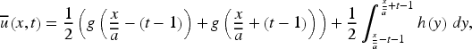
For $Λ ⩾ 1$ , let $a, ρ : R \to [Λ^{- 1}, Λ]$ be coefficients such that $a ρ = 1$ holds almost everywhere. We use the function $F (x) := \int_{0}^{x} (a (s))^{- 1} d s$ (with the standard sign convention for integrals). Then, for arbitrary $g, h \in L^{\infty} (R)$ with compact support, the unique solution u of the wave equation

\begin{aligned} ρ \partial_{t}^{2} u - \partial_{x} (a \partial_{x} u) = 0 with u (\cdot, 0) = g \circ F, \partial_{t} u (\cdot, 0) = h \circ F \end{aligned}

is given by

(A.1)

\begin{aligned} u (x, t) = \frac{1}{2} (g (F (x) - t) + g (F (x) + t)) + \frac{1}{2} \int_{F (x) - t}^{F (x) + t} h (y) d y . \end{aligned}

Proof.

Uniqueness of the solution is known, the attainment of the initial values is easily checked. We only have to show that the expression in (A.1) solves the wave equation. We compute

\begin{aligned} \begin{matrix} \partial_{t}^{2} u (x, t) = \frac{1}{2} (g^{″} (F (x) - t) + g^{″} (F (x) + t) + h^{'} (F (x) + t) - h^{'} (F (x) - t)) . \end{matrix} \end{aligned}

Using

F^{'} (x) = 1 / a (x)

, we obtain for the first spatial derivative of u

\begin{aligned} a (x) \partial_{x} u (x, t) = \frac{1}{2} (g^{'} (F (x) - t) + g^{'} (F (x) + t) + h (F (x) + t) - h (F (x) - t)) . \end{aligned}

Taking another spatial derivative, the chain rule yields

\begin{aligned} \begin{array}{r} \partial_{x} (a (x) \partial_{x} u (x, t)) = \frac{1}{a (x)} \partial_{t}^{2} u (x, t) . \end{array} \end{aligned}

Because of

ρ = 1 / a

, we have found that u solves the wave equation.

A small right hand side in the wave equation

In this section, we formulate and prove a technical lemma which is used in the proof of Proposition 4.5. Lemma B.1.

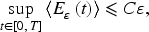
Let $L ⩾ 1$ be a bound for the support of functions. We consider, for every $ε > 0$ , a function $g_{ε} : R \times R_{+} \times Ω_{P} \to R$ such that $g_{ε} (\cdot, ω)$ is supported in $[- L, L] \times [0, L]$ for every $ω \in Ω_{P}$ . We furthermore assume that the quantity $G_{ε} (x, t, ω) := \int_{0}^{x} g_{ε} (s, t, ω) d s$ satisfies

\begin{aligned} lim_{ε \to 0} sup_{t ⩾ 0} \int_{R} ⟨ | G_{ε} (\cdot, t) |^{2} ⟩ + ⟨ | \partial_{t} G_{ε} (\cdot, t) |^{2} ⟩ d x = 0. \end{aligned}

Then, for every

M \in [1, \infty)

and every sequence of coefficients

a_{ε}, ρ_{ε} : R \times Ω_{P} \to R

satisfying

a_{ε}, ρ_{ε} \in [1 / M, M]

for all

ε > 0

, the sequence of solutions

w^{ε}

(B.1)

\begin{aligned} ◻_{ε} w^{ε} := ρ_{ε} \partial_{t}^{2} w^{ε} - \partial_{x} (a_{ε} \partial_{x} w^{ε}) = g_{ε}, w i t h w^{ε} (\cdot, 0) = \partial_{t} w^{ε} (\cdot, 0) = 0 \end{aligned}

satisfies

(B.2)

\begin{aligned} lim_{e ↘ 0} sup_{t ⩾ 0} ⟨ {‖ \partial_{t} w^{ε} (\cdot, t) ‖}_{L^{2} (R)}^{2} ⟩ = 0. \end{aligned}

Proof.

Throughout the proof we denote by $E_{ε} (t)$ the energy of $w^{ε} (\cdot, t)$ that is

\begin{aligned} E_{ε} (t) := \frac{1}{2} \int_{R} ρ_{ε} {| \partial_{t} w^{ε} (\cdot, t) |}^{2} + a_{ε} {| \partial_{x} w^{ε} (\cdot, t) |}^{2} . \end{aligned}

The definition of

G_{ε}

imply that

w^{ε}

solves the equation

\begin{aligned} ◻_{ε} w^{ε} = \partial_{x} G_{ε} . \end{aligned}

Now we can apply the same (standard) testing procedure as in Step 2 of the proof of Lemma 3.1. By multiplying the above equation with

\partial_{t} w^{ε}

and integrating, we obtain (with help of integration by parts)

\begin{aligned} \begin{matrix} E_{ε} (t) = \int_{0}^{t} \int_{R} (\partial_{x} G_{ε}) \partial_{t} w^{ε} = \int_{0}^{t} \int_{R} (\partial_{t} G_{ε}) \partial_{x} w^{ε} - \int_{R} G_{ε} (\cdot, t) \partial_{t} w^{ε} (\cdot, t) . \end{matrix} \end{aligned}

As in Step 2 of the proof of Lemma 3.1, we deduce from the above identity that

\begin{aligned} sup_{t \in [0, T]} ⟨ E_{ε} (t) ⟩ ⩽ C T \int_{0}^{T} \int_{R} ⟨ {| \partial_{t} G_{ε} |}^{2} ⟩ + C sup_{t \in [0, T]} \int_{R} ⟨ {| G_{ε} (\cdot, t) |}^{2} ⟩, \end{aligned}

where

C = C (M) > 0

. Recall that

g_{ε}

and thus

G_{ε}

is supported in time in

[0, L]

and thus we obtain by sending

T \to \infty

\begin{aligned} sup_{t ⩾ 0} E_{ε} (t) ⩽ C (L^{2} + 1) sup_{t ⩾ 0} (\int_{R} ⟨ {| \partial_{t} G_{ε} (\cdot, t) |}^{2} ⟩ + ⟨ {| G_{ε} (\cdot, t) |}^{2} ⟩ d x \to 0 as ε \to 0. \end{aligned}

which completes the proof.

Media with γ ∈ ( 1 / 2,1 )

Our standard random medium has identically distributed independent values of ρ and a, which results in a model parameter $γ = \frac{1}{2}$ (growth of correctors). When the values of ρ (or a) are not independent in the different cells, but have a positive correlation, then every value of γ in the interval $(\frac{1}{2}, 1)$ can occur. This is what we show in this section with a construction from [6].

For simplicity, we consider media with constant ρ, say $ρ \equiv 1$ , and random a. An extension to more general models, in particular models $(a, ρ)$ of class $γ \in (\frac{1}{2}, 1)$ with matched impedance ( $ρ a \equiv 1$ ) is straightforward. Let us emphasize that the following construction and computations are essentially contained in [6], where precise $1 D$ elliptic homogenization results in correlated media are proven.

For a given probability space $(Ω_{P}, A, P)$ let ${g (x) | x \in R}$ be a stationary Gaussian process. We suppose that, for every $x \in R$ , the random variable $g (x, \cdot) : Ω_{P} \to R$ has zero mean and variance one, $⟨ g (x) ⟩ = 0$ and $⟨ g {(x)}^{2} ⟩ = 1$ for every x. Moreover, we suppose that the autocorrelation function

\begin{aligned} R_{g} (t) := ⟨ g (x) g (x + t) ⟩ \end{aligned}

satisfies, for some exponent

α \in (0, 1)

and some factor

κ_{g} > 0

, (C.1)

\begin{aligned} R_{g} (t) \sim κ_{g} t^{- α} as t \to \infty, which is defined as: lim_{t \to \infty} t^{α} R_{g} (t) = κ_{g} . \end{aligned}

Our aim is to define coefficients

a : R \times Ω_{P} \to R

that satisfy uniform bounds. We will define them by truncating the Gaussian variable

g (x)

. We fix a nonlinear map

T : R \to R

satisfying

| T (x) | ⩽ \frac{1}{2}

and

T (x) = - T (- x)

for all

x \in R

. Possible choices are

T = \frac{1}{2} sgn

T = \frac{1}{4} \arctan

. We consider the random field

\begin{aligned} \begin{matrix} φ (x, ω) := T (g (x, ω)) . \end{matrix} \end{aligned}

The following properties of φ are proven in [6, Proposition 2.2]:

We are now in a position to construct, for every $γ \in (\frac{1}{2}, 1)$ , a model of class γ. Corollary C.2.

Let γ be a number in the interval $(\frac{1}{2}, 1)$ . We choose the parameter $α := 2 (1 - γ) \in (0, 1)$ and consider g and φ as in Lemma C.1. Then $(ρ, a)$ with $ρ \equiv 1$ and $a : R \times Ω_{P} \to R$ given by

\begin{aligned} a (x, ω) := \frac{1}{1 + φ (x, ω)} \end{aligned}

defines a model of class γ.

Proof.

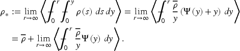
By construction, we have $| φ | ⩽ \frac{1}{2}$ and thus $\frac{2}{3} ⩽ a ⩽ 2$ on $R \times Ω_{P}$ . Moreover, we have

\begin{aligned} ⟨ \frac{1}{a (x)} ⟩ = 1 + ⟨ φ (x) ⟩ = 1, \end{aligned}

and thus

\bar{a} = 1

, see (2.1). Accordingly, the corrector Φ of (2.5) is given by

\begin{aligned} Φ (y) = \int_{0}^{y} {\frac{\bar{a}}{a (s)} - 1} d s = \int_{0}^{y} φ (s) d s . \end{aligned}

The choice

ρ \equiv 1

yields

\bar{ρ} = 1

and

Ψ \equiv 0

. In order to show that

(a, ρ)

defines a model of class

γ = 1 - \frac{α}{2}

it suffices to show the following two statements (compare (2.7)): (C.3)

\begin{aligned} \forall γ^{'} > 1 - \frac{α}{2} : \underset{r \to \infty}{lim sup} \frac{1}{r^{2 γ^{'}}} ⟨ - \int_{0}^{r} {| Φ (y) |}^{2} d y ⟩ = 0 \end{aligned}

and (C.4)

\begin{aligned} \forall γ^{'} < 1 - \frac{α}{2} : \underset{r \to \infty}{lim inf} \frac{1}{r^{2 γ^{'}}} ⟨ - \int_{0}^{r} {| Φ (y) |}^{2} d y ⟩ = + \infty . \end{aligned}

We show (C.3), the computations for (C.4) are similar. As a preparation, we rewrite a double integral with the substitution rule:

\begin{aligned} \int_{0}^{y} \int_{0}^{y} φ (s) φ (t) d t d s & = \int_{0}^{y} \int_{s}^{y} φ (s) φ (t) d t d s + \int_{0}^{y} \int_{0}^{s} φ (s) φ (t) d t d s \\ = \int_{0}^{y} \int_{0}^{y - s} φ (s) φ (s + τ) d τ d s + \int_{0}^{y} \int_{0}^{y - t} φ (t + τ) φ (t) d τ d t \\ = 2 \int_{0}^{y} \int_{0}^{y - s} φ (s) φ (s + τ) d τ d s . \end{aligned}

Using this formula and the autocorrelation function

R (τ) := ⟨ φ (s) φ (s + τ) ⟩

, we find

\begin{aligned} ⟨ - \int_{0}^{r} {| Φ (y) |}^{2} d y ⟩ & = ⟨ - \int_{0}^{r} {| \int_{0}^{y} φ (s) d s |}^{2} d y ⟩ = ⟨ - \int_{0}^{r} \int_{0}^{y} \int_{0}^{y} φ (s) φ (t) d t d s d y ⟩ \\ = 2 - \int_{0}^{r} \int_{0}^{y} \int_{0}^{y - t} R (τ) d τ d t d y . \end{aligned}

Combining (C.2) and

| R (τ) | = | ⟨ φ (x) φ (x + τ) ⟩ | ⩽ \frac{1}{4}

(which follows from

| φ | ⩽ \frac{1}{2}

), we obtain the existence of a constant

C > 0

such that

R ⩽ C

[0, 1]

and

| R (τ) | ⩽ C τ^{- α}

[1, \infty)

. This allows to calculate the expression of (C.3):

\begin{aligned} \frac{1}{r^{2 γ^{'}}} ⟨ - \int_{0}^{r} {| Φ (y) |}^{2} d y ⟩ & = \frac{2}{r^{2 γ^{'}}} - \int_{0}^{r} \int_{0}^{y} \int_{0}^{y - t} R (τ) d τ d t d y \\ ⩽ \frac{2 C}{r^{2 γ^{'}}} - \int_{0}^{r} \int_{0}^{y} (\int_{0}^{min {y - t, 1}} d τ + \int_{min {y - t, 1}}^{y - t} τ^{- α} d τ) d t d y \\ ⩽ \frac{2 C}{r^{2 γ^{'}}} - \int_{0}^{r} \int_{0}^{y} 1 + \frac{(y - t)^{1 - α}}{1 - α} d t d y \\ = \frac{2 C}{r^{2 γ^{'}}} - \int_{0}^{r} y + \frac{1}{(1 - α) (2 - α)} y^{2 - α} d y \\ ⩽ \frac{2 C}{r^{2 γ^{'}}} (r + \frac{1}{(1 - α) (2 - α)} r^{2 - α}) . \end{aligned}

This implies (C.3) because of

2 γ^{'} > 2 - α > 1

As noted above, the computations for (C.4) are analogous. This shows that the model class is indeed γ.

Acknowledgements

This work was partially funded by Deutsche Forschungsgemeinschaft (DFG, German Research Foundation) under grant SCHW 639/11-1, “Strahlungsbedingungen für Wellen in periodischen und stochastischen Medien”.

References

Abdulle

Pouchon

, Effective models and numerical homogenization for wave propagation in heterogeneous media on arbitrary timescales, Found. Comput. Math. 20(6) (2020), 1505–1547. doi:10.1007/s10208-020-09456-x.

Allaire

Briane

Vanninathan

, A comparison between two-scale asymptotic expansions and Bloch wave expansions for the homogenization of periodic structures, SeMA J. 73(3) (2016), 237–259. doi:10.1007/s40324-016-0067-z.

Allaire

Lamacz-Keymling

Rauch

, Crime pays; homogenized wave equations for long times, Asymptot. Anal. 128(3) (2022), 295–336.

Allaire

Yamada

, Optimization of dispersive coefficients in the homogenization of the wave equation in periodic structures, Numer. Math. 140(2) (2018), 265–326. doi:10.1007/s00211-018-0972-4.

Armstrong

Kuusi

Mourrat

J.-C.

, Quantitative Stochastic Homogenization and Large-Scale Regularity, Grundlehren der Mathematischen Wissenschaften [Fundamental Principles of Mathematical Sciences], Vol. 352, Springer, Cham, 2019.

Bal

Garnier

Motsch

Perrier

, Random integrals and correctors in homogenization, Asymptot. Anal. 59(1–2) (2008), 1–26.

Benoit

Gloria

, Long-time homogenization and asymptotic ballistic transport of classical waves, Ann. Sci. Éc. Norm. Supér. (4) 52(3) (2019), 703–759. doi:10.24033/asens.2395.

Blanc

Le Bris

, Homogenization Theory for Multiscale Problems, MS&A Vol. 21, Springer, Cham, 2023.

Brahim-Otsmane

Francfort

G.A.

Murat

, Correctors for the homogenization of the wave and heat equations, J. Math. Pures Appl. (9) 71(3) (1992), 197–231.

10.

Dohnal

Lamacz

Schweizer

, Bloch-wave homogenization on large time scales and dispersive effective wave equations, Multiscale Model. Simul. 12(2) (2014), 488–513. doi:10.1137/130935033.

11.

Dohnal

Lamacz

Schweizer

, Dispersive homogenized models and coefficient formulas for waves in general periodic media, Asymptot. Anal. 93(1–2) (2015), 21–49.

12.

Duerinckx

Gloria

Ruf

, A spectral ansatz for the long-time homogenization of the wave equation, 2023.

13.

Fish

Chen

, Space-time multiscale model for wave propagation in heterogeneous media, Comput. Methods Appl. Mech. Engrg. 193(45–47) (2004), 4837–4856. doi:10.1016/j.cma.2004.05.006.

14.

Fouque

J.-P.

Garnier

Papanicolaou

Sølna

, Wave Propagation and Time Reversal in Randomly Layered Media, Stochastic Modelling and Applied Probability, Vol. 56, Springer, New York, 2007.

15.

Gloria

Neukamm

Otto

, Quantitative estimates in stochastic homogenization for correlated coefficient fields, Anal. PDE 14(8) (2021), 2497–2537. doi:10.2140/apde.2021.14.2497.

16.

Lamacz

, Dispersive effective models for waves in heterogeneous media, Math. Models Methods Appl. Sci. 21(9) (2011), 1871–1899. doi:10.1142/S021820251100557X.

17.

Neukamm

Varga

Waurick

, Two-scale homogenization of abstract linear time-dependent PDEs, Asymptot. Anal. 125(3–4) (2021), 247–287.

18.

Santosa

Symes

W.W.

, A dispersive effective medium for wave propagation in periodic composites, SIAM J. Appl. Math. 51(4) (1991), 984–1005. doi:10.1137/0151049.

19.

Schäffner

Schweizer

Tjandrawidjaja

, Domain truncation methods for the wave equation in a homogenization limit, Appl. Anal. 101(12) (2022), 4149–4170. doi:10.1080/00036811.2022.2054416.

20.

Schweizer

Theil

, Lattice dynamics on large time scales and dispersive effective equations, SIAM J. Appl. Math. 78(6) (2018), 3060–3086. doi:10.1137/17M1162184.