
Abstract
We obtain new results about the high-energy distribution of resonances for the one-dimensional Schrödinger operator. Our primary result is an upper bound on the density of resonances above any logarithmic curve in terms of the singular support of the potential. We also prove results about the distribution of resonances in sectors away from the real axis, and construct a class of potentials producing multiple sequences of resonances along distinct logarithmic curves, explicitly calculating the asymptotic location of these resonances. The results are unified by the use of an integral representation of the reflection coefficients, refining methods used in (J. Differential Equations
Introduction
Main Results
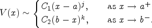
This paper studies relationships between the singularities of a potential
For

Let


The upper bound obtained in the first part of this theorem is optimal (when considered to hold for any value of M). This can be seen from the results of [21, Theorem 6] for a class of potentials V for which
We give a proof of Theorem 1.1 using a Jensen-type formula for ellipses rather than circles, and an upper bound on the determinant of the scattering matrix in appropriate regions of
Before stating further results, we introduce some notation which we shall use throughout the paper. We continue to use
We define a class of potentials of a type considered in [21, Theorem 6] (see also [16] and [18]) although here we allow the potentials to be complex-valued.
We say that For some constants
Zworski shows that real-valued potentials in

Let

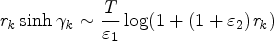
The sequence in this theorem lies approximately on the logarithmic curve


We note that [18] extends [21, Theorem 6] to complex-valued potentials supported in
In Section 3.3 we show that one can choose certain
We now turn to resonances in sectors away from the real axis. For

This next result gives new information about high-energy resonances in sectors away from


Let

Theorem 5.1 shows even more specifically that the resonances of V in this kind of sector
As for so many results in the study of resonances, we reduce the problem to the study of the zeros of an analytic function. We will use both
Section 3.2 proves three extensions of [21, Theorem 6] (see also [18]), including Theorem 1.2. Each of these expands the class of potentials for which one can explicitly calculate (up to small error) a sequence of resonances asymptotic to a logarithmic curve. Section 3.3 also produces examples of such potentials, though we find more complicated behavior as well. For potentials of the type considered in Theorem 1.2, (2.7) allows us to find the leading terms of
Our results in Section 3 give a variety of explicit examples of resonances generated by diffraction of singularities in the homogenous (nonsemiclassical) setting. Theorem 1.2 in particular can be used to give more general examples of the optimality of the resonance-free region for diffractive trapping obtained in [9, Theorem 1] (see [9, Theorem 2] where a potential in
It is a result of Vainberg and Lax-Phillips [14,20] (which holds in more general settings, see also [6, Section 4.6]) that if
We prove Theorem 1.3 in Section 5. Although all of the results of this paper use an intermediate step of [7] (see also [17]) as a starting point, it is the proof of Theorem 1.3 which has the most in common with [7], using results from the theory of entire functions of exponential type.
An appendix provides some applications of a well-known method of G.H. Hardy on locating the solutions of certain transcendental equations which we use repeatedly in Section 3.
In addition to the papers previously mentioned, [12,13] and references therein prove further estimates on resonances in one dimension.
The authors have no competing interests.
Preliminaries
For
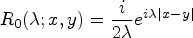
It is well-known (see [6, Chapter 2] and [7]) that resonances can also be identified as the zeros of the Fredholm determinant,

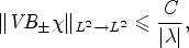
The function
There are constants
In [15, Chapter 16], entire functions satisfying (ii) and the last part of (iii) are said to be of Class C. Applying [15, Section 16.1, Theorem 2] to
Given

Although the exceptional disks in the set
Next we define


We will sometimes use superscripts

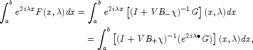
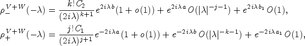
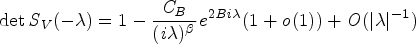
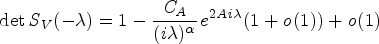
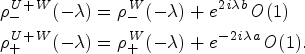
The point of the definitions above is that the following representation of the scattering matrix holds:

We therefore obtain the following useful expansion for the determinant of the scattering matrix:

We note that although it is standard to work with potentials
The definition of


Another tool we will need is the following important property of
Let
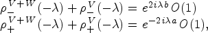
From (2.4) we may write


We need to show that


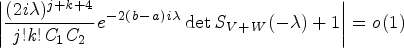
Lemma 2.2 is used in Section 5 through the following corollary giving a bound on the difference of two scattering determinants. Let V and W be as in Lemma 2.2. If Using (2.7) we have


In this section we outline a method which shows how functions in the class
Preliminary Results for
We begin here by developing the tools which allow us to relate the asymptotics of the determinant of the scattering matrix to certain properties of the potential. The potentials we consider in this section consist of sums of functions in
If U is smooth across
Moreover, if
We note that we have not required these functions to have compact support, as we will also use the definition to describe the regularity properties of the functions
We shall see that for some such U, Lemma 3.2 combined with (2.7) shows that the leading behavior of
Let
For
For
For
That To complete the proof of (ii), when The last part of (iii) is obtained from (i) and (ii) in analogous fashion; this completes the proof of the lemma.
For
The proofs of these expansions are very similar, with our lopsided assumptions on U making the one for The definition of


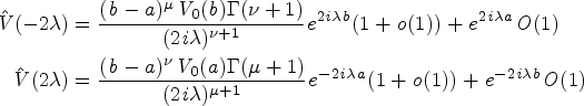
Here we give three extensions of [21, Theorem 6], including Theorem 1.2. Each of these extends the class of potentials for which one can explicitly calculate a sequence of resonances asymptotic to a logarithmic curve.
We first note that the Fourier transform of

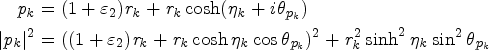
Without loss of generality we assume
With these agreements, we see that


Theorem 1.2 shows that the asymptotic behavior of the sequence of resonances produced by
Let


Let


Next we define

We note that the first part of Theorem 3.3 improves modestly upon Theorem 1.3 for this class of potentials. Examples of W which do not satisfy the support condition and for which the conclusion of the theorem is then false may be constructed using the methods of the next subsection. Indeed, taking

We now show how our method can be used to extend the main result of [18]. There the authors directly analyze certain solutions to

Let V be of the form (3.6) with

We first note that
Using the definitions of


We mention here that we could easily give versions of Theorems 1.2 and 3.3 for V as in Theorem 3.4 and it is interesting to notice what happens to the support condition on W in Theorem 3.3 as
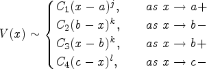
This section contains another extension of [21, Theorem 6]. We will determine the asymptotic distribution of resonances for a potential V which satisfies the following conditions.
Let
We note that
Here we will see that there are three cases, determined by the relative size of three quantities determined by a, b, and c and by j, k, and l. Our results are very similar to the case of the three delta functions potential of [4].
Clearly


(

It is easy to check that the assumption

In

Notice that in Case 1 we obtain asymptotically the same sequence as is given by Theorem 1.2 if there were no singularity at b. The sequence lies approximately on
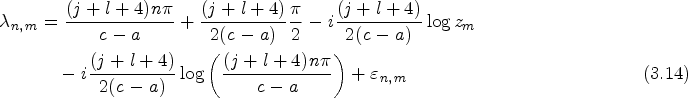
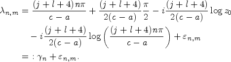
Let V satisfy the hypotheses 3.5, and suppose


The assumption
In

We note the sequence (3.12) lies approximately on
If V satisfies hypotheses 3.5 and
When
In contrast with Case 2, these sequences lie approximately on logarithmic curves which differ at most by a finite shift. Notice moreover that the linear density of each sequence
We also note that the
In this section we prove Theorem 1.1. In order to do so, we first recall a complex analysis result for estimating the number of zeros of an analytic function in an ellipse. The following is taken from [11, Ch. IX, Sec. C, Corollary, pg. 61].
[11].
Let a and

If

The result stated in [11] is actually slightly weaker than this, but the statement above is implied without any change to the proof. We will apply this result to
Let

If
From Section 2, we know that for some

Now, Lemma 2.2 (applied with
Using Lemma 3.2 for the terms


Given


Since in the decomposition (4.3)

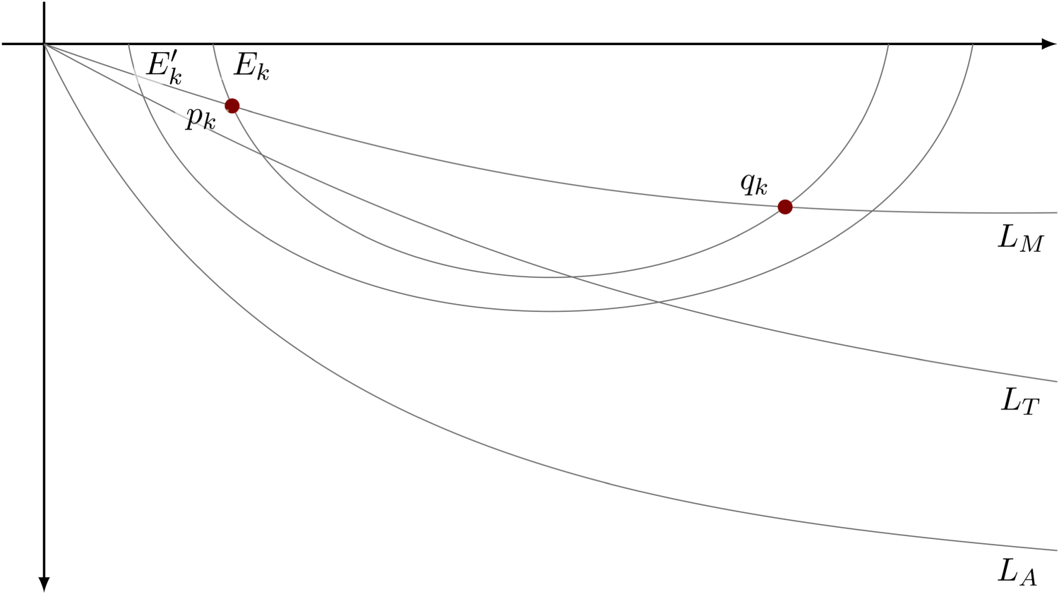
Let
It suffices to prove the claim for Fix the positive constants Curves in the proof of Theorem 4.3. Given M, ellipses As Next we need to show that for a large enough A, the ellipse
In order to produce a contradiction and conclude the proof, we now apply Lemma 4.1 to see that for all k


The idea behind the proof of Theorem 1.3 is to use the lower bound given by Lemma 2.1 and the upper bound given by Lemma 2.3 to produce the inequality

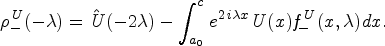
Proof of Theorem 1.3.
From Lemma 2.3 there is an


Since the angles
Next define


We now give a complementary result which follows immediately and shows that, in addition to their counting functions having the same asymptotics, in sectors away from the real axis resonances of the operator
Let

We follow the proof of Theorem 1.3 to obtain (5.3) (which made no assumption that
Footnotes
Applications of Hardy’s method
In this appendix we apply a method of G.H. Hardy which provides a process for asymptotically locating the solutions of certain transcendental equations wherein one first finds preliminary expressions for the possible asymptotic location of solutions, and subsequently proves that such points actually are solutions, by applying Rouché’s theorem.
The method was originally used in [10, Sections 26 and 27] to locate zeros of a particular entire function, and was subsequently applied repeatedly in [2] to study zeros of Fourier transforms of certain classes of functions. More recently, Hardy’s method has been applied to study the distribution of resonances for a compactly supported potential in one dimension [21, Lemma 5], [18, Section 5], for radial potentials in higher odd dimensions [22, Lemma 6], [5, Section 4], and for sums of δ-function potentials [4, Theorem 1].
Here we focus on just two situations for which we have applications in Section 3. The first (Lemma A.1) was referenced previously in [21] but we give an explicit proof here as this version is used repeatedly in this paper. In Lemma A.2 we give an extension which applies to a more complicated case. In both situations, the transcendental equations to which we apply Hardy’s method arise from looking for zeros of analytic functions of a certain form. For
We now give an extension, determining the zeros of a function f having the more complicated form
The first part of the proof of Lemma A.1 follows directly from (A.1)– any large zero must be a point of the sequence (A.2). The proof subsequently shows that these points actually are zeros. In contrast, the added complexity in (A.7) prevents us from concluding that in Lemma A.2 we have found all of the zeros; however, for the application to resonance distribution in Section 3, using the known asymptotics of the resonance counting function, we are able to conclude that we miss at most a set of resonances with linear density zero.