Asymptotic analysis of two-dimensional Oldroyd fluids in unbounded domains: Global attractors and their dimension

Abstract

In this work, we consider the two-dimensional Oldroyd model for the non-Newtonian fluid flows (viscoelastic fluid) in Poincaré domains (bounded or unbounded) and study their asymptotic behavior. We establish the existence of a global attractor in Poincaré domains using asymptotic compactness property. Since the high regularity of solutions is not easy to establish, we prove the asymptotic compactness of the solution operator by applying Kuratowski’s measure of noncompactness, which relies on uniform-tail estimates and the flattening property of the solution. Finally, the estimates for the Hausdorff as well as fractal dimensions of global attractors are also obtained.

Keywords

Oldroyd fluids Global attractors Kuratowski’s measure of noncompactness uniform-tail estimates flattening property fractal and Hausdorff dimensions

1. Introduction

1.1. The model

In this paper, we consider the following hypothesis on the domain Ω:

Hypothesis 1.1.
Let Ω be an open and connected subset of $R^{2}$ , the boundary of which is uniformly of class $C^{3}$ (see [ 18 ]). In addition, there exists a positive constant λ such that the following Poincaré inequality holds:
$\begin{aligned} λ \int_{Ω} {| ψ (x) |}^{2} d x ⩽ \int_{Ω} {| \nabla ψ (x) |}^{2} d x, f o r a l l ψ \in H_{0}^{1} (Ω) . \end{aligned}$
(1.1)
Example 1.2.

If Ω is bounded, then (1.1) is satisfied.

A typical example of unbounded Poincaré domains in $R^{2}$ is $Ω = R \times (- L, L)$ with $L > 0$ , see [48, p.306] and [40, p.117].

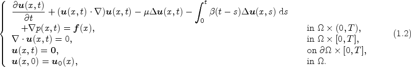
Let us denote by $u (x, t) : Ω \times [0, T] \to R^{2}$ , the velocity of the fluid, $p (x, t) : Ω \times [0, T] \to R$ , the pressure of the fluid and $f (x) : Ω \to R^{2}$ , an external forcing. We consider the following system of equations of motion arising in the Oldroyd fluids of order one for the viscoelastic fluid flows:
$\begin{aligned} {\begin{cases} \frac{\partial u (x, t)}{\partial t} + (u (x, t) \cdot \nabla) u (x, t) - μ Δ u (x, t) - \int_{0}^{t} β (t - s) Δ u (x, s) d s \\ + \nabla p (x, t) = f (x), & in Ω \times (0, T), \\ \nabla \cdot u (x, t) = 0, & in Ω \times [0, T], \\ u (x, t) = 0, & on \partial Ω \times [0, T], \\ u (x, 0) = u_{0} (x), & in Ω . \end{cases} \end{aligned}$
(1.2)
One can impose the condition $\int_{Ω} p (t, x) d x = 0$ , $for~ t ⩾ 0$ , to ensure the uniqueness of pressure p. Let $ν > 0$ be the coefficient of kinematic viscosity. In (1.2), for $\tilde{λ}, κ > 0$ , we take
$\begin{aligned} μ = \frac{κ}{\tilde{λ}} > 0, the kernel β (t) = γ e^{- δ t}, where γ = \frac{1}{\tilde{λ}} (ν - \frac{κ}{\tilde{λ}}) > 0 and δ = \frac{1}{\tilde{λ}} > 0. \end{aligned}$
(1.3)
If we take $ν = \frac{κ}{\tilde{λ}} = μ$ (that is, $γ = 0$ ), then we obtain Newton’s model of incompressible viscous fluid or the well known Navier–Stokes equations. The relaxation time $\tilde{λ}$ is characterized by the fact that after instantaneous cessation of motion, the stresses in the fluid do not vanish instantaneously, but die out like $e^{- {\tilde{λ}}^{- 1} t}$ . Moreover, the velocities of the flow, after instantaneous removal of the stresses, die out like $e^{- κ^{- 1} t}$ , where κ is the retardation time. Note that the system (1.2) is non-autonomous even if the external forcing is independent of t, due to the presence of memory. As the system (1.2) is non-autonomous, in order to apply the asymptotic theory available for the autonomous systems, we need to transform the system (1.2) into an equivalent autonomous system. If we introduce
$\begin{aligned} v (t) := \int_{0}^{t} e^{- δ (t - s)} u (s) d s, \end{aligned}$
(1.4)
then one can rewrite the system (1.2) as
$\begin{aligned} {\begin{cases} \frac{\partial u (x, t)}{\partial t} + (u (x, t) \cdot \nabla) u (x, t) - μ Δ u (x, t) - γ Δ v (x, t) \\ + \nabla p (x, t) = f (x), & in Ω \times (0, T), \\ \frac{\partial v (x, t)}{\partial t} - u (x, t) + δ v (x, t) = 0, & in Ω \times (0, T), \\ \nabla \cdot u (x, t) = 0, & in Ω \times [0, T], \\ u (x, 0) = u_{0} (x), v (x, 0) = 0, & in Ω . \end{cases} \end{aligned}$
(1.5)
1.2. Literature survey

The mathematical analysis of the 2D Oldroyd system (1.2) started with Kotsiolis and Oskolkov [26,37] based on the solvability results available for the Navier–Stokes equations due to Ladyzhenskaya (see [30]). Oskolkov established the global existence of a unique “almost” classical solution in a finite time interval for the initial and boundary value problem for such systems. The questions regarding the existence, uniqueness and continuous dependence of the solutions upon the initial data were investigated by many authors, for instance, see [3–5,9,10,36,37], etc.

For an extensive literature on the existence of global attractors for 2D Navier–Stokes equations, the interested readers are referred to see [1,2,6–8,13–15,17,19,31,41,42,45,48] etc., and references therein. The works [12,16,35,38,43,44,49], etc. discuss attractors and stability for abstract equations and viscoelastic equations with memory. Asymptotic analysis of Navier–Stokes equations with delays has been carried out in [11,33], etc., and references therein. The existence of the global attractor and estimates for its dimensions for the initial-boundary value problem (1.2) with $f \in L^{2} (Ω)$ in a bounded domain with smooth boundary is obtained in [20–23,26–28], etc., using the method developed by Ladyzhenskaya in [31]. Attractor theory of the initial-boundary value problems for equation of motion of Jeffreys–Oldroyd fluids in domains with smooth and nonsmooth boundary is developed in [25].

1.3. Difficulties and approaches

It appears that the transformation provided in (1.4), which transforms the system (1.2) into the autonomous one (1.5), is ineffective. The problem is that, in order for the autonomous attractor theory to work, a semigroup $S (t)$ (solution operator) must map from a phase space into itself; in other words, the phase space as a whole must include the permitted space of initial data. In this case, the allowable initial data is the space $H \times {0}$ , the evolution under the flow will produce a solution that no longer lies in the space $H \times {0}$ . Therefore, we consider the phase space for the initial data as $H \times V$ and show the existence of global attractors for the system (3.2) below. This will imply the existence of global attractors for the system (1.5) (or (3.1) below).

In most of these works mentioned above, the authors applied the theory of global attractors for the system (1.2) (non-autonomous) rather than (1.5) (autonomous), which is not applicable due to the presence of memory term. In this work, we show the existence of global attractors in Poincaré domains for the system (1.5) and obtain estimates for the Hausdorff and fractal dimensions of such attractors. Since the high regularity of solutions for the system (1.5) is not easy establish, we demonstrate the asymptotic compactness of the solution operator by an application of Kuratowski’s measure of noncompactness, which relies on uniform-tail estimates and flattening property of the solution.

1.4. Organization of the paper

The rest of the paper is organized as follows: In the next section, we provide necessary function spaces needed to explain the global solvability results for the system (1.2). As the system (1.2) is non-autonomous due to the presence of memory, using the transformation (1.4), we change the system (1.2) into (1.5), which is autonomous. In Section 3, for $f \in L^{2} (Ω)$ , we show that the system (1.5) in Poincaré domains possesses a global attractor, using asymptotic compactness property of the solution operator (Theorem 3.8). Finally, the estimates for the Hausdorff as well as fractal dimensions of the global attractor for the system (1.5) in Poincaré domains is obtained in Section 4 (Theorem 4.2).

2. Mathematical formulation

In this section, we provide the necessary function spaces needed to obtain the global solvability results of the system (1.2) (equivalently (1.5)). We also discuss the well-posedness of the system (1.2).

2.1. Functional setting

Let $L^{2} (Ω) = L^{2} (Ω; R^{2})$ be the equivalence class of all real valued square integrable functions on $R^{2}$ with the norm defined by $‖ u ‖_{L^{2} (Ω)}^{2} := \int_{Ω} | u (x) |^{2} d x$ . Let $H^{1} (Ω) := H^{1} (Ω; R^{2})$ denotes the Sobolev space $W^{1, 2} (Ω) := W^{1, 2} (Ω; R^{2})$ with the norm defined by $‖ u ‖_{H^{1} (Ω)}^{2} := ‖ u ‖_{L^{2} (Ω)}^{2} + ‖ \nabla u ‖_{L^{2} (Ω)}^{2}$ , $for all u \in H^{1} (Ω)$ . We define the space

\begin{aligned} V := {u \in C_{0}^{\infty} (Ω; R^{2}) : \nabla \cdot u = 0}, \end{aligned}

where

C_{0}^{\infty} (Ω; R^{2})

is the space of all infinitely differentiable functions with compact support in Ω. Let

H

and

V

denote the completion of

V

L^{2} (Ω; R^{2})

and

H^{1} (Ω; R^{2})

norms, respectively. The norm in

H

is defined by

‖ u ‖_{H}^{2} := \int_{Ω} | u (x) |^{2} d x

, and the norm in

V

is given by

‖ u ‖_{V}^{2} := \int_{Ω} | \nabla u (x) |^{2} d x

due to the Poincaré inequality (1.1). The inner product in the Hilbert space

H

is denoted by

(\cdot, \cdot)

and the induced duality between the spaces

V

and its dual

V^{'}

⟨ \cdot, \cdot ⟩

. Note that

V

is densely and continuously embedded into

H

and

H

can be identified with its dual

H^{'}

and we have the Gelfand triple:

V \subset H \equiv H^{'} \subset V^{'}

. In the rest of the paper, we also use the notation

H^{2} (Ω) := H^{2} (Ω; R^{2})

for the second order Sobolev spaces.

2.2. Linear operator

Let $P_{H} : L^{2} (Ω) \to H$ be the Helmholtz–Hodge orthogonal projection. Let us define

\begin{aligned} A u := - P_{H} Δ u, u \in D (A) := V \cap H^{2} (Ω) . \end{aligned}

Remember that the operator A is a non-negative, self-adjoint operator in

H

and

\begin{aligned} ⟨ A u, u ⟩ = ‖ u ‖_{V}^{2}, for all u \in V, so that ‖ A u ‖_{V^{'}} ⩽ ‖ u ‖_{V} . \end{aligned}

(2.1)

2.3. Nonlinear operator

We define the trilinear form $b (\cdot, \cdot, \cdot) : V \times V \times V \to R$ by

\begin{aligned} b (u, v, w) = \int_{Ω} (u (x) \cdot \nabla) v (x) \cdot w (x) d x = \sum_{i, j = 1}^{2} \int_{Ω} u_{i} (x) \frac{\partial v_{j} (x)}{\partial x_{i}} w_{j} (x) d x . \end{aligned}

u

v

are such that the linear map

b (u, v, \cdot)

is continuous on

V

, the corresponding element of

V^{'}

is denoted by

B (u, v)

. We denote

B (u) = B (u, u) = P_{H} [(u \cdot \nabla) u]

. Using integration by parts, it is immediate that

\begin{aligned} {\begin{cases} b (u, v, v) = 0, & for all u, v \in V, \\ b (u, v, w) = - b (u, w, v), & for all u, v, w \in V . \end{cases} \end{aligned}

(2.2)

By an application of Hölder’s and Ladyzhenskaya’s inequalities ([30, Lemma 1, p. 8]), it can be easily seen that B maps

L^{4} (Ω) \cap H

(and so

V

) into

V^{'}

\begin{aligned} | ⟨ B (u, u), v ⟩ | = | b (u, v, u) | ⩽ ‖ u ‖_{L^{4}}^{2} ‖ \nabla v ‖_{H} ⩽ \sqrt{2} ‖ u ‖_{H} ‖ \nabla u ‖_{H} ‖ v ‖_{V}, \end{aligned}

for all

v \in V

, so that

\begin{aligned} ‖ B (u) ‖_{V^{'}} ⩽ \sqrt{2} ‖ u ‖_{H} ‖ \nabla u ‖_{H} ⩽ \frac{\sqrt{2}}{λ^{1 / 2}} ‖ u ‖_{V}^{2}, for all u \in V, \end{aligned}

(2.3)

using the Poincaré inequality. For more details on the linear and nonlinear operators, the interested readers are referred to see [17,46,47], etc.

2.4. Properties of the kernel

β (\cdot)

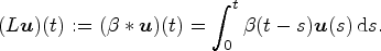
Let us define

\begin{aligned} (L u) (t) := (β * u) (t) = \int_{0}^{t} β (t - s) u (s) d s . \end{aligned}

A function

β (\cdot)

is called positive kernel if the operator L is positive on

L^{2} (0, T; H)

, that is, for all T

\begin{aligned} \int_{0}^{T} (L u (t), u (t)) d t = \int_{0}^{T} \int_{0}^{t} β (t - s) (u (s), u (t)) d s d t ⩾ 0, \end{aligned}

for all u \in H and every T > 0

. Clearly

β (t) = γ e^{- δ t}

is a positive kernel, so that

\begin{aligned} \int_{0}^{T} ⟨ (β * A) u (t), u (t) ⟩ d t = \int_{0}^{T} ((β * \nabla u) (t), \nabla u (t)) d t ⩾ 0. \end{aligned}

(2.4)

2.5. Abstract formulation and weak solution

Taking $P_{H}$ in (1.2), we write the abstract formulation of the system (1.2) as:

\begin{aligned} {\begin{cases} \frac{d u (t)}{d t} + μ A u (t) + (β * A u) (t) + B (u (t), u (t)) = P_{H} f, t \in (0, T), \\ u (0) = u_{0} \in H . \end{cases} \end{aligned}

(2.5)

Let us now provide the definition of weak solution for the system (2.5).

Definition 2.1.

The function $u \in C ([0, T]; H) \cap L^{2} (0, T; V)$ with $\partial_{t} u \in L^{2} (0, T; V^{'})$ , is called a weak solution to the system (2.5), if for $f \in L^{2} (Ω)$ , $u_{0} \in H$ and $ϕ \in V$ , $u (\cdot)$ satisfies for a.e. $t \in [0, T]$

\begin{aligned} {\begin{cases} ⟨ \partial_{t} u (t) + μ A u (t) + (β * A u) (t) + B (u (t)), ϕ ⟩ = (f, ϕ), \\ {lim}_{t ↓ 0} ‖ u (t) - u_{0} ‖_{H} = 0. \end{cases} \end{aligned}

(2.6)

Let us now state the existence and uniqueness theorem for the system (2.5). A proof of the following theorem can be obtained from [34, Theorem 3.4]. A local monotonicity property of the linear and nolinear operators and a generalization of the Minty–Browder technique is exploited in the proof of [34, Theorem 3.4]. Theorem 2.2.

There exists a unique weak solution $u (\cdot)$ to the system (2.5) in the sense of Definition 2.1 satisfying the following energy equality:

\begin{aligned} \frac{1}{2} \frac{d}{d t} ‖ u (t) ‖_{H}^{2} + μ ‖ u (t) ‖_{V}^{2} + (β * \nabla u (t), \nabla u (t)) = (f, u (t)) \end{aligned}

(2.7)

for a.e.

t \in [0, T]

2.6. Kuratowski’s measure of noncompactness

The first result on measure of noncompactness was defined and studied by Kuratowski in [29]. With the help of some vital implications of Kuratowski’s measure of noncompactness, one can show the existence of a convergent subsequence for some arbitrary sequences. Therefore, such results are helpful to obtain the asymptotic compactness of semigroup without using the compact embedding, cf. [24,50,51] etc., and references therein.

Definition 2.3 Kuratowski’s measure of noncompactness, [39]

Let $(X, d)$ be a metric space and E a bounded subset of $X$ . Then the Kuratowski measure of noncompactness (the set-measure of noncompactness) of E, $κ_{X} (E)$ , is defined by

\begin{aligned} κ_{X} (E) = inf {ε > 0 : E \subset ⋃_{i = 1}^{n} Q_{i}, Q_{i} \subset X, diam (Q_{i}) < ε (i = 1, 2 \dots, n; n \in N)} . \end{aligned}

The function κ is called Kuratowski’s measure of noncompactness.

Note that $κ_{X} (E) = 0$ if and only if $\bar{E}$ is compact (see [39, Lemma 1.2]). The following lemma is an application of Kuratowski’s measure of noncompactness which is helpful in proving the asymptotic compactness of the solution operator.

Lemma 2.4 [32, Lemma 2.7]

Let $X$ be a Banach space and ${x_{n}}_{n \in N}$ be an arbitrary sequence in $X$ . Then ${x_{n}}_{n \in N}$ has a convergent subsequence if $κ_{X} ({x_{n} : n ⩾ m}) \to 0 ~as~ m \to \infty$ .

3. Global attractor

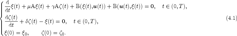
In this section, we discuss the existence of a global attractor for 2D Oldroyd model of fluid flow equations of order one. We assume that $f \in L^{2} (Ω)$ is independent of t in (2.5). Since the system (2.5) depends on memory (non-autonomous), the solution cannot be represented as a one parameter family of semigroups and hence we cannot use the usual theory used in [42] for the autonomous 2D Navier–Stokes equations, to obtain the global attractors. Thus, as we discussed earlier, we use the transformation, $v (t) = \int_{0}^{t} e^{- δ (t - s)} u (s) d s$ and transform the system (2.5) to

\begin{aligned} {\begin{cases} \frac{d u (t)}{d t} + μ A u (t) + γ A v (t) + B (u (t), u (t)) = f, t \in (0, T), \\ \frac{d v (t)}{d t} - u (t) + δ v (t) = 0, t \in (0, T), \\ u (0) = u_{0}, v (0) = 0 . \end{cases} \end{aligned}

(3.1)

Note that whenever a Cauchy problem on a Banach space $X$ is well posed in the sense of Hadamard (for proper notion of weak solution) for all initial data $x (0) = x_{0} \in X$ , then the corresponding (forward) solutions $x (t)$ can be written in the form $x (t) = S (t) x_{0}$ , where the semigroup $S (t)$ is uniquely determined by the dynamical system.

The transformation $v (t) = \int_{0}^{t} e^{- δ (t - s)} u (s) d s$ which converts the original equation (1.2) (or (2.5)) into the autonomous one (1.5) (or (3.1)) does not seem to work. The issue is that all the autonomous attractor theory requires the semigroup $S (t) : X \to X$ , in other words, the allowable space of initial data must be the whole of the phase space. The proof of invariance of the attractor, for example, relies on the fact that $S (t)$ is a semigroup, so that $S (t) S (s) = S (t + s)$ . In this case, the allowable initial data is the space $H \times {0}$ , the evolution under the flow will produce a solution that no longer lies in the space $H \times {0}$ . Therefore, we consider the following system in our further analysis:

\begin{aligned} {\begin{cases} \frac{d u (t)}{d t} + μ A u (t) + γ A v (t) + B (u (t), u (t)) = f, t \in (0, T), \\ \frac{d v (t)}{d t} - u (t) + δ v (t) = 0, t \in (0, T), \\ u (0) = u_{0}, v (0) = v_{0}, \end{cases} \end{aligned}

(3.2)

where

u_{0} \in H

and

v_{0} \in V

. Note that the system (3.1) is a particular case of (3.2).

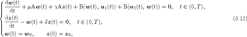
Let us define $U := (u, v)^{⊤}$ , so that $U (\cdot)$ satisfies:

\begin{aligned} {\begin{cases} \frac{dU (t)}{d t} = F - [A U (t) + B (U (t))] = F (U (t)), \\ U (0) = U_{0}, \end{cases} \end{aligned}

(3.3)

where

\begin{aligned} A = (\begin{matrix} μ A & γ A \\ - I & δ I \end{matrix}), B (U) = (\begin{matrix} B (u) \\ 0 \end{matrix}), F = (\begin{matrix} f \\ 0 \end{matrix}) and U_{0} = (\begin{matrix} u_{0} \\ v_{0} \end{matrix}) . \end{aligned}

(3.4)

By a standard Galerkin approximation technique, it can be shown that the system (3.2) has a unique weak solution in

(C ([0, T]; H) \cap L^{2} (0, T; V)) \times C ([0, T]; V)

(see Lemma 3.2 and Proposition 3.4 below). In the sequel, we use the notation,

X = H \times V

with the norm

‖ \cdot ‖_{X} = (‖ \cdot ‖_{H}^{2} + γ ‖ \cdot ‖_{V}^{2})^{1 / 2}

, that is,

‖ U ‖_{X} = ‖ (u, v)^{⊤} ‖_{X} = (‖ u ‖_{H}^{2} + γ ‖ v ‖_{V}^{2})^{1 / 2}

. It can be easily seen that

\begin{aligned} min {1, γ} (‖ u ‖_{H}^{2} + ‖ v ‖_{V}^{2}) ⩽ ‖ u ‖_{H}^{2} + γ ‖ v ‖_{V}^{2} ⩽ max {1, γ} (‖ u ‖_{H}^{2} + ‖ v ‖_{V}^{2}), \end{aligned}

and hence the norms

{‖ u ‖_{H}^{2} + ‖ v ‖_{V}^{2}}^{1 / 2}

and

{‖ u ‖_{H}^{2} + γ ‖ v ‖_{V}^{2}}^{1 / 2}

are equivalent on

X

Let $U (t)$ , $t ⩾ 0$ be the unique weak solution of the system (3.2). Thanks to the existence and uniqueness of weak solution for the system (3.3), we can define a continuous semigroup ${S (t)}_{t ⩾ 0}$ in $X$ by

\begin{aligned} S (t) U_{0} = U (t), t ⩾ 0, \end{aligned}

(3.5)

where

U (\cdot)

is the unique weak solution of (3.3) with

U (0) = U_{0} \in X

It should be noted that the system (3.2) is autonomous and hence we can develop a similar theory available in [42] for the system (3.2). We prove the existence of a global attractor for the system (3.2) in Poincaré domains satisfying Hypothesis 1.1. This follows from the following general result:

Theorem 3.1 [48, Theorem I.1.1], [31,42]

Let $E$ be a complete metric space and let ${S (t)}_{t ⩾ 0}$ be a semigroup of continuous (nonlinear) operators in $E$ . If (and only if) ${S (t)}_{t ⩾ 0}$ possesses an absorbing set $B$ bounded in $E$ and is asymptotically compact in $E$ , then ${S (t)}_{t ⩾ 0}$ possesses a (compact) global attractor $A = ω (B)$ . Furthermore, if $t \mapsto S (t) U_{0}$ is continuous from $R^{+}$ into $E$ and $B$ is connected in $E$ , then $A$ is connected in $E$ .

Let us next prove the existence of a global attractor for the semigroup $S (t), t ⩾ 0$ defined on $X$ for the 2D Oldroyd system (3.2) in Poincaré domains. Our first aim is to establish the existence of an absorbing ball in $X$ for $S (t), t ⩾ 0$ . Next lemma provides an estimate satisfied by $U (\cdot)$ which will be useful in the sequel.

Lemma 3.2.
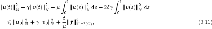
Let $U (\cdot) = (u (\cdot), v (\cdot))^{⊤}$ be the unique weak solution of the system ( 3.2 ). Then, we have for all $t > 0$
$\begin{aligned} \frac{1}{t} \int_{0}^{t} [‖ u (s) ‖_{V}^{2} + γ ‖ v (s) ‖_{V}^{2}] d s ⩽ \frac{1}{min {μ, 2 δ}} {\frac{‖ u_{0} ‖_{H}^{2} + γ ‖ v_{0} ‖_{V}^{2}}{t} + \frac{1}{μ} ‖ f ‖_{H^{- 1} (Ω)}^{2}} . \end{aligned}$
(3.6)

Proof.
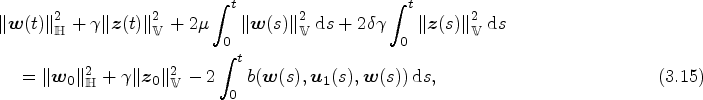
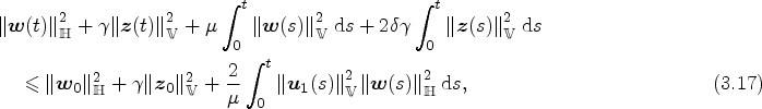
Let us take the inner product with $u (\cdot)$ to the first equation in (3.2) to get
$\begin{aligned} \frac{1}{2} \frac{d}{d t} ‖ u (t) ‖_{H}^{2} + μ ‖ \nabla u (t) ‖_{H}^{2} = - γ (\nabla v (t), \nabla u (t)) + ⟨ f, u (t) ⟩, \end{aligned}$
(3.7)
for a.e. $t \in [0, T]$ , where we have used $⟨ B (u), u ⟩ = 0$ . Taking the inner product with $γ A v (\cdot)$ to the second equation in (2.5), we obtain
$\begin{aligned} \frac{1}{2} \frac{d}{d t} (γ ‖ v (t) ‖_{V}^{2}) + δ γ ‖ v (t) ‖_{V}^{2} = γ (\nabla u (t), \nabla v (t)), \end{aligned}$
(3.8)
for a.e. $t \in [0, T]$ . Adding (3.7) and (3.8), we arrive at
$\begin{aligned} \frac{1}{2} \frac{d}{d t} [‖ u (t) ‖_{H}^{2} + γ ‖ v (t) ‖_{V}^{2}] + μ ‖ u (t) ‖_{V}^{2} + γ δ ‖ v (t) ‖_{V}^{2} = ⟨ f, u (t) ⟩, \end{aligned}$
(3.9)
for a.e. $t \in [0, T]$ . Using the Cauchy–Schwarz and Young’s inequalities, we estimate $⟨ f, u ⟩$ as
$\begin{aligned} | ⟨ f, u ⟩ | ⩽ ‖ f ‖_{H^{- 1} (Ω)} ‖ u ‖_{V} ⩽ \frac{μ}{2} ‖ u ‖_{V}^{2} + \frac{1}{2 μ} ‖ f ‖_{H^{- 1} (Ω)}^{2} . \end{aligned}$
(3.10)
Applying (3.10) in (3.7) and then integrating from 0 to t, we obtain
$\begin{aligned} {‖ u (t) ‖}_{H}^{2} + γ {‖ v (t) ‖}_{V}^{2} + μ \int_{0}^{t} {‖ u (s) ‖}_{V}^{2} d s + 2 δ γ \int_{0}^{t} {‖ v (s) ‖}_{V}^{2} d s \\ ⩽ ‖ u_{0} ‖_{H}^{2} + γ ‖ v_{0} ‖_{V}^{2} + \frac{t}{μ} ‖ f ‖_{H^{- 1} (Ω)}^{2}, \end{aligned}$
(3.11)
for $t > 0$ . From (3.11), one can easily derive (3.6).

In the next lemma, we show that the operator $S (t) : X \to X$ , for $t ⩾ 0$ , is Lipschitz continuous on bounded subsets of $X$ . Lemma 3.3.
The map $S (t) : X \to X$ , for $t ⩾ 0$ , is Lipschitz continuous on bounded subsets of $X$ .
Proof.
Let us take $S (t) U_{0} = U (t) = (u_{1} (t), v_{1} (t))^{⊤}$ and $S (t) V_{0} = V (t) = (u_{2} (t), v_{2} (t))^{⊤}$ , for all $t ⩾ 0$ . Then $W (t) := U (t) - V (t) = (w (t), z (t))^{⊤}$ satisfies:
$\begin{aligned} {\begin{cases} \frac{d w (t)}{d t} + μ A w (t) + γ A z (t) + B (w (t), u_{1} (t)) + B (u_{2} (t), w (t)) = 0, t \in (0, T), \\ \frac{d z (t)}{d t} - w (t) + δ z (t) = 0, t \in (0, T), \\ w (0) = w_{0}, z (0) = z_{0}, \end{cases} \end{aligned}$
(3.12)
where, $w_{0} \in H$ and $z_{0} \in V$ . Let us take the inner product with $w (t)$ in the first equation in (3.12) to find
$\begin{aligned} \frac{1}{2} \frac{d}{d t} ‖ w (t) ‖_{H}^{2} + μ ‖ \nabla w (t) ‖_{H}^{2} = - γ (\nabla z (t), \nabla w (t)) - b (w (t), u_{1} (t), w (t)), \end{aligned}$
(3.13)
for a.e. $t \in [0, T]$ , where we have used the fact that $b (u_{2}, w, w) = 0$ . Next, we take the inner product with $γ A z (\cdot)$ to the second equation in (3.12) to get
$\begin{aligned} \frac{1}{2} \frac{d}{d t} (γ ‖ z (t) ‖_{V}^{2}) + δ γ ‖ z (t) ‖_{V}^{2} = γ (\nabla w (t), \nabla z (t)), \end{aligned}$
(3.14)
for a.e. $t \in [0, T]$ . Adding (3.13) and (3.14), and integrating from 0 to t, we obtain
$\begin{aligned} {‖ w (t) ‖}_{H}^{2} + γ {‖ z (t) ‖}_{V}^{2} + 2 μ \int_{0}^{t} {‖ w (s) ‖}_{V}^{2} d s + 2 δ γ \int_{0}^{t} {‖ z (s) ‖}_{V}^{2} d s \\ = ‖ w_{0} ‖_{H}^{2} + γ ‖ z_{0} ‖_{V}^{2} - 2 \int_{0}^{t} b (w (s), u_{1} (s), w (s)) d s, \end{aligned}$
(3.15)
for all $t \in [0, T]$ . Using Hölder’s and Ladyzhenskaya’s inequalities, we estimate $| b (w, u_{1}, w) |$ as
$\begin{aligned} | b (w, u_{1}, w) | ⩽ ‖ w ‖_{L^{4}}^{2} ‖ \nabla u_{1} ‖_{H} ⩽ \sqrt{2} ‖ w ‖_{H} ‖ \nabla w ‖_{H} ‖ \nabla u_{1} ‖_{H} ⩽ \frac{μ}{2} ‖ w ‖_{V}^{2} + \frac{1}{μ} ‖ u_{1} ‖_{V}^{2} ‖ w ‖_{H}^{2} . \end{aligned}$
(3.16)
Let us use (3.16) in (3.15) to deduce
$\begin{aligned} {‖ w (t) ‖}_{H}^{2} + γ {‖ z (t) ‖}_{V}^{2} + μ \int_{0}^{t} {‖ w (s) ‖}_{V}^{2} d s + 2 δ γ \int_{0}^{t} {‖ z (s) ‖}_{V}^{2} d s \\ ⩽ ‖ w_{0} ‖_{H}^{2} + γ ‖ z_{0} ‖_{V}^{2} + \frac{2}{μ} \int_{0}^{t} {‖ u_{1} (s) ‖}_{V}^{2} {‖ w (s) ‖}_{H}^{2} d s, \end{aligned}$
(3.17)
for all $t \in [0, T]$ . Applying Gronwall’s inequality in (3.17), we obtain
$\begin{aligned} ‖ w (t) ‖_{H}^{2} + γ ‖ z (t) ‖_{V}^{2} ⩽ [‖ w_{0} ‖_{H}^{2} + γ ‖ z_{0} ‖_{V}^{2}] \exp (\frac{2}{μ} \int_{0}^{t} ‖ u_{1} (s) ‖_{V}^{2} d s), \end{aligned}$
(3.18)
for all $t \in [0, T]$ . Thus, it is immediate that
$\begin{aligned} ‖ S (t) U_{0} - S (t) V_{0} ‖_{X} & ⩽ ‖ U_{0} - V_{0} ‖_{X} \exp (\frac{1}{μ} \int_{0}^{t} {‖ u_{1} (s) ‖}_{V}^{2} d s) \\ ⩽ ‖ U_{0} - V_{0} ‖_{X} \exp {\frac{1}{μ^{2}} (‖ U_{0} ‖_{X}^{2} + \frac{t}{μ} ‖ f ‖_{H^{- 1} (Ω)}^{2})}, \end{aligned}$
(3.19)
for all $t \in [0, T]$ , where we have used (3.11). Thus, the map $S (t) : X \to X$ , for $t ⩾ 0$ , is Lipschitz continuous on bounded subsets of $X$ .

3.1. Absorbing ball in $X$

In this subsection, we show that the semigroup $S (t)$ has an absorbing set in $X$ .

Proposition 3.4.
The set
$\begin{aligned} B_{1} := {V \in X : ‖ V ‖_{X} ⩽ M_{1} \equiv \sqrt{\frac{2}{μ α}} ‖ f ‖_{H^{- 1} (Ω)}}, \end{aligned}$
(3.20)
where $α = min {\frac{3 μ λ}{4}, 2 δ}$ , is an absorbing set in $X$ for the semigroup $S (t)$ . That is, given a bounded set $B \subset X$ , there exists an entering time $t_{B} > 0$ such that $S (t) B \subset B_{1}$ , for all $t ⩾ t_{B}$ .
Proof.
Let $(u_{0}, v_{0})^{⊤} \in B$ . From (3.9), we have
$\begin{aligned} \frac{d}{d t} [‖ u (t) ‖_{H}^{2} + γ ‖ v (t) ‖_{V}^{2}] + \frac{3 μ λ}{4} ‖ u (t) ‖_{H}^{2} + 2 γ δ ‖ v (t) ‖_{V}^{2} + \frac{μ}{4} ‖ u (t) ‖_{V}^{2} ⩽ \frac{1}{μ} ‖ f ‖_{H^{- 1} (Ω)}^{2}, \end{aligned}$
(3.21)
for a.e. $t \in [0, T]$ , and an application of Gronwall’s inequality yields
$\begin{aligned} {‖ u (t) ‖}_{H}^{2} + γ {‖ v (t) ‖}_{V}^{2} + \frac{μ}{4} \int_{0}^{t} e^{- α (t - s)} {‖ u (s) ‖}_{V}^{2} d s \\ ⩽ [‖ u_{0} ‖_{H}^{2} + γ ‖ v_{0} ‖_{V}^{2}] e^{- α t} + \frac{1}{μ α} ‖ f ‖_{H^{- 1} (Ω)}^{2}, \end{aligned}$
(3.22)
for all $t ⩾ 0$ , where $α = min {\frac{3 μ λ}{4}, 2 δ}$ . Moreover, we observe
$\begin{aligned} \underset{t \to \infty}{\lim \sup} [‖ u (t) ‖_{H}^{2} + γ ‖ v (t) ‖_{V}^{2} + \frac{μ}{4} \int_{0}^{t} e^{- α (t - s)} ‖ u (s) ‖_{V}^{2} d s] ⩽ \frac{1}{μ α} ‖ f ‖_{H^{- 1} (Ω)}^{2}, \end{aligned}$
(3.23)
which implies that there exists a time $t_{B} ⩾ 0$ such that
$\begin{aligned} [‖ u (t) ‖_{H}^{2} + γ ‖ v (t) ‖_{V}^{2} + \frac{μ}{4} \int_{0}^{t} e^{- α (t - s)} ‖ u (s) ‖_{V}^{2} d s] ⩽ \frac{2}{μ α} ‖ f ‖_{H^{- 1} (Ω)}^{2}, \end{aligned}$
(3.24)
for all $t ⩾ t_{B}$ . Also, we obtain from (3.23) that
$\begin{aligned} \underset{t \to \infty}{\lim \sup} ‖ U (t) ‖_{X} ⩽ \frac{1}{\sqrt{μ α}} ‖ f ‖_{H^{- 1} (Ω)} . \end{aligned}$
(3.25)
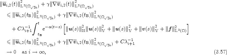
Furthermore, it follows from (3.22) and (3.25) that the set (3.20) is absorbing in $X$ for the semigroup $S (t)$ . Hence, the following uniform estimate is valid:
$\begin{aligned} ‖ U (t) ‖_{X} ⩽ M_{1}, where M_{1} = \sqrt{\frac{2}{μ α}} ‖ f ‖_{H^{- 1} (Ω)}, \end{aligned}$
(3.26)
for t large enough ( $t ≫ 1$ or $t ⩾ t_{B}$ ) depending on the initial data.

3.2. Asymptotic compactness

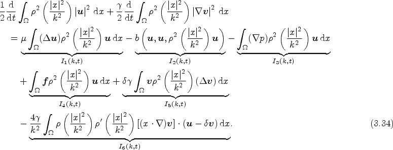
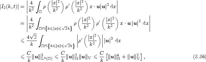
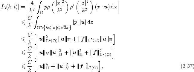
In this subsection, we establish the asymptotic compactness of the semigroup ${S (t)}_{t ⩾ 0}$ associated with the system (3.2). We show the asymptotic compactness with the help of uniform-tail estimate, flattening property and an application of Kuratowski’s measure of noncompactness (see Lemma 2.4). In the following lemma, we obtain the uniform-tail estimates for the solutions of the system (3.2).

Let ρ be a smooth function such that $0 ⩽ ρ (ξ) ⩽ 1$ for $ξ \in R$ and

\begin{aligned} ρ (ξ) = {\begin{cases} 0, & for | ξ | ⩽ 1, \\ 1, & for | ξ | ⩾ 2. \end{cases} \end{aligned}

(3.27)

Then, there exists a positive constant C such that

| ρ^{'} (ξ) | ⩽ C

and

| ρ^{″} (ξ) | ⩽ C

for all

ξ \in R

Lemma 3.5.

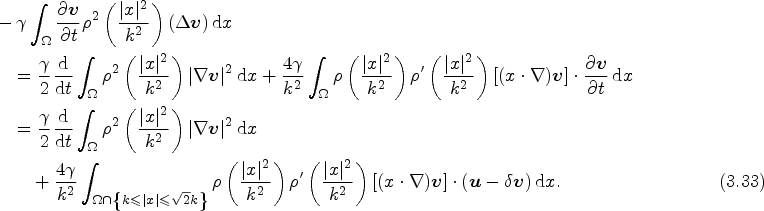
Suppose that $f \in L^{2} (Ω)$ . Then for every $ε > 0$ , there exists $k_{0} \in N$ such that the solution $U (\cdot)$ of system ( 1.5 ) satisfies

\begin{aligned} {| | ρ (\frac{| \cdot |^{2}}{k^{2}}) U (t) | |}_{L^{2} {(Ω}_{k}^{c}) \times H_{0}^{1} {(Ω}_{k}^{c})} ⩽ ε, \end{aligned}

(3.28)

for all

t ⩾ t_{B}

and for all

k ⩾ k_{0}

, where

Ω_{k}^{c} = Ω ∖ Ω_{k}

and

Ω_{k} = {x \in Ω : | x | ⩽ k}

Proof.

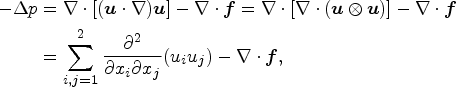
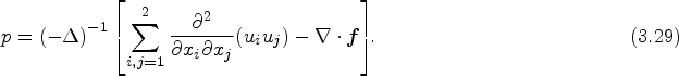
Taking the divergence of the first equation of (1.5), we obtain

\begin{aligned} - Δ p & = \nabla \cdot [(u \cdot \nabla) u] - \nabla \cdot f = \nabla \cdot [\nabla \cdot (u \otimes u)] - \nabla \cdot f \\ = \sum_{i, j = 1}^{2} \frac{\partial^{2}}{\partial x_{i} \partial x_{j}} (u_{i} u_{j}) - \nabla \cdot f, \end{aligned}

in the weak sense which implies that

\begin{aligned} p = {(- Δ)}^{- 1} [\sum_{i, j = 1}^{2} \frac{\partial^{2}}{\partial x_{i} \partial x_{j}} (u_{i} u_{j}) - \nabla \cdot f] . \end{aligned}

(3.29)

It follows from (3.29) that

\begin{aligned} ‖ p ‖_{L^{2} (Ω)} & ⩽ {‖ [\sum_{i, j = 1}^{2} \frac{\partial^{2}}{\partial x_{i} \partial x_{j}} (- Δ)^{- 1} (u_{i} u_{j})] ‖}_{L^{2} (Ω)} + ‖ (- Δ)^{- 1} (\nabla \cdot f) ‖_{L^{2} (Ω)} \\ ⩽ C {‖ \sum_{i, j = 1}^{2} (- Δ)^{- 1} (u_{i} u_{j}) ‖}_{H^{2} (Ω)} + C ‖ \nabla \cdot f ‖_{H^{- 2} (Ω)} \\ ⩽ C {‖ Δ \sum_{i, j = 1}^{2} (- Δ)^{- 1} (u_{i} u_{j}) ‖}_{L^{2} (Ω)} + C ‖ f ‖_{H^{- 1} (Ω)} \\ ⩽ C ‖ u ‖_{L^{4} (Ω)}^{2} + C ‖ f ‖_{L^{2} (Ω)}, \end{aligned}

(3.30)

where, in the second and third steps, we have used the elliptic regularity for Poincaré domains with uniformly smooth boundary of class

C^{3}

(cf. [18, Lemma 1]). Taking the inner product of the first equation of (1.5) with

ρ^{2} (\frac{| x |^{2}}{k^{2}}) u

and the second equation of (1.5) with

- γ ρ^{2} (\frac{| x |^{2}}{k^{2}}) (Δ v)

L^{2} (Ω)

, we have

\begin{aligned} \frac{1}{2} \frac{d}{d t} \int_{Ω} ρ^{2} (\frac{| x |^{2}}{k^{2}}) | u |^{2} d x \\ = μ \int_{Ω} (Δ u) ρ^{2} (\frac{| x |^{2}}{k^{2}}) u d x - b (u, u, ρ^{2} (\frac{| x |^{2}}{k^{2}}) u) + γ \int_{Ω} (Δ v) ρ^{2} (\frac{| x |^{2}}{k^{2}}) u d x \\ - \int_{Ω} (\nabla p) ρ^{2} (\frac{| x |^{2}}{k^{2}}) u d x + \int_{Ω} f ρ^{2} (\frac{| x |^{2}}{k^{2}}) u d x, \end{aligned}

(3.31)

and

\begin{aligned} - γ \int_{Ω} \frac{\partial v}{\partial t} ρ^{2} (\frac{| x |^{2}}{k^{2}}) (Δ v) d x = - γ \int_{Ω} u ρ^{2} (\frac{| x |^{2}}{k^{2}}) (Δ v) d x + δ γ \int_{Ω} v ρ^{2} (\frac{| x |^{2}}{k^{2}}) (Δ v) d x . \end{aligned}

(3.32)

An integration by parts gives

\begin{aligned} - γ \int_{Ω} \frac{\partial v}{\partial t} ρ^{2} (\frac{| x |^{2}}{k^{2}}) (Δ v) d x \\ = \frac{γ}{2} \frac{d}{d t} \int_{Ω} ρ^{2} (\frac{| x |^{2}}{k^{2}}) | \nabla v |^{2} d x + \frac{4 γ}{k^{2}} \int_{Ω} ρ (\frac{| x |^{2}}{k^{2}}) ρ^{'} (\frac{| x |^{2}}{k^{2}}) [(x \cdot \nabla) v] \cdot \frac{\partial v}{\partial t} d x \\ = \frac{γ}{2} \frac{d}{d t} \int_{Ω} ρ^{2} (\frac{| x |^{2}}{k^{2}}) | \nabla v |^{2} d x \\ + \frac{4 γ}{k^{2}} \int_{Ω \cap {k ⩽ | x | ⩽ \sqrt{2} k}} ρ (\frac{| x |^{2}}{k^{2}}) ρ^{'} (\frac{| x |^{2}}{k^{2}}) [(x \cdot \nabla) v] \cdot (u - δ v) d x . \end{aligned}

(3.33)

Adding (3.31)–(3.33), we obtain

\begin{aligned} \frac{1}{2} \frac{d}{d t} \int_{Ω} ρ^{2} (\frac{| x |^{2}}{k^{2}}) {| u |}^{2} d x + \frac{γ}{2} \frac{d}{d t} \int_{Ω} ρ^{2} (\frac{| x |^{2}}{k^{2}}) {| \nabla v |}^{2} d x \\ = \underset{I_{1} (k, t)}{\underset{⏟}{μ \int_{Ω} (Δ u) ρ^{2} (\frac{| x |^{2}}{k^{2}}) u d x}} - \underset{I_{2} (k, t)}{\underset{⏟}{b (u, u, ρ^{2} (\frac{| x |^{2}}{k^{2}}) u)}} - \underset{I_{3} (k, t)}{\underset{⏟}{\int_{Ω} (\nabla p) ρ^{2} (\frac{| x |^{2}}{k^{2}}) u d x}} \\ + \underset{I_{4} (k, t)}{\underset{⏟}{\int_{Ω} f ρ^{2} (\frac{| x |^{2}}{k^{2}}) u d x}} + \underset{I_{5} (k, t)}{\underset{⏟}{δ γ \int_{Ω} v ρ^{2} (\frac{| x |^{2}}{k^{2}}) (Δ v) d x}} \\ - \underset{I_{6} (k, t)}{\underset{⏟}{\frac{4 γ}{k^{2}} \int_{Ω} ρ (\frac{| x |^{2}}{k^{2}}) ρ^{'} (\frac{| x |^{2}}{k^{2}}) [(x \cdot \nabla) v] \cdot (u - δ v) d x}} . \end{aligned}

(3.34)

Let us now estimate each term on the right hand side of (3.34). By (1.1), integration by parts, the fact that $u$ is divergence free, and (3.30), we have

\begin{aligned} I_{1} (k, t) & = - μ \int_{Ω} {| \nabla (ρ (\frac{| x |^{2}}{k^{2}}) u) |}^{2} d x + μ \int_{Ω} u \nabla (ρ (\frac{| x |^{2}}{k^{2}})) \nabla (ρ (\frac{| x |^{2}}{k^{2}}) u) d x \\ - μ \int_{Ω} \nabla u \nabla (ρ (\frac{| x |^{2}}{k^{2}})) ρ (\frac{| x |^{2}}{k^{2}}) u d x \\ ⩽ - μ \int_{Ω} {| \nabla (ρ (\frac{| x |^{2}}{k^{2}}) u) |}^{2} d x + \frac{μ}{8} \int_{Ω} {| \nabla (ρ (\frac{| x |^{2}}{k^{2}}) u) |}^{2} d x \\ + \frac{μ λ}{8} \int_{Ω} ρ^{2} (\frac{| x |^{2}}{k^{2}}) {| u |}^{2} d x + \frac{C}{k} [‖ u ‖_{H}^{2} + ‖ u ‖_{V}^{2}] \\ ⩽ - \frac{3 μ λ}{4} \int_{Ω} ρ^{2} (\frac{| x |^{2}}{k^{2}}) {| u |}^{2} d x + \frac{C}{k} ‖ u ‖_{V}^{2}, \end{aligned}

(3.35)

\begin{aligned} | I_{2} (k, t) | & = | \frac{4}{k^{2}} \int_{Ω} ρ (\frac{| x |^{2}}{k^{2}}) ρ^{'} (\frac{| x |^{2}}{k^{2}}) x \cdot u | u |^{2} d x | \\ = | \frac{4}{k^{2}} \int_{Ω \cap {k ⩽ | x | ⩽ \sqrt{2} k}} ρ (\frac{| x |^{2}}{k^{2}}) ρ^{'} (\frac{| x |^{2}}{k^{2}}) x \cdot u {| u |}^{2} d x | \\ ⩽ \frac{4 \sqrt{2}}{k} \int_{Ω \cap {k ⩽ | x | ⩽ \sqrt{2} k}} | ρ^{'} (\frac{| x |^{2}}{k^{2}}) | {| u |}^{3} d x \\ ⩽ \frac{C}{k} ‖ u ‖_{L^{3} (Ω)}^{3} ⩽ \frac{C}{k} ‖ u ‖_{H}^{2} ‖ u ‖_{V} ⩽ \frac{C}{k} [‖ u ‖_{H}^{4} + ‖ u ‖_{V}^{2}], \end{aligned}

(3.36)

\begin{aligned} | I_{3} (k, t) | & = | \frac{4}{k^{2}} \int_{Ω} p ρ (\frac{| x |^{2}}{k^{2}}) ρ^{'} (\frac{| x |^{2}}{k^{2}}) (x \cdot u) d x | \\ ⩽ \frac{C}{k} \int_{Ω \cap {k ⩽ | x | ⩽ \sqrt{2} k}} | p | | u | d x \\ ⩽ \frac{C}{k} [‖ u ‖_{L^{4} (Ω)}^{2} ‖ u ‖_{H} + ‖ f ‖_{L^{2} (Ω)} ‖ u ‖_{H}] \\ ⩽ \frac{C}{k} [‖ u ‖_{V} ‖ u ‖_{H}^{2} + ‖ u ‖_{H}^{2} + ‖ f ‖_{L^{2} (Ω)}^{2}] \\ ⩽ \frac{C}{k} [‖ u ‖_{H}^{4} + ‖ u ‖_{V}^{2} + ‖ f ‖_{L^{2} (Ω)}^{2}], \end{aligned}

(3.37)

where we have used Gagliardo–Nirenberg’s and Young’s inequalities also. A similar argument as in (3.35) yields

\begin{aligned} I_{5} (k, t) & = - δ γ \int_{Ω} ρ^{2} (\frac{| x |^{2}}{k^{2}}) {| \nabla v |}^{2} d x - \frac{4 δ γ}{k^{2}} \int_{Ω} ρ (\frac{| x |^{2}}{k^{2}}) ρ^{'} (\frac{| x |^{2}}{k^{2}}) [(x \cdot \nabla) v] \cdot v d x \\ ⩽ - δ γ \int_{Ω} ρ^{2} (\frac{| x |^{2}}{k^{2}}) {| \nabla v |}^{2} d x + \frac{C}{k} ‖ v ‖_{H}^{2} . \end{aligned}

(3.38)

In view of the Cauchy–Schwarz and Young’s inequalities, we estimate

\begin{aligned} | I_{4} (k, t) | & ⩽ \frac{3 μ λ}{8} \int_{Ω} ρ^{2} (\frac{| x |^{2}}{k^{2}}) | u |^{2} d x + C \int_{Ω} ρ^{2} (\frac{| x |^{2}}{k^{2}}) | f |^{2} d x, \end{aligned}

(3.39)

\begin{aligned} | I_{6} (k, t) | & ⩽ \frac{C}{k} [‖ u ‖_{H}^{2} + ‖ v ‖_{V}^{2}] ⩽ \frac{C}{k} [‖ u ‖_{V}^{2} + ‖ v ‖_{V}^{2}] . \end{aligned}

(3.40)

Now, combining (3.34)–(3.40), we find for

α = min {\frac{3 μ λ}{4}, 2 δ}

\begin{aligned} \frac{d}{d t} [\frac{1}{2} \int_{Ω} ρ^{2} (\frac{| x |^{2}}{k^{2}}) {| u |}^{2} d x + \frac{γ}{2} \int_{Ω} ρ^{2} (\frac{| x |^{2}}{k^{2}}) {| \nabla v |}^{2} d x] \\ + α [\frac{1}{2} \int_{Ω} ρ^{2} (\frac{| x |^{2}}{k^{2}}) {| u |}^{2} d x + \frac{γ}{2} \int_{Ω} ρ^{2} (\frac{| x |^{2}}{k^{2}}) {| \nabla v |}^{2} d x] \\ ⩽ \frac{C}{k} [‖ u ‖_{H}^{4} + ‖ u ‖_{V}^{2} + ‖ v ‖_{V}^{2} + ‖ f ‖_{L^{2} (Ω)}^{2}] + C \int_{Ω} ρ^{2} (\frac{| x |^{2}}{k^{2}}) {| f |}^{2} d x . \end{aligned}

(3.41)

For

t ⩾ t_{B}

, an application of variation of constants formula yields

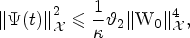
\begin{aligned} \frac{1}{2} \int_{Ω} ρ^{2} (\frac{| x |^{2}}{k^{2}}) {| u (x, t) |}^{2} d x + \frac{γ}{2} \int_{Ω} ρ^{2} (\frac{| x |^{2}}{k^{2}}) {| \nabla v (x, t) |}^{2} d x \\ ⩽ [\frac{1}{2} \int_{Ω} ρ^{2} (\frac{| x |^{2}}{k^{2}}) {| u (x, t_{B}) |}^{2} d x + \frac{γ}{2} \int_{Ω} ρ^{2} (\frac{| x |^{2}}{k^{2}}) {| \nabla v (x, t_{B}) |}^{2} d x] e^{- α t} \\ + \frac{C}{k} \int_{t_{B}}^{t} e^{- α (t - s)} [{‖ u (s) ‖}_{H}^{4} + {‖ u (s) ‖}_{V}^{2} + {‖ v (s) ‖}_{V}^{2} + ‖ f ‖_{L^{2} (Ω)}^{2}] d s \\ + C \int_{t_{B}}^{t} e^{- α (t - s)} \int_{Ω} ρ^{2} (\frac{| x |^{2}}{k^{2}}) {| f (x) |}^{2} d x d s \\ ⩽ \int_{Ω \cap {| x | ⩾ k}} {| u (x, t_{B}) |}^{2} d x + \frac{γ}{2} \int_{Ω \cap {| x | ⩾ k}} {| \nabla v (x, t_{B}) |}^{2} d x + \frac{C}{k} + C \int_{Ω \cap {| x | ⩾ k}} {| f (x) |}^{2} d x \\ \to 0 as k \to \infty, \end{aligned}

(3.42)

where we have used the bound obtained in (3.24). Hence, from (3.42), we conclude that for any

ε > 0

, there exists a

k_{0} \in N

such that

\begin{aligned} \int_{Ω \cap {| x | ⩾ k}} ρ^{2} (\frac{| x |^{2}}{k^{2}}) [{| u (x, t) |}^{2} + γ {| \nabla v (x, t) |}^{2}] d x ⩽ ε, \end{aligned}

(3.43)

for all

k ⩾ k_{0}

and

t ⩾ t_{B}

. This completes the proof.

The following lemma provides the flattening estimates for the solution of the system (3.2). For each $k ⩾ 1$ , we set

\begin{aligned} ϱ_{k} (x) := 1 - ρ (\frac{| x |^{2}}{k^{2}}), x \in Ω . \end{aligned}

(3.44)

Let

\bar{u} := ϱ_{k} u

for

u \in H

. Then

\bar{u} \in L^{2} (Ω_{\sqrt{2} k})

, which has the orthogonal decomposition:

\begin{aligned} \bar{u} = P_{i} \bar{u} \oplus (I - P_{i}) \bar{u} =: {\bar{u}}_{i, 1} + {\bar{u}}_{i, 2}, for each i \in N, \end{aligned}

(3.45)

where

P_{i} : L^{2} (Ω_{\sqrt{2} k}) \to H_{i} := span {e_{1}, e_{2}, \dots, e_{i}} \subset L^{2} (Ω_{\sqrt{2} k})

is a canonical projection and

{e_{m}}_{m = 1}^{\infty}

is a family of eigenfunctions of the Dirichlet Laplacian

- Δ

L^{2} (Ω_{\sqrt{2} k})

with the corresponding eigenvalues

0 < λ_{1} ⩽ λ_{2} ⩽ \dots ⩽ λ_{m} \to \infty

m \to \infty

. We also have that

\begin{aligned} ϱ_{k} Δ u = Δ \bar{u} - u Δ ϱ_{k} - 2 \nabla ϱ_{k} \cdot \nabla u . \end{aligned}

Furthermore, for

ψ \in H_{0}^{1} (Ω_{\sqrt{2} k})

, we have

\begin{aligned} P_{i} ψ = \sum_{m = 1}^{i} (ψ, e_{m}) e_{m}, (- Δ)^{1 / 2} P_{i} ψ = \sum_{m = 1}^{i} λ_{j}^{1 / 2} (ψ, e_{m}) e_{m}, \\ (I - P_{i}) ψ = \sum_{m = i + 1}^{\infty} (ψ, e_{m}) e_{m}, (- Δ)^{1 / 2} (I - P_{i}) ψ = \sum_{m = i + 1}^{\infty} λ_{m}^{1 / 2} (ψ, e_{m}) e_{m}, \\ ‖ \nabla (I - P_{i}) ψ ‖_{L^{2} (Ω_{\sqrt{2} k})}^{2} = ‖ (- {Δ)}^{1 / 2} (I - P_{i}) ψ ‖_{L^{2} (Ω_{\sqrt{2} k})}^{2} = \sum_{m = i + 1}^{\infty} λ_{m} {| (ψ, e_{m}) |}^{2} \\ ⩾ λ_{i + 1} \sum_{m = i + 1}^{\infty} {| (ψ, e_{m}) |}^{2} = λ_{i + 1} ‖ (I - P_{i}) ψ ‖_{L^{2} (Ω_{\sqrt{2} k})}^{2} . \end{aligned}

(3.46)

Lemma 3.6.

Suppose that $f \in L^{2} (Ω)$ . Then for every $ε > 0$ and for each $k \in N$ , there exists $i_{0} \in N$ such that the solution $U (\cdot)$ of the system ( 1.5 ) satisfies

\begin{aligned} {| | (I - P_{i}) ϱ_{k} U (t) | |}_{L^{2} (Ω_{\sqrt{2} k}) \times H_{0}^{1} (Ω_{\sqrt{2} k})} ⩽ ε, \end{aligned}

(3.47)

for all

t ⩾ t_{B}

and for all

i ⩾ i_{0}

Proof.

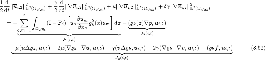
Multiplying the first and second equations of (1.5) by $ϱ_{k}$ , we find

\begin{aligned} \frac{d \bar{u}}{d t} - μ Δ \bar{u} - γ Δ \bar{v} + ϱ_{k} (u \cdot \nabla) u + ϱ_{k} \nabla p \\ = - μ u Δ ϱ_{k} - 2 μ \nabla ϱ_{k} \cdot \nabla u - γ v Δ ϱ_{k} - 2 γ \nabla ϱ_{k} \cdot \nabla v + ϱ_{k} f, \end{aligned}

(3.48)

and

\begin{aligned} \frac{d \bar{v}}{d t} - \bar{u} + δ \bar{v} = 0. \end{aligned}

(3.49)

Applying

(I - P_{i})

to the equations (3.48)–(3.49) and then taking the inner product of the resulting equations with

{\bar{u}}_{i, 2}

and

- γ Δ {\bar{v}}_{i, 2}

L^{2} (Ω_{\sqrt{2} k})

, respectively, we get

\begin{aligned} \frac{1}{2} \frac{d}{d t} ‖ {\bar{u}}_{i, 2} ‖_{L^{2} (Ω_{\sqrt{2} k})}^{2} + μ ‖ \nabla {\bar{u}}_{i, 2} ‖_{L^{2} (Ω_{\sqrt{2} k})}^{2} \\ = γ (Δ {\bar{v}}_{i, 2}, {\bar{u}}_{i, 2}) - \sum_{q, m = 1}^{2} \int_{Ω_{\sqrt{2} k}} (I - P_{i}) [u_{q} \frac{\partial u_{m}}{\partial x_{q}} ϱ_{k}^{2} (x) u_{m}] d x - μ (u Δ ϱ_{k}, {\bar{u}}_{i, 2}) \\ - 2 μ (\nabla ϱ_{k} \cdot \nabla u, {\bar{u}}_{i, 2}) - γ (v Δ ϱ_{k}, {\bar{u}}_{i, 2}) - 2 γ (\nabla ϱ_{k} \cdot \nabla v, {\bar{u}}_{i, 2}) + (ϱ_{k} f, {\bar{u}}_{i, 2}) \\ - (ϱ_{k} (x) \nabla p, {\bar{u}}_{i, 2}), \end{aligned}

(3.50)

and

\begin{aligned} \frac{γ}{2} \frac{d}{d t} ‖ \nabla {\bar{v}}_{i, 2} ‖_{L^{2} (Ω_{\sqrt{2} k})}^{2} + γ ({\bar{u}}_{i, 2}, Δ {\bar{v}}_{i, 2}) + δ γ ‖ \nabla {\bar{v}}_{i, 2} ‖_{L^{2} (Ω_{\sqrt{2} k})}^{2} = 0. \end{aligned}

(3.51)

Adding (3.50) and (3.51), we obtain

\begin{aligned} \frac{1}{2} \frac{d}{d t} ‖ {\bar{u}}_{i, 2} ‖_{L^{2} (Ω_{\sqrt{2} k})}^{2} + \frac{γ}{2} \frac{d}{d t} ‖ \nabla {\bar{v}}_{i, 2} ‖_{L^{2} (Ω_{\sqrt{2} k})}^{2} + μ ‖ \nabla {\bar{u}}_{i, 2} ‖_{L^{2} (Ω_{\sqrt{2} k})}^{2} + δ γ ‖ \nabla {\bar{v}}_{i, 2} ‖_{L^{2} (Ω_{\sqrt{2} k})}^{2} \\ = - \underset{J_{1} (i, t)}{\underset{⏟}{\sum_{q, m = 1}^{2} \int_{Ω_{\sqrt{2} k}} (I - P_{i}) [u_{q} \frac{\partial u_{m}}{\partial x_{q}} ϱ_{k}^{2} (x) u_{m}] d x}} - \underset{J_{2} (i, t)}{\underset{⏟}{(ϱ_{k} (x) \nabla p, {\bar{u}}_{i, 2})}} \\ \underset{J_{3} (i, t)}{\underset{⏟}{- μ (u Δ ϱ_{k}, {\bar{u}}_{i, 2}) - 2 μ (\nabla ϱ_{k} \cdot \nabla u, {\bar{u}}_{i, 2}) - γ (v Δ ϱ_{k}, {\bar{u}}_{i, 2}) - 2 γ (\nabla ϱ_{k} \cdot \nabla v, {\bar{u}}_{i, 2}) + (ϱ_{k} f, {\bar{u}}_{i, 2})}} . \end{aligned}

(3.52)

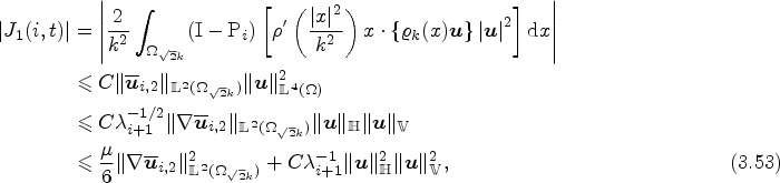
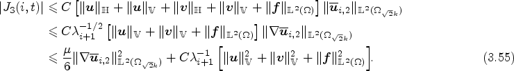
Next, we estimate each term of (3.52) as follows: Using integration by parts, divergence free condition of $u$ , (3.46) (assuming $λ_{i} ⩾ 1$ ), Hölder’s, Ladyzhenskaya’s and Young’s inequalities, we find

\begin{aligned} | J_{1} (i, t) | & = | \frac{2}{k^{2}} \int_{Ω_{\sqrt{2} k}} (I - P_{i}) [ρ^{'} (\frac{| x |^{2}}{k^{2}}) x \cdot {ϱ_{k} (x) u} {| u |}^{2}] d x | \\ ⩽ C ‖ {\bar{u}}_{i, 2} ‖_{L^{2} (Ω_{\sqrt{2} k})} ‖ u ‖_{L^{4} (Ω)}^{2} \\ ⩽ C λ_{i + 1}^{- 1 / 2} ‖ \nabla {\bar{u}}_{i, 2} ‖_{L^{2} (Ω_{\sqrt{2} k})} ‖ u ‖_{H} ‖ u ‖_{V} \\ ⩽ \frac{μ}{6} ‖ \nabla {\bar{u}}_{i, 2} ‖_{L^{2} (Ω_{\sqrt{2} k})}^{2} + C λ_{i + 1}^{- 1} ‖ u ‖_{H}^{2} ‖ u ‖_{V}^{2}, \end{aligned}

(3.53)

\begin{aligned} | J_{2} (i, t) | & = | \int_{Ω_{\sqrt{2} k}} (I - P_{i}) [\nabla p {ϱ_{k} (x)}^{2} u] d x | \\ = \frac{2}{k^{2}} | \int_{Ω_{\sqrt{2} k}} (I - P_{i}) [ρ^{'} (\frac{| x |^{2}}{k^{2}}) (x \cdot ϱ_{k} (x) u) p] d x | \\ ⩽ C ‖ p ‖_{L^{2} (Ω)} ‖ {\bar{u}}_{i, 2} ‖_{L^{2} (Ω_{\sqrt{2} k})} \\ ⩽ C λ_{i + 1}^{- 1 / 2} ‖ u ‖_{L^{4} (Ω)}^{2} ‖ \nabla {\bar{u}}_{i, 2} ‖_{L^{2} (Ω_{\sqrt{2} k})} + C λ_{i + 1}^{- 1 / 2} ‖ f ‖_{L^{2} (Ω)} ‖ \nabla {\bar{u}}_{i, 2} ‖_{L^{2} (Ω_{\sqrt{2} k})} \\ ⩽ \frac{μ}{6} ‖ \nabla {\bar{u}}_{i, 2} ‖_{L^{2} (Ω_{\sqrt{2} k})}^{2} + C λ_{i + 1}^{- 1} [‖ u ‖_{H}^{2} ‖ u ‖_{V}^{2} + ‖ f ‖_{L^{2} (Ω)}^{2}], \end{aligned}

(3.54)

\begin{aligned} | J_{3} (i, t) | & ⩽ C [‖ u ‖_{H} + ‖ u ‖_{V} + ‖ v ‖_{H} + ‖ v ‖_{V} + ‖ f ‖_{L^{2} (Ω)}] ‖ {\bar{u}}_{i, 2} ‖_{L^{2} (Ω_{\sqrt{2} k})} \\ ⩽ C λ_{i + 1}^{- 1 / 2} [‖ u ‖_{V} + ‖ v ‖_{V} + ‖ f ‖_{L^{2} (Ω)}] ‖ \nabla {\bar{u}}_{i, 2} ‖_{L^{2} (Ω_{\sqrt{2} k})} \\ ⩽ \frac{μ}{6} ‖ \nabla {\bar{u}}_{i, 2} ‖_{L^{2} (Ω_{\sqrt{2} k})}^{2} + C λ_{i + 1}^{- 1} [‖ u ‖_{V}^{2} + ‖ v ‖_{V}^{2} + ‖ f ‖_{L^{2} (Ω)}^{2}] . \end{aligned}

(3.55)

Combining (3.52)–(3.55), we infer for

α = min {\frac{3 μ λ}{4}, 2 δ}

\begin{aligned} \frac{d}{d t} [‖ {\bar{u}}_{i, 2} ‖_{L^{2} (Ω_{\sqrt{2} k})}^{2} + γ ‖ \nabla {\bar{v}}_{i, 2} ‖_{L^{2} (Ω_{\sqrt{2} k})}^{2}] + α [‖ {\bar{u}}_{i, 2} ‖_{L^{2} (Ω_{\sqrt{2} k})}^{2} + γ ‖ \nabla {\bar{v}}_{i, 2} ‖_{L^{2} (Ω_{\sqrt{2} k})}^{2}] \\ ⩽ \frac{d}{d t} ‖ {\bar{u}}_{i, 2} ‖_{L^{2} (Ω_{\sqrt{2} k})}^{2} + γ \frac{d}{d t} ‖ \nabla {\bar{v}}_{i, 2} ‖_{L^{2} (Ω_{\sqrt{2} k})}^{2} + \frac{3 μ λ}{4} ‖ {\bar{u}}_{i, 2} ‖_{L^{2} (Ω_{\sqrt{2} k})}^{2} + 2 δ γ ‖ \nabla {\bar{v}}_{i, 2} ‖_{L^{2} (Ω_{\sqrt{2} k})}^{2} \\ ⩽ \frac{d}{d t} ‖ {\bar{u}}_{i, 2} ‖_{L^{2} (Ω_{\sqrt{2} k})}^{2} + γ \frac{d}{d t} ‖ \nabla {\bar{v}}_{i, 2} ‖_{L^{2} (Ω_{\sqrt{2} k})}^{2} + μ ‖ \nabla {\bar{u}}_{i, 2} ‖_{L^{2} (Ω_{\sqrt{2} k})}^{2} + 2 δ γ ‖ \nabla {\bar{v}}_{i, 2} ‖_{L^{2} (Ω_{\sqrt{2} k})}^{2} \\ ⩽ C λ_{i + 1}^{- 1} [‖ u ‖_{H}^{2} ‖ u ‖_{V}^{2} + ‖ u ‖_{V}^{2} + ‖ v ‖_{V}^{2} + ‖ f ‖_{L^{2} (Ω)}^{2}] . \end{aligned}

(3.56)

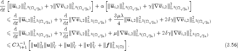
Applying variation of constants formula to (3.56), we find

\begin{aligned} {‖ {\bar{u}}_{i, 2} (t) ‖}_{L^{2} (Ω_{\sqrt{2} k})}^{2} + γ {‖ \nabla {\bar{v}}_{i, 2} (t) ‖}_{L^{2} (Ω_{\sqrt{2} k})}^{2} \\ ⩽ {‖ {\bar{u}}_{i, 2} (t_{B}) ‖}_{L^{2} (Ω_{\sqrt{2} k})}^{2} + γ {‖ \nabla {\bar{v}}_{i, 2} (t_{B}) ‖}_{L^{2} (Ω_{\sqrt{2} k})}^{2} \\ + C λ_{i + 1}^{- 1} \int_{t_{B}}^{t} e^{- α (t - s)} [{‖ u (s) ‖}_{H}^{2} {‖ u (s) ‖}_{V}^{2} + {‖ u (s) ‖}_{V}^{2} + {‖ v (s) ‖}_{V}^{2} + ‖ f ‖_{L^{2} (Ω)}^{2}] \\ ⩽ {‖ {\bar{u}}_{i, 2} (t_{B}) ‖}_{L^{2} (Ω_{\sqrt{2} k})}^{2} + γ {‖ \nabla {\bar{v}}_{i, 2} (t_{B}) ‖}_{L^{2} (Ω_{\sqrt{2} k})}^{2} + C λ_{i + 1}^{- 1} \\ \to 0 as i \to \infty, \end{aligned}

(3.57)

for

t ⩾ t_{B}

, where we have used (3.24). Hence, from (3.57), we conclude that for any

ε > 0

, there exists a

i_{0} \in N

such that

\begin{aligned} {| | (I - P_{i}) \bar{u} (t) | |}_{L^{2} (Ω_{\sqrt{2} k})}^{2} + γ ‖ (I - P_{i}) \nabla \bar{v} (t) ‖_{L^{2} (Ω_{\sqrt{2} k})}^{2} ⩽ ε, \end{aligned}

(3.58)

for all

i ⩾ i_{0}

and

t ⩾ t_{B}

. This completes the proof.

In the following proposition, we demonstrate the asymptotic compactness of the semigroup ${S (t)}_{t ⩾ 0}$ associated with the system (3.2) using the results obtained in Lemmas 3.5 and 3.6.

Proposition 3.7.

The semigroup ${S (t)}_{t ⩾ 0}$ is asymptotically compact in $X$ .

Proof.

It is enough to show that for arbitrary sequences $τ_{n} \to + \infty$ and ${U_{0, n}} \subset X$ , the sequence

\begin{aligned} U_{n} = S (t_{n}) U_{0, n} \end{aligned}

is pre-compact in

X

. Let

E_{N} = {U_{n} : n ⩾ N}

N = 1, 2, \dots

. In order to prove the pre-compactness of the sequence

U_{n}

, we need to show that the Kuratowski measure

κ_{H} (E_{N}) \to 0

and

N \to + \infty

, (cf. Lemma 2.4).

Since, $t_{n} \to \infty$ , there exists $N \in N$ such that $t_{n} ⩾ t_{B}$ for all $n ⩾ N$ . For each $η > 0$ , by Lemma 3.5, there exists $K_{0} ⩾ 1$ such that

\begin{aligned} {‖ ρ (\frac{| \cdot |^{2}}{k^{2}}) U_{n} ‖}_{L^{2} {(Ω}_{K}^{c}) \times H_{0}^{1} {(Ω}_{K}^{c})} ⩽ \frac{η}{2}, \end{aligned}

(3.59)

for all

n ⩾ N

and for all

K ⩾ K_{0}

. Let us fix

K ⩾ K_{0}

. By Lemma 3.6, there exists

i_{0} \in N

such that

\begin{aligned} {| | (I - P_{i}) (ϱ_{K} U_{n}) | |}_{L^{2} (Ω_{\sqrt{2} K}) \times H_{0}^{1} (Ω_{\sqrt{2} K})} ⩽ \frac{η}{2}, \end{aligned}

(3.60)

for all

n ⩾ N

and for all

i ⩾ i_{0}

Now, the inequality (3.24) provides us that the set $E_{N}$ is bounded in $X$ which further implies that the set ${ϱ_{K} U_{n} : n ⩾ N}$ is bounded in $L^{2} (Ω_{\sqrt{2} K}) \times H_{0}^{1} (Ω_{\sqrt{2} K})$ . Hence, by the finite-dimensional range of $P_{i}$ , $P_{i} ({ϱ_{K} U_{n} : n ⩾ N})$ is pre-compact in $L^{2} (Ω_{\sqrt{2} K}) \times H_{0}^{1} (Ω_{\sqrt{2} K})$ , from which we conclude that

\begin{aligned} κ_{L^{2} (Ω_{\sqrt{2} K}) \times H_{0}^{1} (Ω_{\sqrt{2} K})} (P_{i} ({ϱ_{K} U_{n} : n ⩾ N})) = 0. \end{aligned}

(3.61)

It follows from (3.60)–(3.61) and [39, Theorem 1.4] that

\begin{aligned} κ_{L^{2} (Ω_{\sqrt{2} K}) \times H_{0}^{1} (Ω_{\sqrt{2} K})} ({ϱ_{K} U_{n} : n ⩾ N}) \\ ⩽ κ_{L^{2} (Ω_{\sqrt{2} K}) \times H_{0}^{1} (Ω_{\sqrt{2} K})} (P_{i} ({ϱ_{K} U_{n} : n ⩾ N})) \\ + κ_{L^{2} (Ω_{\sqrt{2} K}) \times H_{0}^{1} (Ω_{\sqrt{2} K})} ((I - P_{i}) ({ϱ_{K} U_{n} : n ⩾ N})) \\ ⩽ \frac{η}{2} . \end{aligned}

(3.62)

We infer from (3.59) and (3.62) that

\begin{aligned} κ_{X} (E_{N}) ⩽ κ_{L^{2} (Ω_{\sqrt{2} K}) \times H_{0}^{1} (Ω_{\sqrt{2} K})} (ϱ_{K} E_{N}) + κ_{L^{2} (Ω_{K}^{c}) \times H_{0}^{1} (Ω_{K}^{c})} (ρ (\frac{| \cdot |^{2}}{k^{2}}) E_{N}) ⩽ η, \end{aligned}

which shows that

S (\cdot)

is asymptotically compact in

X

. This completes the proof.

Using the existence of absorbing set, the asymptotic compactness of the semigroup ${S (t)}_{t ⩾ 0}$ and Theorem 3.1, we have the following result immediately:

Theorem 3.8.

Let Ω satisfy Hypothesis 1.1. Assume that $μ > 0$ and $f \in L^{2} (Ω)$ . Then the semigroup ${S (t)}_{t ⩾ 0}$ associated with the system (3.2) possesses a global attractor $A$ in $X$ , that is, a compact invariant set in $X$ , which attracts all bounded sets in $X$ . Moreover, $A$ is connected in $X$ and is maximal for the inclusion relation among all the functional invariant sets bounded in $X$ .

Since the system (2.5) is equivalent to the system (3.1) which is a particular case of the system (3.2) with $v_{0} = 0$ , we provide the following result on the existence of global attractors for the system (2.5). Corollary 3.9.

Let Ω satisfy Hypothesis 1.1. Assume that $μ > 0$ and $f \in L^{2} (Ω)$ . Then the semigroup ${S (t)}_{t ⩾ 0}$ associated with the Oldroyd system (2.5) possesses a global attractor $A_{H}$ in $H$ .

4. Dimension of the attractor

In this section, we analyze the dimension of the global attractor $A$ obtained in Section 3. We estimate the bounds for the Hausdorff as well as fractal dimensions of the global attractor $A$ .

Let $U_{0} \in X$ and $U (t) = S (t) U_{0}$ , for $t ⩾ 0$ be the unique weak solution of the system (3.2). The linearized flow around $U = (u, v)^{⊤}$ is given by the following system:

\begin{aligned} {\begin{cases} \frac{d}{d t} ξ (t) + μ A ξ (t) + γ A ζ (t) + B (ξ (t), u (t)) + B (u (t), ξ (t)) = 0, t \in (0, T), \\ \frac{d ζ (t)}{d t} + δ ζ (t) - ξ (t) = 0, t \in (0, T), \\ ξ (0) = ξ_{0}, ζ (0) = ζ_{0} . \end{cases} \end{aligned}

(4.1)

As in the case of nonlinear problem, one can show that there exists a unique solution

W = (ξ, ζ)^{⊤} \in L^{\infty} (0, T; H) \cap L^{2} (0, T; V) \times L^{\infty} (0, T; V)

, for all

T > 0

. Furthermore,

W_{t} = (ξ_{t}, ζ_{t})^{⊤} \in L^{2} (0, T; V^{'}) \times L^{2} (0, T; V)

and

W \in C ([0, T]; H) \times C ([0, T]; V)

, for all

T > 0

. We define a map

Λ (t; U_{0}) : X \to X

by setting

Λ (t; U_{0}) W_{0} = W (t)

, where

W_{0} = (ξ_{0}, ζ_{0})

. In the next lemma, we show that the map

Λ (t; U_{0})

is bounded and the semigroup

{S (t)}_{t ⩾ 0}

is uniformly differentiable on

A

, that is,

\begin{aligned} lim_{ε \to 0} sup_{\begin{matrix} U_{0}, V_{0} \in A \\ 0 < ‖ U_{0} - V_{0} ‖_{X} ⩽ ε \end{matrix}} \frac{‖ S (t) V_{0} - S (t) U_{0} - Λ (t; U_{0}) (V_{0} - U_{0}) ‖_{X}}{‖ V_{0} - U_{0} ‖_{X}} = 0. \end{aligned}

(4.2)

Lemma 4.1.

Let $U_{0}$ and $V_{0}$ be two members of $X$ . Then there exists a constant $K = K (‖ U_{0} ‖_{X}, ‖ V_{0} ‖_{X})$ such that

\begin{aligned} \frac{‖ S (t) V_{0} - S (t) U_{0} - Λ (t; U_{0}) (V_{0} - U_{0}) ‖_{X}}{‖ V_{0} - U_{0} ‖_{X}} ⩽ K ‖ V_{0} - U_{0} ‖_{X}, \end{aligned}

(4.3)

where the linear operator

Λ (t; U_{0}) : X \to X

, for

t > 0

is the solution operator of the problem ( 4.1 ) with

U (t) = (u_{1} (t), v_{1} (t))^{⊤} = S (t) U_{0}

. In other words, for every

t > 0

, the map

S (t) U_{0}

, as a map

S (t) : X \to X

is Fréchet differentiable with respect to the initial data, and its Fréchet derivative

D_{U_{0}} (S (t) U_{0}) W_{0} = Λ (t; U_{0}) W_{0}

. Moreover, ( 4.2 ) is satisfied.

Proof.

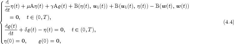
For $U (t) = (u_{1} (t), v_{1} (t))^{⊤}$ and $V (t) = (u_{2} (t), v_{2} (t))^{⊤}$ , let us define

\begin{aligned} Ψ (t) = (\begin{matrix} η (t) \\ ϱ (t) \end{matrix}) := (\begin{matrix} u_{1} (t) - u_{2} (t) - ξ (t) \\ v_{1} (t) - v_{2} (t) - ζ (t) \end{matrix}) = S (t) (\begin{matrix} u_{0}^{1} - u_{0}^{2} \\ v_{0}^{1} - v_{0}^{2} \end{matrix}) - (\begin{matrix} ξ (t) \\ ζ (t) \end{matrix}), \end{aligned}

and

Φ (t) = (\begin{matrix} ξ (t) \\ ζ (t) \end{matrix})

. Then

(η (t), ϱ (t))^{⊤}

satisfies:

\begin{aligned} {\begin{cases} \frac{d}{d t} η (t) + μ A η (t) + γ A ϱ (t) + B (η (t), u_{1} (t)) + B (u_{1} (t), η (t)) - B (w (t), w (t)) \\ = 0, t \in (0, T), \\ \frac{d ϱ (t)}{d t} + δ ϱ (t) - η (t) = 0, t \in (0, T), \\ η (0) = 0, ϱ (0) = 0, \end{cases} \end{aligned}

(4.4)

where

w (t) = u_{1} (t) - u_{2} (t)

. Let us take the inner product with

η (\cdot)

to the first equation in (4.4) to obtain

\begin{aligned} \frac{1}{2} \frac{d}{d t} {‖ η (t) ‖}_{H}^{2} + μ {‖ η (t) ‖}_{V}^{2} \\ = - γ (\nabla ϱ (t), \nabla η (t)) - b (η (t), u_{1} (t), η (t)) + b (w (t), w (t), η (t)), \end{aligned}

(4.5)

for a.e.

t \in [0, T]

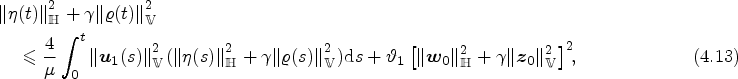
. Next we take the inner product with

γ A ϱ (\cdot)

to the second equation in (4.4) to get

\begin{aligned} \frac{1}{2} \frac{d}{d t} γ ‖ ϱ (t) ‖_{V}^{2} + δ γ ‖ ϱ (t) ‖_{V}^{2} = γ (\nabla η (t), \nabla ϱ (t)), \end{aligned}

(4.6)

for a.e.

t \in [0, T]

. Adding (4.5) and (4.6), we arrive at

\begin{aligned} \frac{1}{2} \frac{d}{d t} ({‖ η (t) ‖}_{H}^{2} + γ {‖ ϱ (t) ‖}_{V}^{2}) + μ {‖ η (t) ‖}_{V}^{2} + γ δ {‖ ϱ (t) ‖}_{V}^{2} \\ = - b (η (t), u_{1} (t), η (t)) + b (w (t), w (t), η (t)), \end{aligned}

(4.7)

for a.e.

t \in [0, T]

. We estimate

| b (η, u_{1}, η) |

and

| b (w, w, η) |

using Hölder’s, Ladyzhenskaya’s and Young’s inequalities as

\begin{aligned} | b (η, u_{1}, η) | & ⩽ ‖ u_{1} ‖_{V} ‖ η ‖_{L^{4}}^{2} ⩽ \sqrt{2} ‖ u_{1} ‖_{V} ‖ η ‖_{H} ‖ η ‖_{V} ⩽ \frac{μ}{4} ‖ η ‖_{V}^{2} + \frac{2}{μ} ‖ u_{1} ‖_{V}^{2} ‖ η ‖_{H}^{2}, \end{aligned}

(4.8)

\begin{aligned} | b (w, w, η) | & = | b (w, η, w) | \\ ⩽ ‖ η ‖_{V} ‖ w ‖_{L^{4}}^{2} ⩽ \sqrt{2} ‖ η ‖_{V} ‖ w ‖_{H} ‖ w ‖_{V} ⩽ \frac{μ}{4} ‖ η ‖_{V}^{2} + \frac{2}{μ} ‖ w ‖_{H}^{2} ‖ w ‖_{V}^{2} . \end{aligned}

(4.9)

Combining (4.8) and (4.9), and applying it in (4.7), we find

\begin{aligned} \frac{d}{d t} ({‖ η (t) ‖}_{H}^{2} + γ {‖ ϱ (t) ‖}_{V}^{2}) + μ {‖ η (t) ‖}_{V}^{2} + 2 γ δ {‖ ϱ (t) ‖}_{V}^{2} \\ ⩽ \frac{4}{μ} {‖ u_{1} (t) ‖}_{V}^{2} {‖ η (t) ‖}_{H}^{2} + \frac{4}{μ} {‖ w (t) ‖}_{H}^{2} {‖ w (t) ‖}_{V}^{2}, \end{aligned}

(4.10)

for a.e.

t \in [0, T]

. Remember that

(w (t), z (t))^{⊤} = (u_{1} (t) - u_{2} (t), v_{1} (t) - v_{2} (t))^{⊤} = S (t) U_{0} - S (t) V_{0}

satisfies (see (3.19)):

\begin{aligned} {‖ w (t) ‖}_{H}^{2} + μ \int_{0}^{t} {‖ w (s) ‖}_{V}^{2} d s \\ ⩽ [‖ w_{0} ‖_{H}^{2} + γ ‖ z_{0} ‖_{V}^{2}] \exp {\frac{2}{μ^{2}} (‖ u_{0} ‖_{H}^{2} + γ ‖ v_{0} ‖_{V}^{2} + \frac{t}{μ} ‖ f ‖_{H^{- 1} (Ω)}^{2})}, \end{aligned}

(4.11)

for all

t \in [0, T]

. Using (4.11) in (4.10) and then integrating from 0 to t, we find

\begin{aligned} {‖ η (t) ‖}_{H}^{2} + γ {‖ ϱ (t) ‖}_{V}^{2} + μ \int_{0}^{t} {‖ η (s) ‖}_{V}^{2} d s + 2 γ δ \int_{0}^{t} {‖ ϱ (s) ‖}_{V}^{2} d s \\ ⩽ \frac{4}{μ} \int_{0}^{t} {‖ u_{1} (s) ‖}_{V}^{2} {‖ η (s) ‖}_{H}^{2} d s + \frac{4}{μ} sup_{s \in [0, t]} {‖ w (s) ‖}_{H}^{2} \int_{0}^{t} {‖ w (s) ‖}_{V}^{2} d s \\ ⩽ \frac{4}{μ} \int_{0}^{t} {‖ u_{1} (s) ‖}_{V}^{2} {‖ η (s) ‖}_{H}^{2} d s + \frac{4}{μ^{2}} {[‖ w_{0} ‖_{H}^{2} + γ ‖ z_{0} ‖_{V}^{2}]}^{2} \\ \times \exp {\frac{2}{μ^{2}} (‖ u_{0} ‖_{H}^{2} + γ ‖ v_{0} ‖_{V}^{2} + \frac{t}{μ} ‖ f ‖_{H^{- 1} (Ω)}^{2})}, \end{aligned}

(4.12)

for all

t \in [0, T]

. Thus, from (4.12), we infer that

\begin{aligned} {‖ η (t) ‖}_{H}^{2} + γ {‖ ϱ (t) ‖}_{V}^{2} \\ ⩽ \frac{4}{μ} \int_{0}^{t} {‖ u_{1} (s) ‖}_{V}^{2} ({‖ η (s) ‖}_{H}^{2} + γ {‖ ϱ (s) ‖}_{V}^{2}) d s + ϑ_{1} {[‖ w_{0} ‖_{H}^{2} + γ ‖ z_{0} ‖_{V}^{2}]}^{2}, \end{aligned}

(4.13)

for all

t \in [0, T]

, where

\begin{aligned} ϑ_{1} = \frac{4}{μ^{2}} \exp {\frac{2}{μ^{2}} (‖ u_{0} ‖_{H}^{2} + γ ‖ v_{0} ‖_{V}^{2} + \frac{T}{μ} ‖ f ‖_{H^{- 1} (Ω)}^{2})} . \end{aligned}

An application of Gronwall’s inequality in (4.13) yields

\begin{aligned} {‖ η (t) ‖}_{H}^{2} + γ {‖ ϱ (t) ‖}_{V}^{2} ⩽ ϑ_{1} {[‖ w_{0} ‖_{H}^{2} + γ ‖ z_{0} ‖_{V}^{2}]}^{2} e^{\frac{4 M_{1}^{2} T}{μ}}, \end{aligned}

that is,

\begin{aligned} {‖ Ψ (t) ‖}_{X}^{2} ⩽ \frac{1}{κ} ϑ_{2} ‖ W_{0} ‖_{X}^{4}, \end{aligned}

where

ϑ_{2} = ϑ_{1} e^{\frac{4 M_{1} T}{μ}}

and

W_{0} = U_{0} - V_{0}

. Thus, by the definition of

Ψ (t)

, it is immediate that

\begin{aligned} \frac{‖ U (t) - V (t) - Φ (t) ‖_{X}}{‖ U_{0} - V_{0} ‖_{X}} ⩽ \sqrt{\frac{ϑ_{2}}{κ}} ‖ U_{0} - V_{0} ‖_{X}, \end{aligned}

(4.14)

and hence the differentiability of

S (t)

with respect to the initial data as well as (4.2) and (4.3) follows.

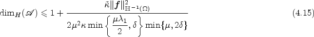
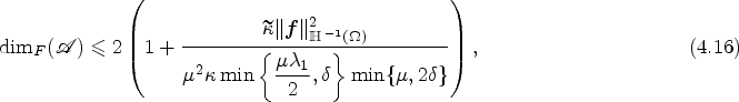
In the next theorem, we show that the global attractor obtained in Theorem 3.8 has finite Hausdorff and fractal dimensions, and we find their bounds also.

Theorem 4.2.

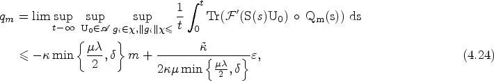
The global attractor obtained in Theorem 3.8 has finite Hausdorff and fractal dimensions, which can be estimated as

\begin{aligned} \dim_{H} (A) ⩽ 1 + \frac{\tilde{κ} ‖ f ‖_{H^{- 1} (Ω)}^{2}}{2 μ^{2} κ min {\frac{μ λ_{1}}{2}, δ} min {μ, 2 δ}} \end{aligned}

(4.15)

and

\begin{aligned} \dim_{F} (A) ⩽ 2 (1 + \frac{\tilde{κ} ‖ f ‖_{H^{- 1} (Ω)}^{2}}{μ^{2} κ min {\frac{μ λ_{1}}{2}, δ} min {μ, 2 δ}}), \end{aligned}

(4.16)

for some absolute constant

\tilde{κ}

Proof.

We can rewrite the system (4.1) as

\begin{aligned} \frac{dW}{d t} = F^{'} (U) W = (\begin{matrix} - [μ A ξ + γ A ζ + B (ξ, u) + B (u, ξ)] \\ - [δ ζ - ξ] \end{matrix}), where W = (\begin{matrix} ξ \\ ζ \end{matrix}), \end{aligned}

(4.17)

with

W (0) = (\begin{matrix} ξ_{0} \\ ζ_{0} \end{matrix})

. We define the numbers

q_{m}

m \in N

\begin{aligned} q_{m} & = \underset{t \to \infty}{lim sup} sup_{U_{0} \in A} sup_{\begin{matrix} ϱ_{i} \in χ, ‖ ϱ_{i} ‖ χ ⩽ 1 \\ i = 1, \dots, n \end{matrix}} \frac{1}{t} \int_{0}^{t} Tr (F^{'} (S (s) U_{0}) \circ Q_{m} (s)) d s \end{aligned}

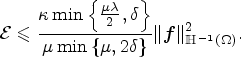
where $Q_{m} (s) = Q_{m} (s; U_{0}, ϱ_{1}, \dots, ϱ_{m})$ is the orthogonal projector of $X$ onto the space spanned by ${Λ (t; U_{0}) ϱ_{1}, \dots, Λ (t; U_{0}) ϱ_{m}}$ . From [48, Section V.3.4] (see Proposition V.2.1 and Theorem V.3.3), we infer that if $q_{m} < 0$ , for some $m \in N$ , then the global attractor $A$ has finite Hausdorff and fractal dimensions estimated respectively as

\begin{aligned} \dim_{H} (A) ⩽ m, \end{aligned}

(4.18)

\begin{aligned} \dim_{F} (A) ⩽ m (1 + max_{1 ⩽ j ⩽ m} \frac{{(q_{j})}_{+}}{| q_{m} |}) . \end{aligned}

(4.19)

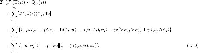
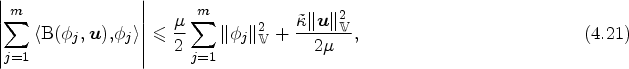
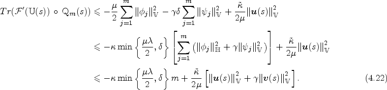
Our next aim is to estimate the number

q_{m}

. Let

U_{0} \in A

ϱ_{1}, \dots, ϱ_{m} \in X

and set

U (t) = S (t) U_{0}

and

W_{j} (t) = Λ (t; U_{0}) ϱ_{j}

t ⩾ 0

and

1 ⩽ j ⩽ m

. Let us consider

{Φ_{1} (t), \dots, Φ_{m} (t)} = {(\begin{matrix} ϕ_{1} (t) \\ ψ_{1} (t) \end{matrix}), \dots, (\begin{matrix} ϕ_{m} (t) \\ ψ_{m} (t) \end{matrix})}

as an orthonormal basis in

X

for

span {W_{1} (t), \dots, W_{m} (t)}

. Note that

‖ ϕ_{j} ‖_{H}^{2} + γ ‖ ψ_{j} ‖_{V}^{2} = 1

, for all

1 ⩽ j ⩽ m

. Since

W_{j} \in L^{2} (0, T; V) \times L^{\infty} (0, T; V)

, we know that

W_{j} (t) \in V \times V

, a.e.

t \in (0, T)

. By the Gram–Schmidt orthogonalization process, we can assume that

Φ_{j} (t) \in V \times V

. Then, one can see that

\begin{aligned} T r (F^{'} (U (s)) \circ Q_{m} (s)) \\ = \sum_{j = 1}^{m} [[F^{'} (U (s)) Φ_{j}, Φ_{j}]] \\ = \sum_{j = 1}^{m} {⟨ - μ A ϕ_{j} - γ A ψ_{j} - B (ϕ_{j}, u) - B (u, ϕ_{j}), ϕ_{j} ⟩ - γ δ (\nabla ψ_{j}, \nabla ψ_{j}) + γ ⟨ ϕ_{j}, A ψ_{j} ⟩} \\ = \sum_{j = 1}^{m} {- μ ‖ ϕ_{j} ‖_{V}^{2} - γ δ ‖ ψ_{j} ‖_{V}^{2} - ⟨ B (ϕ_{j}, u), ϕ_{j} ⟩} . \end{aligned}

(4.20)

Calculating similarly as in [42, p. 82], we find

\begin{aligned} | \sum_{j = 1}^{m} ⟨ B (ϕ_{j}, u), ϕ_{j} ⟩ | ⩽ \frac{μ}{2} \sum_{j = 1}^{m} ‖ ϕ_{j} ‖_{V}^{2} + \frac{\tilde{κ} ‖ u ‖_{V}^{2}}{2 μ}, \end{aligned}

(4.21)

for an absolute constant

\tilde{κ}

. Thus, from (4.20), we infer

\begin{aligned} T r (F^{'} (U (s)) \circ Q_{m} (s)) & ⩽ - \frac{μ}{2} \sum_{j = 1}^{m} ‖ ϕ_{j} ‖_{V}^{2} - γ δ \sum_{j = 1}^{m} ‖ ψ_{j} ‖_{V}^{2} + \frac{\tilde{κ}}{2 μ} {‖ u (s) ‖}_{V}^{2} \\ ⩽ - κ min {\frac{μ λ}{2}, δ} [\sum_{j = 1}^{m} (‖ ϕ_{j} ‖_{H}^{2} + γ ‖ ψ_{j} ‖_{V}^{2})] + \frac{\tilde{κ}}{2 μ} {‖ u (s) ‖}_{V}^{2} \\ ⩽ - κ min {\frac{μ λ}{2}, δ} m + \frac{\tilde{κ}}{2 μ} [{‖ u (s) ‖}_{V}^{2} + γ {‖ v (s) ‖}_{V}^{2}] . \end{aligned}

(4.22)

Let us define the energy dissipation flux as

\begin{aligned} E = κ min {\frac{μ λ}{2}, δ} \underset{t \to \infty}{\lim \sup} sup_{U_{0} \in A} \frac{1}{t} \int_{0}^{t} ‖ S (s) U_{0} ‖_{V \times V}^{2} d s . \end{aligned}

(4.23)

Note that the energy dissipation flux

E

is finite due to the estimate (3.6) and

\begin{aligned} E ⩽ \frac{κ min {\frac{μ λ}{2}, δ}}{μ min {μ, 2 δ}} ‖ f ‖_{H^{- 1} (Ω)}^{2} . \end{aligned}

Then, from (4.22), we have

\begin{aligned} q_{m} & = lim sup_{t - \infty} sup_{U_{0} \in A} sup_{g_{i} \in χ, ‖ g_{i} ‖ χ ⩽} \frac{1}{t} \int_{0}^{t} Tr (F^{'} (S (s) U_{0}) \circ Q_{m} (s)) ds \\ ⩽ - κ min {\frac{μ λ}{2}, δ} m + \frac{\tilde{κ}}{2 κ μ min {\frac{μ λ}{2}, δ}} ε, \end{aligned}

(4.24)

for all

m \in N

. Hence, if

m^{'} \in N

is defined by

\begin{aligned} m^{'} - 1 ⩽ \frac{\tilde{κ}}{2 κ^{2} μ min {\frac{μ λ}{2}, δ}^{2}} E < m^{'}, \end{aligned}

then

q_{m^{'}} < 0

and thus from (4.18), we find

\begin{aligned} \dim_{H} (A) ⩽ m^{'} ⩽ 1 + \frac{\tilde{κ}}{2 κ^{2} μ min {\frac{μ λ}{2}, δ}^{2}} E ⩽ 1 + \frac{\tilde{κ} ‖ f ‖_{H^{- 1} (Ω)}^{2}}{2 μ^{2} κ min {\frac{μ λ}{2}, δ} min {μ, 2 δ}} . \end{aligned}

(4.25)

Furthermore, if

m^{″} \in N

is defined by

\begin{aligned} m^{″} - 1 < \frac{\tilde{κ}}{μ κ^{2} min {\frac{μ λ}{2}, δ}^{2}} E ⩽ m^{″}, \end{aligned}

then using [48, Lemma VI.2.2], we have

\begin{aligned} q_{m^{″}} < 0 and \frac{{(q_{j})}_{+}}{| q_{m^{″}} |} ⩽ 1, for all j = 1, \dots, m^{″} . \end{aligned}

(4.26)

Hence from (4.19), we obtain

\begin{aligned} \dim_{F} (A) ⩽ 2 m^{″} ⩽ 2 (1 + \frac{\tilde{κ}}{μ κ^{2} min {\frac{μ λ}{2}, δ}^{2}} E) ⩽ 2 (1 + \frac{\tilde{κ} ‖ f ‖_{H^{- 1} (Ω)}^{2}}{μ^{2} κ min {\frac{μ λ}{2}, δ} min {μ, 2 δ}}), \end{aligned}

(4.27)

which completes the proof.

Footnotes

Acknowledgements

The authors would like to thank the Department of Science and Technology (DST) Science & Engineering Research Board (SERB), India for a MATRICS grant (MTR/2021/000066). In December 2023, the first author visited the Indian Institute of Technology Roorkee in Roorkee, India, and was greatly assisted by their gracious hospitality in completing this work.

Conflict of interest

The authors have declared no conflict of interest.

Declaration of interests

The authors declare that they have no known competing financial interests or personal relationships that could have appeared to influence the work reported in this paper.

References

Abergel

, Attractor for a Navier–Stokes flow in an unbounded domain, Math. Mod. Num. Anal. 23 (1989), 359–370. doi:10.1051/m2an/1989230303591.

Abergel

, Existence and finite dimensionality of the global attractor for evolution equations on unbounded domains, J. Diff. Equ. 83 (1990), 85–108. doi:10.1016/0022-0396(90)90070-6.

Agranovich

Y.Y.

Sobolevskii

P.E.

, Investigation of viscoelastic fluid mathematical model, RAC. Ukranian SSR., Ser. A 10 (1989), 71–73.

Agranovich

Y.Y.

Sobolevskii

P.E.

, The motion of non-linear viscoelastic fluid, RAC. USSR 314 (1990), 231–233.

Agranovich

Y.Y.

Sobolevskii

P.E.

, Motion of non-linear viscoelastic fluid, Nonlinear Analysis 32 (1998), 755–760. doi:10.1016/S0362-546X(97)00519-1.

Babin

A.V.

, The attractor of a Navier–Stokes system in an unbounded channel-like domain, J. Dyn. Differ. Equ. 4 (1992), 555–584. doi:10.1007/BF01048260.

Babin

A.V.

Vishik

M.I.

, Attractors of partial differential equations in an unbounded domain, Proc. R. Soc. Edin. A 116 (1990), 221–243. doi:10.1017/S0308210500031498.

Ball

J.M.

, Continuity properties of global attractors of generalized semiflows and the Navier–Stokes equations, J. Nonlin. Sci. 7 (1997), 475–502. doi:10.1007/s003329900037.

Barbu

Sritharan

S.S.

, Navier–Stokes equation with hereditary viscosity, Zeitschrift für angewandte Mathematik und Physik 54 (2003), 1–13. doi:10.1007/PL00012626.

10.

Cannon

J.R.

Ewing

R.E.

Lin

, A modified nonlinear Galerkin method for the viscoelastic fluid motion equations, International Journal of Engineering Science 37 (1999), 1643–1662. doi:10.1016/S0020-7225(98)00142-6.

11.

Caraballo

Real

, Attractors for 2D-Navier–Stokes models with delays, J. Differential Equations 205 (2004), 271–297. doi:10.1016/j.jde.2004.04.012.

12.

Chepyzhov

V.V.

Conti

Pata

, Averaging of equations of viscoelasticity with singularly oscillating external forces, Journal de Mathématiques Pures et Appliquées 108 (2017), 841–868. doi:10.1016/j.matpur.2017.05.007.

13.

Constantin

Foias

, Global Lyapunov exponents, Kaplan–Yorke formulas and the dimension of the attractors for 2D Navier–Stokes equations, Commun. Pure Appl. Math. 38 (1985), 1–27. doi:10.1002/cpa.3160380102.

14.

Constantin

Foias

, Navier–Stokes Equations, Chicago Lectures in Mathematical Series, 1989.

15.

Constantin

Foias

Temam

, Attractors Representing Turbulent Flows, Memoirs of the American Mathematical Society, Vol. 53, 1985.

16.

Dafermos

C.M.

, Asymptotic stability in viscoelasticity, Arch. Rational Mech. Anal. 37 (1970), 297–308. doi:10.1007/BF00251609.

17.

Foias

Manley

Rosa

Temam

, Navier–Stokes Equations and Turbulence, Cambridge University Press, 2001.

18.

Heywood

J.G.

, The Navier–Stokes equations: On the existence, regularity and decay of solutions, Ind. Univ. Math. J. 29 (1980), 639–681. doi:10.1512/iumj.1980.29.29048.

19.

, The

H^{1}

-compact global attractor for the solutions to the Navier–Stokes equations in two-dimensional unbounded domains, Nonlinearity 13 (2000), 1227–1238. doi:10.1088/0951-7715/13/4/313.

20.

Karazeeva

N.A.

, Initial boundary value problems for linear viscoelastic flows generated by integro-differential equations, Journal of Mathematical Sciences 127 (2005), 1869–1874. doi:10.1007/s10958-005-0147-6.

21.

Karazeeva

N.A.

, Asymptotic behavior and attractor of systems governing two-dimensional viscoelastic flows, Journal of Mathematical Sciences 242 (2019), 1–14. doi:10.1007/s10958-019-04463-y.

22.

Karazeeva

N.A.

Kotsiolis

A.A.

Oskolkov

A.P.

, Dynamic system and attractors generated b.y the initial boundary value problems for equations of motion of linear viscoelaztic fluids, Trudy Mat. Inst., Steklov 188 (1990), 60–87.

23.

Karazeeva

N.A.

Kotsiolis

A.A.

Oskolkov

A.P.

, Dynamical systems generated by initial-boundary value problems for equations of motion of linear viscoelastic fluids, Proc. Steklov Inst. Math. 3 (1991), 73–108.

24.

Kinra

Mohan

M.T.

Wang

, Asymptotically autonomous robustness of non-autonomous random attractors for stochastic convective Brinkman–Forchheimer equations on

R^{3}

, Int. Math. Res. Not. IMRN 2024 (2024), 5850–5893. doi:10.1093/imrn/rnad279.

25.

Kotsiolis

A.A.

, Attractors of initial-boundary value problems for equations of motion of Jeffreys–Oldroyd fluids in domains with nonsmooth and smooth boundaries, Zap. Nauchn. Sem. S.-Peterburg. Otdel. Mat. Inst. Steklov. (POMI) 208 (1993), 186–199.

26.

Kotsiolis

A.A.

Oskolkov

A.P.

, On the solvability of fundamental initial-boundary value problem for the motion equations of Oldroyd’s fluid and the behavior of solutions, when

t \to \infty

, Notes of Scientifics of LOMI 150 (1986), 48–52.

27.

Kotsiolis

A.A.

Oskolkov

A.P.

, On a dynamic system generated by equations of motion of the Oldroyd fluids, Zap. Nauchn. Semin. POMI 155 (1986), 119–125.

28.

Kotsiolis

A.A.

Oskolkov

A.P.

, On limit states and attractors for equations of motion of the Oldroyd fluids, Zap. Nauchn. Semin. POMI 152 (1986), 97–100.

29.

Kuratowski

, Sur les espaces complets, Fund. Math. 1 (1930), 301–309. doi:10.4064/fm-15-1-301-309.

30.

Ladyzhenskaya

O.A.

, The Mathematical Theory of Viscous Incompressible Flow, Gordon and Breach, New York, 1969.

31.

Ladyzhenskaya

O.A.

, Attractors for Semigroups and Evolution Equations, Lezioni Lincee, Cambridge University Press, Cambridge, 1991.

32.

, Existence and continuity of bi-spatial random attractors and application to stochastic semilinear Laplacian equations, J. Differential Equations 258 (2015), 504–534. doi:10.1016/j.jde.2014.09.021.

33.

Marín-Rubio

Real

, Attractors for 2D-Navier–Stokes equations with delays on some unbounded domains, Nonlinear Anal. 67 (2007), 2784–2799. doi:10.1016/j.na.2006.09.035.

34.

Mohan

M.T.

, Deterministic and stochastic equations of motion arising in Oldroyd fluids of order one: Existence, uniqueness, exponential stability and invariant measures, Stoch. Anal. Appl. 38 (2020), 1–61. doi:10.1080/07362994.2019.1646138.

35.

Mohan

M.T.

, Global attractors, exponential attractors and determining modes for the three dimensional Kelvin–Voigt fluids, Evol. Equ. Control Theory 11 (2022), 125–167. doi:10.3934/eect.2020105.

36.

Ortov

V.P.

Sobolevskii

P.E.

, On mathematical models of a viscoelastic with a memory, Differential and Integral Equations 4 (1991), 103–115.

37.

Oskolkov

A.P.

, Initial boundary value problems for the equations of motion of Kelvin–Voigt fluids and Oldroyd fluids, Proceedings of Steklov Institute of Mathematics 2 (1989), 137–182.

38.

Pata

Zucchi

, Attractors for a damped hyperbolic equation with linear memory, Adv. Math. Sci. Appl. 11 (2001), 505–529.

39.

Rakočević

, Measures of noncompactness and some applications, Filomat 12 (1998), 87–120.

40.

Robinson

J.C.

, Infinite-Dimensional Dynamical Systems: An Introduction to Dissipative Parabolic PDEs and the Theory of Global Attractors, Cambridge University Press, 2001.

41.

Robinson

J.C.

, Attractors and finite-dimensional behavior in the 2D Navier–Stokes equations, ISRN Mathematical Analysis 2013, 291823, 29 pages.

42.

Rosa

, The global attractor for the 2D Navier–Stokes flow on some unbounded domains, Nonlinear Analysis: Theory, Methods & Applications 32 (1998), 71–85. doi:10.1016/S0362-546X(97)00453-7.

43.

Sobolevskii

P.E.

, Stabilization of viscoelastic fluid motion, Oldroyd’s mathematical model, Differential and Integral Equations 7 (1994), 1579–1621.

44.

Sobolevskii

P.E.

, Asymptotics of stable viscoelastic fluid motion, Oldroyd’s mathematical model, Math. Nachr. 177 (1996), 281–305. doi:10.1002/mana.19961770116.

45.

Sritharan

S.S.

, Invariant Manifold Theory of Hydrodynamic Transition, Pitman Research Notes in Mathematics Series, Vol. 241, Longman Scientific and Technical, Harlow, 1990.

46.

Temam

, Navier–Stokes Equations, Theory and Numerical Analysis, North-Holland, Amsterdam, 1984.

47.

Temam

, Navier–Stokes Equations and Nonlinear Functional Analysis, 2nd edn, CBMS-NSF Regional Conference Series in Applied Mathematics, 1995.

48.

Temam

, Infinite-Dimensional Dynamical Systems in Mechanics and Physics, Springer, New York, 1997.

49.

Vorotnikov

D.A.

Zvyagin

V.G.

, Uniform attractors for non-autonomous motion equations of viscoelastic medium, J. Math. Anal. Appl. 325 (2007), 438–458. doi:10.1016/j.jmaa.2006.01.078.

50.

Wang

Fussner

D.W.

, Existence of global attractors for the Benjamin–Bona–Mahony equation in unbounded domains, J. Phys. A 40 (2007), 10491–10504. doi:10.1088/1751-8113/40/34/007.

51.

Wang

Kinra

Mohan

M.T.

, Asymptotically autonomous robustness in probability of random attractors for stochastic Navier–Stokes equations on unbounded Poincaré domains, SIAM J. Math. Anal. 55 (2023), 2644–2676. doi:10.1137/22M1517111.