Applications of deep learning to the assessment of red blood cell deformability

Abstract

BACKGROUND:

Measurement of abnormal Red Blood Cell (RBC) deformability is a main indicator of Sickle Cell Anemia (SCA) and requires standardized quantification methods. Ektacytometry is commonly used to estimate the fraction of Sickled Cells (SCs) by measuring the deformability of RBCs from laser diffraction patterns under varying shear stress. In addition to estimations from model comparisons, use of maximum Elongation Index differences (ΔEI _max) at different laser intensity levels was recently proposed for the estimation of SC fractions.

OBJECTIVE:

Implement a convolutional neural network to accurately estimate rigid-cell fraction and RBC concentration from laser diffraction patterns without using a theoretical model and eliminating the ektacytometer dependency for deformability measurements.

METHODS:

RBCs were collected from control patients. Rigid-cell fraction experiments were performed using varying concentrations of glutaraldehyde. Serial dilutions were used for varying the concentration of RBC. A convolutional neural network was constructed using Python and TensorFlow.

RESULTS and CONCLUSIONS:

Measurements and model predictions show that a linear relationship between ΔEI _max and rigid-cell fraction exists only for rigid-cell fractions less than 0.2. The proposed neural network architecture can be used successfully for both RBC concentration and rigid-cell fraction estimations without a need for a theoretical model.

Keywords

Ektacytometry RBC neural network deep learning

1. Introduction

RBC deformation is a key process that naturally occurs as blood flows from artery to capillary to organ. There is remarkable abnormal RBC deformability that can be seen in various diseases, especially SC disease in which RBCs become extremely rigid because of a mutation in the 𝛽-hemoglobin gene. The cells lack the ability to form into an ellipsoidal shape as they transition into the various parts of the circulatory system. This can cause masses of stagnant blood cells to form, resulting in low tissue perfusion as well as infarction of the organs.

Since its introduction [1], ektacytometry has been used to measure deformability of RBCs from patients with hemolytic anemias like SC disease. An ektacytometer measures laser diffraction patterns of RBCs, projected on a screen under various shear stresses. For normal RBC populations, the shape of the resulting light intensity patterns transforms from an essentially circular pattern to that of an elliptical pattern as the shear stress is increased. However, for a mixture of rigid and normal RBCs, the light intensity pattern projected on the screen is a summation of the diffraction patterns of the rigid cell population and normally deforming cell population. The combined diffraction pattern of these two cell populations has a cross-like appearance.

An anomalous diffraction approach has been used to model small-angle light scattering through RBCs and experimental results have shown it has a better fit to deformability data as compared to Fraunhofer diffraction theory [2]. For a mixture of deformable and rigid RBCs, Streekstra et al. used an anomalous diffraction approach considering a mixture of oblate and prolate spheroids and successfully estimated the fraction of rigid RBCs from light intensity patterns [3]. Rabai et al. modelled rigid RBCs as rigid disks and obtained similar results when estimating SC fractions in a mixture [4]. They also estimated the EIs of normal RBCs in a mixture at varying shear stress. In addition, Rabai et al. proposed a simplified method to determine the fraction of rigid SCs by comparing EI _max values at two different light intensity levels [5]. Renaux et al. used the simplified method for investigation of RBC deformability of SCA patients with limited success, suggesting there must be careful methodological considerations and standardization [6]. In addition, Baskurt et al. evaluated three commercially available ektacytometers and concluded that all have acceptable sensitivity to the decreased deformability induced by glutaraldehyde (GA) treatment [7]. They also indicated that their results might not be representative for all clinically relevant mechanisms of deformability.

In this paper, an anomalous diffraction approach is used to assess the validity of the simplified method proposed by Rabai [5]. Then, considering the possible machine dependency of the ektacytometer and model/data discrepancies, a Convolutional Neural Network (CNN) algorithm is introduced to estimate the fraction of rigid RBCs in a mixture. In addition, the same algorithm is used for estimating RBC concentrations from light intensity images.

2. Methods and experiments

2.1. Light scattering model

Anomalous diffraction approximation was used to predict the scattered light intensity patterns projected on an ektacytometer screen [2]. In the anomalous diffraction approximation, scattered light intensity is calculated by considering both the light traveling along and light traversing a particle. Assuming an ellipsoidal particle with semi-axes a > b > c along the x, y, z coordinates, the intensity I _A at a point P (x, y, z) on a screen far from the particle is given as [2]: $\begin{eqnarray}\displaystyle I_{A}=I_{0}{\displaystyle \frac{1}{k^{2}r^{2}}}|S({\nu})|^{2} & & \displaystyle \nonumber\end{eqnarray}$ with $\begin{eqnarray}\displaystyle \text{} & \text{} & \displaystyle S({\nu})={\alpha}^{2}\displaystyle \int _{0}^{{\pi}/2}(1-e^{i{\varphi}_{\max }\sin {\tau}})J_{0}({\alpha}{\nu}\cos {\tau})\sin {\tau}\cos {\tau}∼d{\tau}\nonumber\\ \displaystyle \text{} & \text{} & \displaystyle {\alpha}=k\sqrt{ab},\quad {\varphi}_{\text{max}}=2kc(m-1),\quad q=a/b\nonumber\\ \displaystyle \text{} & \text{} & \displaystyle {\nu}={\displaystyle \frac{1}{r}}(x^{2}/q+qy^{2})^{1/2},\quad r=(x^{2}+y^{2}+z^{2})^{1/2}\nonumber\end{eqnarray}$ where I ₀ is intensity of the incident wave, J ₀(u) is the zeroth order Bessel function of u, k is the magnitude of the wave vector in the surrounding medium, m is the complex refractive index of the particle relative to the surroundings, q is the axial ratio a∕b of the ellipsoid, and 𝛼 is the size parameter of the particle. For a mixture of RBCs represented by oblate and prolate spheroids with relatively narrow distributions, intensity of the scattered light can be approximated as $\begin{eqnarray}\displaystyle I(x,y)=N_{1}I(x,y,q_{1})+N_{2}I(x,y,q_{2}), & & \displaystyle \nonumber\end{eqnarray}$ where I(x, y, q ₁) and I(x, y, q ₂) are the light intensities scattered by the number of rigid and normal cells, N ₁ and N _2,, with axial ratios q ₁ and q ₂, respectively. Then, the fraction of rigid cells in the mixture can be defined as n = N ₁∕(N ₁ + N ₂). The intensity pattern of a mixture is neither elliptical nor circular but a cross-like shape [3]. Also, the axial ratio of the cross-like pattern q _p (ratio of long axis to short axis of the cross-like pattern) is dependent on the intensity level curves. Figures 1(a) and 1(b) shows intensity level curves of 0.1I(0), 0.5I(0), and 0.8I(0), where I(0) is the maximum intensity level. As was done by Streekstra et al., values of q = 1, 𝛼 = 56.9 for rigid cells and q = 4.7, 𝛼 = 48.5 for normal cells were used (solid lines) [3]. Dotted lines show intensity level curves if the same 𝛼 = 56.9 values were used for both rigid and normal cells. Figure 1(c) shows the axial ratio differences Δq _p calculated between the intensity levels of 0. 25I(0) and 0. 5I(0) for different fractions of rigid RBCs. Note that Δq _p depends on the fraction of rigid cells and Δq _p = 0.3 for a 1:1 mixture, as reported in Streekstra et al. [3]. However, the model predicts Δq _p = 0.0 for a 1:1 mixture if the same 𝛼 = 56.9 values are used for both rigid and normal cells.

Fig. 1.

(a) 3D and (b) contour plots of predicted light-intensity level curves at 0.1I(0), 0.5I(0) and 0.8I(0) where I(0) is the maximum intensity level. (c) Axial ratio differences Δq _p between intensity levels of 0.25I(0) and 0.5I(0) for different fractions of rigid cells. Solid lines are with values q = 1, 𝛼 = 56.9 representing rigid cells and q = 4.7, 𝛼 = 48.5 representing normal cells. Dotted lines are with the same 𝛼 = 56.9 values for both rigid and normal cells.

2.2. Experiments

A LORCA ektacytometer (Laser-assisted Optical Rotational Cell Analyzer, MaxSis Mechatronics) was used to measure long (l) and short (s) axes of the intensity pattern. Elongation Index (EI) was calculated as EI = (l − s)∕(l + s). To create healthy cell populations, blood was drawn from healthy patients and then centrifuged at 3500 rpm for 5 minutes. The separated plasma and packed RBCs were further diluted until a mixture of 240 microliters of normal RBCs could be mixed with 360 microliters of plasma to create for a total mixture of 600 microliters of normal RBC suspension. Various mixtures of plasma and blood were created to adjust the RBC count from 1.20 to 4.16 (10⁶/microliter). Rigid RBCs were prepared by Glutaraldehyde (GA) treatment of blood samples. A dilute RBC and phosphate buffered saline (PBS) solution was treated with an equal volume of 1% glutaraldehyde. The rigid cells were then washed and resuspended in PBS. Mixtures of normal and rigid cells were prepared with 0%, 10%, 30%, and 50% rigid cells to obtain EIs for various Shear Stresses (SS) from 0.3 Pa to 50 Pa. To determine cell concentrations, an automated hematology analyzer (Micros, Horiba-ABX, Irvine, CA) was used to adjust the normal RBC and PBS suspensions to cell concentrations equal to that of the rigid suspension. Samples were prepared by varying the proportion of rigid cells to that of the normal cells while keeping total volume constant. Both rigid and healthy cell populations were diluted with polyvinylpyrrolidone (PVP-360) solution (29.8 mPa.s, 304 mOsm/kg, pH 7.4, Mechatronics, Hoorn, The Netherlands) in polypropylene tubes with a dilution ratio of 1:200. All experiments were performed at 37 °C.

3. Results

3.1. Light scattering patterns for various rigid cell fractions and RBC concentrations

Figure 2 shows the measured intensity images for 50% rigid cell fractions at various SS, ranging from 0.3 Pa to 50 Pa. The calculated EIs at the intensity level of 0.5I(0) are also shown. Figure 3(a) shows the calculated EIs for 0%, 10%, 30%, and 50% rigid cell fractions at intensity levels of 0.15I(0) and 0.8I(0). Using the Lineweaver–Burk method, the EI _max values are also calculated and plotted [8]. EI _max is defined as the elongation index at infinite shear stress to describe cell deformation. Most of the RBC deformations could be sufficiently characterized by EI _max along with another parameter SS _1∕2, shear stress required to achieve half of this deformation. Rabai et al. [5] defined ΔEI _max as the difference of EI _max values between two different intensity levels and showed a linear relationship between SC fraction and ΔEI _max. Figure 3(b) shows the measured ΔEI _max values as compared with the model predictions. A line, y = 0.578x + 0.017, representing the data from Rabai et al. is also shown. Note that the method proposed by Rabai et al. was validated for SC fractions less than 0.2. Our measurements of ΔEI _max values for 0% and 10% rigid cell fractions agree with that of Rabai et al. However, our measurements for 30% and 50% rigid cell fractions showed significant deviation from their linear curve fit. On the other hand, the theoretical predictions and our measurements of ΔEI _max value for 30% and 50% rigid cell fractions are in good agreement. This suggests that SC prediction using the linear relationship proposed by Rabai et al. would be only valid for SC fractions less than 0.2.

Fig. 2.

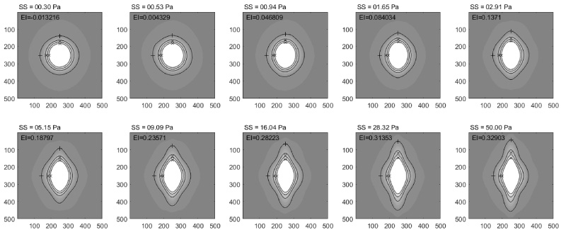
Measured intensity images for 50% rigid cell fraction at various SS ranging from 0.3 Pa to 50 Pa. Intensity levels of the contour plots are 0.15I(0), 0.4I(0), 0.6I(0), and 0.8I(0). The calculated EIs from the intensity level 0.5I(0) are also shown.

Fig. 3.

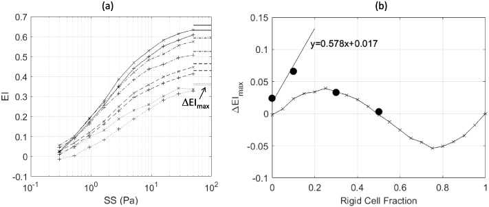
(a) Measured EIs for 0% (solid line), 10% (dash-dot line), 30% (dashed line), and 50% (dotted line) rigid cell fractions at intensity levels 0.15I(0) (+ mark) and 0.8I(0) (× mark). The calculated EI _max values are also shown. (b) Comparison of measured (black circles) and predicted (line with × marks) ΔEI _max values. A line, y = 0.578x + 0.017, representing the data from Rabai et al. [5] is also shown.

Figures 4(a), (b), (c), (d), (e) show the measured intensity images at the SS of 5 PA with RBC counts of 1.20, 1.54, 2.27, 3.29, and 4.16 (10⁶/microliter), respectively. Assuming I _max = 255 for a gray-scale intensity image, corresponding areas are calculated as A = 𝜋ab∕4 in units of pixel² where a is the short axis and b is the long axis of the ellipse at I = 0.8I _max intensity levels. The pixel area vs. number of RBCs is plotted in Fig. 4(f), depicting a nonlinearly increasing area with the increasing RBC count.

Fig. 4.

(a)–(e) Measured intensity images at a SS of 5 PA with RBC counts of 1.20, 1.54, 2.27, 3.29, and 4.16 (10⁶/microliter), respectively. (f) Calculated area of ellipse at I = 0.8Imax intensity levels as a function of RBC counts.

3.2. Estimation of rigid cell fraction and RBC concentration using a CNN

A convolutional neural network was constructed using TensorFlow to estimate poorly deformable cell fraction and RBC concentrations. TensorFlow is an open-source machine learning library that can be utilized in Python and provides packages for deep learning classification problems [9]. The goal of this CNN was to perform sequential label classification for a subset of test images. The same CNN architecture was used for both prediction tasks. This architecture consisted of three convolutional layers with 32, 64, and 128 filters, respectively. These layers contained randomly initialized filters for image feature detection; for example, to detect sharp contrast edges or vertical white lines. Following each convolutional layer was a max pooling layer. The max pooling layer took the maximum value of a particular kernel output. These layers essentially subsampled the input to reduce computational load, memory usage, and number of parameters. This was then fed to two fully connected layers containing 200 neurons and 100 neurons each and finally an output layer with size corresponding to the number of classes in our prediction problem. This architecture is similar to that of the industry standard LeNet-5 architecture, which uses two convolutional layers and three fully connected layers [10]. Exponential Linear Unit (ELU) was used as the activation function for convolutional and hidden layers, while outputs were fed into the softmax function. ELU was used as an activation function as it has been shown to provide optimal accuracy and reduce training time [11]. The softmax function normalizes real output values of the neural network to target class probabilities, ranging from 0 to 1 [12]. This indicates the likelihood of a test sample belonging to a particular class of fraction of rigid cells or concentration of cells. Cross entropy was used as the loss function for training purposes. Training was done using a standard Gradient Descent optimizer with learning rate of .1 and maximum iteration steps of 400. This architecture is summarized in Fig. 5. Training and testing were performed using 20 images per class. Loss as a function of epoch number is plotted in Fig. 6 for both the rigid cell fraction estimation and concentration estimation.

Fig. 5.

The convolutional neural network architecture used for training and softmax classifier prediction.

Fig. 6.

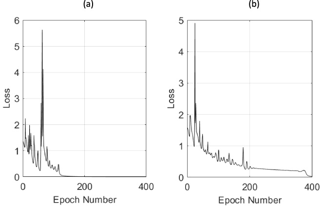
Loss as a function of epoch number for (a) prediction of rigid cell fraction and (b) prediction of the RBC concentration.

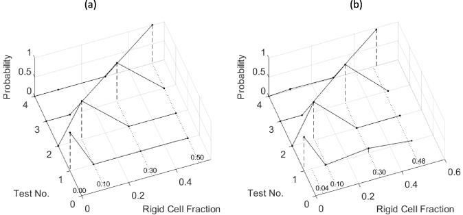
For rigid cell fraction estimation, measured intensity images at a SS of 28.9 Pa are used for training. First, 20 intensity images per class were reduced from 540 × 540 to 60 × 60 pixels by a 2D low-pass filter to decrease computation time during training. Each class represents 0%, 10%, 30%, and 50% rigid cell fractions. Of the 20 images per class, 19 were used for training the CNN, while one image was dropped and subsequently used for testing. Figure 7(a) shows the softmax classification results with assigned probabilities to each class. The discrete probability distribution of each test case represents a probability mass function (PMF) since each class is sequentially labeled as 0%, 10%, 30%, and 50% rigid cell fractions. 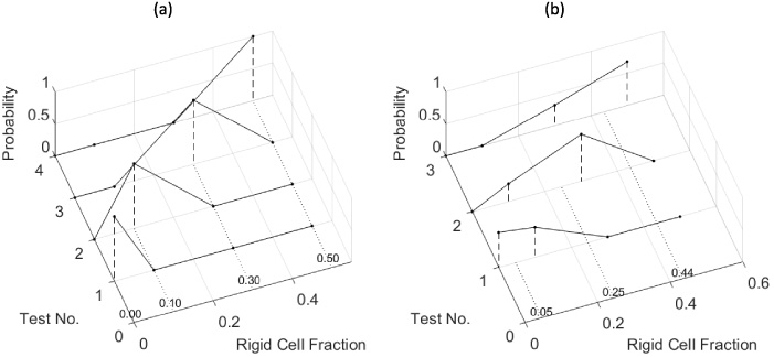Then, the rigid cell fraction for each test case is estimated as the expected value of the discrete random variable: $\begin{eqnarray}\displaystyle E_{n}=\mathop{\sum }_{n_{k}}n_{k}\hat{p}_{k}, & & \displaystyle \nonumber\end{eqnarray}$ where n _k is the rigid-cell fraction and $\hat{p}_{k}$ is the probability estimation of softmax classifier for the kth class. Note that perfect classification of the four classes was obtained. In addition, the prediction capability of the CNN is tested for rigid cell fractions different than those classes used for training. Considering the limited number of classes, three new classes were generated by averaging the images for rigid cell fractions of 0%–10%, 10%–30% and 30%–50%. Figure 7(b) shows the PMF of each class and estimated rigid cell fraction as the expected value of the PMF.

Fig. 7.

Estimation of rigid cell fractions using PMFs from the softmax classifier. (a) Estimated PMFs (dashed vertical lines) of the training classes and expected values (dotted lines) of rigid cell fractions, (b) estimated PMFs (dashed vertical lines) of averaged class images and expected values (dotted lines) of averaged rigid cell fractions.

Similarly, for the RBC concentration estimation, measured intensity images at a SS of 5 Pa are used for training. First, 20 of 100 intensity images per class were reduced from 540 × 540 to 60 × 60 pixels by a 2D low-pass filter to reduce computation time. Each class represents RBC counts of 1.20, 1.54, 2.27, 3.29, and 4.16 (10⁶/microliter). Of the 20 images per class, 19 were used for training the CNN, while one image was dropped and subsequently used for testing. Figure 8(a) shows the PMF of each class and estimated RBC concentration as the expected value of the PMF. Note that perfect classification of the five classes was obtained. In addition, the prediction capability of the CNN is tested for cell concentrations different than those classes used for training. Considering the limited number of classes, four new classes were generated by averaging the images for RBC concentrations of 1.20–1.54, 1.54–2.27, 2.27–3.29, and 3.29–4.16 (10⁶/microliter), Fig. 8(b) shows the PMF of each class and estimated RBC concentration as the expected value of the PMF. These results indicate the robustness of estimation with an increasing order of RBC concentration in between each training class.

Fig. 8.

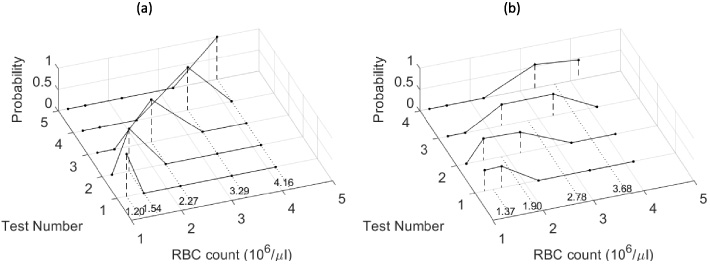
Estimation of RBC concentration using PMFs from the softmax classifier. (a) Estimated PMFs (dashed vertical lines) of the training classes and expected values (dotted lines) of RBC concentration, (b) estimated PMFs (dashed vertical lines) of the averaged class images and expected values (dotted lines) of averaged RBC concentrations.

The robustness of rigid cell fraction estimation by our CNN was also tested using intensity images representing varying RBC concentrations. Synthetic intensity images were generated by multiplying our control intensity data I of four classes of rigid-cell fractions by 0.4 to 1.0 with 0.05 increments. Then, the CNN was trained for four classes of rigid-cell fractions (0%, 10%, 30%, and 50%), with each class having 13 images with differing levels of intensity. The prediction capability of the CNN is tested with intensity images of 0.75I and 0.2I and the results are depicted in Figs 9(a) and 9(b), respectively. Figure 9(a) shows the PMF of each class and estimated rigid cell fraction as the expected value of the PMF using the intensity images of 0.75I. Perfect fractional estimation was obtained for 0.75I since it was in the range of training data. Figure 9(b) shows the PMF of each class and estimated rigid cell fraction as the expected value of the PMF using the intensity images of 0.2I. Although 0.2I was out of the intensity range of training data, fractional estimation was still satisfactory.

Fig. 9.

Estimation of rigid cell fractions using PMFs from the softmax classifier. Each training class has 13 different intensity images ranging from 40% to 100% of the initially measured intensity with 5% increments, simulating various concentrations of an RBC mixture. (a) Estimated PMFs (dashed vertical lines) of the training classes and expected values (dotted lines) of rigid cell fractions using 75% of measured intensity, (b) estimated PMFs (dashed vertical lines) of the averaged classes and expected values (dotted lines) of rigid cell fractions using 20% of measured intensity.

4. Discussion and conclusion

In this paper, we have used an anomalous diffraction model to estimate the light intensity scattered from a mixture of normal and rigid RBCs. The model predicts the same axial ratios as reported by Streekstra et al. for a 1:1 mixture of normal and rigid cells [3]. It was also shown that axial ratio differences between two different intensity levels depend on rigid cell fractions in a complex way. Then, using a LORCA ektacytometer, light intensities were measured at 0%, 10%, 30% and 50% rigid cell fractions at various SS from 0.3 Pa to 50 Pa. It was shown that measured maximum Elongation Index differences (ΔEI _max) are in good agreement with the theoretical predictions. This would imply that a linear relationship between ΔEI _max and sickle cell fractions proposed by Rabai et al. might be valid only for sickle cell fractions less than 0.2 [5].

Then, considering the possible ektacytometer dependency of the deformability measurements and inherent differences between the model predictions and measurements, a Convolutional Neural Network (CNN) is designed to estimate the fraction of rigid RBCs in a mixture using sequentially labeled intensity images for known fractions. Test images within each class provided excellent fraction estimation. Additionally, labeled images were generated by averaging the intensity images using two consecutive classes of rigid cells. These tests also provided excellent results for estimating the increasing order of rigid cell fractions in between each training class.

Similarly, the same algorithm is tested for estimating RBC concentrations from the labeled light intensity images. Test images within each class provided excellent concentration estimation. Additional labeled images were generated by averaging the images of two consecutive classes of RBC concentration. These tests also provided excellent results for estimating the increasing order of RBC concentration in between each training class.

The robustness of rigid cell fraction estimation by our CNN was also tested using intensity images representing differing RBC concentrations. Results showed robust rigid cell fraction estimation even when the CNN was trained with intensity images from varying intra-class RBC concentrations.

It is realized that many pathological samples contain RBCs having a range of mechanical behavior that is not narrowly distributed as in the case of theoretical predictions of mixtures with normal and glutaraldehyde fixed RBCs. A CNN might be a logical choice of estimation method when SC fractions are estimated using pathological samples of RBCs. Similarly, RBC concentration could be readily estimated during a mechanical stability test. In addition, the CNN could be trained for a specific ektacytometer to remove any machine-dependent measurement errors. For example, Rabai et al. [4] reported a constant offset of 10% SC fractions between their global estimation using anomalous diffraction model and true SC fractions. They attributed this offset to spillover of the un-diffracted portion of the laser beam, or possibly from scattering of older, more-rigid cells present in the normal blood. The level of these model/data discrepancies and measurement errors might be different for each ektacytometer. The CNN would be insensitive to these model/data discrepancies and measurement errors since it can be trained for a specific ektacytometer using pathological RBC samples.

Footnotes

Acknowledgements

Experimental part of this work was conducted at Istanbul Koç University School of Medicine, while the first author was a summer researcher. The authors would like to thank the members of the Hemorheology, Hemodynamics and Vascular Biology Laboratory who made this work possible.

References

Mohandas

. Analysis of factors regulating erythrocyte deformability. J Clin Invest. 1980;66:563–73.

Streekstra

Hoekstra

Nijhof

E-J

Heethaar

. Light scattering by red blood cells in ektacytometry: Fraunhofer versus anomalous diffraction. Appl Opt. 1993;32(13):2266. doi:10.1364/ao.32.002266.

Streekstra

Dobbe

JGG

Hoekstra

. Quantification of the fraction poorly deformable red blood cells using ektactyometry. Opt Exp. 2010;18(13):14173. doi:10.1364/oe.18.014173.

Rabai

Meiselman

Wenby

Detterich

Feinberg

. Analysis of light scattering by red blood cells in ektacytometry using global pattern fitting. Biorheology. 2013;49(5–6):317–28. doi:10.3233/bir-2012-0616.

Rabai

Detterich

Wenby

Hernandez

Toth

Meiselman

Deformability analysis of sickle blood using ektacytometry. Biorheology. 2014;51(2–3):159–70. doi:10.3233/bir-140660.

Renoux

Parrow

Faes

Joly

Hardeman

Tisdale

Importance of methodological standardization for the ektacytometric measures of red blood cell deformability in sickle cell anemia. Clin Hemorheol Microcircul. 2016;62(2):173–9. doi:10.3233/ch-151979.

Baskurt

Hardeman

Uyuklu

Ulker

Cengiz

Nemeth

Comparison of three commercially available ektacytometers with different shearing geometries. Biorheology. 2009;46(3):251–64. doi:10.3233/bir-2009-0536.

Baskurt

Meiselman

. Data reduction methods for ektacytometry in clinical hemorheology. Clin Hemorheol Microcircul. 2013;54(1):99–107. doi:10.3233/ch-2012-1616.

Introduction to TensorFlow. TensorFlow. Accessed March 24, 2021. https://www.tensorflow.org/learn.

10.

LeCun

Bottou

Bengio

Haffner

. Gradient-based learning applied to document recognition. Proc IEEE. 1998;86(11):2278–324. doi:10.1109/5.726791.

11.

Clevert

Unterthiner

Hochreiter

, Fast and accurate deep network learning by exponential linear units (ELUs), arXiv:1511.07289, 2015.

12.

Yamashita

Nishio

Kinh Gian Do

Togashi

. Convolutional neural networks: An overview and application in radiology. Insights Imag. 2018;9(4):611–29. doi:10.1007/s13244-018-0639-9.