The study of stresses characteristic of contact mechanism in total knee replacement using two-dimensional finite element analysis

Abstract

The knee joint is one of the more important parts in the human body. Its continuous involvement in the human movement makes it prone to breakage. Due to small contact area, the contact pressure is quite large in this joint. Therefore, the understanding of stresses behavior in knee joint contact is a necessity. In this study, we investigated the stresses behavior in the tibial insert by FEA. A two-dimensional FE model representing the knee joint contact mechanism was created. In the elastic simulation, the contact pressure dropped by 0.2% when the coefficient of friction (CoF) was added. While in the plastic simulation it rose by 12.06%. The average contact pressure fell by 36.42% of the inclusion of plasticity. The CoF lowered the Tresca stress by 0.16% and 12.37% in the elastic and plastic simulation, respectively. Meanwhile, the inclusion of plasticity decreased the average Tresca stress by 74.25%. The CoF, in the elastic simulation, decreased the compressive and tensile stress by 3.29% and 12.46%, respectively. Conversely, in the plastic simulation the compressive stress and tensile rose by 12.01% and 8.20%, respectively. Meanwhile, the inclusion of plasticity caused the compressive stress to decrease by 70.50% and tensile stress to increase by 72.06%.

Keywords

Total knee replacement two-dimensional finite element analysis UHMWPE

1. Introduction

The knee joint is one of the more important parts in the human body. As a voluntary part, its continuous involvement in the human movement makes it prone to breakage [1]. While walking, during the stance phase of the gait cycle, 215% of the body weight is supported by the knee joint at the first peak axial force and 266% at the second peak force [2]. Moreover, 60–80% of the total load is supported by the medial knee compartment. Therefore, the medial compartment is more vulnerable to osteoarthritis than lateral [3].

Unlike the contact mechanism in the hip joint that occurs on an area ranging from 24.7–28.3 cm² [4], the knee joint contact occurs in a small area with an average of 1.4 and 1.8 cm² for the lateral and medial, respectively. And, the contact area will be reduced if the angle of flexion increases [5]. Therefore, the contact pressure is quite large in the knee joint due to smaller contact area and hence results in a large contact pressure. Considering that the knee joint cartilage will be damaged if the impulsive contact stress exceeds 25 MPa [6].

Consequently, the knee joint becomes the most vulnerable joint in the human body. As a comparison, in United State, the overall prevalence of total knee replacement was 4.2% among adults fifty years of age or older [7]. And, because of its vital role in the human mobility, the damage of the knee joint really has hampered the productivity of many its sufferers. So that, at a certain level of damage, the knee joint has to be replaced with an artificial knee joint.

The artificial knee joint installation is expected to last as long as possible, because the damage of the knee joint is not only suffered by old people but also by young people. There are many causes of the knee joint damage. Among others is polyethylene wear. It was reported that according to the revision knee data compiled for 2010 and 2011, 10% of TKR failures were caused by polyethylene wear and 3.2% by periprosthetic fracture [8]. Therefore, the total knee joint replacement patients have to undergo a reoperation for rehabilitation which is not expected by every patient.

To accommodate these failures, we will focus on the failures caused by wear and periprosthetic fracture in the UHMWPE tibial insert. In this study, we will investigate the stresses behavior in the tibial insert by using a two-dimensional finite element analysis (FEA). The stresses that would be investigated are tensile, compressive, and contact pressure. Tresca will also be examined to fully understand the failure of tibial insert.

Fig. 1.

Two two-dimensional cylinders are brought into contact by load P per unit length.

2. Hertzian theory of elastic contact

First of all, we should know that there are some assumptions made in Hertzian theory, namely: the contact surface is continuous and non-conforming, the strains are small, each solid can be considered as an elastic half-space, and the contact surfaces are frictionless [9].

Consider two two-dimensional cylinders with radius $R_{1}$ and $R_{2}$ , modulus of elasticity $E_{1}$ and $E_{2}$ , and Poisson’s ratio $v_{1}$ and $v_{2}$ , respectively, are brought into normal contact by a vertical load P per unit length. The cylinder 1 is on the top and hence the 2 is at the bottom as depicted in Fig. 1. Thus, the half-width of the contact can be calculated by the following equation: $\begin{matrix} (1) & a = \sqrt{\frac{4 P R}{π E^{*}}}, \end{matrix}$ where $E^{*}$ is the equivalent relative modulus of elasticity. R is the equivalent relative radius, it is expressed by $\begin{matrix} (2) & \frac{1}{R} = \frac{1}{R_{1}} + \frac{1}{R_{1}} . \end{matrix}$ And the equivalent relative of modulus of elasticity $E^{*}$ is given by $\begin{matrix} (3) & \frac{1}{E^{*}} = \frac{(1 - v_{1}^{2})}{E_{1}} + \frac{(1 - v_{2}^{2})}{E_{2}} . \end{matrix}$

Meanwhile, the contact pressure along x-axis can be calculated using the following relationship: $\begin{matrix} (4) & p (x) = \frac{2 P}{π a^{2}} \sqrt{(a^{2} - x^{2})} . \end{matrix}$

Its value became zero at the edge of contact ( $x = a$ ), or in the other word, when the value under square root reaches zero. Meanwhile, the maximum contact pressure occurred when the x is zero at the center of contact. The maximum contact pressure ( $p_{0}$ ) can be calculated by using the following equation: $\begin{matrix} (5) & p_{0} = \frac{2 P}{π a} = \sqrt{\frac{P E^{*}}{π R}} . \end{matrix}$

Equations (1), (2), (3), (4), and (5) are used for the contact between two two-dimensional cylinders in z–x plane. For the contact between a cylinder and a plane surface, the above equations also can be used by making $R_{2} = \infty$ . Meanwhile, in the case if one of the parts involved in the contact can be considered as rigid body due to their much difference in the modulus of elasticity between them, we can make use of the equations by making $E = \infty$ for the rigid body. Therefore, for the flat surface of tibial insert, the equivalent relative radius $R = R_{1}$ . And, the femoral component is rigid body, hence the relative modulus of elasticity $E^{*} = E_{2} / (1 - v_{2}^{2})$ . The equations also apply to the contact that occurs between a cylinder and an internal cylinder by taking the R as negative value for internal cylinder [10].

The principal stress in x and z direction in the contact body are given by the following equations [9]: $\begin{array}{l} (6) & σ_{x} = - \frac{p_{0}}{a} {(a^{2} + 2 z^{2}) {(a^{2} + z^{2})}^{- 1 / 2} - 2 z}, \\ (7) & σ_{z} = - a p_{0} {(a^{2} + z^{2})}^{- 1 / 2} . \end{array}$

And the principal shear stress is given by $\begin{matrix} (8) & τ_{1} = \frac{p_{0}}{a} {z - z^{2} {(a^{2} + z^{2})}^{- 1 / 2}} . \end{matrix}$

The maximum principal shear stress ( $τ_{\max}$ ) occurs below the contact surface at the distance of $z_{0} = 0.78 a$ by $0.30 p_{0}$ . As we can see that the entire principal stress in Eqs (6) and (7) are independent of Poisson’s ratio, but for the plane strain, the principal stress in y-direction ( $σ_{y}$ ) should exist and expressed by [9]: $\begin{matrix} (9) & σ_{y} = v (σ_{x} + σ_{z}) . \end{matrix}$

Poisson’s ratio in Eq. (9) depends on the material of the body in which the stresses that would be obtained.

The Hertzian theory of elastic frictionless contact in this study was used for validating the contact simulation that was carried out by using finite element analysis. The validation was conducted to convince us that the model could be used in the entire study. In our case, through the validation, the model would decisively be used in the elastic frictional as well as in the elastic–plastic frictional and frictionless contact mechanism.

3. Finite element (FE) model

3.1. Elastic contact

The simulation would be carried out in a two-dimensional analysis. Hence the two-dimensional model of the total knee replacement was made. There were two parts in this simulation: the femoral circle and the tibial insert. The average size of circle in medial–lateral (frontal) plane of the knee joint has been chosen for representing the femoral circle in this analysis. The medial–lateral (frontal) plane of the knee joint was chosen due to the fact that the stresses are the most sensitive to change in the geometry in this direction as previously reported by Rawlinson and Bartel [11]. Also, it is by this fact that the two-dimensional model in medial–lateral plane can be used to study the behavior of stresses in the total knee replacement that has the complicated shape in the reality.

The radius of femoral circle of 12 mm was taken from the average of medial and lateral condylar half-width of Chinese population as previously reported by Yue et al. [12]. Meanwhile, a rectangular with 96 mm × 48 mm size was made as a representation of tibial insert as the series of forming the model is shown in Fig. 2.

However, in this simulation, the tibial insert was made as an elastic half-space. Therefore, the size of tibial insert was set to have the length of eight times femoral circle radius and four times for the thickness. The model is clearly shown in Fig. 3.

To allow the local seeding, mesh flow, and density of element, the tibial insert body was partitioned into five segments as shown in Fig. 3. Among the segments, the rectangle at the upper middle of tibial insert is the most important segment due to its direct contact with the femoral circle, and also it is an area of interest in this work at which the subsurface stresses and contact pressure to be observed. This segment would be finely meshed. Its edges were locally meshed with the approximate element size of 0.1 mm.

Fig. 2.

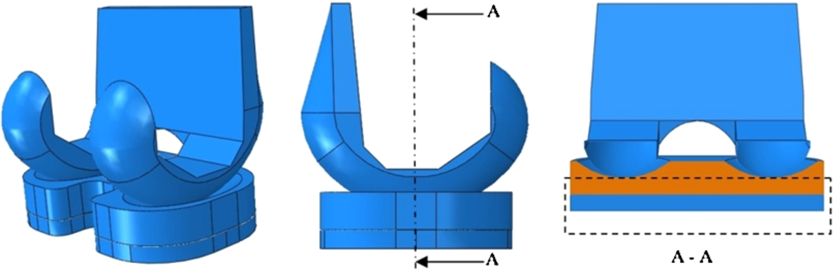
The total knee replacement (TKR) (left). Its side view with line to indicate cut view path (middle). Cut view of TKR (right), the dashed rectangle is the tibial insert representation in this simulation.

Fig. 3.

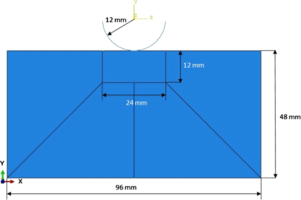
The two-dimensional contact model with the partition measurements.

Fig. 4.

The elastic half-space of two-dimensional FE model of tibial insert.

Meanwhile, the edges those surround the rectangular segment was controlled by number local seeding method with 33 numbers of element and 5 bias ratio. The rest of edges with no direct connection with the rectangular segment were automatically seeded by the ABAQUS software. In this simulation we assumed that the model as a plain strain. Therefore, a four-node bilinear plane strain quadrilateral (CPE4) was chosen as the element type, as we can see in Fig. 4.

The tibial insert was modeled as a deformable body with UHMWPE as its material. Meanwhile, the femoral circle was modeled as a rigid body for its much higher modulus of elasticity compared with UHMWPE. The modulus of elasticity of UHMWPE was extracted from the nonlinear true stress-true strain curve that previously used by Halloran et al. [13] as depicted in Fig. 5.

The modulus of elasticity was obtained by dividing the first nonzero true stress by the first nonzero true strain. From Fig. 5, we got that the first nonzero true stress is 11 MPa and the corresponding true strain is 0.02, then it yields the modulus of elasticity of 550 MPa. A Poisson’s ratio of 0.44 was used to be consistent with the previous simulation done by Willing and Kim [14].

Fig. 5.

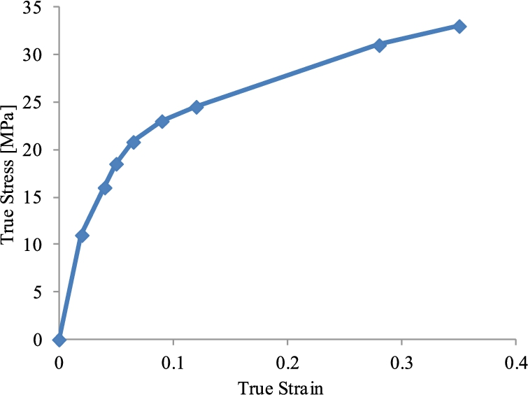
Nonlinear true stress-true strain of UHMWPE [13].

The frictionless surface-to-surface with hard contact relationship was chosen for the contact interaction. The outer surface of femoral circle was chosen as the master surface, while the upper edge of rectangular partition of the tibial insert was chosen as the slave surface. The load per unit length of 300 N/mm was applied to the femoral circle reference point. This load is the in vivo knee joint load of 2000 N with contact width of 6–7 mm as it had been used by Rawlinson and Bartel [11] in the previous report. The tibial insert was fixed in all direction at the bottom surface to avoid from any translations and rotations. Meanwhile the femoral circle was allowed to translate in y direction and fixed in the rest degree of freedom.

3.2. Elastic–plastic contact

In the elastic–plastic contact, there were some additional data should be entered in the simulation, such as true stress versus plastic strain. The plastic strain $ε_{pl}$ was obtained by extracting the data from the nonlinear true stress-true strain of UHMWPE curve in Fig. 5 using the following formula: $\begin{matrix} (10) & ε_{pl} = ε_{true} - \frac{σ_{true}}{E}, \end{matrix}$ where $ε_{true}$ is the true strain, $σ_{true}$ is the true stress, and E is modulus of elasticity. Here, the true stresses are the yield stresses with correspond plastic strain as the effect of the strain hardening. The yield stress versus plastic strain as an input data into ABAQUS material property are tabulated in Table 1. The coefficient of friction was adopted from the work of Godest et al. [15] in which they applied the coefficient of friction of 0.04. The other parameters such as load, the mesh density, and the element type were the same as in the elastic contact simulation.

Table 1
Yield stress versus plastic strain of UHMWPE as the input for Abaqus material property

Yield stress [MPa] Plastic strain

11 0.00

16 0.01

18.5 0.02

20.8 0.03

23 0.05

24.5 0.08

31 0.22

33 0.29

Yield stress [MPa]	Plastic strain
11	0.00
16	0.01
18.5	0.02
20.8	0.03
23	0.05
24.5	0.08
31	0.22
33	0.29

To determine the influence of the coefficient of friction on the elastic and plastic simulation, we conducted four types of simulations: elastic with (elastic frictional) and without friction (elastic frictionless), and plastic with (plastic frictional) and without friction (plastic frictionless). With these four types of simulation, we could know not only the characteristics of the elastic and plastic contact, but also can determine the effect of the coefficients of friction on both simulations.

4. Results and discussion

4.1. Elastic contact

The contact parameters attained by Hertzian theory as well as FEA were summarized in the Table 2. If we refer to the work of van den Heever et.al [16] and Rawlinson and Bartel [11], in which they took 5% as the limit of error, the absolute maximum shear stress and its position below the counterface seem to be out of the limit. The FEA underpredicted the depth of maximum absolute shear stress by 12.74%. On the contrary, the value of absolute maximum shear stress was overpredicted by 7.02%. However, the good news came from the contact half-width and maximum contact pressure. They differed with Hertzian contact by only 3.38% and 0.39%, respectively. This validation error is smaller than that was reported by Simpson et al. in which they got the error by 14% and 21% for contact pressure and half-width, respectively [17].

Table 2
The result of contact parameters using Hertzian theory and FEA

Parameters Descriptions Hertzian FEA Unit

a Half width 2.59 2.68 mm

$p_{0}$ Maximum contact pressure 73.67 73.96 MPa

$z_{0}$ The depth of maximum shear stress 2.04 1.78 mm

$τ_{\max}$ Absolute maximum shear stress 22.10 23.88 MPa

Parameters	Descriptions	Hertzian	FEA	Unit
a	Half width	2.59	2.68	mm
$p_{0}$	Maximum contact pressure	73.67	73.96	MPa
$z_{0}$	The depth of maximum shear stress	2.04	1.78	mm
$τ_{\max}$	Absolute maximum shear stress	22.10	23.88	MPa

The principal stress in x, y, and z direction, the principal shear stress, and the maximum absolute shear stress, which obtained by Eqs (6), (7), (8), and (9), were depicted in Fig. 6. The absolute shear stress $τ_{\max}$ along z-axis below the counterface were obtained by the following conditions: For $0 ⩽ z ⩽ 0.3$ , $τ_{\max} = (σ_{y} - σ_{z}) / 2$ . For $z ⩾ 0.3$ , $τ_{\max} = (σ_{x} - σ_{z}) / 2$ .

The comparison between the Hertzian and FEA of absolute shear stress is shown in the Fig. 7. The FEA overpredicted the absolute shear stress by average of 11.74%. The highest deviation was occurred at the counterface and continued to decline along the z-axis below the counterface. The absolute maximum shear stress took place at 1.78 mm below the counterface. Meanwhile, in Hertzian, the maximum absolute shear stress occurred at 2.04 mm below the counterface by 22.10 MPa as tabulated in Table 2.

Fig. 6.

The stresses–distance below the counterface curve obtained by Hertzian theory.

Fig. 7.

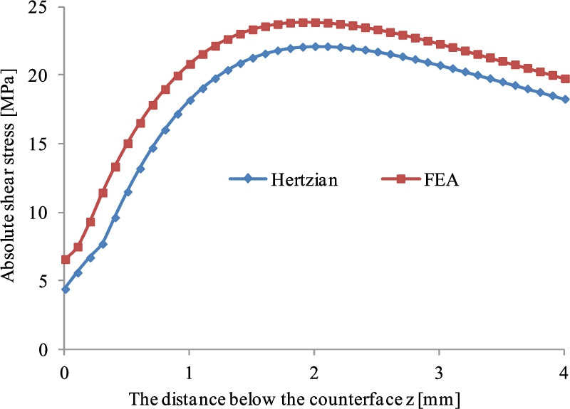
The absolute shear stress obtained by both Hertzian elastic contact and FEA along z-axis below the counterface.

A good agreement between FEA and Hertzian was observed in contact pressure as can be seen in Fig. 8. Unlike in z-direction, the change of the element size along x-axis from the contact center was insignificant. Thus, the curve intended for comparing Hertzian and FEA contact pressure could be easily drawn as shown in Fig. 8. There was an interesting case as a result of the Hertzian and FEA contact half-width difference value of 2.58 mm and 2.68, respectively. Due to the half width difference, the zero contact pressure would begin at a different point. Therefore, FEA contact pressure curve would deviate from Hertzian after 2.58 mm. And, the FEA contact pressure curve would reach zero value at 2.68 mm. As a result of this phenomenon, we could take 85% of half-width as a distance limit from contact center for a good agreement result between Hertzian and FEA. However, in general, the result of FEA was representative enough of Hertzian theory. Therefore, the model can be used for further simulation, namely for the elastic frictional and the elastic–plastic frictional and frictionless contact simulation.

Fig. 8.

The contact pressure along the positive x-axis from the center obtained by both Hertzian theory and FEA.

4.2. Elastic–plastic contact

When the elastic simulation involved the coefficient of friction, the maximum contact pressure was slightly increased by 0.52%, from 73.96 MPa to 74.34 MPa. Meanwhile, in the plastic simulation, it only resulted in a slight rise by 0.06%, from 47.13 MPa to 47.14 MPa. Figure 9 shows that it was clearly visible that the inclusion of plasticity of UHMWPE highly affected the contact pressure. The average of maximum contact pressure in the elastic simulation was 74.15 MPa and it dropped to 47.14 MPa after the inclusion of plasticity. The contact pressure drop reached 36.42% which was fairly large.

Meanwhile, the maximum Tresca stress showed a different trend as shown in Fig. 10. The Tresca stress decreased when the coefficient of friction was involved in the elastic as well as plastic simulation. For the elastic simulation, the maximum Tresca stress decreased by 0.16% from 47.75 MPa to 47.67 MPa after the inclusion of the coefficient of friction. The same trend also occurred in the plastic simulation. The coefficient of friction lowered the maximum Tresca stress by 12.37% from 27.43 MPa to 27.33 MPa. As noted previously, the increasing or the decreasing of the stresses was greatly affected by the plasticity of the UHMWPE. Thus we can see that the maximum Tresca stress was observed to drop by 74.25% from 47.71 MPa to 27.38 MPa.

We chose the Tresca stress in our study due to the fact that the safety area of Tresca stress curve is smaller than that of von Mises stress area. It means that the Tresca failure criterion is safer than that of von Mises stress. As we know that our study involved the human body (knee joint), we preferred the Tresca stress than von Mises stress.

Fig. 9.

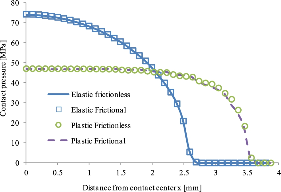
Contact pressures obtained by FEA for elastic and plastic simulation. Each simulation was conducted with and without friction.

Fig. 10.

Tresca stress below the surface of contact for all contact mechanism.

Fig. 11.

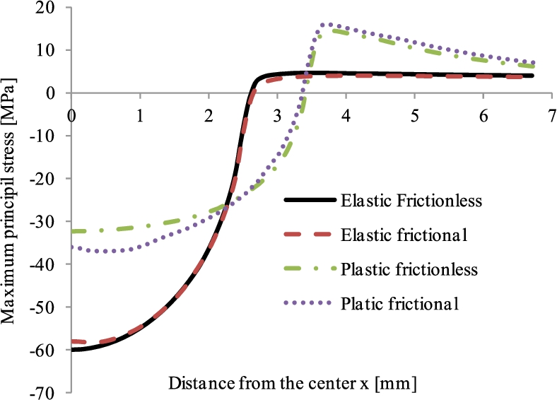
Maximum Principal stress along x-axis from the center of contact point.

In this simulation, we also monitored the compressive and tensile stress at the counterface. Figure 11 shows that the compressive stress occurred at the counterface area involved. While on the outside of the contact area, the compressive stress was turned into tensile stress. The farther from the contact center, the compressive stress is getting smaller and eventually turned into the tensile stress immediately after passing the contact area.

For the elastic frictionless contact simulation, the maximum compressive stress of 60.03 MPa occurred right at the contact center. Then, its value gradually changed into the tensile stress that reached the maximum value of 4.47 MPa at 3.49 mm from the contact center. Meanwhile, when coefficient of friction was included in the simulation, the maximum compressive stress decreased by 3.29% to 58.12 MPa. But, this time, the maximum compressive stress did not take place at the contact center as in the elastic frictionless simulation. It, however, moved to a distance of 0.30 mm from the contact center. Meanwhile, the maximum tensile stress took place at a distance of 4.10 mm by 3.98 MPa. It decreased by 12.46%.

In the plastic simulation, we can see that the maximum compressive stress of 32.43 MPa also occurred at the contact center if we simulated without friction. The position was similar to that occurred in the elastic simulation. And, the maximum tensile stress of 14.47 MPa took place at 3.69 mm from the contact center. Meanwhile, when friction was included in the simulation, the maximum compressive stress increased by 12.01% to be 36.86 MPa, which occurred at 0.49 mm. And, the maximum tensile stress also increased by 8.20% to be 15.76 MPa. The inclusion of plasticity resulted in the compressive stress to decrease by 70.50% and tensile stress to increase by 72.06% inversely.

Based on the result aforementioned; we know that the inclusion of the coefficient of friction gave a different effect on elastic and plastic simulation. In the elastic one, the coefficient of friction resulted in the increasing of the maximum tensile and compressive stress. In contrast to the plastic simulation, the maximum tensile and compressive stress decreased by the inclusion of friction coefficient. And there was one unique phenomenon took place when coefficient of friction was included, namely the maximum compressive stress did not happen at the contact center, but shifted away from the contact center. The summary of all phenomena can be seen in Fig. 12.

Fig. 12.

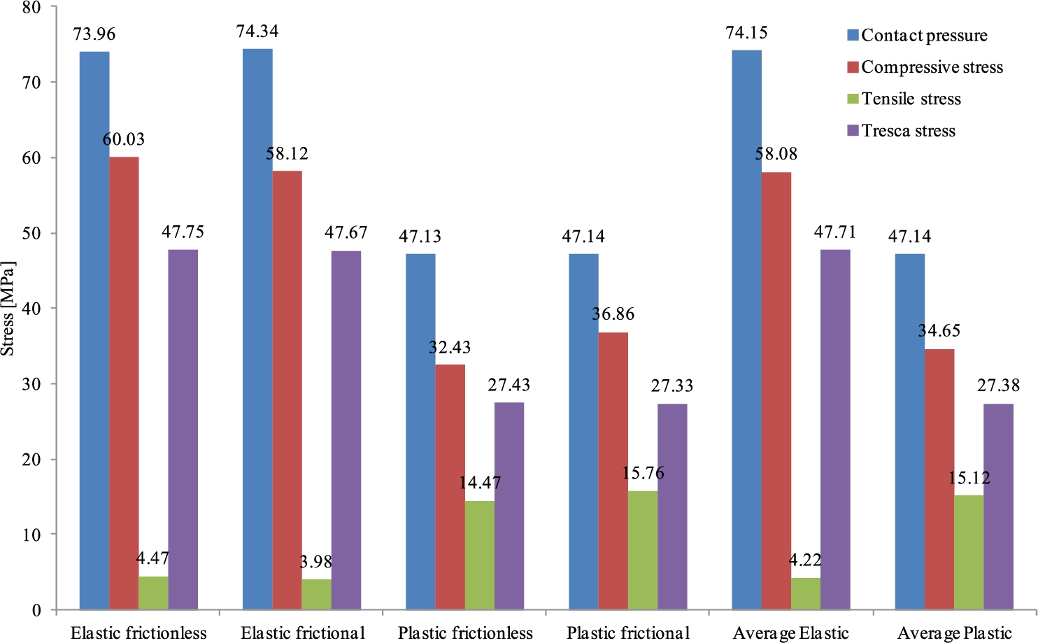
Summary of simulations.

5. Conclusions

In the elastic simulation, the contact pressure dropped by 0,2% when the coefficient of friction was added. While in the plastic simulation it only raised the contact pressure by 12.06%. The average contact pressure fell by 36.42% due to the inclusion of plasticity.

The coefficient of friction lowered the Tresca stress by 0.16% and 12.37% in the elastic and plastic simulation, respectively. Meanwhile, the inclusion plasticity resulted in the average Tresca stress dropped by 74.25%.

The coefficient of friction, in the elastic simulation, caused the compressive and tensile stress to decrease by 3.29% and 12.46%, respectively. Conversely, in the plastic simulation the compressive stress and tensile rose by 12.01% and 8.20%, respectively. Meanwhile, the inclusion of plasticity resulted in the compressive stress to decrease by 70.50% and tensile stress to increase by 72.06% inversely.

Conflict of interest

The authors have no conflict of interest to report.

References

Shah

Bhave

and Sonetha

, Fatigue analysis of the knee joint, in: International Conference on Advanced Computing Technologies and Applications (ICACTA), Mumbai Vasudevan

Joshi

A.R.

and Shekokar

N.M.

, eds, Elsevier, 2015, pp. 250–255.

Halder

Kutzner

Graichen

Heinlein

Beier

and Bergmann

, Influence of limb alignment on mediolateral loading in total knee replacement: In vivo measurements in five patients, Journal of Bone & Joint Surgery 94(11) (2012), 1023–1029.

Schwachmeyer

Kutzner

Bornschein

Bender

Dymke

and Bergmann

, Medial and lateral foot loading and its effect on knee joint loading, Clinical Biomechanics 30(8) (2015), 860–866. doi:10.1016/j.clinbiomech.2015.06.002.

Palastanga

Field

and Soames

R.W.

, Anatomy and Human Movement, 2nd edn, Elsevier, 1994.

Walker

P.S.

and Hajek

J.V.

, The load-bearing area in the knee joint, Journal of Biomechanics 5(6) (1972), 581–584. doi:10.1016/0021-9290(72)90030-9.

Heijink

Gomoll

A.H.

Madry

Drobnič

Filardo

Espregueira-Mendes

et al., Biomechanical considerations in the pathogenesis of osteoarthritis of the knee, Knee Surgery, Sports Traumatology, Arthroscopy 20(3) (2012), 423–435. doi:10.1007/s00167-011-1818-0.

Weinstein

A.M.

Rome

B.N.

Reichmann

W.M.

Collins

J.E.

Burbine

S.A.

Thornhill

T.S.

et al., Estimating the burden of total knee replacement in the United States, Journal of Bone & Joint Surgery 95(5) (2013), 385–392. doi:10.2106/JBJS.L.00206.

Schroer

W.C.

Berend

K.R.

Lombardi

A.V.

Barnes

Bolognesi

M.P.

Berend

M.E.

et al., Why are total knees failing today? Etiology of total knee revision in 2010 and 2011, Journal of Arthroplasty 28(8) (2013), 116–119. doi:10.1016/j.arth.2013.04.056.

Johson

K.L.

, Contact Mechanics, Cambridge University Press, Cambridge, 1985.

10.

Budynas

R.G.

and Nisbett

J.K.

, Shigley’s Mechanical Engineering Design, 9th edn Lange

, ed., McGraw-Hill, New York, 2011.

11.

Rawlinson

J.J.

and Bartel

D.L.

, Flat medial–lateral conformity in total knee replacements does not minimize contact stresses, Journal of Biomechanics 35(1) (2002), 27–34. doi:10.1016/S0021-9290(01)00172-5.

12.

Yue

Varadarajan

K.M.

Tang

and Rubash

H.E.

, Gender differences in the knees of Chinese population, Knee Surgery, Sports Traumatology, Arthroscopy 19(1) (2011), 80–88.

13.

Halloran

J.P.

Petrella

A.J.

and Rullkoetter

P.J.

, Explicit finite element modeling of total knee replacement mechanics, Journal of Biomechanics 38(2) (2005), 323–331. doi:10.1016/j.jbiomech.2004.02.046.

14.

Willing

and Kim

I.Y.

, Three dimensional shape optimization of total knee replacements for reduced wear, Structural and Multidisciplinary Optimization 38(4) (2009), 105–414. doi:10.1007/s00158-008-0281-0.

15.

Godest

A.C.

Beaugonin

Haug

and Taylor

, Simulation of a knee joint replacement during a gait cycle using explicit finite element analysis, Journal of Biomechanics 35(2) (2002), 267–275. doi:10.1016/S0021-9290(01)00179-8.

16.

van den Heever

D.J.

Scheffer

Erasmus

and Dillon

, Contact stresses in a patient-specific unicompartmental knee replacement, Clinical Biomechanics 26(2) (2011), 159–166. doi:10.1016/j.clinbiomech.2010.09.007.

17.

Simpson

D.J.

Gray

D’Lima

Murray

D.W.

and Gill

H.S.

, The effect of bearing congruency, thickness and alignment on the stresses in unicompartmental knee replacements, Clinical Biomechanics 23(9) (2008), 1148–1157.