New evaluation indices for rotational knee angles in standing anteroposterior knee radiographs

1. Introduction

Knee osteoarthritis (OA) is associated with the change of lower extremity alignment in longitudinal epidemiological studies [1–3]. Advanced knee OA demonstrated three-dimensional (3D) structural and alignment changes in not only a coronal plane but also sagittal and axial planes (e.g., external rotation of the femur relative to the tibia and decreased femoral neck anteversion) [4–6].

The most suitable method of evaluating the image findings in elucidating the etiology of knee OA is the longitudinal study [1–3,7,8]. Our group has been conducting an epidemiological study on knee OA in the Matsudai district of Tokamachi City, Niigata Prefecture, in 7-year intervals since 1979 (Matsudai Knee Osteoarthritis Survey: MKOS) [7–15]. Although this study has acquired X-ray images in the coronal and sagittal planes, it has not been able to assess rotational knee alignment. Identifying the time course of rotational knee alignment is crucial for the pathophysiology of knee OA [4,5,7,16,17].

The evaluation of rotational knee alignment between the femur and tibia is generally performed in a 3D space using computed tomography (CT) and magnetic resonance imaging (MRI). However, CT and MRI are difficult to apply to many cases in longitudinal studies, such as MKOS. Although an accurate assessment of rotational knee angles is impossible in 2D radiographs [4,16–22], the approximated time course for rotational knee alignment is desired to be determined from anteroposterior (AP) radiographs for the same subjects.

As anteroposterior (AP) radiographs were taken under standing conditions in MKOS [7–15], the simulation study to calculate the estimated rotational knee angles would have been more preferable in the standing position than the supine. However, since common image modalities, such as CT and MRI, are performed on subjects in the supine position, the simulation study is difficult to conduct on subjects in the standing position when using these modalities. In our group, the 3D lower extremity alignment assessment system (Knee CAS^®, LEXI, Inc., Tokyo, Japan), which can evaluate the standing position with high accuracy, was developed [4,6,16,17,23–33]. This system used 3D-to-2D image registration techniques based on biplanar long lower extremity radiographs.

The aim of this study was to (1) identify the relationship between changes in rotational indices and the simulated rotational knee angles in the standing position, (2) propose a regression equation for calculating the changes in relative rotational angles between the femur and tibia in standing AP radiographs, and (3) to verify the accuracy of the proposed regression equation.

2. Methods

2.3. Rotational indices in standing anteroposterior radiographs

The rotational indices determined from the standing AP radiographs in MKOS were as follows (Fig. 1): (1) the rotational index of the femur (defined by the distance denoted by “P” between the sphere center of the medial posterior femoral condyle and the lateral edge of the patella) and (2) the rotational index of the tibia (defined by the distance denoted by “F” between the medial eminence of the tibia and the lateral edge of the fibula head). The “P” and “F” indices were standardized by the diameter of the sphere of the medial posterior femoral condyle, denoted by “M”, resulting in the derivation of the standardized rotational indices P/M and F/M. Regarding the reliability of the rotational indices, the intra-observer reproducibility, through an intra-class correlation coefficient (ICC) (1, 1), was 0.98, 0.99, and 0.98 for indices “M”, “P”, and “F”, respectively. The inter-observer reproducibility, through an inter-class correlation coefficient (ICC) (2, 1), was 0.98, 0.98, and 0.98 for indices “M”, “P”, and “F”, respectively [35].

OPEN IN VIEWER

Fig. 1.

Rotational indices. The femoral rotational index is the distance between the sphere center of the medial posterior femoral condyle and the lateral edge of the patella. The tibial rotational index is the distance between the medial eminence of the tibia and the lateral edge of the fibula head. They are standardized by the diameter of the sphere of the medial posterior femoral condyle.

2.4. 3D bone model and coordinate system

Digital 3D models of the femur and tibia were reconstructed from CT data (SOMATOM Sensation 16, Siemens Inc., Munich, Germany) using 3D visualization and modeling software (ZedView^®, LEXI Inc., Tokyo, Japan). The anatomical coordinate system was established according to the definition provided by Sato et al. [23] (Fig. 2). The femoral x-axis was defined as the line connecting the centers of the medial and lateral posterior femoral condyle spheres (laterally positive). The femoral y-axis was defined as a line perpendicular to the plane connecting the centers of the femoral head and approximated medial and lateral posterior condyle spheres (anteriorly positive). The femoral z-axis was defined as the cross product of the x- and y-axes (superiorly positive). The tibial z-axis was defined as the line connecting the midpoint of the tibial eminences and those of the medial and lateral tops of the talar dome (superiorly positive). The tibial y-axis (anteriorly positive) was defined as the line connecting the z-axis with the point of the tibial insertion at the posterior cruciate ligament. The tibial x-axis was defined as the cross product of the z- and y-axes (laterally positive). To detect the position of the femur, tibia, and patella in relation to the ground, the world coordinate system with the photography platform was constructed.

OPEN IN VIEWER

Fig. 2.

Anatomical coordinate system defined on (a) the femur and (b) the tibia. The femoral x-axis was defined as the line connecting the centers of the medial and lateral posterior femoral condyle spheres (laterally positive). The femoral y-axis was defined as a line perpendicular to the plane connecting the centers of the femoral head and approximated medial and lateral posterior condyle spheres (anteriorly positive). The femoral z-axis was defined as the cross product of the x- and y-axes (superiorly positive). The tibial z-axis was defined as the line connecting the midpoint of the tibial eminences and those of the medial and lateral tops of the talar dome (superiorly positive). The tibial y-axis (anteriorly positive) was defined as the line connecting the z-axis with the point of the tibial insertion at the posterior cruciate ligament. The tibial x-axis was defined as the cross product of the z- and y-axes (laterally positive).

2.5. Simulation study of knee rotation

The positions of the femur, tibia, and patella under standing conditions in the world coordinate system were determined using the semi-automatic 3D–2D image registration technique, which involved matching 3D bone models with biplanar radiographs under standing conditions [4,6,16,17,23–33] (Fig. 3). To investigate the relationship between the rotational indices (P/M and F/M) and simulated rotational knee angles, 3D bone models were rotated around the femoral z-axis from an internal rotation angle of 10° to an external rotation angle of 10° at every 2.5° (Fig. 4). To obtain the DRR images, the raw CT data were incorporated into each 3D bone model at each simulated rotational angle using the 3D-3D image registration technique (Fig. 5); thus, DRR images of the 3D bone models at every 2.5° of rotation were acquired. The correlation between the simulated rotational knee angles and the rotational indices (P/M and F/M) in DRR images was evaluated.

OPEN IN VIEWER

Fig. 3.

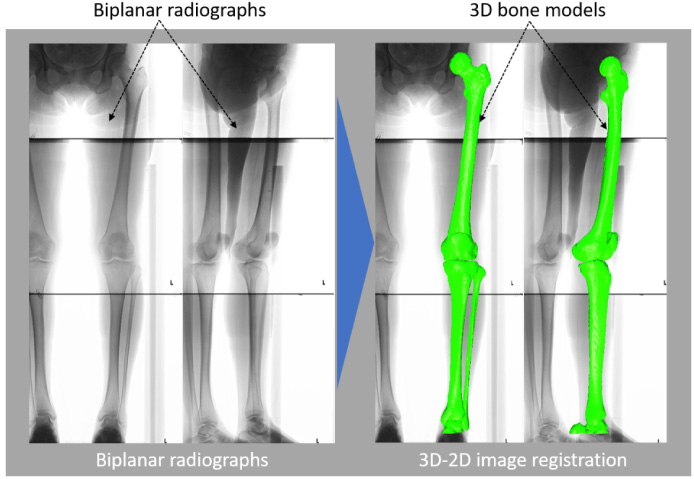
Three-dimensional to two-dimensional (3D–2D) image registration technique in biplanar long-leg radiographs under the standing positions. To obtain standing positions, 3D bone models and biplanar radiographs were matched by the semi-automatic 3D–2D image registration technique.

OPEN IN VIEWER

Fig. 4.

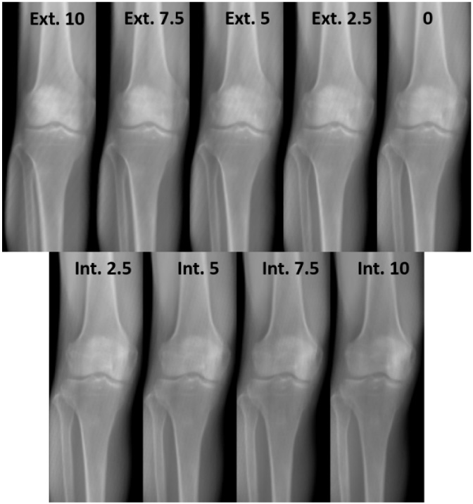
Simulation of knee rotation. Three-dimensional bone models were rotated around the femoral z-axis from an internal rotation of 10° to an external rotation of 10° at every 2.5°.

OPEN IN VIEWER

Fig. 5.

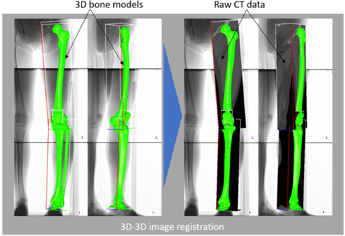
Three-dimensional to 3D (3D-3D) registration technique between 3D bone models and raw CT data. To obtain digitally reconstructed radiography (DRR) images, raw CT data was incorporated into each 3D bone model at each simulated rotational angle, respectively, using the 3D-3D image registration technique; thus, the DRR images of 3D bone models at every 2.5° of rotation were acquired.

2.7. Verification of accuracy of regression equation

The lower limb of a healthy elderly female volunteer from the participants was examined. Firstly, for two models, the femur underwent internal and external rotation of 2.5° around the femoral z-axis, based on the tibia. DRR images in the three-orthogonal direction (front, inside, and outside) were acquired (Fig. 6), and the rotational indices in DRR images were measured. Secondly, the change in relative rotational angles between the femur and tibia were calculated using the derived regression equation. Finally, the errors of the calculated changes in relative rotational angles between the femur and tibia relative to the exact value (internal and external rotation of 2.5°) were evaluated.

OPEN IN VIEWER

Fig. 6.

Verification of accuracy of regression equation (a) external rotation and (b) internal rotation of femur based on tibia. Two models were obtained, in which the femur was rotated around the femoral z-axis based on the tibia with internal and external rotations of 2.5°, and three-direction DRR images (front, inside, and outside) were acquired.

3. Results

The index “M” maintained an almost constant rotational angle value ranging from −10 (internal) to 10 (external) degrees in each of the male and female groups, and its mean ± SD values were 41.7 ± 0.2 mm and 45.2 ± 0.3 mm in females and males, respectively (Fig. 7). This result suggested that the index “M” could be the optimal parameter to be adopted as the standard value.

OPEN IN VIEWER

Fig. 7.

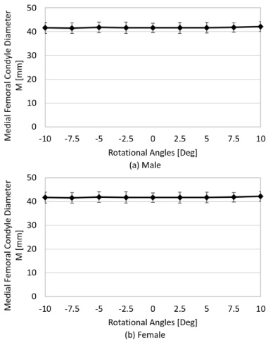
Index “M” is shown at each rotational angle of every 2.5° from an internal rotation of 10° to an external rotation of 10° in a knee joint. The index “M” maintained an almost constant rotational angle value ranging from −10 (internal) to 10 (external) degrees in each of the male and female groups, and its mean ± SD values were 41.7 ± 0.2 mm and 45.2 ± 0.3 mm in females and males, respectively.

In the simulation study, the standardized femoral rotational index “P/M” linearly increased in direct proportion to the simulated rotational knee angle (male: r = 0.99, p < 0.0001; female: r = 0.98, p < 0.0001) (Fig. 8). The standardized tibial rotational index “F/M” linearly decreased with an increase in the simulated rotational knee angle (male: r = 0.99, p < 0.0001; female: r = 0.98, p < 0.0001) (Fig. 9).

OPEN IN VIEWER

Fig. 8.

Correlation between the standardized femoral rotational index “P/M” and the simulated rotational knee angle. In the simulation study, the standardized femoral rotational index “P/M” linearly increased in direct proportion to the simulated rotational knee angle (male: r = 0.99, p < 0.0001; female: r = 0.98, p < 0.0001).

OPEN IN VIEWER

Fig. 9.

Correlation between the standardized tibial rotational index “F/M” and the simulated rotational knee angle. The standardized tibial rotational index “F/M” linearly decreased with an increase in the simulated rotational knee angle (male: r = 0.99, p < 0.0001; female: r = 0.98, p < 0.0001).

The relationships between the simulated rotational knee angles and the standardized rotational indices (P/M and F/M) had to be mathematically formulated. As the relationships between the simulated rotational knee angles and the standardized rotational indices (P/M and F/M) were linear as mentioned above (Figs 8 and 9), their regression equations were formulated as follows:

The regression equations for femur and tibia were expressed as linear functions (1) and (2), respectively, in the following manner: (1) (2) where y _f and y _t are the standardized rotational index values of femur (P/M) and tibia (F/M), respectively; x is the simulated rotational knee angle; a is the slope; b is the intercept of the standardized rotational index with the simulated rotational knee angle; and the subscripts f and t represent femur and tibia, respectively.

From Eqs (1) and (2), the relative rotational angles between the femur and tibia before and after rotation, namely 𝛿₁ and 𝛿₂, respectively, were obtained as follows: (3) (4) where the subscripts 1 and 2 mean represent the pre-positional and post-rotational positions, respectively.

From Eqs (3) and (4), the chronological change in the relative rotational angle between the femur and tibia (𝛿) was eventually obtained as follows: (5) Substituting the precisely identified numerical values into Eq. (5), 𝛿 for the male and female groups was conclusively obtained as follows:

For males, (6) and for females, (7) Where the subscripts m and f represent male and female, respectively.

To verily the accuracy of regression Eqs (6) and (7), the errors of the calculated changes in relative rotational angles between the femur and tibia relative to the exact value (internal and external rotation of 2.5°) were evaluated (Fig. 6). The resulting error was 0.45 ± 0.26° (mean ± SD), and the maximum error was 0.80°.

As the unique features of this study are summarized, the use of DRR images in the simulation study must be discussed first. The DRR images were projections of 3D bone models on the 2D plane (Fig. 5), such that rotational movement was accurately reflected in the changes in rotational indices. Secondly, the DRR images were constructed in the “standing position” to adjust to the standing AP radiographs in MKOS [7–15]. Common modalities, such as CT and MRI alone, cannot assess subjects in the standing positions. However, 3D–2D image registration techniques [4,6,16,17,23–33] (Fig. 3) can provide standing DRR images. Thirdly, the selection of rotational indices, especially using of the medial posterior femoral condyle as the standardized index, could provide high reproducibility because this condyle can be approximated as the “sphere” [4,6,16,17,23–33] (Fig. 1); therefore, its diameter is hardly affected by knee rotation within the narrow range (Fig. 6).

This study was limited by the fact that the regression equations were formulated using data from a limited number of subjects. In addition, the application of these equations to other subjects may not necessarily produce optimal results. Notwithstanding, the equations can potentially determine the “probable change in rotational knee angles” for the “same subjects” in MKOS.

Each of the “M”, “P”, and “F” indices was found to be considerably stable in this study (Fig. 1). The index “M” yielded an absolutely small standard deviation relative to its mean value, such that we decided to utilize the index “M” as the standardized parameter. The medial posterior femoral condyle can be approximated as the “sphere” [4,6,16,17,23–33]. It was realized that the diameter of the “sphere” was hardly affected by knee rotation within the narrow range, namely the range from internal rotation of 10° to external rotation of 10° (Fig. 6). The femoral rotational index “P” was the suitable parameter because its definition entailed using the center point uniquely determined in the medial posterior femoral condyle “sphere”. As for the tibial rotational index “F”, the medial eminence of the tibia and the lateral edge of the fibula were easily detected, and these features resulted in the high ICC [35]. In addition, the close position of the medial eminence of the tibia to the center of the knee joint as well as the most lateral location of the lateral edge of the fibula from the center of knee joint made “F/M” the suitable index for better predicting of the simulated rotational knee angle.

OPEN IN VIEWER

Fig. 10.

Cosine function and linear approximations of 𝜃 _f and 𝜃 _t in the range of ±10°. In the rotation between the femur and tibia, there is almost no possibility that the internal and external rotations exceed the range of ±10°. Therefore, it was verified if the ranges of 50° <  𝜃 _f < 70° and 20° <  𝜃 _t < 40° could be approximated with a linear function at the rotational indices of rotation changes.

The reasons behind the directly proportional linear increment of the standardized femoral rotational index “P/M” with the simulated rotational knee angle were as follows: firstly, the DRR images, which were constructed by projecting the 3D bone models on the coronal plane, were applied, that is, the DRR images were the 3D bone models themselves (Fig. 5); secondly, the semi-automatic 3D–2D image matching technique with high accuracy [24] enabled the DRR images (2D projection images) to precisely reproduce rotational knee alignment in the “standing position” (Fig. 3). To adjust to the standing AP radiographs in MKOS, the simulation study should have reproduced the “standing position”. In our group, contours of the femur and tibia in biplanar radiographs were detected according to the method described by Canny [36]. Projected outline points of each 3D model were the finite edge points of the 2D shadow produced from the projections of all visible triangular surfaces of the 3D model [24]. Subsequently, this 3D–2D image registration technique enabled 3D digital bone models to be projected onto biplanar radiographs [4,6,16,17,23–33]. The accuracy of the 3D–2D image registration technique was established as follows: three spherical markers were attached to each sawbone of the femur and tibia to determine the local coordinate system. Outlines of the 3D bone models were projected on extracted contours of each femur and tibia in the frontal and oblique radiographs. The 3D position of each model was recovered by minimizing the difference between the projected outline and contour. Median and maximum values of the absolute error in estimating the relative positions of the femur to tibia were within 0.5 mm and 1.6 mm at and 0.6° and 1.5°, respectively [24].

The determination of rotational knee angles from standing AP radiographs has not been studied yet. To date, rotational knee angles have usually been determined by CT, echography, and MRI [19–22]; however, it was impossible to quantitatively assess them in AP radiographs at the actual clinical site. Hence, we sought a method that would enable us to determine the approximate trend in the direction of knee rotation from standing AP radiographs in MKOS for a long period of about 40 years [7–15]. To elucidate the etiology of knee OA, at least the “trend of the direction” of knee rotation should be identified. Ideally, accurate quantitative rotational knee angles should be derived from AP radiographs; however, no method of doing this had been established so far. Therefore, this study developed a new method that makes it possible to quantitatively assess rotational knee angles within a certain range.

The relationships between the simulated rotational knee angle and standardized rotational indices (P/M and F/M) were linear (Figs 8 and 9). To measure the rotational indices on an X-ray image is synonymous with projecting the index on the coronal plane in three dimensions. Therefore, the rotational index of the rotational changes is measured as a cosine function. The angles between each index and the coronal plane are approximately 60° and 30° at the femoral and tibial indices, respectively (Fig. 10). In addition, in the rotation between the femur and tibia, there is almost no possibility of the internal and external rotations exceeding the range of ±10°. Therefore, it was verified if the ranges of 50° <  𝜃 _f < 70° and 20° < 𝜃 _t < 40° could be approximated with a linear function at the rotational indices of rotational changes. The linear approximation was calculated in the range of 50° <  𝜃 _f < 70° and 20° <  𝜃 _t < 40°, and the root mean square error (RMSE) with the value of the cosine function was calculated. As a result, the RMSEs were a very small values of approximately 0.5% and 0.9% in the ranges of 50° <  𝜃 _f < 70°, and 20° < 𝜃 _t < 40°, respectively, between the linear approximation and the cosine function (Fig. 10). Therefore, the regression equations could be defined using a linear function in the range of ±10°. In addition, the verification of the accuracy of the regression equation proved it possible to evaluate the change in relative rotational angles between the femur and tibia within an accuracy of approximately 1°, even if a pair of standing AP radiographs had different initial positions.

The regression equations could be easily obtained as linear functions. The regression equations can provide quantitative predictions of the relative rotational knee angles between the femur and tibia from standing AP radiographs at different dates (see results). In the future, we hope that the longitudinal evaluation of the rotational knee angles will be performed by applying these regression equations to standing AP radiographs in MKOS.

The rotational indices of the femur (“P”), tibia (“F”), and sphere of the medial posterior femoral condyle (“M”) were applied. The standardized rotational indices (P/M and F/M) were linearly related to the simulated rotational knee angles of the DRR images under “standing conditions”. The relationship between the simulated angle and the rotational indices was mathematically formulated as follows:

For males, and for females, As the accuracy of the regression equations, the error was 0.45 ± 0.26°. As the clinical significance, the equations formulated in this study can potentially predict the change in relative rotational angles between the femur and tibia in a pair of standing AP radiographs taken at different dates (time 1 and time 2) during longitudinal studies in the future.