Ultrasound simulation of blood with different red blood cell aggregations and concentrations

Abstract

BACKGROUND:

Considerable progress of ultrasound simulation on blood has enhanced the characterizing of red blood cell (RBC) aggregation.

OBJECTIVE:

A novel simulation method aims at modeling the blood with different RBC aggregations and concentrations is proposed.

METHODS:

The modeling process is as follows: (i) A three-dimensional scatterer model is first built by a mapping with a Hilbert space-filling curve from the one-dimensional scatterer distribution. (ii) To illustrate the relationship between the model parameters and the RBC aggregation level, a variety of blood samples are prepared and scanned to acquire their radiofrequency signals in-vitro. (iii) The model parameters are determined by matching the Nakagami-distribution characteristics of envelope signals simulated from the model with those measured from the blood samples.

RESULTS:

Nakagami metrics m estimated from 15 kinds of blood samples (hematocrits of 20%, 40%, 60% and plasma concentrations of 15%, 30%, 45%, 60%, 75%) are compared with metrics estimated by their corresponding models (each with different eligible parameters). Results show that for the three hematocrit levels, the mean and standard deviation of the root-mean-squared deviations of m are 0.27 ± 0.0026, 0.16 ± 0.0021, 0.12 ± 0.0018 respectively.

CONCLUSION:

The proposed simulation model provides a viable data source to evaluate the performance of the ultrasound-based methods for quantifying RBC aggregation.

Keywords

RBC aggregation quantitative ultrasound envelope statistics Nakagami distribution ultrasonic model

1. Introduction

In normal blood flowing through human vessels, red blood cell (RBC) usually form rouleaux or complex three-dimensional (3D) structures [1]. The degree of RBC aggregation depends on the RBC concentration, flow shear rate, and molecular mass of large plasma proteins in blood [2]. As a dynamic and reversible process, the aggregation of RBCs is an important characteristic of hemorheology, which is closely related to hemodynamics [3]. Under normal physiological conditions, moderate RBC aggregation is necessary to maintain in-vivo circulation and/or microcirculation perfusion. However, in some pathological conditions (e.g., shock, hypertension, diabetes mellitus, sickle cell disease, and circulatory disorder), excessively aggregated RBC can easily form venous thromboembolisms (pulmonary embolisms and deep vein thrombosis), resulting in poor prognoses or death [4–6]. Therefore, the investigation of aggregation of RBCs is a hot and promising direction for better understanding the pathophysiological process of diseases, clinical diagnosis and drug therapy [7,8].

Ultrasound is widely used in clinical practice due to the advantage of real-time, noninvasive and low-cost [9–11]. Since the RBC aggregation level is closely related to the echogenicity of blood, ultrasonic technique has been widely used for in-vitro and in-vivo evaluation of aggregation [2,4,12]. For example, the quantization parameters based on backscatter echoes were commonly used to elucidate the relation between RBC aggregation and the backscattering properties of blood, such as integrated backscatter [13], attenuation and backscattering coefficients [14,15]. Meanwhile, the phenomenon of RBC aggregation in-vitro [16–18] and in-vivo [19] can also be analyzed by the Doppler ultrasound technique based on the estimation of the Doppler power, velocity profile, shear rate and spectral parameters. Furthermore, the statistics of ultrasound echo envelopes signal have been proposed to characterize RBC aggregation, such as Nakagami distribution [20–22] and Homodyned K distribution (HK) [23].

Moreover, ultrasound simulation models with high controllability and verisimilitude have received much attention in the past decades, since they help to reveal the mechanism of ultrasound backscattering with various RBC distributions, and have the potential to quantify the RBC aggregation phenomenon. When developing an ultrasound simulation model for blood, several special cases of RBC are usually considered, such as the nonaggregating RBCs, the clustering of RBCs and the concentrations of RBC. Previous studies inspire us to select a numerical simulation model to understand the scattering process of blood. For example, Fontaine et al. proposed a space-invariant linear system model to build the ultrasound simulation model of nonaggregating RBCs to obtain corresponding simulated ultrasound signals [24]. Then, for the aggregating RBCs, the structure factor model (SFM) based on the Neyman–Scott point process was proposed to simulate the clustered RBCs under the hematocrits of 4.5% [25] and 40% [26], which further clarifies the relationship between the aggregation level of RBCs and the ultrasonic backscattering coefficient. Subsequently, based on the random Gibbs-Markov point process, another clustering model with microstructural pattern of RBC was developed to predict how RBC clustering increases the ultrasound scattering by blood flow [27]. Recently, an ultrasound simulation model for pulsatile blood flow based on Field II [28,29] was described by Zhang et al. [30] to obtain the ultrasound echoed signal from the blood, which models the blood as a group of point scatterers without the consideration of the aggregation of RBC. Although the method investigated in above studies can model the characteristics of blood with (without) RBC aggregation under experiment-limited situations, it is still a challenge to comperhensively model the RBC aggregation under different hematocrit (HCT) levels and plasma concentrations based on ultrasound technique.

To address the above challenge, a flexible ultrasound simulation method of aggregating particles is proposed, which can smoothly shift from nearly random to clustered in space. In an international conference [31], we tested the modeling method to simulate the ultrasound scatterer model of blood with the hematocrit of 40%, among which six different levels of RBCs aggregation with the plasma concentrations of 0%, 15%, 30%, 45%, 60% and 75% are considered [31]. In the present work, the procedures of the method are improved and formulated precisely in mathematical terms, and the analyses are extended with more kinds of hematocrits and plasma concentrations (HCT levels of 20%, 40% and 60%, as well as plasma concentrations of 15%, 30%, 45%, 60% and 75%). In addition to the above expansion, we improve the original (manual) parameter identification procedure for the blood model corresponding to different RBC aggregation suspensions by introducing the mesh adaptive direct search (MADS) [32] optimization algorithm. Moreover, compared with our previous work [31], a 10-fold cross-validation experiment is performed in this work to validate the effectiveness of the proposed model. Finally, the final root-mean-squared deviation (RMSD) values from 10 rounds of validation show that the proposed aggregation modeling approach is an efficient tool to simulate realistic structural arrangements of RBCs under different HCT levels and plasma concentrations.

2. Methods

Based on Field II, an ultrasound simulation method for blood with various distributions of RBC is proposed. The flowchart that describes the detailed procedures of the present work is outlined in Fig. 1, which contains five key steps:

(i) We first build a 3D scatterer model by a mapping with a Hilbert space-filling curve from the one-dimensional (1D) Cramblitt distribution whose position and strength following Gamma distribution and normal distribution, respectively. Since the developed model takes into consideration both the position and amplitude of scatterers, the characteristics of different RBC structures can be described by the clustered or random or uniform patterns in position distribution as well as the normal distribution of scatters’ amplitude. With this modeling approach, the radiofrequency (RF) signals and B-mode images associated with a set of predefined parameters can be generated based on Field II.

(ii) To illustrate the relationship between the parameters of the scatterer model and the level of RBC aggregation consistent with clinical one, a variety of blood samples (each with specific HCT level and plasma concentration) are prepared in advance. Then we conduct independent ultrasonic scans on these samples in static condition, to acquire their RF signals and B-mode images in-vitro.

(iii) For each kind of blood sample, a total of 1000 size-fixed regions of interest (ROIs) are randomly selected from its corresponding B-mode images to compose 1000 sets of local backscattered envelope signals. Subsequently, by fitting these envelope signals using the Nakagami distribution individually, we obtain the averaged shape parameter m ^sample for the current blood sample. Through initializing the simulation model with parameters (𝛼, D, 𝜇, 𝜎) (𝛼, the shape parameter of Gamma distribution; D, the density parameter of 3D scatterer model; 𝜇, the mean of normal distribution; 𝜎, the standard deviation of normal distribution), the mean value of Nakagami parameter m ^model corresponding to the simulated envelope signals is also calculated using the same operation as the blood sample in-vitro.

(iv) If the Nakagami parameter of the simulation results is matched with that of the blood sample, i.e., |m ^model − m ^sample| < 𝜉, where 𝜉 denotes the threshold of the error, we obtain the eligible distribution parameters associated with the current blood sample as given by (𝛼, D, 𝜎). Otherwise, updating parameters (𝛼, D, 𝜎) using the derivative-free optimization (DFO) algorithm [33] until the error between m ^model and m ^sample is less than 𝜉. Then, with this set of final updated model parameters, the RF echo signals, envelope signals and B-mode images corresponding to its scatterer model can be generated using the Field II platform.

Fig. 1.

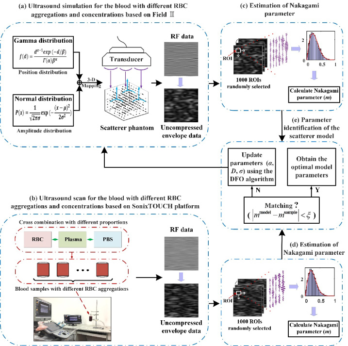
Flowchart of the simulation model for the blood with different red blood cell (RBC) aggregations and concentrations based on Field II. PBS is phosphate-buffered saline. ROI is region of interest. DFO is derivative-free optimization. 𝜉 is set to 10⁻³.

2.1. Scatterer model

The scatterer distribution model is commonly used to simulate the blood with various degrees of RBC aggregation. To establish a practical ultrasound scatterer model, the varying patterns of scatterer distribution adjusted by the position and scatterers’ amplitude are usually considered. Currently, a variety of point process models are available for describing the spatial distribution of scatterers, including the Neyman-Scott model [34], Quasi-Regular model [35], Gibbs-Markov model [36], and Cramblitt model [37]. Among these models, the Cramblitt one has been proven to be a flexible and realistic method, which is applicable to produce a scatterer distribution with varying density and spatial organization ranged from random to tightly clustered [38].

For the 1D Cramblitt model, scatterers are considered to be the points collected from a stationary renewal point process, i.e., a specific Poisson process. Accordingly, the original Cramblitt scatterer model [37] is formulated as given by: $\begin{eqnarray}s(x)=\mathop{\sum }_{i}a_{i}{\delta}(x-X_{i})\end{eqnarray}$ (1) where s (x) is the original 1D random scatterer, a _i and X _i denote the strength and position of the ith scatterer, respectively. According to Cramblitt and Parker [37], the Poisson point process can be defined in terms of statistics on the amount of the distance d between two consecutive points [37,38]. More specifically, if distance d obeys Gamma distribution, the probability density function (PDF) of a typical Poisson process f (d) with the scale parameter 𝛽 and shape parameter 𝛼 is given by [39]: $\begin{eqnarray}f(d)=\frac{d^{a-1}\exp (-d/{\beta})}{{\Gamma}({\alpha}){\beta}^{{\alpha}}}\end{eqnarray}$ (2) where 𝛼 > 0, 𝛽 > 0, and d > 0. The mean and variance of the space d are d = 𝛼𝛽 and 𝜎_d ² = 𝛼𝛽 ² = d ²∕𝛼, respectively. Therefore, the scatterer distribution can be equivalently described using shape parameter 𝛼 with the given mean distance d . For a fixed density, the scatterer distribution alters gradually from regular to random, further to aggregated, as the shape parameter decreases. More precisely: (i) when 𝛼 > 1, the scatterers are placed regularly and the point spacing has relatively low variance; (ii) when 𝛼 = 1, the scatterers are randomly distributed, which follow the exponential distribution; (iii) when 𝛼 < 1, the scatterers group in clusters and the point spacing shows high variance.

The normal distribution is used to tune the strength of the scatterers [40]. The PDF of a normal distribution p (x) with the random variable x is given by [41]: $\begin{eqnarray}p(x)=\frac{1}{\sqrt{2{\pi}}{\sigma}}\exp \left(-\frac{(x-{\mu})^{2}}{2{\sigma}^{2}}\right)\end{eqnarray}$ (3) where 𝜎 is the standard deviation, 𝜇 denotes the mean of the distribution. As a matter of notation, the normal distribution is often expressed as ${\mathcal{N}}({\mu},{\sigma}^{2})$ .

To develop a general 3D scatterer model while ensuring the isotropy of the scatterers, the above 1D scatterer distribution should be generalized into a 3D one, which can be realized by mapping its output to a 3D Hilbert space-filling curve [38,42]. This is due to the fact that the Hilbert space-filling curve is a continuous and nondifferentiable fractal curve, it is able to preserve the correlation of the adjacent scatterers in original space [42]. Details of this mapping algorithm can be found in the literature [43].

2.2. Statistic model for characterizing the echo envelope signals

The Nakagami distribution [48] (an approximation statistic model of the HK distribution) allows to characterize different organizations and distributions of scatterers in tissue [49], and has been demonstrated as a useful mathematical distribution to distinguish all ultrasound scattering conditions [50] with less computational complexity. According to Wu and Liao [31], the Nakagami distribution allows for the characterization of blood sample with different RBCs aggregation levels. The PDF of the Nakagami model f (R) calculated from the backscattered envelope R is defined as [51]: $\begin{eqnarray}f(R)=\frac{2m^{2}R^{2m-1}}{{\Gamma}(m){\Omega}^{m}}\exp \left(-\frac{m}{{\Omega}}R^{2}\right)U(R)\end{eqnarray}$ (4) where 𝛤(⋅) is the Gamma function, U (⋅) is the unit step function, m and 𝛺 are the shape and scaling parameters, respectively. The scaling parameter 𝛺 is estimated as: $\begin{eqnarray}{\Omega}=E(R^{2})\end{eqnarray}$ (5) and the shape parameter m can be formulated as: $\begin{eqnarray}m=\frac{[E(R^{2})]^{2}}{E[R^{2}-E(R^{2})]^{2}}\end{eqnarray}$ (6) where E (⋅) stands for the expectation operator. The flexibility of the Nakagami distribution can be understood by noting that m controls the PDF in Eq. (4) to approximate different distributions: (i) m < 1, the PDF represents a pre-Rayleigh or generalized Rician distribution; (ii) m = 1, the PDF is a function of the Rayleigh distribution; (iii) m > 1, the distribution of the backscattered-signal envelope follows the post-Rayleigh or Rician distributions. Owing to its data-driven nature in addition to the ability of fitting a wide variety of distributions, the Nakagami statistics are adopted in this work as the indicators to evaluate whether the simulation mode matches the blood sample.

2.3. Strategy of setting the initial values for the simulation model

As shown in Fig. 1(a), we use the Gamma distribution and normal distribution to control the position and strength of the scatterers, respectively. To find the eligible model parameters conforming to the in-vitro experiment ones quickly and automatically, parameters (𝛼, D, 𝜎) of the proposed model will be initialized under the guidance of the following strategies:

(i) Studies have shown that the value of parameter D has important effect on the scatterer distribution, i.e., increasing the value of parameter D will produce a denser distribution in space [39]. Accordingly, different patterns of hematocrits can be simulated by altering the value of parameter D of the scatterer model. Therefore, to simulate various hematocrits that cover most of the clinical situations (in normal blood flowing through human vessels, HCT ∈ [35%, 55%]), we first set the scatterer model under a low density with D = 1, and then increase its value to match higher hematocrits in clinical practice.

(ii) As described in Section 2.1., when the value of D is fixed, the scatterer distribution alters gradually from regular to random, and further to aggregated as the shape parameter 𝛼 decreases. Specially, when 𝛼 = 1, the scatterers are randomly distributed in space [40], which is consistent to the distribution of RBCs in normal blood flow. Therefore, before optimizing the model parameters, we chose to set 𝛼 = 1 as the initial state of the model to construct a non-aggregated RBCs pattern, and then continue to reduce the value of 𝛼 to approach the aggregated RBCs pattern by adjusting the position distribution of scatterers in the space.

(iii) The scatterers in the blood model represent RBCs, which is in agreement with the clinical observations that RBCs may behave as chief scattering sources as a collection of independent stochastic cells [52]. Moreover, with a fixed hematocrit, the ultrasonic echo intensity of the blood is related to the degree of RBC aggregation (the more the RBCs aggregated, the higher the energy intensity). According to Jensen and Svendsen [30], scatterers with different amplitudes are used for the ultrasound simulation of blood and their distribution follows a normal distribution ${\mathcal{N}}({\mu},{\sigma}^{2})$ . In other words, we can generate a series of normal distributions with a given 𝜇 and different value of 𝜎, which can be used to model the varied amplitude of the RBC aggregation. Therefore, we chose 𝜇 = 0 and 𝜎 = 1 as the initial setting of the amplitude to model the amplitude of the blood with non-aggregated RBCs. Then, for the blood with different level of RBCs aggregation, the energy increment that caused by the clustering of scatterers will be simulated by increasing the value of 𝜎 further with the parameter 𝜇 remains equal to 0 [53].

Based on the analysis presented above, we propose to set as 𝛼 = 1, D = 1, 𝜇 = 0, and 𝜎 = 1 at the first stage of the method. Then by leveraging the DFO algorithm, the model will quickly converge to the eligible solutions.

2.4. Parameter identification of the scatterer model

Before the proposed model can be utilized for forecasting future RF signals, the model parameters need to be calibrated such that simulation results match with the in-vitro history. To determine the parameters of the blood model corresponding to different RBC aggregations and concentrations, Nakagami parameters of the envelope signals simulated from different distributions associated with the scatterer model are calculated and matched with those of the results based on in-vitro experiments. Such procedures of the parameter identification are described in Fig. 1(e).

According to Section 2.1., the scatterer distribution of the proposed model depends on three parameters (𝛼, D, 𝜎). Therefore, the error statistic |m ^model − m ^sample| can be written as a function of these three parameters, i.e., f (𝛼, D, 𝜎). Since our goal is to minimize the error of the Nakagami parameter between the simulated and in-vitro RF signals, the problem of parameter identification is essentially a general optimization problem of the form $\begin{eqnarray}\min _{{\Theta}}f({\alpha},D,{\sigma})\end{eqnarray}$ (7) where ${\Theta}\in \mathbb{R}^{3}$ represents the feasible value range of parameters (𝛼, D, 𝜎). However, due to our model output is the result obtained from a series of simulations, the objective function f defining on set 𝛩 is provided as black-box in the sense that the way to obtain a function value from a given parameter set cannot be provided in an analytical way. As a result, the gradient of the objective function with respect to unknown model parameters is quite difficult to obtain, and this can limit the use of gradient-based optimization methods.

To address the above issue, we apply the MADS [32] optimization algorithm in our parameter identification procedure. A detailed description of this algorithm can be found in the literature [32]. By gradually reducing the error of the Nakagami parameter between the in-vitro experiments and simulations using the above MADS algorithm, the eligible parameters of the developed scatterer model for the investigated blood sample are determined as given by x ^k+1 = (𝛼^k+1, D ^k+1, 𝜎^k+1) = (𝛼⁰, D ⁰, 𝜎⁰), where k is the iteration counter. For convenience, we will refer to the final parameter (𝛼^k+1, D ^k+1, 𝜎^k+1) as (𝛼^f, D ^f, 𝜎^f) in the following sections.

For the investigated blood samples, according to our test, the magnitude of 𝛼 associated with the developed model is about 10 times smaller than D and 𝜎. Therefore, the spanning matrix is designed as: $\begin{eqnarray}D=\left[\begin{array}{@{}cccccc@{}}1 & 0 & 0 & -1 & 0 & 0\\ 0 & 10 & 0 & 0 & -10 & 0\\ 0 & 0 & 10 & 0 & 0 & -10\end{array}\right]\end{eqnarray}$ (8) despite the fact that previous literature [32] recommends the use of unit column vectors in the expansion matrix.

In this work, after comprehensively considering the accuracy and speed for RBC modelling, the selected parameter configuration is Δ^min = 0.01 and Δ^stop = 0.005, where Δ^min and Δ^stop denote the minimum mesh and mesh stopping tolerance, respectively. The remained parameters are set to their default values, i,e., Δ⁰ = 1 and 𝜏 = 0.5 [32 ].

3. Experiments

3.1. Blood sample preparation

The fresh porcine blood was bought from a local slaughter house, which was subsequently anti-coagulated with heparin injection (10 g/L), and filtered through a sponge to remove impurities (such as hair and fatty tissue). To obtain autologous RBCs and plasma, whole blood was centrifuged (TD4Z, Guangfeng Technology Co., Ltd, Tianjin, China) at 2000 rpm for 10 min. Thereafter, the collected RBCs were washed 2 times with the phosphate-buffered saline (PBS, PH 7.4). In order to simulate RBC aggregation with different levels of HCT, we prepared various blood samples by remixing the RBCs with a certain volume of autologous plasma and PBS, which is essentially a three-step process: (i) Five different concentrations of PBS-plasma solutions (the proportion of plasma in PBS-plasma solution is 15%, 30%, 45%, 60%, and 75%) were prepared by diluting the plasma with PBS, and each of these solutions was subdivided equally into three groups. (ii) For each PBS-plasma solution, RBCs were added to the three groups respectively to construct blood samples with three different hematocrits (HCT = 20%, 40%, and 60%). (iii) A total of 15 kinds of blood samples with different HCTs and plasma concentrations (PC) were obtained and injected into the corresponding upright polypropylene infusion bags. To simplify nomenclature, the blood samples are labeled as HCT_xPC_y, where x is assigned to 20, 40 and 60, and y is marked with 15, 30, 45, 60 and 75, which represent the percentage concentration of RBC and plasma, respectively. Finally, ten copies of each blood sample were prepared in the same way and all experiment were conducted at a consistent room temperature of 25 °C.

Moreover, to evaluate the aggregation patterns of the RBCs, these reconstituted blood samples were sampled and observed with a microscope (SAGA, SG100-2A41L-A, Shenying Optics, Co., Ltd, Suzhou, China) after standing for 5 minutes.

3.2. Ultrasound data acquisition in-vitro

For each blood sample, 10 independent scans were performed to acquire the B-mode images and backscattered RF signals using the SonixTOUCH ultrasound platform (SonixTOUCH Ultrasonix Medical Corporation, Burnaby, British Columbia, Canada) with a L40-8/12 linear-array transducer. Figure 2 shows the experimental configuration of data acquisition. As shown in Fig. 2(a), the bracket preforms the task of fixing the infusion bag that contains the reconstituted blood sample. After applying the ultrasonic coupling agent to the probe surface evenly, the probe was set to the bracket with the surface fitting to the bag to collect the backscattered ultrasonic RF echo signals. Figure 2(b) lists the ultrasonic scanning parameters used in the SonixTOUCH ultrasound system. The RF signals were digitized at a sampling frequency of 40 MHz and the acquisition time lasted 5 s for each sample set.

Fig. 2.

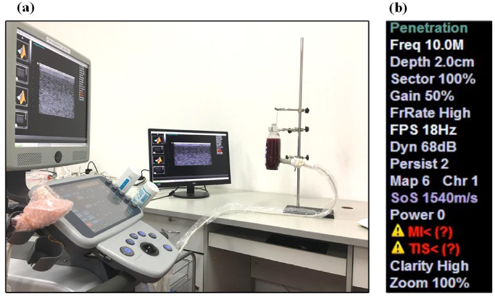
Configuration for the acquisition of the RF signals and the B-mode images in the in-vitro experiment.

3.3. Ultrasound simulation of blood based on Field II

In ultrasound simulation, numerical phantoms for blood with various levels of RBC aggregations were generated, where the initial values of parameters (𝛼, D, 𝜎) were set according to the strategy presented in Section 2.3.. Then, to obtain the eligible model parameters consistent with the in-vitro ones, the MADS optimization algorithm was subsequently adopted to search the solutions.

In this simulation, a certain number of scatterers simulating the RBCs were filled in a cube with the size of 6 mm × 6 mm × 6 mm. The backscattered RF data of the scatterer models was generated using Field II. Table 1 provides a brief summary of the simulation parameters, among which, the acoustic parameters are the same as those used in the in-vitro experiment. Notably, the distance between the transducer face and the surface of the numerical phantom was 20 mm. Based on the above configuration, the scatterer model of each set of parameters (𝛼, D, 𝜎) can be simulated to obtain the corresponding RF signals and B-model images.

Table 1
The ultrasonic simulation parameters used in Field II

Parameter name Values

Acoustic parameters Center frequency (MHz) 10

Sampling frequency (MHz) 40

Speed of sound (m/s) 1540

Wavelength (m) 1.54 × 10⁻⁴

Parameters for the linear array transducer Physical elements 512

Active elements 64

Elements width (m) 1.54 × 10⁻⁴

Elements height (m) 0.005

Fixed focal point (m) [0, 0, 0.02]

Scanning lines 50

Parameter name	Values
Acoustic parameters	Center frequency (MHz)	10
	Sampling frequency (MHz)	40
	Speed of sound (m/s)	1540
	Wavelength (m)	1.54 × 10⁻⁴
Parameters for the linear array transducer	Physical elements	512
	Active elements	64
	Elements width (m)	1.54 × 10⁻⁴
	Elements height (m)	0.005
	Fixed focal point (m)	[0, 0, 0.02]
	Scanning lines	50

3.4. Model parameters acquisition and validation

3.4.1. Model parameters acquisition

According to the descriptions in Sections 3.1. and 3.2., ten copies of each blood sample were prepared during the in-vitro experiment, and for each copy we scanned 10 times independently and collected 10 raw RF signals. Then for each RF data, we randomly selected 100 ROIs in order to obtain the corresponding envelope signals for fitting the Nakagami parameter. Specially, we first select 10 frames of RF data from each raw RF data, and then, 10 ROIs are randomly selected from each frame of RF data with 10 RF scan lines (each scan line contains 100 sample points). As a result, totally 1000 sets of independent ROIs (envelope signals) would be obtained for each kind of the blood sample.

To obtain the parameters of the model, for each kind of the blood sample, all the ROIs data (1000 sets) from the in-vitro experiment were used. The specific process is as follow: (i) The envelope signals of the 10 RF scan lines (one ROI) were obtained using the Hilbert transform and then connected end-to-end to form a 1D data [35,36]. (ii) The 1D connected envelope signal was estimated using the Nakagami distribution without the log-compression. Without loss of generality, we calculated the Nakagami parameter m _i ^sample (where i = 1,2, …,1000) corresponding to each region of interest separately and then treated their least squares solutions as the representative parameter m ^sample of the current blood sample, namely $\begin{eqnarray}m^{\text{sample}}=LS\{(m_{1}^{\text{sample}},m_{2}^{\text{sample}},\ldots ,m_{1000}^{\text{sample}})\}\end{eqnarray}$ (9) where $LS\{\cdot \}$ stands for the least squares operator. After obtaining the quantitative statistic (Nakagami parameter) of the sample, the next step was to tune the parameters of the scatterer model (𝛼, D, 𝜎) so that its calculated quantitative statistics approximate that of the sample. By initializing the parameters as (1,1,1), the Field II was used to construct the scatterer model for simulating the corresponding RF data. Similarly, 1000 sets of ROIs were randomly generated from the simulation model, to yield an initial Nakagami parameter m ^model. It should be noted that when the model parameters are fixed, the copy of this model is still itself. Therefore, we performed 100 independent scans of the model at each time, and then extracted 10 times for each scan to obtain 1000 sets of ROIs. Finally, the relative error g (𝛼, D, 𝜎) between m ^model and m ^sample was calculated on basis of the following equation: $\begin{eqnarray}g({\alpha},D,{\sigma})=|m^{\text{model}}-m^{\text{sample}}|.\end{eqnarray}$ (10)

If g does not satisfy the error tolerance (g < 𝜉, where 𝜉 is set to 10⁻³ throughout this work), the MADS algorithm would be triggered to guide us to adjust the parameters (𝛼, D, 𝜎) until the objective function g converged to an acceptable minimum. Consequently, this process was stopped after we obtained a set of eligible parameters (𝛼^f, D ^f, 𝜎^f) for the proposed scatterer model.

3.4.2. Method validation

To validate the effectiveness of the proposed model, a 10-fold cross-validation strategy was performed. For each kind of blood sample, we randomly divided the corresponding RF data from the in-vitro experiment to 10 folds. Then we trained the model on 90% of the RF data and tested (validated) it on the remaining 10%. This procedure has been repeated 10 times for all 10 portions of the data, thus the accuracy of the model parameters was reported as an ensemble over the 10 training-testing experiments. Notably, each of the 15 kinds of those reconstituted static blood samples in the in-vitro experiment was validated using the 10-fold cross-validation strategy.

Fig. 3.

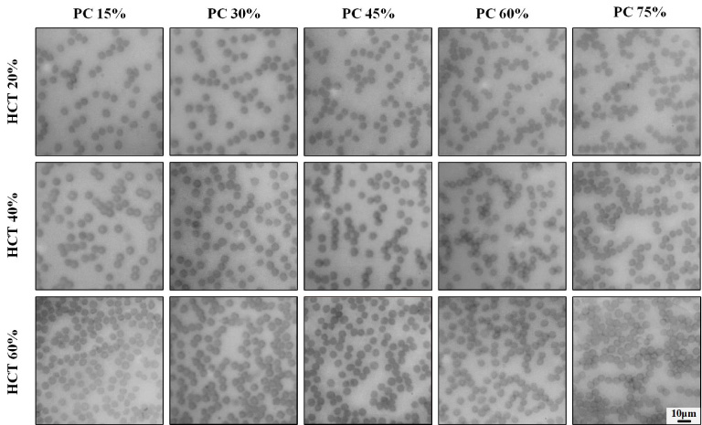
Microscope images for the blood samples with 15 kinds of RBC aggregations. The scale bar denotes 10 μm.

In each fold, the parameters (𝛼^f, D ^f, 𝜎^f) corresponding to the 90 sets of training RF data from the in-vitro experiment were obtained using the same operation described in Section 3.4.1.. Then, the scatterer model of the parameters (𝛼^f, D ^f, 𝜎^f) was construct and simulated 10 times to generate the 10 RF data. Similar to Section 3.4.1., we next selected 10 ROIs randomly from each RF data to obtain 100 sets of tested envelope signals. After quantifying those envelope signals using the Nakagami distribution, 100 sets of Nakagami parameter $(m_{j}^{\text{model}})_{j=1}^{100}$ corresponding to the proposed model were finally obtained. Similarly, the Nakagami parameter of the remaining 10% data (also 100 sets of ROIs in total) from the in-vitro experiment was calculated as $(m_{j}^{\text{sample}})_{j=1}^{100}$ . Finally, we proposed to use the RMSD between the Nakagami parameter of the sample and those from the model to quantify the accuracy of the method. The RMSD formulation of m is given by: $\begin{eqnarray}\text{RMSD}^{m}=\sqrt{\frac{1}{100}\mathop{\sum }_{j=1}^{100}(m_{j}^{\text{model}}-m_{j}^{\text{sample}})^{2}}.\end{eqnarray}$ (11)

Accordingly, the lower the value of RMSD^m, the higher accuracy of the trained model. It should be noted that the leave-10%-out training-testing process has been repeated for 10 rounds to ensure that all 10 portions of the data were used for testing. Therefore, the performance of the proposed method was finally evaluated by the mean and standard deviation of the RMSD values from the 10 rounds validation for m.

All the above simulation and performance evaluation were conducted with the operating system of Windows 10 and the software platform of Matlab R2018a (The MathWorks, Inc., Natick, MA, USA), under Intel(R) Xeon(R) CPU (W-2125) 4.0 GHz and 32 GB memory.

Fig. 4.

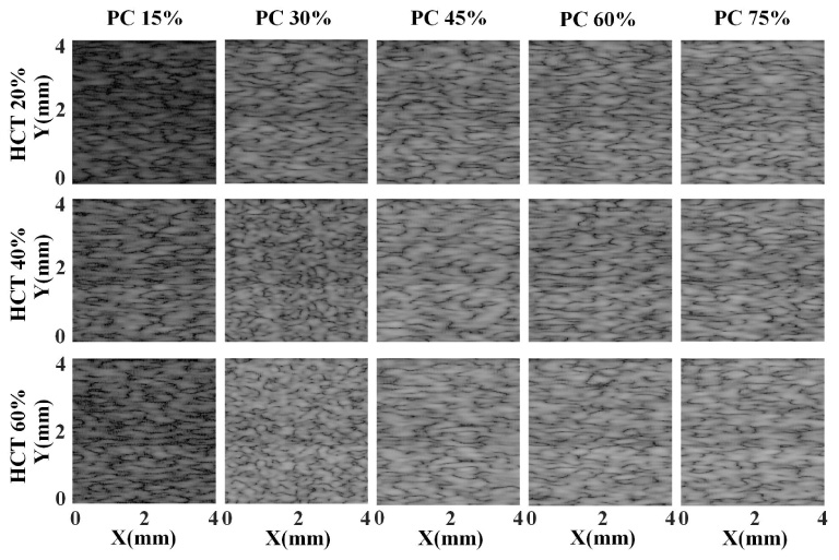
B-mode images for the blood samples with 15 kinds of RBC aggregations.

4. Results

4.1. Microscopy images of RBC suspensions

Typical microscope images of the remixed blood samples with five different plasma concentrations at three hematocrit levels are shown in Fig. 3. It is observed that: (i) RBCs give rise to increasing aggregation as the plasma concentration increases. (ii) With the increase of the hematocrit, RBCs become clustered progressively.

4.2. Ultrasonic characterization of RBC suspensions

After the interpolation and logarithmic compression, typical B-mode images of the collected RF data corresponding to the blood samples with various RBC aggregation levels are yielded and depicted in Fig. 4. Accordingly, we make following observations from this figure: (i) When the hematocrit level is fixed, higher echogenicity can be observed in the B-mode image with higher plasma concentration than that with lower plasma concentration. (ii) With the same concentration of plasma, the higher the RBC density, the higher echogenicity of the B-mode image. (iii) The texture in the images becomes denser as more plasma and RBCs are combined into the PBS. Overall, the above observations suggest that the increase of the aggregation level of RBCs is capable to enhance the echogenicity intensity, which is consistent with the previous studies [7].

Figure 5 shows the statistical histograms and fitted curves of the envelope signals demodulated from the ultrasound B-images shown in Fig. 4, where the statistical histograms reflect the distributions of ultrasonic-echoed envelope data while the red fitted curves represent the characteristic curves estimated with the Nakagami distribution. From this figure, it can be found that:

(i) When PC = 15%, the fitted curves of ultrasonic-echoed envelope data corresponding to three hematocrits are close to Rayleigh distribution. We also notice that as the increase of PC, the fitted curves approach the Pre-Rayleigh distribution or K distribution gradually, where the curves corresponding to PC = 75% are most representative.

(ii) Different RBC densities also lead to different fitted distributions of the envelope signals. More specifically, as the PC increases from 15% to 75%, the higher the RBC density, the more obvious the change in distribution (from Rayleigh to Pre-Rayleigh distribution) of the ultrasonic-echoed envelope data shown in these images.

Fig. 5.

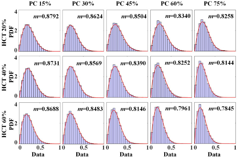
The statistical histograms and Nakagami fitted curves for the envelope signals of the blood samples with 15 kinds of RBC aggregations.

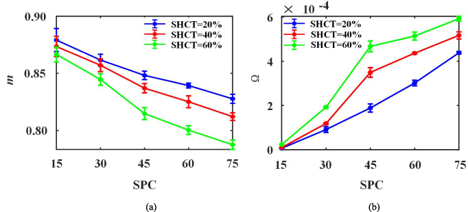
According to Section 3., totally 100 sets of independent raw RF data have been obtained for each kind of the blood suspension. To demonstrate that the Nakagami parameter is indeed capable of reflecting the red blood cell aggregation of the suspension, the means and standard deviations (STDs) of m corresponding to each of blood samples were calculated and plotted in Fig. 6(a), where each statistic was obtained from 1000 independent ROIs of the raw RF data. In this figure, the curves related to three different hematocrit levels (HCT 20%, HCT 40% and HCT 60%) are plotted by blue, red and green curves, respectively. It is concluded that the Nakagami parameter m decreases with increasing plasma concentration.

More specifically, from Fig. 6(a), we can see that: as the percentage of plasma rising, the blue curve (HCT 20%) descends gently with a relatively slow slope; while, the curves of m plotted in the red curve (HCT 40%) and the green curve (HCT 60%) fall at faster rates, where the green curve drops most obviously. Based on the observation, we concluded that the distribution of the envelope signal, corresponding to a relatively higher hematocrit level, possesses a faster alteration from Rayleigh to Pre-Rayleigh distribution as the plasma concentration increases, which is consistent with the results shown in Fig. 5.

Fig. 6.

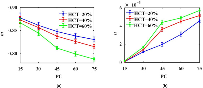
The means and STDs curves of Nakagami parameters of the blood samples with 15 kinds of RBC aggregations.

To observe the variation of the echo strength of the blood samples, the envelope signals demodulated from all acquired raw RF data are normalized and then quantized using the Nakagami scaling parameter 𝛺, where the results are shown in Fig. 6(b). It is clear that with the PC grows, the green curve shows the fastest growth of 𝛺, the blue curve shows the smoothest trend, while the red curve reaches a compromise. Among all three curves, 𝛺 of HCT 20% is far smaller than the ones of HCT 40% and HCT 60%, and 𝛺 of HCT 40% approaches the one of HCT 60%, but the former is always lower than the latter. The results illustrate that the echo strength can be enhanced by increasing of the concentration of RBC and plasma.

Finally, by combining Fig. 6(a) with Fig. 6(b), we observe that the minimum m and the maximum 𝛺 appear simultaneously at HCT = 60%, PC = 75%, which corresponds to the most aggregated RBCs suspension. In short, the rise of the aggregation level not merely alters the shape parameter m, but also yields the higher echogenicity.

4.3. Distributions of the simulated scatterer model

In order to explore the effect of model parameters (𝛼, D, 𝜎) on the distribution of the simulated echo envelope signals, the isotropic scatterer distribution models based on different shape and density parameters of Gamma distribution as well as the standard deviation of normal distribution are built and simulated. Specially, a set of typical examples are shown in Fig. 7 with the size of 4 mm × 4 mm. The following observations can be drawn from the figure.

(i) With a fixed D, the randomicity of scatterers is better when the parameter 𝛼 is higher. For instance, 𝛼 = 1 means that the scatterers are randomly distributed in the space, while 𝛼 = 0.01 means a more clustered set of the scatterers. Notably, the similar observation can be found in previous study [39].

(ii) When 𝛼 is fixed, a higher density parameter D leads to a denser and more aggregated scatter distribution, which is consistent to the mechanism of the Cramblitt model [31].

(iii) With the increase of 𝜎, the gray values of the scatterer model increase dramatically, which indicates that the scattering intensity is enhanced. While, the variation of 𝜎 has nothing to do with the scatterers spatial distribution.

Fig. 7.

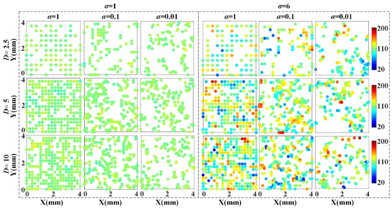
The scatterer distributions from the Gamma distribution with different values of shape parameter and density parameter as well as the normal distribution with different standard deviation 𝜎.

4.4. Ultrasonic characteristic of scatterer model

Figure 8 shows the B-model images corresponding to the scatterer distributions in Fig. 7. In this figure, we can observe that: (i) With a lower 𝛼, the clustered scatterer distribution in Fig. 7 produces tighter speckles with a higher echogenicity. Especially for 𝛼 = 0.01, the speckles in the B-mode images are densest and brightest with a fixed D. (ii) For a given 𝛼, a denser and more aggregated scatterer distribution shown in Fig. 7 (with a higher density parameter D) also leads to higher echogenicity in the corresponding B-mode images. (iii) In case of 𝜎 = 6, specks in B-mode images are more brighter than that of 𝜎 = 1, which indicates that a higher value of 𝜎 can generate a higher scattering intensity.

Fig. 8.

B-mode images for the scatterer models with different model parameters.

Fig. 9.

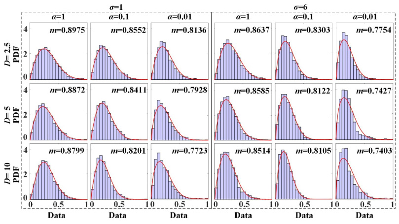
The statistical histograms and Nakagami fitted curves for the envelope signals of the scatterer models with different model parameters.

To depict the distribution characteristics of the simulated ultrasonic RF signals, we also perform the probability distribution analysis on the envelope signals corresponding to the images of Fig. 8, where the statistical histograms and Nakagami distribution based fitting curves are shown in Fig. 9. As can be seen in this figure, the simulated envelope signals from the scatterer model with different values of 𝛼, D and 𝜎 present different histograms and distributions. In specific: (i) with the decrease of 𝛼, there is an obvious transformation of the fitted curves from Rayleigh to Pre-Rayleigh distribution. (ii) the change in distribution becomes more pronounced as the increase of D and 𝜎. Therefore, it is concluded from the above analysis that the distribution characteristic of the envelope signal is consistent with that shown in Fig. 6.

Similar to Fig. 6, in order to demonstrate that the adjustment of the simulation model parameters can also be reflected on Nakagami parameter, a series of Nakagami results corresponding to different simulation parameters are obtained here. Among which, the shape parameter is represented by the base-10 logarithm (log₁₀𝛼), and its values are set to 0, −0.25, −0.5, −0.75, −1, −1.25, −1.5, −1.75 and −2, respectively. Moreover, the density parameter is set to 2.5, 5 and 10, and the standard deviation is valued by 1, 3 and 6. After simulation based on the Field II platform, the RF data corresponding to different parameter configurations are acquired and then a normalized solution is performed. More precisely, for each set of simulation parameters, 1000 independent ROIs are randomly selected from the simulated RF data to obtain the Nakagami parameters, which uses the same operations descripted in Section 4.2.. The STDs of m and 𝛺 corresponding to different simulation parameters were calculated and shown in Fig. 10.

Fig. 10.

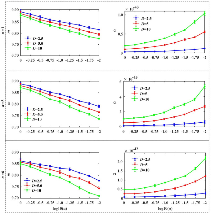
The means and STDs curves of Nakagami parameters of the scatterer models with various kinds of distributions.

In this figure, the curves corresponding to density parameters D = 2.5, D = 5 and D = 10 are figured by blue, red and green, respectively. As shown in this figure, parameters D, 𝛼 and 𝜎 have great impact on the values of Nakagami parameter m and 𝛺, More specifically:

(i) For a fixed density parameter, a gradual decrease of m is noticed between log₁₀𝛼 = 0 and log₁₀𝛼 = −2, which indicates that the scatterers distribution has evolved from Rayleigh into Pre-Rayleigh distribution. Besides, the value of m corresponding to D = 10 drops at the fastest rate, which is followed by the curves of D = 5 and D = 2.5 in turn.

(ii) With a given D, there is a significant upward trend of the scaling parameter 𝛺 as the value of 𝛼 decreases. Specifically, for the three different density parameters (D = 2.5, D = 5 and D = 10), the bigger the value of D shows the faster growth of 𝛺.

(iii) When log₁₀𝛼 = −2, D = 10 and 𝜎 = 6, the values of 𝛺 and m reach the maximum and minimum values, respectively. In summary, the model with a smaller log₁₀𝛼 and bigger D would yield higher echo energy, and the distribution of the corresponding envelope signal is also closer to the Pre-Rayleigh distribution, which is in agreement with the results of in-vitro experiments described in Fig. 6.

4.5. Results of the proposed model

4.5.1. Final model parameters and its ultrasonic characteristics

According to the experimental configuration in Section 3., we obtained the final model parameters corresponding to the typical 15 kinds of blood samples based the proposed modeling method. Table 2 shows the values of the final model parameters (𝛼^f, D ^f, 𝜎^f), from which the values of shape parameter 𝛼, density parameter D of Gamma distribution, and the standard deviation 𝜎 of the normal distribution for scatterer distribution of each blood sample are listed, respectively. From this table we observe that: (i) For a given hematocrit of blood sample, with the plasma concentration increasing, there is a smaller value of 𝛼 and a larger value of 𝜎. However, the increase of plasma concentration in the blood sample has no significant effect on D. (ii) For the blood samples that with the same concentration of plasma, the higher the hematocrit, the bigger the value of D. Moreover, there is a relatively large value of 𝜎 appears in the blood sample with a high plasma concentration. While, the effect of the increase of plasma concentration on 𝛼 is not obvious. Based on the above analysis, we conclude that these model parameters should be adjusted simultaneously to obtain the simulation parameters for the blood sample with different HCTs and PCs.

Table 2
The optimal model parameters (𝛼⁰, D ⁰, 𝜎⁰) corresponding to the mixed blood samples

Blood samples Values of the model parameters

𝛼 D 𝜎

HCT₂₀ PC₁₅ 0.55 2.2 1.2

HCT₂₀ PC₃₀ 0.13 2.4 3.4

HCT₂₀ PC₄₅ 0.05 2.2 4.3

HCT₂₀ PC₆₀ 0.02 2.6 4.5

HCT₂₀ PC₇₅ 0.01 2.3 4.8

HCT₄₀ PC₁₅ 0.55 5.1 1.5

HCT₄₀ PC₃₀ 0.12 4.7 4.0

HCT₄₀ PC₄₅ 0.04 5.2 4.3

HCT₄₀ PC₆₀ 0.02 5.2 4.5

HCT₄₀ PC₇₅ 0.01 5.3 5.3

HCT₆₀ PC₁₅ 0.53 9.0 1.9

HCT₆₀ PC₃₀ 0.11 10.2 3.7

HCT₆₀ PC₄₅ 0.04 11.7 4.5

HCT₆₀ PC₆₀ 0.02 10.8 4.7

HCT₆₀ PC₇₅ 0.01 10.5 5.4

Blood samples	Values of the model parameters
HCT₂₀ PC₁₅	0.55	2.2	1.2
HCT₂₀ PC₃₀	0.13	2.4	3.4
HCT₂₀ PC₄₅	0.05	2.2	4.3
HCT₂₀ PC₆₀	0.02	2.6	4.5
HCT₂₀ PC₇₅	0.01	2.3	4.8
HCT₄₀ PC₁₅	0.55	5.1	1.5
HCT₄₀ PC₃₀	0.12	4.7	4.0
HCT₄₀ PC₄₅	0.04	5.2	4.3
HCT₄₀ PC₆₀	0.02	5.2	4.5
HCT₄₀ PC₇₅	0.01	5.3	5.3
HCT₆₀ PC₁₅	0.53	9.0	1.9
HCT₆₀ PC₃₀	0.11	10.2	3.7
HCT₆₀ PC₄₅	0.04	11.7	4.5
HCT₆₀ PC₆₀	0.02	10.8	4.7
HCT₆₀ PC₇₅	0.01	10.5	5.4

Similar to Fig. 6, corresponding to the blood sample in the in-vitro experiment, the scatterer model of each set of final parameters is constructed and simulated to obtain 100 sets of RF data. Then, the RF data of all 15 kinds of blood model are obtained and uniformly normalized. Accordingly, for each set of final parameters, 1000 independent ROIs are randomly selected from its normalized RF data and then fitted using the Nakagami distribution to obtain parameters m and 𝛺. The means and STDs curves of the Nakagami parameters are shown in Fig. 11. From the graph, we can see that the variation of Nakagami parameters show consistent tendency with that of Fig. 6, i.e., m decreases with increasing plasma concentration, while 𝛺 shows an opposite character.

Fig. 11.

The means and STDs curves of Nakagami parameters of the scatterer models with 15 kinds of distributions.

4.5.2. Validation results

According to Section 3.4.2., the accuracy of the model parameters is validated using a 10-fold cross-validation strategy, and the means and STDs of the RMSD values for parameter m from 10 rounds of validation are calculated. For different hematocrits and plasma concentrations, the scatterer model of the blood sample can be constructed and simulated accurately with lower RMSDs (The means and STDs of the RMSDs of m between the preset samples and the measured ones from the simulation model for five levels of RBC aggregation are 0.22 ± 0.0033, 0.18 ± 0.0016, 0.13 ± 0.0018, 0.13 ± 0.0012 and 0.10 ± 0.0029 respectively). The above experimental results support that our proposed method can be used to model the blood sample with different RBC aggregations effectively.

5. Discussion

The investigation of aggregation of RBCs is a promising direction for better understanding the pathophysiological process of diseases, clinical diagnosis and drug therapy [7,8]. Previous studies inspire us to select a numerical simulation model to understand the scattering process of blood. However, there is a significant limitation that the formation of truly random point configurations is ignored (for clustered configurations, the strong short-range repulsive potential introduces regular structure within the clusters) and these models do not consider the effect of RBC aggregation under different HCTs and PCs.

To address the above problem, we develop a flexible ultrasound model for blood simulation by extending one of our conference paper. In the present study, the procedures of the method are improved and formulated precisely in mathematical terms, and the analyses are extended with more kinds of hematocrits and plasma concentrations (HCT levels of 20%, 40% and 60%, as well as plasma concentrations of 15%, 30%, 45%, 60% and 75%). Additionally, we improve the original (manual) parameter identification procedure for the blood model corresponding to different RBC aggregation suspensions by using the MADS optimization algorithm. Moreover, compared with our previous work [31], a 10-fold cross-validation experiment is performed in this work to validate the effectiveness of the proposed model.

After acquiring the eligible model parameters, the scatterer model conforming to blood samples in-vitro is established. Consequently, the corresponding ultrasonic (statistical) characteristics of the envelope signals about the simulated RF echo signals, i.e., B-mode images, statistical histograms and fitted curves, Nakagami parameters, can be obtained. The results presented in Section 4.5. indicate that, with the increasing cluster degree of the scatterer, the distribution of the simulated envelope signals alters from Rayleigh to Pre-Rayleigh distribution, with the scattering intensity being enhanced synchronously. Furthermore, from Fig. 3 to 5, we also conclude that the variation of model parameters has significant impact on the characteristics of the scatterer model. It means that the proposed simulation model is an effective method for modeling the blood with various HCTs and PCs.

Finally, we perform a 10-fold cross-validation strategy to assess the accuracy of the final parameters of the model. Values of RMSDs show that the results for the aggregating scatterer model based on the final model parameters are in good agreement with these in-vitro ones presented in Section 4.2.. On the other hand, by simply defining the appropriate model parameters, the properties of the scatterers can be modeled associated with different distribution characteristic, which is flexible and convenient.

However, it should be noted that, in our model, there is no attempt to design the RBCs as spheres, biconcave or flexible objects. These characteristics promote the formation of rouleaux to some extent, which cannot be reflected with our model. In addition, the blood sample tested in the experiments is reconstituted static blood samples rather than the flowing blood in-vivo. Besides, although we have only estimated the parameters of 15 kinds of typical blood samples in this study, and the model parameters corresponding to other types of blood sample can also be obtained using the same modeling method in our work.

We highlight that there are two parameters associated with the Nakagami distribution (m and 𝛺 in Eq. (4)). However, due to the fact that the echo intensity of blood collected from the ultrasound machine is different in magnitude from the ones of simulated model, the parameter 𝛺 cannot be used in the process of determining model parameters since it is difficult to find a suitable standard for normalization. Therefore, we only select the shape parameter m to characterize the statistic distribution of the envelope signal obtained from the blood sample or simulation model. Our results show that the selected parameter m is capable of providing a good fit to the histogram of the envelope signal, which performs an accurate distinguishment among different RBC aggregated degrees under a same hematocrit.

6. Conclusion

A flexible scatterer model has been built using the Hilbert space-filling curve. Accordingly, the eligible model parameters corresponding to 15 kinds of typical RBC suspension samples have been estimated. Finally, this work has performed a 10-fold cross-validation experiment, to validate the effectiveness of the proposed model (where, for the three hematocrit levels of 20%, 40% and 60%, the mean and standard deviation of the RMSDs of the Nakagami parameter m between the preset samples and the measured ones from the simulation model for five plasma concentrations are 0.22 ± 0.0033, 0.18 ± 0.0016, 0.13 ± 0.0018, 0.13 ± 0.0012 and 0.10 ± 0.0029 respectively). In conclusion, the proposed ultrasound simulation model can be used to provide a realistic data source in the ultrasonic blood characterization field and to evaluate the performance of the ultrasound-based methods for detection and classification of RBC aggregation.

Footnotes

Acknowledgements

This work was supported by grants from the National Natural Science Foundation of China (No. 81771928), the Yunnan Fundamental Research Projects (No. 202101AS070031) and University Key Lab of Electronic Information Processing of High Altitude Medicine, Yunnan Province.

Conflict of interest

None to report.

Ethical declaration

Approval was obtained from the Ethics Committee of Medical School, Yunnan University. All insti tutional and national guidelines for the care and use of laboratory animals were followed.

References

Franceschini

Saha

R.K.

and Cloutier

, Comparison of three scattering models for ultrasound blood characterization, IEEE T Ultrason Ferr 60(11) (2013), 2321–2334. doi:10.1109/TUFFC.2013.6644736.

Saha

R.K.

and Cloutier

, Monte Carlo study on ultrasound backscattering by three-dimensional distributions of red blood cells, Phys Rev E 78(6) (2008), 061919. doi:10.1103/PhysRevE.78.061919.

Nam

K.H.

Yeom

, Simultaneous measurement of red blood cell aggregation and whole blood coagulation using high-frequency ultrasound, Ultrasound Med Biol 38(3) (2012), 468–475. doi:10.1016/j.ultrasmedbio.2011.11.013.

F.T.

Armstrong

J.K.

Tripette

, A local increase in red blood cell aggregation can trigger deep vein thrombosis: Evidence based on quantitative cellular ultrasound imaging, J Thromb Haemost 9(3) (2011), 481–488. doi:10.1111/j.1538-7836.2010.04164.x.

Tripette

Nguyen

L.C.

Allard

, In vivo venous assessment of red blood cell aggregate sizes in diabetic patients with a quantitative cellular ultrasound imaging method: Proof of Concept, PLoS One 10(4) (2016), e0124712. doi:10.1371/journal.pone.0124712.

Le Devehat

Vimeux

and Khodabandehlou

, Blood rheology in patients with diabetes mellitus, Clin Hemorheol Microcirc 30(3,4) (2004), 297–300, PMID: 15258357. https://www.researchgate.net/publication/8451950_Blood_rheology_in_patients_with_diabetes_mellitus.

Rouffiac

Guglielmi

J.P.

Barbet

, Application of validated ultrasound indices to investigate erythrocyte aggregation in pigs. Preliminary in vivo results, Ultrasound Med Biol 30(1) (2004), 35–44. doi:10.1016/j.ultrasmedbio.2003.09.006.

Lüscher

T.F.

and Steffel

, Individualized antithrombotic therapy, Hamostaseologie 36(1) (2016), 26–32. doi:10.5482/HAMO-14-12-0080.

Gonzalez

N.L.

and Hobson-Webb

LD.

, Neuromuscular ultrasound in clinical practice: A review, Clin Neurophysio Pract 4 (2019), 148–163. doi:10.1016/j.cnp.2019.04.006.

10.

Miyachi

Koike

Kodama

, Relationship between trunk muscle strength and trunk muscle mass and thickness using bioelectrical impedance analysis and ultrasound imaging, Bio-Med Mater Eng (2) (2021), 1–10. doi:10.3233/BME-211218.

11.

Miyoshi

Inui

Katano

, B-mode ultrasonographic diagnosis in gallbladder wall thickening, J Med Ultrasounics 48(2) (2021), 175–186. doi:10.1007/s10396-020-01018-6.

12.

Chayer

Allard

Qin

, Pilot clinical study of quantitative ultrasound spectroscopy measurements of erythrocyte aggregation within superficial veins, Clin Hemorheol Microcirc 74(2) (2020), 109–126. doi:10.3233/CH-180541.

13.

Huang

C.C.

, Cyclic Variations of High-Frequency ultrasonic backscattering from blood under pulsatile flow, IEEE T Ultrason Ferr 56(8) (2009), 1677–1688. doi:10.1109/TUFFC.2009.1232.

14.

Garcia-Duitama

Chayer

Han

, Experimental application of ultrafast imaging to spectral tissue characterization, Ultrasound Med Biol 41(9) (2015), 2506–2519. doi:10.1016/j.ultrasmedbio.2015.04.017.

15.

Huang

C.C.

, High-frequency attenuation and backscatter measurements of rat blood between 30 and 60 MHz, Phys Med Biol 55(19) (2010), 5801. doi:10.1088/0031-9155/55/19/012.

16.

Allard

and Cloutier

, Power Doppler ultrasound scan imaging of the level of red blood cell aggregation: An in vitro study, J Vasc Surg 30(1) (1999), 157–168. doi:10.1016/S0741-5214(99)70188-6.

17.

Huang

C.C.

Chou

H.L.

and Chen

P.Y.

, Measurement of the Doppler power of flowing blood using ultrasound Doppler devices, J Med Ultrasounics 41(2) (2015), 565–573. doi:10.1016/j.ultrasmedbio.2014.09.032.

18.

Cloutier

and Qin

, Shear Rate Dependence of ultrasound backscattering from blood samples characterized by different levels of erythrocyte aggregation, Ann Biomed Eng 28(4) (2000), 399–407. doi:10.1114/1.277.

19.

Bok

T.H.

Nam

K.H.

, Feasibility study of high-frequency ultrasonic blood imaging in human radial artery, J Med Biol Eng 35(1) (2015), 21–27. doi:10.1007/s40846-015-0001-3.

20.

Huang

C.C.

and Wang

S.H.

, Statistical variations of ultrasound signals backscattered from flowing blood, Ultrasound Med Biol 33(12) (2007), 1943–1954. doi:10.1016/j.ultrasmedbio.2007.06.005.

21.

Huang

C.C.

Lin

Y.H.

and Wang

S.H.

, The effect of kinetic properties on statistical variations of ultrasound signals backscattered from flowing blood, Jpn J Appl Phys 48(2) (2009), 027002-027002-7. doi:10.1143/JJAP.48.027002.

22.

Karabetsos

Papaodysseus

and Koutsouris

, Design and development of a new ultrasonic doppler technique for estimation of the aggregation of red blood cells, Measurement 24 (1998), 207–215. doi:10.1016/S0263-2241(98)00053-0.

23.

Destrempes

Franceschini

François

T.H.

, Unifying concepts of statistical and spectral quantitative ultrasound techniques, IEEE T Med Imaging 35(2) (2015), 488–500. doi:10.1109/TMI.2015.2479455.

24.

Fontaine

Bertrand

and Cloutier

, A system-based approach to modeling the ultrasound signal backscattered by red blood cells, Biophys J 77(5) (1999), 2387–2399. doi:10.1016/S0006-3495(99)77076-1.

25.

Savery

and Cloutier

, A point process approach to assess the frequency dependence of ultrasound backscattering by aggregating red blood cells, J Acoust Soc Am 110(6) (2001), 3252–3262. doi:10.1121/1.1419092.

26.

Fontaine

Savery

and Cloutier

, Simulation of ultrasound backscattering by red cell aggregates: Effect of shear rate and anisotropy, Biophys J 82(4) (2002), 1696–1710. doi:10.1016/S0006-3495(02)75522-7.

27.

Savéry

and Cloutier

, Effect of red cell clustering and anisotropy on ultrasound blood backscatter: A Monte Carlo study, IEEE T Ultrason Ferr 52(1) (2005), 94–103. doi:10.1109/TUFFC.2005.1397353.

28.

Jensen

J.A.

, Field: A program for simulating ultrasound systems. 10th NCBI, Med Biol Eng Comput 34(1) (1996), 351–353.

29.

Jensen

J.A.

and Svendsen

N.B.

, Calculation of pressure fields from arbitrarily shaped, apodized, and excited ultrasound transducers, IEEE T Ultrason Ferr 39(2) (1992), 262–267. doi:10.1109/58.139123.

30.

Zhang

Zhou

, An ultrasound simulation model for the pulsatile blood flow modulated by the motion of stenosed vessel wall, Biomed Res Int (2016), 8502873. doi:10.1155/2016/8502873.

31.

and Liao

, A 3D ultrasound model of red blood cell aggregation, in: 9th ICCSCE, 2019, pp. 25–30. doi:10.1109/ICCSCE47578.2019.9068589.

32.

Audet

and Dennis

J.E.

, Mesh adaptive direct search algorithms for constrained optimization, SIAM J Optimiz 17(1) (2006), 188–217. doi:10.1137/040603371.

33.

Conn

A.R.

Scheinberg

and Vicente

L.N.

, Introduction to Derivative-Free Optimization, SIAM, 2009. doi:10.1137/1.9780898718768.

34.

Neyman

and Scott

E.L.

, A theory of the spatial distribution of galaxies, Astrophys J 116 (1952), 144–168. doi:10.1086/145599.

35.

Narayanan

V.M.

Molthen

R.C.

Shankar , Studies on ultrasonic scattering from quasi-periodic structures, IEEE T Ultrason Ferr 44(1) (1997), 114–124. doi:10.1109/58.585205.

36.

Lafferty

J.D.

, Gibbs-markov models, Comput Stat (1996), 370–377. http://citeseerx.ist.psu.edu/viewdoc/download?doi=10.1.1.33.1027&rep=rep1&type=pdf.

37.

Cramblitt

R.M.

and Parker

K.J.

, Generation of non-Rayleigh speckle distributions using marked regularity models, IEEE T Ultrason Ferr 46(4) (1999), 867–874. doi:10.1109/58.775652.

38.

Laporte

Clark

J.J.

and Arbel

, Generalized poisson 3-D scatterer distributions, IEEE T Ultrason Ferr 56(2) (2009), 410–414. doi:10.1109/TUFFC.2009.1052.

39.

Zhang

Y.F.

Cai

, A dynamic ultrasound simulation of a pulsating three-layered CCA for validation of two-dimensional wall motion and blood velocity estimation algorithms, Med Phys 45(1) (2018), 131–143. doi:10.1002/mp.12678.

40.

Zeng

X.H.

Zhang

Y.F.

Z.Y.

, Locations of optimally matched Gabor atoms from ultrasound RF echoes for Inter-scatterer spacing estimation, Comput Meth Prog Bio 184 (2020), 105281. doi:10.1016/j.cmpb.2019.105281.

41.

Dong

F.H.

Cheng

and Sun

, Estimation of the parameters of the Normal flutter derivatives distribution, J Wind Eng Ind Aerod 174 (2018), 358–368. doi:10.1016/j.jweia.2018.01.012.

42.

Sagan

, Space-Filling Curves, Vol. 12(8), , Springer, 2014, pp. 133–135. doi:10.1007/978-1-4612-0871-6.

43.

Bartholdi III

J.J.

and Goldsman

, Vertex-labeling algorithms for the Hilbert spacefilling curve, Softw Pract Exper 31(5) (2001), 395–408. doi:10.1002/spe.376.

44.

Cristea

, Ultrasound tissue characterization using speckle statistics, Signal Image Process (2015), Universite Claude Bernard Lyon 1.

45.

Dutt

and Greenleaf

J.F.

, Ultrasound echo envelope analysis using a homodyned K distribution signal model, Ultrasonic Imaging 16(4) (1994), 265–287. doi:10.1177/016173469401600404.

46.

Hruska

D.P.

and Oelze

M.L.

, Improved parameter estimates based on the homodyned K distribution, IEEE T Ultrason Ferr 56(11) (2009), 2471–2481. doi:10.1109/TUFFC.2009.1334.

47.

Cristea

Collier

Franceschini

, Quantitative assessment of media concentration using the Homodyned K distribution, Ultrasonics 101 (2020), 105986. doi:10.1016/j.ultras.2019.105986.

48.

Destrempes

and Cloutier

, A critical review and uniformized representation of statistical distributions modeling the ultrasound echo envelope, Ultrasound Med Biol 36(7) (2010), 1037–1051. doi:10.1016/j.ultrasmedbio.2010.04.001.

49.

Caixinha

Jesus

D.A.

Velte

, Using ultrasound backscattering signals and Nakagami statistical distribution to assess regional cataract hardness, IEEE T Bio-Med Eng 61(12) (2014), 2921–2929. doi:10.1109/TBME.2014.2335739.

50.

Shankar

P.M.

Dumane

V.A.

Reid

J.M.

, Classification of ultrasonic B-mode images of breast masses using Nakagami distribution, IEEE T Ultrason Ferr 48(2) (2001), 569–580. doi:10.1109/58.911740.

51.

Tsui

P.H.

Huang

C.C.

and Wang

S.H.

, A feasibility study on the determination of blood hematocrit with nakagami parameter calculated from backscattered signals, in: 2005 IEEE Ultrasonics Symposium, 3, 2005, pp. 1683–1686. doi:10.1109/ULTSYM.2005.160318.

52.

Swillens

Schryver

T.D.

Lovstakken

, Assessment of numerical simulation strategies for ultrasonic color blood flow imaging, based on a computer and experimental model of the carotid artery, Ann Biomed Eng 37(11) (2009), 2188–2199. doi:10.1007/s10439-009-9777-z.

53.

Destrempes

Porée

and Cloutier

, Estimation method of the homodyned K-distribution based on the mean intensity and two log-moments, SIAM J Imaging Sci 6(3) (2013), 1499–1530. doi:10.1137/120875727.

Blood samples	Values of the model parameters
	𝛼	D	𝜎
HCT₂₀ PC₁₅	0.55	2.2	1.2
HCT₂₀ PC₃₀	0.13	2.4	3.4
HCT₂₀ PC₄₅	0.05	2.2	4.3
HCT₂₀ PC₆₀	0.02	2.6	4.5
HCT₂₀ PC₇₅	0.01	2.3	4.8
HCT₄₀ PC₁₅	0.55	5.1	1.5
HCT₄₀ PC₃₀	0.12	4.7	4.0
HCT₄₀ PC₄₅	0.04	5.2	4.3
HCT₄₀ PC₆₀	0.02	5.2	4.5
HCT₄₀ PC₇₅	0.01	5.3	5.3
HCT₆₀ PC₁₅	0.53	9.0	1.9
HCT₆₀ PC₃₀	0.11	10.2	3.7
HCT₆₀ PC₄₅	0.04	11.7	4.5
HCT₆₀ PC₆₀	0.02	10.8	4.7
HCT₆₀ PC₇₅	0.01	10.5	5.4